Incentivizing the Transition to Alternative Fuel Vehicles: Case Study on the California Vehicle Rebate Program

Abstract

Alternative Fuel Vehicle (AFV) rebate programs incentivize the transition from fossil fuels to alternative fuels. Unfortunately, research on the people who are rebate program recipients is more evident than research on the places where the programs distribute rebates. To that end, this study retrospectively analyzes rebates in a statewide, AFV rebate program known as the California Vehicle Rebate Program (CVRP), from 2011 to 2022, to explore the statewide distribution of rebates. The specification of novel multilevel models nests rebates within different levels of analysis to control for programmatic income eligibility changes for rebate recipients as well as infrastructural, racial, transactional, environmental, and demographic differences between census tracts. The different levels of analysis include spatial attributes of the CVRP as well as temporal attributes of the CVRP to control for implicit heterogeneity in the outcomes of interest. Results suggest that the CVRP does not distribute rebates to places where infrastructure is accessible, but the CVRP does distribute rebates to places where pollution is burdensome and people are socioeconomically vulnerable.

1. Introduction

The Infrastructure Investment and Jobs Act of 2022 (Public Law 117–58) provides monetary investments for a nationwide network of infrastructure to charge battery electric vehicles (BEVs), fuel-cell electric vehicles (FCEVs), and plug-in hybrid electric vehicles (PHEVs). Further, the Inflation Reduction Act of 2022 (Public Law 117–169) provides tax credits for the purchase of BEVs, FCEVs, and PHEVs. Nationwide, as of 2023, alternative fuel vehicles (AFVs), such as electric, plug-in hybrid electric, hybrid electric, biodiesel, ethanol flex, compressed natural gas, propane, hydrogen, methanol, and unknown fuel types are approximately only 13% of light-duty vehicle registrations [1]. Monetary incentives for the purchase of BEVs, FCEVs, and PHEVs are, therefore, especially important for zero emissions if BEV adoption is to diffuse from the State of California (Figure 1).

The literature on monetary incentives for AFVs suggests that access to infrastructure is important to consumers [3,4,5], though price point surpasses range anxiety as a barrier to adoption [6,7]. Further, who receives monetary incentives for AFVs is a common topic of research [8,9]. Unfortunately, the distribution of the monetary incentives for AFVs is not as common a topic of research [10]. To that end, this study analyzes rebates in the California Vehicle Rebate Program (CVRP) [11] to explore the places where the program distributes rebates to people statewide. To do so, the multilevel models in this study first include spatial attributes of the CVRP and, second, include temporal attributes and spatial attributes of the CVRP. Such attributes control for implicit heterogeneity [12,13] otherwise unobservable in the outcomes of interest from the CVRP. Taken together, the questions this study answers are as follows. First, did the CVRP distribute rebates to places where people are vulnerable to pollution? Second, did the CVRP still distribute rebates to places where people are vulnerable to pollution after income-eligibility changes for rebate recipients?

Background for the above research questions is the legislative context for the CVRP. The Global Warming Solutions Act of 2006 (Assembly Bill 32) is the first statewide legislation in the United States to mandate that future (2020) greenhouse gas (GHG) emissions match past GHG emissions (1990) [14]. The California Air Resources Board (CARB) implements the legislation and funds the CVRP from the Greenhouse Gas Reduction Fund, which subsidizes projects to decrease GHG emissions. CVRP accepts no new applications for rebates as of 8 November 2023. The present study is, therefore, a retrospective, if not comprehensive, evaluation of the CVRP since the temporal context for the rebates is from 1 January 2011 to 31 December 2022. To that end, the temporal context of this study overlaps with the signage of two laws important to the implementation of the CVRP. The signing of Senate Bill 535 on 30 September 2012 designates the California Environmental Protection Agency (CalEPA) to identify disadvantaged communities (DACs) for investments from the Greenhouse Gas Reduction Fund. The criteria to identify DACs are as follows: geographic; socioeconomic; public health; and environmental hazards. Such communities may include places where environmental pollution is burdensome as well as places where people are at a disadvantage socioeconomically. The signing of the Charge Ahead California Initiative (Senate Bill 1275) mandates eligibility thresholds for high-income applicants as well as rebate increases for low-income applicants and moderate-income applicants.

The outline of this study is as follows. The literature review section reports the literature on statewide, AFV rebate programs in the United States. The data section lists the dependent variables and the independent variables. The methodology section specifies the multilevel models. The analysis section interprets the model estimates. The discussion section relates the results to the literature on statewide, AFV rebate programs, contextualizes the implications of the results, and highlights future research directions. The conclusions section summarizes the main findings.

2. Literature Review

Research on rebates to monetarily incentivize transactions for AFVs focuses on statewide programs in the State of California [9,10,12,15,16,17,18,19,20,21,22] and New York State [23]. The topics of such research are: adoption induction [21,23]; emission reduction [20]; and market growth [22]. The research questions in this study primarily align with research on the topic of consumer equity. What follows, therefore, is a review of the relevant literature on consumer equity in statewide, AFV rebate programs.

Rubin and St-Louis [15] quantify the relationship between the allocation of rebates in the CVRP from 2010 to March of 2015 and the environmental characteristics, as well as the socioeconomic characteristics, of census tracts. They found that the relationship between income and the number of rebates per 1000 households per census tract is positive. Further, the relationships between the percentage of the Hispanic or Latino populations in 2010 and the percentage of the non-Hispanic Black African-American population in 2010, representative of minority groups in the State of California, versus the number of rebates per 1000 households per census tract, are negative. Interestingly, the relationship between environmental burden versus the number of rebates per 1000 households per census tract is positive. The latter result suggests that the CVRP distributes rebates where people stand to benefit from zero emissions.

Canepa et al. [17] found that the adoption rate of plug-in electric vehicles (PEVs) is lower in DACs than non-DACs. For example, the total number of PEVs, new or used, is lower in DACs than non-DACs consistent with the low percentage of households in the State of California who reside in DACs (21.3%). Also, the proportion of households with PEVs, new or used, is lower in DACs than non-DACs. PEV buyers in DACs are similar to PEV buyers in non-DACs with regard to socioeconomic characteristics. Of note is the slightly higher adoption rate of used PEVs versus new PEVs in DACs. The Department of Motor Vehicle registration data indicates that 8.7% of used PEV owners live in DACs, but only 5.7% of new PEV owners live in DACs. Overall, the mean number of used PEVs in a DAC is only 0.4, while the mean number of used PEVs in a non-DAC is 1.4. The latter result suggests that price point is still a barrier to adoption for low-income consumers. Finally, the distribution of the infrastructure to charge PEVs is comparable from DACs to non-DACs on a per household basis. The latter result suggests that infrastructure is not a barrier to adoption in DACs. However, the proportion of people who rent an apartment or rent a home is higher in DACs, so public infrastructure is important.

DeShazo et al. [12] estimate a vehicle choice model which controls for heterogenous consumer preferences for BEVs and PHEVs to assess the performance of different rebate program designs in lieu of the CVRP. The rebate program designs differ on the basis of eligible vehicle technology; consumer income eligibility; and vehicle price caps. The performance assessment outcomes are as follows: additional vehicle purchases; cost-effectiveness (BEV purchases and PHEV purchases per public dollar) per additional vehicle purchase; total cost; and rebate income distribution. Overall, two rebate program designs outperform the CVRP. Specifically, the policy design with a progressive rebate schedule and an income eligibility cap, as well as the policy design with a progressive rebate schedule, an income eligibility cap, and a vehicle price cap, outperform the CVRP on each of the assessment outcomes.

Ju et al. [19] analyze distributional equity in two rebate programs in the State of California: the CVRP and the Enhanced Fleet Modernization Program (EFMP). Of particular relevance to the present study is the performance of different designs to promote equity in the two rebate programs, even if the CVRP and the EFMP differ in scale (state versus air district). The authors analyze the association between rebate allocation rates and the economic characteristics, the environmental characteristics, and the social characteristics of census tracts. Specifically, the economic characteristic is the community disadvantage on the basis of CalEnviroScreen 3.0 from CalEPA [24], the environmental characteristics are the ambient concentrations of nitrogen dioxide (NO₂) and particulate matter (PM_2.5) in the air, and the social characteristics are the socioeconomic characteristics and the demographic characteristics of census tracts. The authors found 77% fewer rebates per 1000 households monthly from March of 2010 to December of 2017 in DACs than non-DACs. Further, the implementation of an income cap and an income tier on the rebate amount where low-income applicants received an additional USD 2000 did help to reduce the relative difference, but not the absolute difference. From March of 2010 to March of 2016, the authors found 78% fewer rebates per 1000 households in DACs than non-DACs. From April of 2016 to December of 2017, the authors found 70% fewer rebates per 1000 households in DACs than non-DACs. The comparison of outcomes where and when the CVRP and the EFMP overlap in two Air Districts (San Joaquin Valley and South Coast) from July of 2015 to December of 2017 reveals 74% less rebates on average in DACs versus non-DACs from the CVRP, but 133% more rebates in DACs versus non-DACs from the EFMP.

Williams [9] examines the characteristics of BEV-rebate recipients and PHEV-rebate recipients from the CVRP versus the characteristics of new-vehicle buyers in the State of California via Market-Majority Metrics for the calendar year of 2020. The author argues Market-Majority Metrics provide a more accurate baseline from which to calibrate equity in the distribution of rebates from the CVRP. To that end, Market-Majority Metrics represent consumer behavior in the mainstream market for private vehicles to properly contextualize outcomes from the CVRP. With regard to income equity, the distribution of rebates is, indeed, presently comparable between recipients and buyers. For example, the percentage of PHEV-rebate recipients whose incomes are greater than USD 100,000 (52%) is presently less than the percentage of new-vehicle buyers whose incomes are greater than USD 100,000 (56%). Interestingly, except for age, the characteristics of PHEV-rebate recipients more so resemble the characteristics of new-vehicle buyers than the characteristics of BEV-rebate recipients. Finally, increased-rebate recipients are less likely to be white, less likely to be from high-income households (consistent with income eligibility requirements for increased rebates), and are more likely to define their gender as male.

The timeliness of the above research is evidence of the importance of consumer equity in statewide, AFV rebate programs. However, research is not yet clear about how the temporal attributes of a statewide, AFV rebate program which control for programmatic income eligibility changes affect the magnitude of rebates in places where pollution is burdensome across an entire state. To that end, this study extends research on where the CVRP distributes rebates [10] to explore if the CVRP distributes rebates to places where people are socioeconomically vulnerable to burdensome pollution before and after income-eligibility changes. To do so, this study expands the spatial scale to the State of California and the temporal scale to twelve years of rebates. The expansion of the spatial scale and the temporal scale overcomes limitations in the literature with regard to the generalizability of past results. For example, Rubin and St-Louis [15] found that the relationship between pollution burden versus the number of rebates per 1000 households per census tract to be positive, but the temporal scale is only from 2010 to March of 2015. To that end, this study tracks with the trajectory of the empirical literature “where future studies can specify multi-level models that integrate individual- and area level information to validate the associations we observed at the census tract level in our analysis” with the goal of being able to “measure the distribution of associated environmental benefits and costs (e.g., changes in air quality)” [19].

3. Methodology

This study adopts a multilevel approach to rebates for ZEVs. The precedence for the adoption of a multilevel approach for such an endeavor is from Khattak and Khattak [13]. The justification for the adoption of a multilevel approach is as follows. First, rather than use dummy variables to control for temporal differences and/or spatial differences in rebates, “Time as well as space can also be included as a level” [25] in a multilevel approach. Second, a multilevel approach mitigates autocorrelation, also known as nonindependence, where rebates in temporal proximity and/or spatial proximity correlate. Third, a multilevel model of rebates provides accurate estimates of the effects of higher-level independent variables. Fourth, a multilevel model pools information from all of the census tracts to estimate a mean-rebate relationship as well as variation in the mean-rebate relationship, irrespective of the number of rebates in each census tract.

The first series of multilevel models are two-level models with a rebate level nested within a census tract level. The second series of multilevel models are three-level models with a rebate level nested within a time level nested within a census tract level. The dependent variables in the first series and the second series are linear (Rebate) and natural log (lnRebate), respectively. Likewise, the multilevel models in the first series and the second series are known as random-intercept models [26]. The model estimation method in the two-level model and the three-level model is full maximum likelihood.

The specification of the two-level model of rebates is as follows [26].

3.1. Two-Level Model of Rebates

Within each census tract, rebates are a function of rebate-level independent variables plus a rebate-level error term:

Y_rc = β_0c + β_1cX_1rc + β_2cX_2rc + ··· + β_QcX_Qrc + r_rc

(1)

where

Y_rc is the rebate r in census tract c;

β_0c is the y-intercept term for census tract c;

β_Qc are q = 1, …, Q rebate-level coefficients;

X_Qrc are q = 1, …, Q rebate-level independent variables for rebate r in census tract c; and

r_rc is the rebate-level random error term.

The two-level model is a random-intercept model where the intercept at the rebate level is random and the coefficients at the rebate level are fixed. The model for variation in rebates between census tracts is as follows:

β_0c = γ₀₀ + γ₀₁W_1c + γ₀₂W_2c + ··· + γ_0SW_Sc + u_0c

(2)

where

γ₀₀ is the y-intercept term for the rebate effect β_0c;

γ_0S are s = 1,…, S census-tract-level coefficients;

W_Sc is the census-tract independent variable S in census tract c; and

u_0c is the census-tract-level error term.

The specification of the three-level model of rebates is as follows [26].

3.2. Three-Level Model of Rebates

Within each census tract, rebates are a function of rebate-level independent variables plus a rebate-level error term:

Y_rtc = π_0tc + π_1tcW_1rtc + π_2tcW_2rtc + ··· + π_ZtcW_Zrtc + e_rtc

(3)

where

Y_rtc is the rebate r in time t and census tract c;

π_0tc is the y-intercept term for time t in census tract c;

π_Ztc are z = 1, …, Z rebate-level coefficients;

W_Zrtc are z = 1, …, Z rebate-level independent variables; and

e_rtc is the rebate-level random effect term.

The three-level model is a random-intercept model since the intercept at the rebate level and the intercept at the time level, respectively, are random, while the coefficients at the rebate level and the coefficients at the time level are fixed. The model for variation in time within census tracts is as follows:

π_0tc = β_00c + β_01cX_1tc + β_02cX_2tc + ··· + β_{0(B − 1)c}X_{(B − 1)tc} + r_0tc

(4)

where

β_00c is the y-intercept term for census tract c;

β_{0(B − 1)c} are b = 1, …, B − 1 time-level coefficients;

X_{(B − 1)tc} are b = 1, …, B − 1 dummy variables; and

r_0tc is the time-level random effect term.

The model for variation between census tracts is as follows. For the census tract effect β_00c:

β_00c = γ₀₀₀ + γ₀₀₁Z_1c + γ₀₀₂Z_2c + ··· + γ_00DZ_Dc + μ_00c

(5)

where

γ₀₀₀ is the y-intercept term for census tract c;

γ_00D are d = 1, …, D census-tract-level coefficients;

Z_Dc are d = 1, …, D census-tract-level independent variables; and

u_00c is a census-tract-level random effect term.

The following section lists the dependent variables and the independent variables.

4. Data

Table 1. Data dictionary for the rebate-level variables, the time-level variables, and the census-tract-level variables.

Level	Variable	Category	Description
Rebate
	Rebate		Rebate in real 1 United States dollars
	lnRebate		Natural log of rebate in real United States dollars
	Fuel
		BEV	Battery electric vehicle
		FCEV	Fuel-cell electric vehicle
		PHEV	Plug-in hybrid electric vehicle
Time
	29 March 2016		If rebate application date is after 29 March 2016 then 1, otherwise 0
	3 December 2019		If rebate application date is after 3 December 2019 then 1, otherwise 0
	Year
		2011	If 2011 then 1, otherwise 0
		2012	If 2012 then 1, otherwise 0
		2013	If 2013 then 1, otherwise 0
		2014	If 2014 then 1, otherwise 0
		2015	If 2015 then 1, otherwise 0
		2016	If 2016 then 1, otherwise 0
		2017	If 2017 then 1, otherwise 0
		2018	If 2018 then 1, otherwise 0
		2019	If 2019 then 1, otherwise 0
		2020	If 2020 then 1, otherwise 0
		2021	If 2021 then 1, otherwise 0
		2022	If 2022 then 1, otherwise 0
Census Tract
	Infrastructure
		EVSE 2 + Hydrogen Stations	Total EVSE plus total hydrogen stations in 2022
		EVSE	Total EVSE in 2022
		Hydrogen Stations	Total hydrogen stations in 2022
	Race
		18 Years and Older	18 years and older population in 2020
		White Alone, Not Hispanic	White alone, not Hispanic population in 2020
		Black or African American Alone, Not Hispanic	Black or African American alone, not Hispanic population in 2020
		American Indian and Alaska Native Alone, Not Hispanic	American Indian and Alaska Native alone, not Hispanic population in 2020
		Asian Alone, Not Hispanic	Asian alone, not Hispanic population in 2020
		Native Hawaiian and Other Pacific Islander Alone, Not Hispanic	Native Hawaiian and other Pacific Islander alone, not Hispanic population in 2020
		Some Other Race Alone, Not Hispanic	Some other race alone, not Hispanic population in 2020
		Two or More Races, Not Hispanic	Two or more races, not Hispanic population in 2020
		Hispanic/Latino	Hispanic/Latino population in 2020
	Sales
		ZEV 3	Total ZEV sales from 2011 to 2022
		BEV	Total BEV sales from 2011 to 2022
		FCEV	Total FCEV sales from 2011 to 2022
		PHEV	Total PHEV sales from 2011 to 2022
	Score
		CalEnviroScreen	Mean of CalEnviroScreen Scores from 2014 to 2017 to 2021
		Pollution Burden	Mean of CalEnviroScreen Scores for pollution burden from 2014 to 2017 to 2021
		Population Characteristics	Mean of CalEnviroScreen Scores for population characteristics from 2014 to 2017 to 2021

¹ Inflation adjustment in United States dollars for December of 2022 [27]. ² EVSE = Electric Vehicle Supply Equipment. ³ ZEV = Zero Emission Vehicle. Includes BEVs, FCEVs, and PHEVs.

is a data dictionary for the rebate-level variables, the time-level variables, and the census-tract-level variables. The precedence from the consumer equity literature [9,10,12,15,17,19] is the justification for variable selection.

The data on rebates for zero emission vehicles (ZEVs) in the State of California from 2011 to 2022 are from the CVRP [11]. The exclusion of the following rebates left a subsample of rebates (n = 383,345) for vehicles in the BEV category, the FCEV category, and the PHEV category from individuals in the individual consumer-type category:

• Rebates from businesses in the business consumer-type category, entities in the federal government consumer-type category, entities in the local government consumer-type category, organizations in the non-profit consumer-type category, and entities in the state government consumer-type category;
• Rebates where the rebate in nominal United States dollars is zero (USD = 0);
• Rebates for vehicles in the other category.

The temporal context for the rebates is from 1 January 2011 to 31 December 2022 which includes the calendar years of the CVRP. The spatial context for the rebates is census tracts which is a common spatial unit of analysis in the empirical literature on the CVRP [10,15,17,19].

The rebate-level dependent variables and the rebate-level independent variables are as follows. The dependent variables are the rebate in real United States (December of 2022) dollars and the natural log of the rebate in real United States (December of 2022) dollars. The inflation adjustment is to December of 2022 from December of 2010 via the bimonthly (February, April, June, August, October, and December) consumer price index from the Department of Industrial Relations in the State of California [27]. The independent variable is fuel type. Fuel type is the BEV category, the FCEV category, and the PHEV category. Price points by fuel type increase from the PHEV category to the BEV category to the FCEV category [28], so the expectation is that rebates will decrease by fuel type from the FCEV category to the BEV category to the PHEV category, respectively.

The time-level independent variables are as follows. As of 29 March 2016, high-income individuals are ineligible for rebates, but low-income individuals and moderate-income individuals are eligible for rebate increases. With regard to the latter, if household incomes are less than or equal to 400% of the federal poverty level, then the rebates for individuals increase by USD 5500 for BEVs and PHEVs and by USD 3000 for FCEVs [29]. So, 29 March 2016 is 1 if the rebate is after 29 March 2016 and it is 0 otherwise. As of 3 December 2019, rebates decrease. So, 3 December 2019 is 1 if the rebate is after 3 December 2019 and it is 0 otherwise. The year is the calendar year of the rebate from 2011 to 2022.

The census-tract-level independent variables are as follows. The aggregate version of the independent variable in the infrastructure category is the total electric vehicle supply equipment (EVSE) in 2022 plus the total hydrogen stations in 2022 [30]. The disaggregate versions of the independent variables in the infrastructure category are the total EVSE in 2022 and the total hydrogen stations in 2022. The hypothesis regarding the effect of the independent variables in the infrastructure category is that the CVRP distributes more rebates to census tracts where the supply of infrastructure is greater [4]. The aggregate version of the independent variable in the race category is the 18 years and older population in 2020 [31]. The disaggregate versions of the independent variables in the race category are the White alone, not Hispanic population in 2020; the Black or African American alone, not Hispanic population in 2020; the American Indian and Alaska Native alone, not Hispanic population in 2020; the Asian alone, not Hispanic population in 2020; the Native Hawaiian and other Pacific Islander alone, not Hispanic population in 2020; the some other race alone, not Hispanic population in 2020; the two or more races, not Hispanic population in 2020; and the Hispanic/Latino population in 2020. The hypothesis on the effect of the independent variables in the race category is that the CVRP distributes more rebates to census tracts where the Hispanic/Latino population in 2020, representative of minority groups in the State of California, is greater [15]. The aggregate version of the independent variable in the ZEV sales category is the total BEV sales from 2011 to 2022, plus the total FCEV sales from 2011 to 2022, plus the total PHEV sales from 2011 to 2022 [32]. The disaggregate versions of independent variables in the ZEV sales category are the total BEV sales from 2011 to 2022; the total FCEV sales from 2011 to 2022; and the total PHEV sales from 2011 to 2022. The hypothesis on the effect of the independent variables in the ZEV sales category is that the CVRP distributes more rebates to census tracts where the demand for ZEVs is greater. The aggregate version of the independent variable in the score category is the mean of CalEnviroScreen Scores from 2014 to 2017 to 2021 [24,33,34,35]. The disaggregate versions of the independent variables in the score category are the mean of the CalEnviroScreen Scores for the pollution burden from 2014 to 2017 to 2021 and the mean of the CalEnviroScreen Scores for the population characteristics from 2014 to 2017 to 2021. The hypothesis on the effect of the independent variables in the score category is that the CVRP distributes more rebates to census tracts where the pollution burden and the socioeconomic vulnerability are greater [19].

The inclusion of different versions of the independent variables at the census tract-level is important for the following reason. The baseline expectation is that the CVRP distributes rebates to census tracts where the infrastructure is sufficient relative to demand statewide. Likewise, the baseline expectation is that the CVRP distributes rebates to census tracts where pollution was and is burdensome and where people were and are vulnerable socioeconomically statewide. Such a baseline expectation is defensible, especially in light of programmatic income eligibility changes which directly affect the statewide distribution of rebates in the CVRP [12].

The following section interprets the model estimates.

5. Results

The descriptive statistics for the rebate level, the time level, and the census tract level appear in

Table 2. Descriptive statistics for the rebate-level variables, the time-level variables, and the census-tract-level variables.

Level	Variable	Category	Mean	SD 1	Min	Max
Rebate
	Rebate (USD)		2797.59	1023.64	109.91	8803.31
	lnRebate (USD)		7.88	0.34	4.70	9.08
	Fuel (%)
		BEV 2	67.21
		FCEV 3	2.51
		PHEV 4	30.28
Time
	29 March 2016 (%)
		Before	28.26
		After	71.74
	3 December 2019 (%)
		Before	73.65
		After	26.35
	Year (%)
		2011	0.85
		2012	2.25
		2013	5.95
		2014	8.94
		2015	9.44
		2016	8.95
		2017	9.59
		2018	14.56
		2019	14.06
		2020	8.49
		2021	9.60
		2022	7.32
Census Tract
	Infrastructure
		EVSE 5 + Hydrogen Stations	1.67	7.25	0	307
		EVSE	1.67	7.24	0	307
		Hydrogen Stations	0.01	0.09	0	1
	Race
		18 Years and Older	3543.15	1274.95	2	31,280
		White Alone, Not Hispanic	1342.55	1001.33	0	17,307
		Black or African American Alone, Not Hispanic	192.02	296.61	0	4137
		American Indian and Alaska Native Alone, Not Hispanic	13.07	26.07	0	926
		Asian Alone, Not Hispanic	567.79	701.01	0	7158
		Native Hawaiian and Other Pacific Islander Alone, Not Hispanic	12.51	21.06	0	380
		Some Other Race Alone, Not Hispanic	18.59	12.48	0	256
		Two or More Races, Not Hispanic	123.13	77.84	1	1681
		Hispanic/Latino	1273.48	971.96	0	8851
	Sales
		ZEV 6	1337.60	1249.60	0	8822
		BEV	900.90	907.70	0	6775
		FCEV	15.32	19.74	0	152
		PHEV	421.38	350.71	0	2134
	Score
		CalEnviroScreen	27.37	15.34	1.88	92.16
		Pollution Burden	5.08	1.50	1.29	9.74
		Population Characteristics	5.15	1.99	0.69	9.74

¹ SD = Standard deviation. ² BEV = Battery electric vehicle. ³ FCEV = Fuel-cell electric vehicle. ⁴ PHEV = Plug-in hybrid electric vehicle. ⁵ EVSE = Electric Vehicle Supply Equipment. ⁶ ZEV = Zero Emission Vehicle. Includes BEVs, FCEVs, and PHEVs.

. The coefficient estimates for the linear (Rebate) dependent variable in the two-level model with a rebate level nested within a census tract level appear in

Table 3. Coefficient estimates for the rebate-level variables and the census-tract-level variables.

Level (n)	Variable	Category	Aggregate (SE 1)	Disaggregate (SE)
Rebate (383,345)
	Fuel
		BEV 2	Referent	Referent
		FCEV 3	+2764.64 (10.34) ***	+2764.87 (10.35) ***
		PHEV 4	−1070.19 (3.19) ***	−1070.36 (3.19) ***
Census Tract (6713)
		Intercept	+3098.54 (3.06) ***	+3102.54 (3.15) ***
	Infrastructure
		EVSE 5 + Hydrogen Stations	−0.41 (0.31)
		EVSE		+0.19 (0.35)
		Hydrogen Stations		+1.66 (17.84)
	Race
		18 Years and Older	−0.0049 (0.0026) *
		White Alone, Not Hispanic		+0.025 (0.0065) ***
		Black or African American Alone, Not Hispanic		−0.0060 (0.012)
		American Indian and Alaska Native Alone, Not Hispanic		+0.31 (0.17) *
		Asian Alone, Not Hispanic		+0.017 (0.0042) ***
		Native Hawaiian and Other Pacific Islander Alone, Not Hispanic		−0.91 (0.16) ***
		Some Other Race Alone, Not Hispanic		−0.099 (0.25)
		Two or More Races, Not Hispanic		−0.47 (0.095) ***
		Hispanic/Latino		+0.012 (0.0045) ***
	Sales
		ZEV 6	−0.0017 (0.0015)
		BEV		+0.0029 (0.0054)
		FCEV		+0.044 (0.15)
		PHEV		−0.017 (0.015)
	Score
		CalEnviroScreen	+4.97 (0.21) ***
		Pollution Burden		+7.58 (1.86) ***
		Population Characteristics		+33.45 (2.28) ***

¹ SE = Standard error. ² BEV = Battery electric vehicle. ³ FCEV = Fuel-cell electric vehicle. ⁴ PHEV = Plug-in hybrid electric vehicle. ⁵ EVSE = Electric Vehicle Supply Equipment. ⁶ ZEV = Zero Emission Vehicle. Includes BEVs, FCEVs, and PHEVs. *** p < 0.01. ** p < 0.05. * p < 0.10.

. The coefficient estimates for the linear (Rebate) dependent variable in the three-level model with a rebate level nested within a time level nested within a census tract level appear in

Table 4. Coefficient estimates for the rebate-level variables, the time-level variables, and the census-tract-level variables.

Level (n)	Variable	Category	Aggregate (SE 1)	Disaggregate (SE)
Rebate (383,345)
	Fuel
		BEV 2	Referent	Referent
		FCEV 3	+2840.24 (9.42) ***	+2840.46 (9.43) ***
		PHEV 4	−1176.81 (2.92) ***	−1177.61 (2.92) ***
Time (58,939)
	29 March 2016 (After = 1)		+21.10 (10.42) **	+21.73 (10.45) **
	3 December 2019 (After = 1)		−21.83 (142.88)	−40.60 (142.01)
	Year
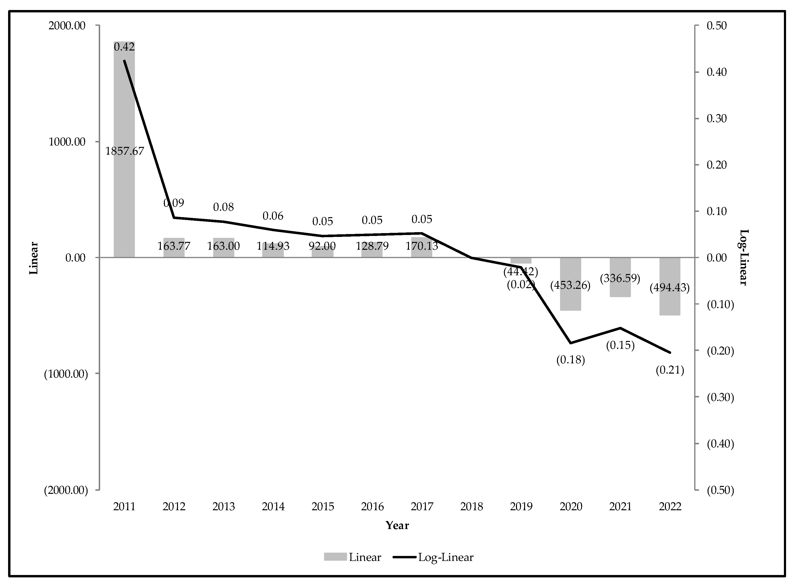
		2011	+1853.19 (32.97) ***	+1857.67 (32.97) ***
		2012	+160.93 (11.29) ***	+163.77 (11.31) ***
		2013	+160.15 (11.04) ***	+163.00 (11.06) ***
		2014	+113.14 (10.98) ***	+114.93 (11.00) ***
		2015	+89.91 (10.94) ***	+92.00 (10.96) ***
		2016	+127.49 (4.22) ***	+128.79 (4.21) ***
		2017	+169.52 (5.05) ***	+170.13 (5.04) ***
		2018	Referent	Referent
		2019	−43.88 (4.32) ***	−44.42 (4.32) ***
		2020	−471.53 (143.04) ***	−453.26 (142.16) ***
		2021	−354.02 (143.07) **	−336.59 (142.20) **
		2022	−511.07 (143.15) ***	−494.43 (142.27) ***
Census Tract (6713)
		Intercept	+3200.61 (10.85) ***	+3206.65 (10.91) ***
	Infrastructure
		EVSE 5 + Hydrogen Stations	−1.15 (0.39) ***
		EVSE		−0.26 (0.34)
		Hydrogen Stations		−10.14 (18.91)
	Race
		18 Years and Older	+0.0027 (0.0022)
		White Alone, Not Hispanic		+0.020 (0.0052) ***
		Black or African American Alone, Not Hispanic		−0.0056 (0.011)
		American Indian and Alaska Native Alone, Not Hispanic		+0.47 (0.16) ***
		Asian Alone, Not Hispanic		+0.027 (0.0043) ***
		Native Hawaiian and Other Pacific Islander Alone, Not Hispanic		−0.73 (0.14) ***
		Some Other Race Alone, Not Hispanic		−0.50 (0.22) **
		Two or More Races, Not Hispanic		−0.41 (0.066) ***
		Hispanic/Latino		+0.032 (0.0042) ***
	Sales
		ZEV 6	+0.020 (0.0015) ***
		BEV		−0.023 (0.0046) ***
		FCEV		+0.41 (0.15) ***
		PHEV		−0.017 (0.014)
	Score
		CalEnviroScreen	+7.36 (0.21) ***
		Pollution Burden		+6.47 (1.87) ***
		Population Characteristics		+47.64 (2.25) ***

¹ SE = Standard error. ² BEV = Battery electric vehicle. ³ FCEV = Fuel-cell electric vehicle. ⁴ PHEV = Plug-in hybrid electric vehicle. ⁵ EVSE = Electric Vehicle Supply Equipment. ⁶ ZEV = Zero Emission Vehicle. Includes BEVs, FCEVs, and PHEVs. *** p < 0.01. ** p < 0.05. * p < 0.10.

. The left columns of the coefficient estimates result from aggregate versions of the census-tract-level independent variables in the infrastructure category (EVSE + Hydrogen Stations); the race category (18 Years and Older); the sales category (ZEV); and the score category (CalEnviroScreen). The right columns of coefficient estimates result from disaggregate versions of the census-tract-level independent variables in the infrastructure category (EVSE and Hydrogen Stations); the race category (White Alone, Not Hispanic; Black or African American Alone, Not Hispanic; American Indian and Alaska Native Alone, Not Hispanic; Asian Alone, Not Hispanic; Native Hawaiian and Other Pacific Islander Alone, Not Hispanic; Some Other Race Alone, Not Hispanic; Two or More Races, Not Hispanic; and Hispanic/Latino); the sales category (BEV, FCEV, and PHEV); and the score category (Pollution Burden and Population Characteristics). Such results help to explore if rebates target socioeconomically vulnerable people in places where pollution is burdensome in light of infrastructural, racial, and transactional differences between census tracts from 2011 to 2022 statewide.

5.1. Diagnostics

Diagnostics for multicollinearity amongst the disaggregate versions of the census-tract-level independent variables reveal the following. Two of the eight independent variables in the race category are collinear with the Two or More Races, Not Hispanic category: the White Alone, Not Hispanic category ($\rho$ = +0.75, p = 0.00); and the Some Other Race Alone, Not Hispanic category ($\rho$ = +0.56, p = 0.00). Three of the three census-tract-level variables in the sales category are collinear: the BEV category and the FCEV category ($\rho$ = +0.76, p = 0.00); the BEV category and the PHEV category ($\rho$ = +0.90, p = 0.00); and the FCEV category and the PHEV category ($\rho$ = +0.82, p = 0.00). Nevertheless, problems with the fixed portion of the two-level model and the fixed portion of the three-level model are not evident, so the specifications are robust to multicollinearity.

5.2. Intraclass Correlation Coefficient (ICC)

The Intraclass Correlation Coefficient (ICC) measures the proportion of variance in the outcome (rebate) between groups (time and/or census tract) in random-intercept models [26]. Two methods to calculate the ICC [36] are as follows: distribute the variance to the different levels and correlate outcomes from the same group. For the first series of multilevel models, the former method to calculate the ICC distributes 2.37% of the total variance in the outcome (rebate) to the census tract level. For the second series of multilevel models, the former method to calculate the ICC distributes 3.09% of the total variance in the outcome (rebate) to the time level and 2.68% of the total variance in the outcome (rebate) to the census tract level. For the second series of multilevel models, the latter method to calculate the ICC estimates the correlation between outcomes (rebates) at the same time and in the same census tract as 5.78% [37].

5.3. Proportional Reduction of Error (PRE)

The proportional reduction of error (PRE) [38] for random-effects models is an analog to the coefficient of determination for fixed-effects models. The PRE from a full, two-level model in Table 3 to a null, two-level model is 45.53%. That is, all of the independent variables explain 45.53% of the variation in the dependent variable (Rebate) in the two-level model. The PRE from a full, three-level model in Table 4 to a null, three-level model is 52.28%. That is, all of the independent variables explain 52.28% of the variation in the dependent variable (Rebate) in the three-level model.

5.4. Two-Level Model Results

At the rebate level in the two-level model (Table 3), all of the independent variables are statistically significant at the 99% confidence level. Moreover, the signs of the statistically significant coefficient estimates are consistent with expectations. The rebates in the FCEV category are USD +2764.87 (+66.06%) higher than the rebates in the referent category (BEV). The rebates in the PHEV category are USD −1070.36 (−44.16%) lower than the rebates in the referent category (BEV).

At the census tract level in the two-level model (Table 3), the aggregate version of the race-category independent variable (18 Years and Older) is statistically significant at the 90% confidence level and the aggregate version of the score-category independent variable (CalEnviroScreen) is statistically significant at the 99% confidence level. However, the sign of the coefficient estimate for the race category is inconsistent with expectations. If the aggregate version of the race independent variable (18 Years and Older) increases by one standard deviation (1274.95), then the rebates decrease by USD −6.25. If the aggregate version of the score independent variable (CalEnviroScreen) increases by one standard deviation (15.34), then the rebates increase by USD +76.24.

At the census tract level in the two-level model (Table 3), the disaggregate versions of the race-category independent variables are statistically significant at the 90% confidence level (American Indian and Alaska Native Alone, Not Hispanic) and the 99% confidence level (White Alone, Not Hispanic; Asian Alone, Not Hispanic; Native Hawaiian and Other Pacific Islander Alone, Not Hispanic; Two or More Races, Not Hispanic; and Hispanic/Latino). The disaggregate versions of the score-category independent variable are statistically significant at the 99% confidence level (Pollution Burden and Population Characteristics). However, the signs of the coefficient estimates for the race category are inconsistent with expectations. On the one hand, if the disaggregate versions of the race independent variables White Alone, Not Hispanic; American Indian and Alaska Native Alone, Not Hispanic; Asian Alone, Not Hispanic; and Hispanic/Latino increase by one standard deviation (1001.33, 26.07, 701.01, and 971.96, respectively), then the rebates increase by USD +25.03, USD +8.08, USD +11.92, and USD +11.66, respectively. On the other hand, if the disaggregate versions of the race independent variables Native Hawaiian and Other Pacific Islander Alone, Not Hispanic; and Two or More Races Alone, Not Hispanic increase by one standard deviation (21.06 and 77.84, respectively), then the rebates decrease by USD −19.16 and USD −36.58, respectively. If the aggregate version of the score independent variable Pollution Burden increases by one standard deviation (1.50), then the rebates increase by USD +11.37. If the aggregate version of the score independent variable Population Characteristics increases by one standard deviation (1.99), then the rebates increase by USD +66.57.

5.5. Three-Level Model Results

At the rebate level in the three-level model (Table 4), all of the independent variables are statistically significant at the 99% confidence level. Moreover, the signs of the statistically significant coefficient estimates are consistent with expectations. The rebates in the FCEV category are USD +2840.46 (+69.58%) higher than the rebates in the referent category (BEV). The rebates in the PHEV category are USD −1177.61 (−51.19%) lower than the rebates in the referent category (BEV).

At the time level in the three-level model (Table 4), the 29 March 2016 dummy variable is statistically significant at the 95% confidence level and all of the year dummy variables are statistically significant at the 99% confidence level. Moreover, the signs of the statistically significant coefficient estimates are consistent with expectations. If 29 March 2016 is 1, then the rebates increase by USD +21.73 (+0.74%). The peak in rebates is in 2011 at USD +1857.67 (+42.33%) higher than in the referent year (2018), and the trough in rebates is in 2022 at USD −494.43 (−20.54%) lower than in the referent year (2018) (Figure 2).

At the census tract level in the three-level model (Table 4), the disaggregate versions of the race-category independent variables are statistically significant at the 90% confidence level (American Indian and Alaska Native Alone, Not Hispanic) and the 99% confidence level (White Alone, Not Hispanic; Asian Alone, Not Hispanic; Native Hawaiian and Other Pacific Islander Alone, Not Hispanic; Two or More Races, Not Hispanic; and Hispanic/Latino). The disaggregate versions of the sales-category independent variables (BEV and FCEV) and the score-category independent variables (Pollution Burden and Population Characteristics) are statistically significant at the 99% confidence level. However, the signs of the coefficient estimates for the race category and the sales category are inconsistent with expectations. On the one hand, if the disaggregate versions of the race independent variables White Alone, Not Hispanic; American Indian and Alaska Native Alone, Not Hispanic; Asian Alone, Not Hispanic; and Hispanic/Latino increase by one standard deviation (1001.33, 26.07, 701.01, and 971.96, respectively), then the rebates increase by USD +20.03, USD +12.25, USD +18.93, and USD +31.10, respectively. On the other hand, if the disaggregate versions of the race independent variables Native Hawaiian and Other Pacific Islander Alone, Not Hispanic; Some Other Race Alone, Not Hispanic; and Two or More Races Alone, Not Hispanic increase by one standard deviation (21.06, 12.48, and 77.84, respectively), then the rebates decrease by USD −15.37, USD −6.24, and USD −31.91, respectively. On the one hand, if the disaggregate version of the sales independent variable BEV increases by one standard deviation (907.70), then the rebates decrease by USD −20.88. On the other hand, if the disaggregate version of the sales independent variable FCEV increases by one standard deviation (19.74), then the rebates increase by USD +8.09. If the aggregate version of the score independent variable Pollution Burden increases by one standard deviation (1.50), then the rebates increase by USD +9.71. If the aggregate version of the score independent variable Population Characteristics increases by one standard deviation (1.99), then the rebates increase by USD +94.80.

6. Discussion

To return to the questions this study answers, the CVRP distributes rebates where pollution is burdensome and where people are vulnerable socioeconomically statewide. Such a result is consistent with the literature on how the CVRP distributes rebates to places where people are vulnerable to pollution [15]. Further, the statewide distribution of rebates in the CVRP is sensitive to programmatic income eligibility changes [12]. Interestingly, inconsistent with the literature on how access to infrastructure increases adoption [4], access to the infrastructure to charge and fuel BEVs, FCEVs, and PHEVs is not predictive of outcomes. Two defensible explanations for the difference in results from the present study is the disaggregation of the dependent variable and the temporal scale of the analysis. The first explanation derives from the fact that the disaggregate dependent variables in the multilevel models unmask within-census tract variation in rebates as well as between-census tract variation in rebates [13]. The temporal scale of the analysis from the calendar year of 2011 to the calendar year of 2022 also overlaps with global contraction in consumer demand due to the coronavirus (COVID-19) pandemic. The second explanation derives from the fact that the temporal scale of the analysis extends past the temporal scale (2010 to March of 2015) of Rubin and St-Louis [15]. The extension of the temporal scale past March of 2015 to include the programmatic income eligibility change on 29 March 2016 also explains the inconsistent result with regard to the race-category independent variable Hispanic/Latino. Rubin and St-Louis [15] found that the relationship between the percentage of the Hispanic or Latino population in 2010 and the number of rebates per 1000 households per census tract to be negative. However, this study found that the statewide distribution of rebates in the CVRP increases as the Hispanic/Latino population in 2020 increases (USD +31.10), regardless of the slight increase in the diversity index [39,40] from 2010 (67.7%) to 2020 (69.7%) in the State of California, whose diversity index ranks second only to the State of Hawaii from 2010 (75.1%) to 2020 (76.0%) [41]. Finally, consistent with expectations [28], this study found that the statewide distribution of rebates in the CVRP decreases as sales of BEVs increases (USD −20.88), but increases as sales of FCEVs increase (USD +8.09). Such a result suggests that the benefits from the statewide distribution of rebates in the CVRP are not specific to fuel type [9].

The contribution of this study is to explore if a statewide, AFV program distributes rebates to places where people are vulnerable socioeconomically to burdensome pollution before and after income-eligibility changes. To that end, this study extends research on consumer equity, or consumer inequity, in statewide, AFV rebate programs since the dichotomy in outcomes between people and places in national policy is not new [42], especially with regard to transportation [43,44]. Such an extension is vitally important given the results from the present study are somewhat inconsistent with the literature. Indeed, Bolton [42] highlights the balance between people prosperity versus place prosperity, a phrase from Winnick [45], to redress socioeconomic disadvantage in a national policy. Glaeser and Gottlieb [44] highlight how lower travel costs via investments in different infrastructure historically advantage places economically. Hägerstrand [43] argues “everybody has to exist spatially on an island”, but “the actual size of the island depends on the available transportation”. “During the era of more primitive transport technology, the population was nearly homogeneous with respect to daily range” [43]. However, “Improvements in transport technology have enlarged the size of the island considerably over the centuries” such that “differences between groups within the same area and differences between areas can be great” [43]. Presently, the developmental pace of more advanced transport technology is exacerbating such differences, so the efficacy of government programs to ensure a modicum of equity is important.

The logical consequence of the above argument is improvements in battery technology portending a future of greater ZEV adoption. However, Hardman and Tal [5] suggest that dissatisfaction with the convenience of the BEV and PHEV charge correlate with the discontinuance of adoption. The latter result helps us to understand why access to the infrastructure to charge and fuel BEVs, FCEVs, and PHEVs is not predictive of outcomes. The latter result also helps to provide a more accurate baseline to understand the constraints to ZEV loyalty different people in different places experience, just as Market-Majority Metrics provide a more accurate baseline to calibrate the distribution of rebates from the CVRP [9]. To that end, future research to explore the specific pollution burdens and the specific population characteristics [9,15,19] of the places where the CVRP distributes rebates statewide is important to better understand how to maximize the benefits from AFV incentives. Ongoing research to integrate individual-level socioeconomic (income) and demographic (race) information on rebate recipients, as well as qualitative components of the CVRP, into such an exploration is acknowledgement of the limitations of the present study. Research on the topics of adoption induction [21,23] and market growth [22] from AFV rebates is also ongoing and is presently in the data-collection phase.

7. Conclusions

The inclusion of spatial attributes alone in multilevel models of rebates and the inclusion of temporal attributes and spatial attributes together in multilevel models of rebates helps to control for autocorrelation in outcomes where rebates proximate in time and/or space correlate [10]. The two levels of attributes help to explore if time or space explain more of the variation in rebate outcomes. The two model specifications—a two-level model without a time level where rebates are nested within space and a three-level model with a time level where rebates are nested within time nested within space—also help to explore if the statewide distribution of rebates in the CVRP is sensitive to programmatic income eligibility changes.

Taken together, outcomes proximate in time and space correlate modestly. The correlation between rebates at the same time and in the same census tract (5.78%) is slight but consistent with the literature on how adopters cluster in space [10,46]. Time explains slightly more of the variation in rebate outcomes than space given that the three-level model distributes slightly more of the variation in rebate outcomes to the time level than the census tract level (3.09% vs. 2.68%). Such a result validates the inclusion of time and space at different levels of analysis [37]. Further, the PRE for the two-level model (45.53%), as well as the PRE for the three-level model (52.28%), attest to the value of the model specifications without time and with time. To be clear, the latter model specifications nest time within census tracts, rather than nesting census tracts within time, because of the sample size requirements for the accurate estimation of the standard errors of the variances at the group level in a multilevel model [47].

References

- 2023 Light-Duty Vehicle Registration Counts by State and Fuel Type. Available online: https://afdc.energy.gov/vehicle-registration (accessed on 28 May 2025).
- Electric Vehicle Registrations by States. Available online: https://afdc.energy.gov/data/10962 (accessed on 28 May 2025).
- Krupa, J.; Rizzo, D.; Eppstein, M.; Lanute, D.; Gaalema, D.; Lakkaraju, K.; Warrender, C. Analysis of a Consumer Survey on Plug-In Hybrid Electric Vehicles. Transp. Res. A-Pol. 2014, 64, 1431. [Google Scholar] [CrossRef]
- Narassimhan, E.; Johnson, C. The Role of Demand-Side Incentives and Charging Infrastructure on Plug-In Electric Vehicle Adoption: Analysis of US States. Environ. Res. Lett. 2018, 13, 074032. [Google Scholar] [CrossRef]
- Hardman, S.; Tal, G. Understanding Discontinuance Among California’s Electric Vehicle Owners. Nature Energy 2021, 6, 538–545. [Google Scholar] [CrossRef]
- Adepetu, A.; Keshav, S. The Relative Importance of Price and Driving Range of Electric Vehicle Adoption: Los Angeles Case Study. Transportation 2017, 44, 35373. [Google Scholar] [CrossRef]
- Sheldon, T.; Dua, R.; Abdullah Alharbi, O. Electric Vehicle Subsidies: Time to Accelerate or Pump the Brakes? Energ. Econ. 2023, 120, 106641. [Google Scholar] [CrossRef]
- Borenstein, S.; Davis, L. The Distributional Effects of US Clean Energy Tax Credits. Tax Pol. Econ. 2016, 30, 191–234. [Google Scholar] [CrossRef]
- Williams, B. Assessing Progress and Equity in the Distribution of Electric Vehicle Rebates Using Appropriate Comparisons. Transp. Policy 2023, 137, 141–151. [Google Scholar] [CrossRef]
- Guo, S.; Kontou, E. Disparities and Equity Issues in Electric Vehicles Rebate Allocation. Energ. Policy 2021, 154, 112291. [Google Scholar] [CrossRef]
- Rebate Statistics. Available online: https://cleanvehiclerebate.org/rebate-statistics (accessed on 28 May 2025).
- DeShazo, J.; Sheldon, T.; Carson, R. Designing Policy Incentives for Cleaner Technologies: Lessons from California’s Plug-In Electric Vehicle Rebate Program. J. Environ. Econ. Manag. 2017, 84, 18–43. [Google Scholar] [CrossRef]
- Khattak, Z.; Khattak, A. Spatial and Unobserved Heterogeneity in Consumer Preferences for Adoption of Electric and Hybrid Vehicles: A Bayesian Hierarchical Modeling Approach. Int. J. Sustain. Transp. 2023, 17, 1–14. [Google Scholar] [CrossRef]
- AB 32 Global Warming Solutions Act of 2006. Available online: https://ww2.arb.ca.gov/resources/fact-sheets/ab-32-global-warming-solutions-act-2006 (accessed on 28 May 2025).
- Rubin, D.; St-Louis, E. Evaluating the Economic and Social Implications of Participation in Clean Vehicle Rebate Programs: Who’s In, Who’s Out? Transp. Res. Record 2016, 2598, 67–74. [Google Scholar] [CrossRef]
- Johnson, C.; Williams, B. Characterizing Plug-In Hybrid Electric Vehicle Consumers Most Influenced by California’s Electric Vehicle Rebate. Transp. Res. Record 2017, 2628, 23–31. [Google Scholar] [CrossRef]
- Canepa, K.; Hardman, S.; Tal, G. An Early Look at Plug-In Electric Vehicle Adoption in Disadvantaged Communities in California. Transp. Policy 2019, 78, 19–30. [Google Scholar] [CrossRef]
- Lee, J.; Hardman, S.; Tal, G. Who is Buying Electric Vehicles in California? Characterising Early Adopter Heterogeneity and Forecasting Market Diffusion. Energy Res. Soc. Sci. 2019, 55, 218–226. [Google Scholar] [CrossRef]
- Ju, Y.; Cushing, L.; Morello-Frosch, R. An Equity Analysis of Clean Vehicle Rebate Programs in California. Clim. Change 2020, 162, 2087–2105. [Google Scholar] [CrossRef]
- Pallonetti, N.; Williams, B. Refining estimates of fuel-cycle greenhouse-gas emission reductions associated with California’s clean vehicle rebate project with program data and other case-specific inputs. Energies 2021, 14, 4640. [Google Scholar] [CrossRef]
- Williams, B.; Anderson, J. Strategically Targeting Plug-In Electric Vehicle Rebates and Outreach Using “EV Convert” Characteristics. Energies 2021, 14, 1899. [Google Scholar] [CrossRef]
- Lee, J.; Cho, M.; Tal, G.; Hardman, S. Do Plug-In Hybrid Adopters Switch to Battery Electric Vehicles (And Vice Versa)? Transport. Res. D-Transp. Environ. 2023, 119, 103752. [Google Scholar] [CrossRef]
- Williams, B.; Anderson, J. From Low Initial Interest to Electric Vehicle Adoption: “EV Converts” in New York State’s Rebate Program. Transp. Res. Record 2023, 2677, 866–882. [Google Scholar] [CrossRef]
- Faust, J.; August, L.; Bangia, K.; Galaviz, V.; Lechty, J.; Prasad, S.; Schmitz, R.; Slocombe, A.; Welling, R.; Wieland, W.; et al. CalEnvironScreen 3.0. Available online: https://oehha.ca.gov/media/downloads/calenviroscreen/report/ces3report.pdf (accessed on 28 May 2025).
- Jones, K.; Bullen, N. Contextual Models of Urban House Prices: A Comparison of Fixed-and Random-Coefficient Models Developed by Expansion. Econ. Geogr. 1994, 70, 252–272. [Google Scholar] [CrossRef]
- Raudenbush, S.; Bryk, A. Hierarchical Linear Models: Applications and Data Analysis, 2nd ed.; Sage: Thousand Oaks, CA, USA, 2002; ISBN 978-0-76191-904-9. [Google Scholar]
- California Consumer Price Index (1995–2023). Available online: https://www.cdfa.ca.gov/AHFSS/cabb/docs/202406_notice_Feb_California_Consumer_Price_Index_1955-2024.pdf (accessed on 28 May 2025).
- 2022 Incremental Purchase Cost Methodology and Results for Clean Vehicles. Available online: https://www.energy.gov/sites/default/files/2022-12/2022.12.23%202022%20Incremental%20Purchase%20Cost%20Methodology%20and%20Results%20for%20Clean%20Vehicles.pdf (accessed on 28 May 2025).
- Implementation Manual for the Clean Vehicle Rebate Project (CVRP). Available online: https://cleanvehiclerebate.org/sites/default/files/docs/nav/transportation/cvrp/documents/CVRP-Implementation-Manual.pdf (accessed on 28 May 2025).
- Alternative Fueling Station Locator. Available online: https://afdc.energy.gov/stations/#/analyze?country=US&access=public&access=private&status=E&status=P&status=T (accessed on 28 May 2025).
- Population 18 Years and Older by Race (Not Hispanic/Latino) and Hispanic/Latino: 2020 Census. Available online: https://dof.ca.gov/wp-content/uploads/sites/352/Forecasting/Demographics/Documents/2020Census_CT2_Race-HispExcl_RedistrictingFile.xlsx (accessed on 28 May 2025).
- ZEV and Infrastructure Stats Data. Available online: https://www.energy.ca.gov/files/zev-and-infrastructure-stats-data (accessed on 28 May 2025).
- Faust, J.; August, L.; Alexeef, G.; Bangia, K.; Cendak, R.; Cheung-Sutton, E.; Cushing, L.; Galaviz, V.; Kakir, T.; Lechty, J.; et al. California Communities Environmental Health Screening Tool, Version 2.0 (CalEnvironScreen 2.0). Available online: https://oehha.ca.gov/media/CES20FinalReportUpdateOct2014.pdf (accessed on 28 May 2025).
- August, L.; Bangia, K.; Plummer, L.; Prasad, S.; Ranjbar, K.; Slocombe, A.; Wieland, W. CalEnvironScreen 4.0. Available online: https://oehha.ca.gov/calenviroscreen/report/calenviroscreen-40 (accessed on 28 May 2025).
- About CalEnviroScreen. Available online: https://oehha.ca.gov/calenviroscreen/about-calenviroscreen (accessed on 28 May 2025).
- Hox, J.; Moerbeek, M.; van de Schoot, R. Multilevel Analysis: Techniques and Applications, 3rd ed.; Routledge: New York, NY, USA, 2018; ISBN 978-1-138-12140-9. [Google Scholar]
- Tranmer, M.; Steel, D. Ignoring a Level in a Multilevel Analysis: Evidence from UK Census Data. Environ. Plann. A 2001, 33, 941–948. [Google Scholar] [CrossRef]
- Snijders, T.; Bosker, R. Multilevel Analysis: An Introduction to Basic and Advanced Multilevel Modelling, 2nd ed.; Sage: Los Angeles, CA, USA, 2012; ISBN 978-1-84920-200-8. [Google Scholar]
- Blau, P. Inequality and Heterogeneity: A Primitive Theory of Social Structure, 1st ed.; Free Press: New York, NY, USA, 1977; ISBN 978-0-02903-660-0. [Google Scholar]
- California: 2020 Census. Available online: https://www.census.gov/library/stories/state-by-state/california-population-change-between-census-decade.html (accessed on 28 May 2025).
- Meyer, P.; McIntosh, S. The USA Today Index of Ethnic Diversity. Int. J. Public Opin. R. 1992, 4, 51–58. [Google Scholar] [CrossRef]
- Bolton, R. ‘Place Prosperity vs People Prosperity’ Revisited: An Old Issue with a New Angle. Urban Stud. 1992, 29, 185–203. [Google Scholar] [CrossRef]
- Hägerstrand, T. What About People in Regional Science? Pap. Reg. Sci. Assoc. 1970, 24, 7–21. [Google Scholar] [CrossRef]
- Glaeser, E.; Gottlieb, J. The Economics of Place-Making Policies. Brook. Pap. Econ. Act. 2008, 2008, 155–239. [Google Scholar] [CrossRef]
- Winnick, L. Place Prosperity vs People Prosperity: Welfare Considerations in the Geographic Distribution of Economic Activity. In Essays in Urban Land Economics; Grebler, L., Ed.; Real Estate Research Program: Los Angeles, CA, USA, 1966; pp. 273–283. [Google Scholar]
- Liu, X.; Roberts, M.; Sioshansi, R. Spatial Effects on Hybrid Electric Vehicle Adoption. Transport. Res. D-Transp. Environ. 2017, 52, 85–97. [Google Scholar] [CrossRef]
- Maas, C.; Hox, J. Sufficient Sample Sizes for Multilevel Modeling. Methodol. Eur. J. Res. Methods Behav. Soc. Sci. 2005, 1, 86–92. [Google Scholar]