Quantum-Inspired Spatio-Temporal Inference Network for Sustainable Car-Sharing Demand Prediction

Abstract

Accurate car-sharing demand prediction is a key factor in enhancing the operational efficiency of shared mobility systems. However, mobility data often exhibit temporal, spatial, and spatio-temporal interdependencies that pose significant challenges for conventional models. These models typically struggle to capture nonlinear and high-dimensional patterns. Existing methods struggle to model entangled relationships across these modalities and lack scalability in dynamic urban environments. This paper presents the Quantum-Inspired Spatio-Temporal Inference Network (QSTIN), an enhanced approach that builds upon our previously proposed Explainable Spatio-Temporal Inference Network (eX-STIN). QSTIN integrates a Quantum-Inspired Neural Network (QINN) into the fusion module, generating complex-valued feature representations. This enables the model to capture intricate, nonlinear dependencies across heterogeneous mobility features. Additionally, Quantum Particle Swarm Optimization (QPSO) is applied at the final prediction stage to optimize output parameters and improve convergence stability. Experimental results indicate that QSTIN consistently outperforms both conventional baseline models and the earlier eX-STIN in predictive accuracy. By enhancing demand prediction, QSTIN supports efficient vehicle allocation and planning, reducing energy use and emissions and promoting sustainable urban mobility from both environmental and economic perspectives.

1. Introduction

Sustainable urban development relies increasingly on the evolution of mobility systems to meet the environmental and economic demands of growing cities. Shared mobility services, such as car-sharing, have emerged as effective alternatives to private vehicle ownership. These services help reduce emissions, ease traffic congestion, and enhance the overall efficiency of urban transportation. These systems contribute to sustainability by promoting energy-efficient travel, reducing greenhouse gas emissions, and maximizing infrastructure utilization. Alongside these environmental benefits, they also offer economic advantages, such as lower operational costs, improved fleet efficiency, and more adaptive transport planning. The effectiveness of such systems depends heavily on accurate demand predictions, which are essential for efficient resource allocation and timely service responsiveness. However, accurately predicting the car-sharing demand remains a significant challenge because of the complex and interdependent nature of urban mobility data. These dependencies are characterized by temporal sequences, spatial distributions, and spatio-temporal dynamics. Effectively capturing these complexities is crucial for developing predictive frameworks that can adapt to evolving mobility patterns and support long-term sustainability.

Although various machine and deep learning methods have been widely applied to this task, two persistent limitations remain. First, many models process mobility features independently, preventing them from capturing the joint structures that arise when the temporal and spatial dynamics interact. Second, traditional architecture often fall short of modeling the nonlinear, high-dimensional, and nonstationary nature of real-world transportation systems, limiting their predictive accuracy and adaptability in complex environments [1]. Addressing these challenges requires a more advanced modeling approach that can capture deeply entangled higher-order dependencies across multimodal inputs, while maintaining scalability in real-world deployments.

To overcome these limitations, we propose a quantum-inspired spatio-temporal inference network (QSTIN), an advanced framework that extends our previously developed explainable spatio-temporal inference network (eX-STIN) [2]. Although eX-STIN leverages a modular structure combining temporal, spatial, and spatio-temporal units with feature reduction and explainable AI techniques to improve accuracy and interpretability, it remains limited in representing nonlinear feature interactions in high-dimensional data. To fill these gaps, QSTIN introduces two core methodological advancements. First, it incorporates a quantum-inspired neural network (QINN) into the fusion module, enabling the transformation of inputs into complex-valued representations that better capture nonlinear dependencies across mobility features [3,4]. Second, quantum particle swarm optimization (QPSO) is applied to the final regression stage to conduct global hyperparameter optimization. By leveraging quantum search dynamics, QPSO improves convergence stability and enhances adaptability under the nonstationary and dynamic conditions typical of urban mobility systems [5,6].

The contributions of this work are threefold, as follows: (i) the integration of a quantum-inspired fusion module based on complex-valued neural representations to capture complex, nonlinear interdependencies across temporal, spatial, and spatio-temporal features; (ii) the application of QPSO to the final regression layer to improve convergence and achieve global optimization of prediction outputs; and (iii) the comprehensive benchmarking of QSTIN against conventional machine learning models, advanced spatio-temporal architectures, and its predecessors to validate the effectiveness of the proposed enhancements.

The remainder of this paper is organized as follows. Section 2 reviews related work on predictive modeling approaches and quantum-inspired methods relevant to transportation demand prediction. Section 3 describes the proposed methodology in detail. Section 4 describes the experimental framework used to evaluate the performance of the proposed model. Section 5 analyzes the results and discusses the key findings. Finally, Section 6 concludes the paper and outlines potential directions for future research.

2. Literature Review

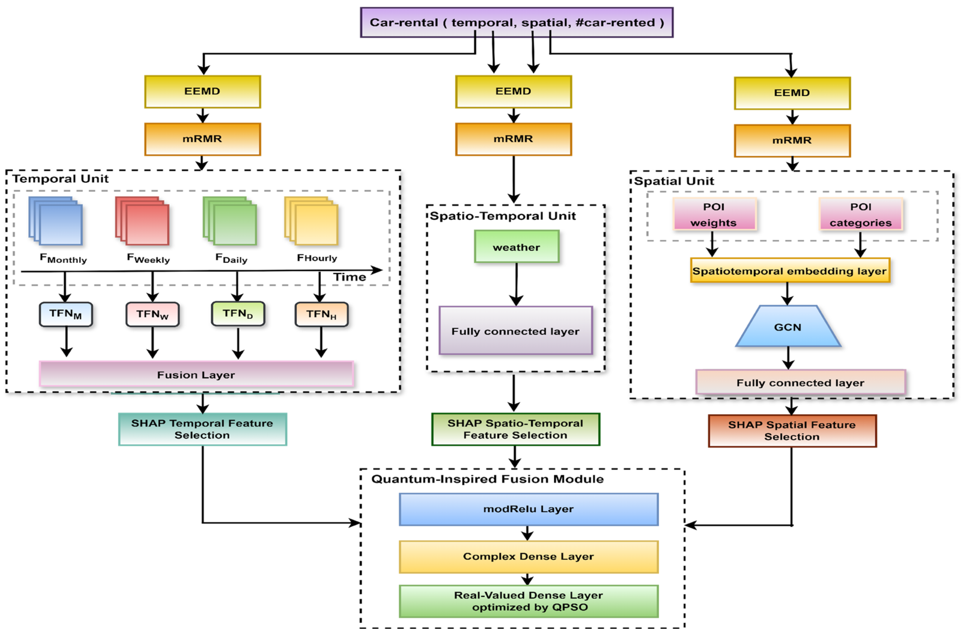
As urban populations continue to expand, car-sharing systems have become increasingly vital in reducing congestion, emissions, and environmental impact by promoting shared vehicular access [7]. Accurate demand prediction is essential for minimizing operational inefficiencies and ensuring effective vehicle allocation [8]. However, despite ongoing progress, existing models often struggle to capture complex relationships among temporal, spatial, and spatio-temporal mobility factors in urban datasets, leading to limited prediction accuracy. Prior studies have emphasized these limitations. For instance, Chen et al. [9] and Chai et al. [10] examined multivehicle optimization frameworks incorporating drones, while Luan [11] proposed hybrid logistics solutions combining aerial and ground transportation. These studies underscore the importance of precise modeling in urban mobility and logistics systems. Petri et al. [12] and Hsieh et al. [13] further demonstrated how the absence of fine-grained temporal detail and incomplete feature integration can result in resource underutilization or oversupply. Feng et al. [14] highlighted the need for modeling both zone-based and origin–destination (OD) demands using a multitask matrix factorized graph neural network, showing that traditional single-task frameworks often fail to account for dual-layered urban demand structures effectively.

Recent research has increasingly turned to advanced deep learning models to address the challenges of limited prediction accuracy. Approaches such as graph convolutional networks (GCNs), gated recurrent units (GRUs), and hybrid architectures have shown promise in capturing spatial and temporal dependencies more effectively. Wang and Deng [15] demonstrated the ability of GCNs to extract spatially structured patterns, while GRUs have shown effectiveness in modeling temporal dependencies. He et al. [16] combined spatial and temporal reasoning for traffic flow prediction using hybrid deep learning techniques, and Yuan et al. [17] incorporated contextual inputs, such as weather and time, to improve forecasting accuracy. Despite these advances, many of these approaches fail to generalize across complex, multimodal urban environments due to the limited integration of heterogeneous data and reliance on heuristic optimization. Architectures like ST-MetaNet [18] and 3D-TGCN [19] introduced attention and gating mechanisms to improve temporal–spatial modeling but continue to face issues, such as overfitting and limited scalability on large datasets. Building on these advances, Ou et al. [20] proposed STP-TrellisNets+, a spatial–temporal parallel framework integrating TrellisNet-based encoder–decoder structures with dynamic graph convolutional modules, demonstrating improved multistep forecasting accuracy for metro station flows by modeling both short- and long-term dependencies. This line of research illustrates the potential of integrating modular spatial and temporal learning components in transport prediction systems.

However, despite the progress achieved with advanced deep learning architectures, challenges, such as scalability, the integration of heterogeneous data, and capturing complex feature interactions, remain. Quantum-inspired methods have emerged as promising alternatives for enhancing representation learning and optimization in complex prediction tasks. Originating from the physical sciences, these methods provide enhanced computational capacity through complex-valued modeling and probabilistic search dynamics. Kardashin et al. [21] demonstrated the potential of quantum circuits for the precise computation of observables, while Huerga et al. [22] applied quantum kernels and support vector machines to predict human behavior. Similarly, Surendiran et al. [23] found that quantum machine learning significantly outperformed classical methods in weather forecasting. Within the transportation domain, Li et al. [24] and Zhuang et al. [25] revealed the effectiveness of quantum algorithms for solving routing and congestion problems under computational constraints. Qu et al. [26] proposed a temporal–spatial quantum GCN, which achieved improved robustness and lower error rates in congestion forecasting.

Recent studies have introduced quantum-inspired neural networks (QINNs) to enhance spatio-temporal inference and complex pattern recognition. QINNs leverage complex-valued representations that encode both phase and amplitude information, enabling the modeling of higher-order interdependencies in multimodal data [27,28]. Tomal et al. [29] demonstrated that QINNs outperform conventional networks in non-stationary time-series classification, while Thakkar et al. [30] reported similar benefits in financial forecasting tasks, attributing their success to phase-aware feature encoding. To further optimize learning, quantum particle swarm optimization (QPSO) has been applied to global hyperparameter tuning. QPSO merges quantum probability characteristics with swarm intelligence to improve exploration of the parameter space and reduce susceptibility to local optima [31]. Unlike traditional gradient-based optimization, QPSO supports adaptive learning in non-convex and noisy environments. Its effectiveness has been confirmed across multiple domains. Alvarez-Alvarado et al. [32] introduced bounded potential field-based QPSO for enhanced performance on standard benchmarks, while Fallahi and Taghadosi [33] developed a soliton-inspired variant with improved convergence speed. In transportation modeling, Li et al. [34] used QPSO for traffic prediction with notable gains in accuracy, and Sengupta et al. [35] integrated QPSO with fuzzy clustering to enhance uncertainty modeling.

The integration of QINN and QPSO into spatio-temporal inference frameworks directly addresses the following two core gaps in prior research: the inability to capture complex feature relationships and the lack of scalable, generalizable learning under dynamic urban conditions. Building on our earlier eX-STIN model, which introduced modular inference units and interpretability through SHAP and feature reduction, the proposed QSTIN architecture incorporates quantum-inspired mechanisms within a unified learning framework. Specifically, QINN enables complex-valued fusion for modeling higher-order feature interactions, while QPSO provides efficient global optimization to improve convergence and adaptability. Together, these enhancements advance the generalization capacity of predictive models in high-dimensional, evolving urban datasets.

3. Methodology

This section presents the quantum-inspired spatio-temporal inference network (QSTIN) for car-sharing demand prediction, building on the eX-STIN architecture. Conventional models often fail to capture complex temporal, spatial, and spatio-temporal dependencies and rely on heuristic optimization, limiting their generalizability. QSTIN addresses these issues by integrating QINN for complex-valued feature fusion and QPSO for effective, global optimization in the regression layer.

QSTIN retains eX-STIN’s use of ensemble empirical mode decomposition (EEMD) for multiscale feature extraction and minimum redundancy maximum relevance (mRMR) for feature selection, while maintaining SHAP-based interpretability after each unit. The fusion module incorporates QINN to better capture entangled relationships, and QPSO is used at the output to fine-tune prediction parameters for improved adaptability and accuracy.

As shown in Figure 1, QSTIN comprises the following four stages: (i) feature extraction and selection, (ii) spatio-temporal inference modules, (iii) SHAP-based interpretability with complex-valued fusion, and (iv) QPSO-optimized regression output. These components enable reliable, interpretable, and accurate demand prediction in complex urban settings.

The QSTIN model includes the following three categories of input features: temporal features ($G_t$), representing demand variation over time; spatial features ($G_{POI}$), capturing the influence of surrounding points of interest near car-sharing stations; and spatio-temporal features ($G_{me}$) that reflect weather conditions distributed across both spatial and temporal dimensions.

3.1. Feature Extraction

Urban mobility often exhibits high nonlinearity and non-stationarity. To address this, we employ EEMD as a preprocessing step for all feature types [36]. EEMD decomposes the original signals into a finite number of intrinsic mode functions (IMFs) and a residual component, enabling the model to isolate multiscale information and reduce non-stationarity [37]. This process is uniformly applied to the temporal, spatial, and spatio-temporal input features, as defined by the following generalized formulation:

$$G_m^{IMF}=\sum _{k=1}^K\left(\sum _{i=1}^N{C}_{i,k}\left(G_m\right)\right)+R\left(G_m\right),\hspace{1em}m\in \left\{t,poi,me\right\}$$

(1)

where:

$G_m^{IMF}$: reconstructed signal from the IMFs and residual for modality $m$, where $m\in \left\{t,poi,me\right\}$, representing temporal, spatial, and spatio-temporal features.

$G_m$: the signal for modality $m$.

$C_{i,k}\left(G_m\right)$: IMFs from temporal data, with $i$ as the IMF index and $k$ as the trial index.

$R\left(G_m\right)$: residual pattern after decomposing $G_m$.

3.2. Feature Selection

To retain only the most relevant and non-redundant features from the decomposed signals, we employ the mRMR algorithm. The mRMR approach identifies the most informative features by maximizing their relevance to the target variable, while minimizing redundancy among the selected features [38]. This is achieved through the computation of mutual information, which quantifies both the relevance $I\left(F_i^m;Y\right)$ between each feature $F_i^m$ and the output $Y$ and the redundancy $I\left(F_i^m;F_j^m\right)$ between pairs of features. Formally, the selection criterion applied to the IMF components derived from each modality $G_m$ (where $m\in \left\{t,poi,me\right\}$) is defined as follows:

$$mRMR\left(G_m^{IMF}\right)={\displaystyle \frac{1}{\left|S_m\right|}}\sum _{iϵS}I\left(F_i^m;Y\right)-{\displaystyle \frac{1}{{\left|S_m\right|}^2}}\sum _{i,jϵS}I\left(F_i^m;F_j^m\right),\hspace{1em}m\in \left\{t,poi,me\right\}$$

(2)

where:

$S_m$: subset of selected features from $G_m^{IMF}$.

$F_i^m$: $i\mathrm{t}\mathrm{h}$ features within the subset $S_m$.

$I\left(F_i^m;F_j^m\right)$: mutual information between features $F_i^m$ and $F_j^m$.

$I\left(F_i^m;Y\right)$: mutual information between features $F_i^m$ and the target variable $Y$.

This process ensures that the retained features are both relevant and non-redundant, improving the efficiency and predictive performance of the model.

3.3. Predictive Model

This section discusses the prediction model, which is an extension of our eX-STIN model [2]. The predictive model comprises the following three units: a temporal feature unit, a spatial feature unit, and a spatio-temporal feature unit. SHAP-based interpretability follows each unit to quantify the feature impact before fusion.

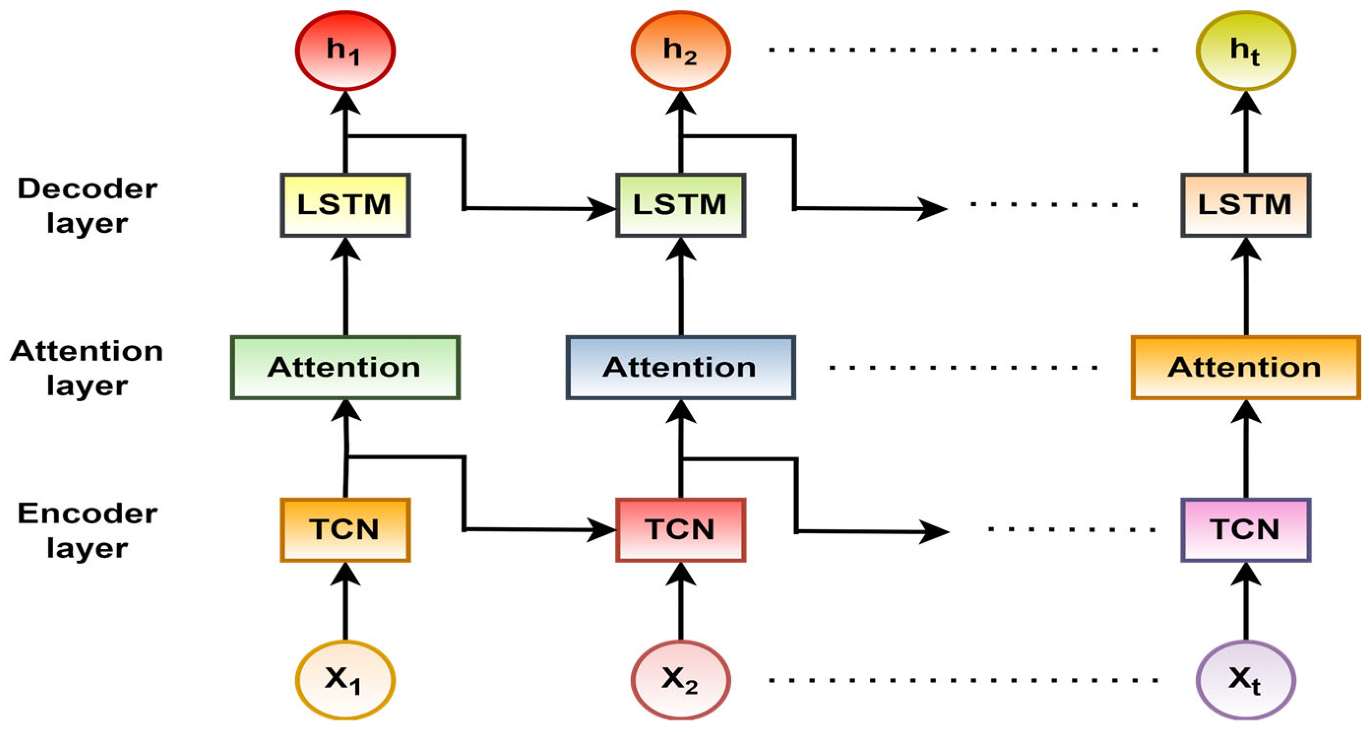
3.3.1. Temporal Feature Unit

Temporal features are retrieved at hourly, daily, weekly, and monthly intervals. Each layer has a temporal fusion network (TFN) architecture [2], which efficiently captures temporal correlations, as depicted in Figure 2.

1.

Encoder: temporal convolutional network (TCN)

TCN functions as an encoder by analyzing selected temporal data and is optimized for the efficient capture of long-term dependencies.

$$G_t^{TCN}=ReLU\left(W_t\odot F_t+b_t\right)$$

(3)

where:

$G_t^{TCN}$: output of the TCN.

$W_t$: weight matrix of the convolutional filter.

$b_t$: bias term.

$\odot$: convolution operation.

Following encoding, the output is batch-normalized to enhance training stability and facilitate faster convergence before being processed by the attention mechanism.

$$G_t=\gamma \left({\displaystyle \frac{G_t^{TCN}-{\mu }_B}{\sqrt{\left({\sigma }_B^2+\epsilon \right)}}}\right)+\beta$$

(4)

where:

$G_t$: batch-normalized output at a specific time step $t$.

${\mu }_B,{\sigma }_B^2$: mean and variance computed over the batch.

$\gamma ,\beta$: learnable parameters specific to each feature dimension.

$\epsilon$: small constant added for numerical stability.

2.

Attention mechanism layer

The attention mechanism enables the model to weigh contributions from various sequences at each time step, thereby improving the prediction of current values in time series analysis. By employing LSTM as the decoder, the model extracts the hidden state $H_i$ at each time step $i$, which is then compared with the encoder’s hidden representation ${\widehat{G}}_t$ at each corresponding time step $t$. This comparison supports precise temporal alignment and comprehensive context integration.

$$e_{it}=a\left(H_i{G}_t\right)$$

(5)

$$a_{it}={\displaystyle \frac{exp\left(e_{it}\right)}{{\sum }_{k=1}^{T}exp\left(e_{ik}\right)}}$$

(6)

$${\widehat{G}}_i=\sum _{j=1}^T\left(a_{ij}{G}_t\right)$$

(7)

where:

$e_{it}$: number of attentional correlations from the moment $t$ to moment $i$.

$a_{it}$: attentional weight.

$i$: current time step in the decoder.

$t$: time steps in the encoder’s output.

$T$: number of time steps in the encoder output.

$k$: iterator in the normalization sum.

3.

Decoder: long short-term memory layer (LSTM)

By incorporating contextual information from the attention mechanism, the LSTM decoder generates more accurate sequences. It operates through the input ($i_i$), forget ($f_i$), and output ($o_i$) gates. The context vector ${\widehat{G}}_i$ generated by the attention mechanism is incorporated into the subsequent decoding layer as part of the input, facilitating the computation of the output $y_j$:

$$i_i=\sigma (W_i.\left[H_{i-1}{y}_{i-1}{\widehat{G}}_i\right]+b_i)$$

(8)

$$f_i=\sigma (W_f.\left[H_{i-1}{y}_{i-1}{\widehat{G}}_i\right]+b_f)$$

(9)

$$o_i=\sigma (W_o.\left[H_{i-1}{y}_{i-1}{\widehat{G}}_i\right]+b_o)$$

(10)

$$g_i=tanh(W_g\left[H_{i-1}{y}_{i-1}{\widehat{G}}_i\right]+b_g)$$

(11)

$$c_i=i_i\odot g_i+f_i\odot c_{i-1}$$

(12)

$$H_i=o_i\odot tanh\left(c_i\right)$$

(13)

where:

$W_i, W_f, W_o, W_g$: weight matrices for input gate, forget gate, output gate, and candidate cell state, respectively.

$b_i,$ $b_f, b_o,b_g:$ bias terms for the input gate, forget gate, output gate, and candidate cell state, respectively.

$c_i$: current cell state.

$c_{i-1}$: cell state from the previous time step.

$H_i$: current hidden state.

$\sigma$: sigmoid activation function.

$\odot$: element-wise multiplication.

To efficiently integrate the outcomes from the decoders that work at various temporal scales, we employ a fully connected layer. This approach enhances the model’s ability to identify complex interdependencies within the data.

$$X_{sp}=ReLU(W_{sp}.\left[H_p+H_D+H_W+H_M\right]+b_{sp}$$

(14)

where:

$H_p,H_D, H_W,H_M$: represents the concatenated outputs from the LSTM decoders at four different time scales (daily, weekly, monthly, and yearly).

$W_{sp}$: weight matrix of the fully connected layer.

$b_{sp}$: bias of the dense fully connected layer.

3.3.2. Spatial Feature Unit

A dedicated spatial feature unit is implemented to effectively process POI-related information. This architecture comprises the following components:

1.

Spatial density calculation

The density of POIs around each car-sharing station is calculated to assess the geographical characteristics of urban areas. This metric indicates the local activity level and service availability, which are important determinants of mobility demand. The density computation considers the quantity of adjacent POIs and their spatial closeness to the station, within a specified threshold radius $R$.

The distance between a station $S_i$ and a ${POI}_j$ is calculated using the Haversine formula, which computes the great-circle distance between two geographic coordinates based on their latitude and longitude [2]. This distance is denoted as $d\left(S_i,{POI}_j\right)$, representing the spherical distance between the coordinates of the station $S_i$ and ${POI}_{j }$.

The POI density indicator $D_{{POI}_j}$ is then formulated as:

$$D_{{POI}_j}=\left\{\begin{array}{c}1 if d\left(S_i,{POI}_j\right) \le 1 \\ 0 otherwise\end{array}\right.$$

(15)

2.

Regression model

Car-sharing demand exhibits overdispersion, where the variance significantly exceeds the mean. To address this statistical property, a negative binomial regression model is employed for parameter estimation, which is more appropriate than a Poisson model under such conditions [39].

The model estimates the number of rentals $\left(u_i\right)$ at a station $i$ as a function of POI category densities. It includes an intercept term (${\beta }_0)$, regression coefficients $({\beta }_1,\dots ,{\beta }_n)$ corresponding to each POI feature $(x_1,\dots ,x_n)$, and an error term ($\epsilon$). These POI features reflect various urban functionalities near each station.

The regression formulation is given as follows:

$$ln\left(u_i\right)={\beta }_0+{\beta }_1·x_1+{\beta }_2·x_2+\dots +{\beta }_n·x_n+\epsilon$$

(16)

The parameters are estimated using maximum likelihood estimation (MLE), maintaining a $5\%$ significance level. This model enables the identification of statistically significant POI categories influencing demand, thereby supporting feature selection and model interpretability.

3.

Spatiotemporal embedding layer

The selected POI features $F_{POI}$, together with the corresponding weight vector $W_{POI}$, which includes the regression coefficients obtained from Equation (16), are provided as input to a spatiotemporal embedding layer, as follows:

$$E_{POI}=ReLU\left(W_{POI}.F_{POI}\right)$$

(17)

4.

Graph convolutional network layer (GCN)

The output generated by the spatiotemporal embedding layer is forwarded to a GCN, where a mean aggregation function is implemented to effectively capture spatial dependencies among POIs:

$$H_{POI}^n=\left({\displaystyle \frac{1}{D_{POI}}}\right)AGG{.E}_{POI}.A_{POI}$$

(18)

5.

Fully connected layer

The unit employs a fully connected layer to enhance the model’s accurate demand predictions, as follows:

$$X_{MC}=ReLU(W_{MC}.H_{POI}^n+b_{MC})$$

(19)

where:

$W_{MC}$: weight of the fully connected layer.

$b_{MC}$: bias of the fully connected layer.

3.3.3. Spatio-Temporal Feature Unit

The selected meteorological features $F_{ME}$ are input into a fully connected neural network to effectively model the influence of weather conditions over temporal and spatial dimensions.

$$X_{ME}=ReLU(W_{ME}.F_{ME}+b_{ME})$$

(20)

where:

$W_{ME}$: weight of the fully connected layer.

$b_{ME}$: bias of the fully connected layer.

3.3.4. Quantum Inspired Fusion Module

To maintain interpretability, we employ SHAP (Shapley additive explanations) to quantify feature importance across temporal, spatial, and spatio-temporal units [40]. As a model-agnostic method, SHAP provides consistent, localized insights into each feature’s contribution to predictions [41], which is essential in multimodal architectures with heterogeneous inputs [42]. The SHAP-derived outputs $X_{sp}^{SHAP}$, $X_{MC}^{SHAP}$, and $X_{ME}^{SHAP}$ are normalized before fusion to ensure scale alignment and preserve interpretability throughout the inference pipeline.

The concatenated normalized SHAP outputs provide a comprehensive representation, enabling QINN to jointly process multimodal data and effectively model entangled dependencies across temporal, spatial, and spatio-temporal domains:

$$X_{concat}=(X_{sp}^{SHAP},X_{MC}^{SHAP},X_{ME}^{SHAP})$$

(21)

where:

$X_{sp}^{SHAP}$: normalized SHAP output from the temporal feature unit.

$X_{Mc}^{SHAP}$: normalized SHAP output from the spatial feature unit.

$X_{ME}^{SHAP}$: normalized SHAP output from the spatio-temporal feature unit.

This SHAP-based fusion approach not only preserves the interpretability of each unit but also enhances the transparency and reliability of the quantum-inspired prediction.

1.

Encoding multimodal features in the complex domain

To enable quantum-inspired processing within the QINN framework, the concatenated real-valued feature vector is transformed into a complex-valued representation. This transformation allows the network to simulate quantum-like interactions and enhances its ability to capture intricate dependencies across input modalities [43]. The resulting complex-valued representation $X_i$ serves as the input to QINN. By operating in the complex domain, QINN is equipped to model higher-order interactions that are typically unrepresentable in real-valued spaces, thereby enhancing the fusion process and improving feature expressiveness across spatial, temporal, and spatio-temporal modalities [44].

$$X_i=X_{concat}^{real}+i.X_{concat}^{image}$$

(22)

where:

$X_{concat}^{real}$: original real-valued concatenated features.

$i$: imaginary component generated through a learned transformation.

$X_{concat}^{image}$: imaginary unit.

2.

Nonlinear activation in the complex domain

To introduce nonlinearity while preserving phase information in the complex-valued space, QINN employs the modReLU activation function. This activation enables the model to represent nonlinear relationships within a complex-valued context, which is essential for capturing nonlinear dependencies between spatial, temporal, and spatio-temporal inputs [45]. The modReLU function operates on each complex-valued feature individually and is defined as follows:

$$modReLU\left(z\right)=ReLU\left(\left|z\right|+b\right).{\displaystyle \frac{z}{\left|z\right|}}$$

(23)

where:

$z$: complex number representing a single neuron activation.

$\left|z\right|$: magnitude of $z$.

${\displaystyle \frac{z}{\left|z\right|}}$: original phase of the complex number.

$b$: learnable bias parameter.

3.

Complex-valued representation through dense transformation

Following the modReLU activation, the complex-valued features are passed through a fully connected dense layer, where both weights and biases are defined in the complex domain. This complex-valued transformation enables the model to project the modulated features into a higher-dimensional representation space, capturing nuanced and potentially entangled relationships among temporal, spatial, and spatio-temporal variables [44]. The transformation is defined as follows:

$$z_{out}=W_Q.modReLU\left(X_i\right)+b_Q$$

(24)

where:

$z_{out}$: transformed feature representation.

$W_Q$: complex-valued weight matrix.

$b_Q$: complex-valued bias vector.

4.

Real-Valued Output Regression Layer

The complex-valued output generated by QINN is mapped to a real-valued demand prediction through a dense layer that extracts and utilizes only the real component. This step ensures that the quantum-enhanced complex-valued representation is effectively translated into a format compatible with the regression objective, thereby aligning with the requirements of the demand prediction task.

$${\widehat{y}}_j=W_{out}.R\left(z_{out}\right)+b_{out}$$

(25)

where:

$R\left(z_{out}\right)$: real part of the complex output from the QINN.

$W_{out}{, b}_{out}$: weights and biases of the output layer.

5.

Optimization with Quantum Particle Swarm Optimization (QPSO)

To refine the hyperparameters and weights of the final regression layer, QPSO is applied. QPSO facilitates global exploration and avoids local minima through probabilistic position updates driven by quantum behavior [46]. The fitness function used for QPSO is defined as follows:

$$Fitness(x_i)={\displaystyle \frac{1}{\sqrt{\frac{1}{n}\sum _{j=1}^n{\left(y_j-{\widehat{y}}_j\right)}^2}}}$$

(26)

The particle’s position is updated using the following quantum-inspired equation:

$$x_i\left(t+1\right)=p_i\pm \beta .\left|m_{best}-x_i\left(t\right)\right|.ln\left({\displaystyle \frac{1}{u}}\right)$$

(27)

where:

$x_i$: position of a particle $i$, representing a candidate solution.

$p_i$: personal best position found by the particle $i$ during the optimization process.

$\beta$: contraction–expansion coefficient that controls the search space exploration.

$m_{best}$: the mean of the global best positions across all particles in the swarm.

$u~U\left(\mathrm{0,1}\right)$: a random variable sampled from uniform distribution between 0 and 1.

$y_j$: ground truth value for the $jth$ sample.

${\widehat{y}}_j$: predicted value for the $jth$ sample using the current candidate solution $x_i$.

$n$: number of samples used in the fitness function evaluation.

By applying QPSO exclusively to the final regression layer, the model maintains computational efficiency, while leveraging global optimization capabilities [41]. This selective application allows the model to improve output precision without incurring the cost of optimizing the entire QINN.

6.

Final Demand Prediction Output

After the QPSO optimization process, the best-performing parameters ($W_{out}^{\ast }$ and $b_{out}^{\ast }$) of the final real-valued fully connected layer are used to generate the model’s output. This step transforms the complex-valued output of the QINN into a real-valued prediction, representing the estimated demand at time $tk$, denoted as ${\tilde{X}}_{tk}$.

$${\tilde{X}}_{tk}=W_{out}^{\ast }.R\left(z_{out}\right)+b_{out}^{\ast }$$

(28)

4. Experiment

This section outlines the comprehensive experimental framework designed for reproducible and structured evaluation of the proposed QSTIN model. We aim to assess its predictive accuracy across diverse baselines using a large-scale urban mobility dataset. Section 4.1 introduces the dataset employed in the study. Section 4.2 describes the baseline models selected for comparative analysis. Section 4.3 and Section 4.4 detail the model architecture and the evaluation metrics used to assess predictive performance, providing a well-defined basis for validating the effectiveness of the QSTIN model [8].

4.1. Data Description

The dataset employed in this study comprises over one million records detailing car-sharing activity across 860 parking stations in Chongqing, China, spanning from January 2017 to December 2019, capturing both weekday and weekend trends, as well as seasonal variation in mobility behavior. Additional data sources, including meteorological variables (e.g., temperature, precipitation, AQI) and point-of-interest (POI) distributions, were acquired via web scraping techniques [8], offering a richer and more comprehensive view of contextual factors influencing demand.

A rigorous preprocessing pipeline was employed to ensure high data quality. Missing values were addressed using K-nearest neighbors (KNN) imputation, while min–max normalization was applied to rescale numerical features to the [0, 1] range. These steps ensured consistency and improved the reliability of the data for downstream predictive modeling [8,47].

Table 1. Input feature categories used for car-sharing demand prediction.

Feature Category	Indicators
Usage Feature	number_of_rented_cars
Temporal Features	workday (binary: 1 = yes, 0 = no), rush_hour (binary)
Weather Conditions	temperature (℃), precipitation (binary), air_quality_index (AQI)
Building Environment (POIs)	hotel, domestic_services, gyms, shopping, beauty, leisure_entertainment, education, culture_media, tourist_attractions, medical, car_services, transport_facilities, finance, corporate, real_estate, government_agency, natural_features, landmarks, access_points, address_markers, etc.

summarizes the features used in demand prediction, organized by category.

4.2. Baseline Models Configuration

To assess the performance of QSTIN, we compared it against a wide range of baseline models, including traditional machine learning algorithms (such as RF, KNN, and XGBoost), standard deep learning approaches (including LSTM, CNN-LSTM, and transformer), as well as dedicated spatio-temporal models (such as ST-GCN, GATs, and DCN).

All models were trained and tested using 5-fold cross-validation, and we used grid search to find the best settings for their parameters. This work was carried out using TensorFlow and Scikit-learn libraries.

Table 2. Configuration of baseline models used for comparative evaluation against QSTIN.

Model	Hyperparameters	Values
MLP	layers	2
	hidden_units	2 layers (20, 15 neurons)
XGBoost	num_estimators	25
	max_depth	5
KNN	num_neighbours	5
	weights	uniform
RF	num_estimators	100
	max_depth	5
	min_samples_split	15
LSTM	hidden_units	2 layers (25, 15 neurons)
	learning rate	0.01
	dropout	0.5
	optimizer	Adam
	epochs	80
CNN-LSTM	CNN layers	2
	LSTM layers	2
	filters	64
	kernel size	3
	LSTM units	50
	dropout	0.3
	optimizer	Adam
Att-LSTM	layers	5
	units	50
	attention type	Bahdanau
	dropout	0.4
	optimizer	Adam
ConvLSTM	layers	2
	filters	64
	kernel_size	3 × 3
	dropout	0.3
	optimizer	Adam
GATs	attention heads	4
	hidden units	20
	learning rate	0.01
	dropout	0.6
	optimizer	Adam
Transformer	heads	4
	layers	3
	size	128
	feedforward_size	512
	dropout	0.1
	optimizer	Adam
ST-GCN	spatial GCN layers	3
	hidden units	64
	kernel size	5
	dropout	0.2
	optimizer	Adam
DCN	cross layers	3
	deep layers	2
	hidden units deep layer	32
	dropout	0.2
	optimizer	Adam

shows the details for each baseline model.

4.3. Model Configuration

Table 3. Hyperparameter configurations of the QSTIN model and its core component modules.

Model	Hyperparameters	Values
TCN	hidden layers	3
	kernel size	3
	dilations	[1, 2, 4, 8, 16, 32, 64]
	number of filters	64
	learning rate	0.01
	drop out	0.2
	optimizer	Adam
	epochs	80
LSTM	hidden layers	2
	hidden units	2 layers (25, 15 neurons)
	learning rate	0.01
	drop out	0.3
	optimizer	Adam
	epochs	100
GCN	hidden Layers	2 layers (32, 64 neurons)
	learning rate	0.01
	epochs	80
QINN	$\mathrm{learning} \mathrm{rate} \left(\eta \right)$	0.001
	num particles (QPSO)	30
	$\mathrm{quantum} \mathrm{potential} \left(\beta \right)$	0.75
	$\mathrm{weight} \mathrm{decay} \left(\lambda \right)$	0.0001
	dropout	0.2
	complex dense layer size	64
	output neurons	1
	activation function	modReLU

presents the detailed configuration parameters of the QSTIN model, outlining the architectural components and training settings used in the experiments.

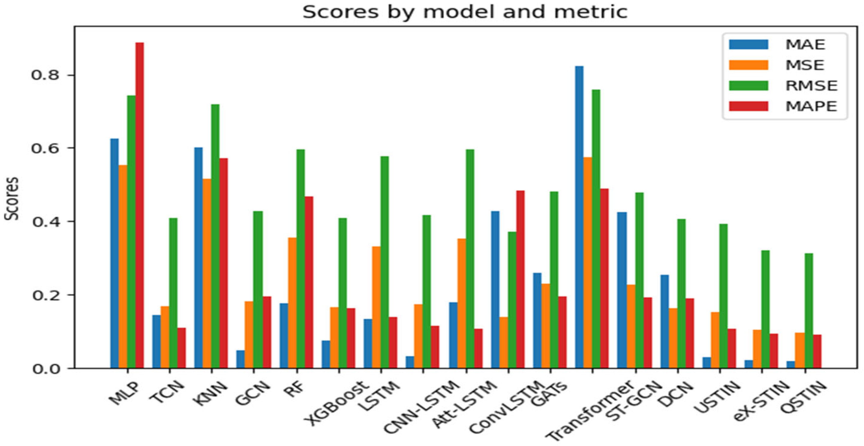
4.4. Evaluation Metrics

We used four standard evaluation metrics to assess prediction accuracy and enable comparison across different models applied to the same dataset [48].

4.4.1. Mean Absolute Error (MAE)

MAE represents the average of absolute prediction errors. It provides a clear measure of prediction error magnitude, independent of the error’s direction [49].

$$MAE=mean\left(absolute\left({expected}_{value}-{predicted}_{value}\right)\right)$$

(29)

4.4.2. Mean Square Error (MSE)

MSE calculates the average of the squared differences between predicted and actual values, offering an error measure that increases with the magnitude of the deviation [50].

$$MSE=mean\left({\left({expected}_{value}-{predicted}_{value}\right)}^2\right)$$

(30)

4.4.3. Root Mean Square Error (RMSE)

MSE penalizes larger prediction errors more heavily than MAE, making it particularly sensitive to significant deviations between predicted and actual values [50].

$$RMSE=sqrt\left(MSE\right)$$

(31)

4.4.4. Mean Absolute Percentage Error (MAPE)

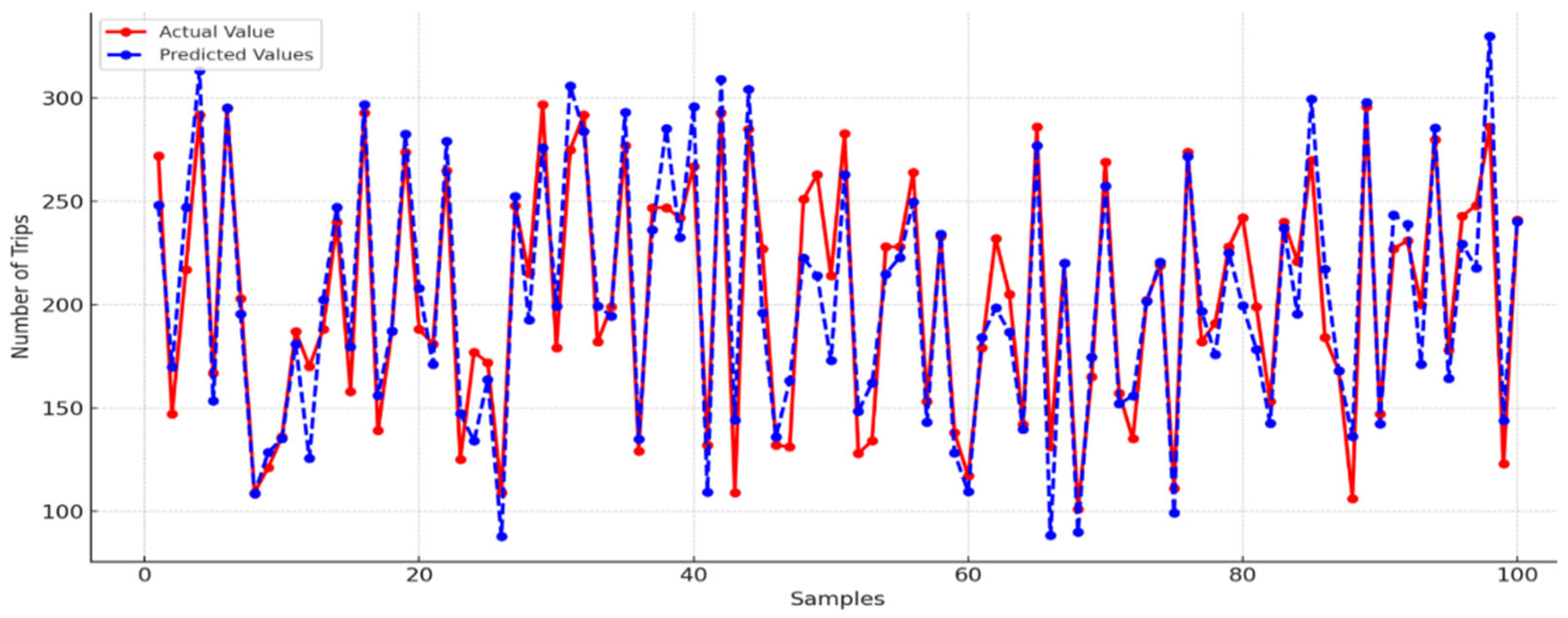
MAPE represents the average of absolute percentage errors between predicted and actual values, making it useful for interpreting model accuracy across datasets with different scales [51].

$$MAPE={\displaystyle \frac{100}{n}}\sum _{t=1}^n\left|{\displaystyle \frac{{expected}_{value}-{predicted}_{value}}{{expected}_{value}}}\right|$$

(32)

where:

$n$: the number of fitted points.

5. Discussion

This study aims to improve predictive accuracy in car-sharing demand prediction by leveraging quantum-inspired principles. The proposed model combines both QINN to capture complex interdependencies within multimodal urban data and QPSO in the final regression layer to optimize its parameters. We evaluated QSTIN against multiple baseline models, including its predecessor, using different evaluation metrics.

Table 4. Comparative evaluation of the proposed QSTIN model against traditional, deep learning, and spatio-temporal baseline models using four evaluation metrics.

	MAE	MSE	RMSE	MAPE
MLP	0.626	0.554	0.744	0.887
TCN	0.145	0.168	0.410	0.109
KNN	0.601	0.515	0.718	0.571
GCN	0.048	0.182	0.427	0.195
RF	0.177	0.356	0.597	0.469
XGBoost	0.076	0.167	0.409	0.164
LSTM	0.135	0.333	0.577	0.139
CNN-LSTM	0.033	0.175	0.418	0.115
Att-LSTM	0.181	0.354	0.595	0.108
ConvLSTM	0.428	0.139	0.373	0.484
GATs	0.259	0.230	0.480	0.195
Transformer	0.824	0.575	0.758	0.488
ST-GCN	0.426	0.229	0.479	0.192
DCN	0.255	0.165	0.406	0.191
USTIN	0.031	0.154	0.392	0.108
eX-STIN	0.022	0.104	0.322	0.094
Proposed (QSTIN)	0.020	0.098	0.313	0.078

presents the results of these comparisons, highlighting the smallest errors in bold text to indicate the best-performing model.

The QSTIN model achieved substantial performance improvements across a wide range of baseline and advanced models. Compared to traditional models, such as MLP, QSTIN achieved reductions of over 57% in RMSE and 91% in MAPE, indicating strong error minimization. Against temporal models, such as TCN, it demonstrated improvements of 23% in RMSE and 28% in MAPE, highlighting its ability to better capture sequential dynamics through complex-valued feature encoding.

Additional comparisons confirm that QSTIN consistently outperformed traditional machine learning models. It achieved RMSE reductions of 56% over KNN, 47% over RF, 37% over XGBoost, and 8% over GCN. These improvements underscore the model’s strength in handling nonlinear dependencies and irregular spatial patterns and multimodal feature interactions—areas where traditional models often underperform due to reliance on real-valued encodings.

Beyond traditional models, QSTIN also outperformed several deep learning architectures. For instance, compared to ConvLSTM, ST-GCN, DCN, and transformer, QSTIN achieved RMSE reductions of 16%, 58%, 22%, and 58%, respectively. Improvements over GATs and attention-based LSTM further confirm QSTIN’s superior ability to model complex spatio-temporal relationships. This performance is largely attributed to the integration of QINN and QPSO, which jointly enable robust representation learning and globally optimized convergence, respectively.

When compared to structurally similar models, QSTIN continued to demonstrate competitive advantages. It achieved a 36% improvement in MSE, a 20% reduction in RMSE, and a 28% gain in MAPE over the unified spatio-temporal inference network (USTIN) [7], which shares the same spatio-temporal inference foundation. Furthermore, relative to eX-STIN, QSTIN achieved additional reductions of 6% in MSE, 3% in RMSE, and 2% in MAPE. These results validate the impact of quantum-inspired refinements in predictive modeling frameworks.

Figure 3 illustrates the comparison between the predicted and actual car-sharing demand using the QSTIN model. The close alignment between the two curves demonstrates the model’s effectiveness in capturing temporal trends, spatial variations, and spatio-temporal dependencies, resulting in accurate predictions of demand fluctuations.

Figure 4 showcases the comparative performance analysis across multiple models using evaluation metrics. The results demonstrate that the proposed QSTIN model achieves the lowest error rates across all metrics, outperforming traditional baselines and advanced architectures, including USTIN and eX-STIN.

Figure 5 illustrates the RMSE convergence of the USTIN, eX-STIN, and QSTIN models over 100 training epochs, all of which are based on a common spatio-temporal inference architecture. QSTIN demonstrates superior training performance by integrating QINN within the fusion module, enabling complex-valued representation learning that captures intricate spatio-temporal dependencies more effectively. Moreover, the selective application of QPSO to the final output layer further accelerates convergence speed and prediction stability.

The main objective of this study is to enhance the predictive accuracy of car-sharing demand prediction by extending a spatio-temporal inference framework with quantum-inspired methodologies. The integration of the QINN within the fusion module enables the model to learn more expressive and complex feature representations. Unlike traditional models that rely on real-valued transformations, QINN leverages complex-valued encoding to capture higher-order correlations across temporal, spatial, and spatio-temporal dimensions. This enriched representation significantly improves the model’s ability to uncover nonlinear, entangled patterns in multimodal data, which are typically missed by conventional architectures. The empirical relevance of QINN is supported by previous research; Tomal et al. [29] demonstrated that quantum state encoding enhances classification accuracy in non-stationary time series, while Thakkar et al. [30] showed that QINNs effectively capture complex dependencies in financial prediction tasks. These findings affirm the suitability of QINN for high-dimensional, dynamic domains, such as urban mobility.

In addition, QPSO is applied at the final regression layer to improve global hyperparameter tuning. This further strengthens the model by improving convergence behavior and reducing the likelihood of being trapped in local optima. Huang et al. [52] illustrated that QPSO enhances convergence speed, while maintaining effective search capability, making it well-suited for real-time and resource-constrained applications. Al-Baity et al. [53] extended QPSO to multi-objective optimization and demonstrated its ability to explore complex solution spaces effectively.

The integration of QINN for enriched feature learning and QPSO for efficient global optimization represents a substantial improvement over conventional methods. Together, these components increase the model’s prediction accuracy and enable better generalization across varying temporal, spatial, and spatio-temporal conditions.

6. Conclusions

This study presents the quantum-inspired spatio-temporal inference network (QSTIN), a novel framework developed to address key limitations in conventional car-sharing demand prediction models. QSTIN enhances spatio-temporal learning by refining the fusion module through the integration of a quantum-inspired neural network (QINN), which enables the model to capture richer feature representations and uncover higher-order nonlinear interdependencies across temporal, spatial, and spatio-temporal dimensions. These relationships are often overlooked by traditional fusion architecture. In addition, quantum particle swarm optimization (QPSO) is selectively applied at the final regression layer to improve predictive precision through global parameter tuning, while preserving computational efficiency.

Experimental results demonstrate that QSTIN outperforms a wide range of baseline models across multiple evaluation metrics. Compared to its predecessor, eX-STIN, QSTIN achieves further accuracy gains by leveraging quantum-inspired learning and optimization strategies within the spatio-temporal inference process. These enhancements validate QSTIN’s ability to generalize effectively across complex and multimodal prediction scenarios. By advancing the predictive accuracy and generalization capacity of demand forecasting models, QSTIN contributes to the development of more adaptive and intelligent mobility systems. Accurate car-sharing demand prediction enables data-driven strategies for resource allocation and operational planning, which are essential for reducing inefficiencies, minimizing idle fleet distribution, and supporting sustainable urban transportation.

Despite its strong performance, QSTIN has two limitations that warrant further investigation. First, the model assumes consistent access to high-quality multimodal sensor data, which may not always be available in real-world urban settings. Second, while QPSO enhances convergence efficiency, the model’s responsiveness to rapidly evolving demand dynamics remains an open challenge. Future research will explore reinforcement learning-based adaptation and extend QSTIN’s applicability across broader domains in intelligent transportation and infrastructure planning.

References

1. Liang, Y.; You, J.; Wang, R.; Qin, B.; Han, S. Urban Transportation Data Research Overview: A Bibliometric Analysis Based on CiteSpace. Sustainability 2024, 16, 9615. [Google Scholar] [CrossRef]
2. Brahimi, N.; Zhang, H.; Razzaq, Z. Explainable Spatio-Temporal Inference Network for Car-Sharing Demand Prediction. ISPRS Int. J. Geo-Inf. 2025, 14, 163. [Google Scholar] [CrossRef]
3. Schuld, M.; Sinayskiy, I.; Petruccione, F. The quest for a Quantum Neural Network. Quantum Inf. Process. 2014, 13, 2567–2586. [Google Scholar] [CrossRef]
4. Beer, K.; Bondarenko, D.; Farrelly, T.; Osborne, T.J.; Salzmann, R.; Scheiermann, D.; Wolf, R. Training deep quantum neural networks. Nat. Commun. 2020, 11, 808. [Google Scholar] [CrossRef]
5. Sun, J.; Xu, W.; Feng, B. A global search strategy of Quantum-behaved Particle Swarm Optimization. In Proceedings of the 2004 IEEE Conference Cybernetics and Intelligent Systems, Singapore, 1–3 December 2004; pp. 111–116. [Google Scholar] [CrossRef]
6. Zouache, D.; Nouioua, F.; Moussaoui, A. Quantum-inspired firefly algorithm with particle swarm optimization for discrete optimization problems. Soft Comput. 2016, 20, 2781–2799. [Google Scholar] [CrossRef]
7. Brahimi, N.; Zhang, H.; Zaidi, S.D.A.; Dai, L. A Unified Spatio-Temporal Inference Network for Car-Sharing Serial Prediction. Sensors 2024, 24, 1266. [Google Scholar] [CrossRef]
8. Brahimi, N.; Zhang, H.; Dai, L.; Zhang, J. Modelling on Car-Sharing Serial Prediction Based on Machine Learning and Deep Learning. Complexity 2022, 8843000. [Google Scholar] [CrossRef]
9. Chen, L.; Chen, H. Joint distribution route optimization of vehicle and drone based on NSGA II. In Proceedings of the International Conference on Smart Transportation and City Engineering (STCE 2023), Chongqing, China, 16–18 December 2023; p. 109. [Google Scholar] [CrossRef]
10. Chai, X.; Zhang, Y.; Du, D.; Sun, Y. Bi-level optimization scheduling of electric vehicle-distribution network considering demand response and carbon quota. J. Phys. Conf. Ser. 2024, 2849, 012075. [Google Scholar] [CrossRef]
11. Luan, R. Logistics distribution route optimization of electric vehicles based on distributed intelligent system. Int. J. Emerg. Electr. Power Syst. 2024, 25, 629–639. [Google Scholar] [CrossRef]
12. Petri, M.; Kniess, J.; Parpinelli, R.S. Resource scheduling for mobility scenarios with time constraints. In Proceedings of the 2018 44th Latin American Computer Conference (CLEI 2018), Sao Paulo, Brazil, 1–5 October 2018; pp. 184–191. [Google Scholar] [CrossRef]
13. Hsieh, C.; Sani, A.; Dutt, N. The case for exploiting underutilized resources in heterogeneous mobile architectures. In Proceedings of the 2019 Design, Automation & Test in Europe Conference & Exhibition (DATE), Florence, Italy, 25–29 March 2019. [Google Scholar] [CrossRef]
14. Feng, S.; Ke, J.; Yang, H.; Ye, J. A Multi-Task Matrix Factorized Graph Neural Network for Co-Prediction of Zone-Based and OD-Based Ride-Hailing Demand. IEEE Trans. Intell. Transp. Syst. 2022, 23, 5704–5716. [Google Scholar] [CrossRef]
15. Wang, C.; Deng, Z. Multi-perspective Spatiotemporal Context-aware Neural Networks for Human Mobility Prediction. In Proceedings of the HuMob 2023—1st International Workshop on the Human Mobility Prediction Challenge, Hamburg, Germany, 13 November 2023; pp. 32–36. [Google Scholar] [CrossRef]
16. He, M.; Li, X.; Zhao, H.; Yao, Y.; Zhou, T. A Topology-Enhanced Graph Convolutional Network for Urban Traffic Prediction. In Proceedings of the 2024 7th International Conference on Electronics Technology, Chengdu, China, 17–20 May 2024; pp. 1093–1097. [Google Scholar] [CrossRef]
17. Yuan, G.; Fan, X.; Huang, Y.; Xuesong, J. Research on Urban Traffic Flow Prediction Model Utilizing Heterogeneous Data Fusion. In Proceedings of the 2024 10th IEEE International Conference on Intelligent Data and Security (IDS), New York City, NY, USA, 10–12 May 2024; pp. 32–36. [Google Scholar] [CrossRef]
18. Pan, Z.; Liang, Y.; Wang, W.; Yu, Y.; Zheng, Y.; Zhang, J. Urban traffic prediction from spatio-temporal data using deep meta learning. In Proceedings of the 25th ACM SIGKDD Conference on Knowledge Discovery and Data Mining, Anchorage, AK, USA, 4–8 August 2019; pp. 1720–1730. [Google Scholar] [CrossRef]
19. Yu, B.; Li, M.; Zhang, J.; Zhu, Z. 3D Graph Convolutional Networks with Temporal Graphs: A Spatial Information Free Framework for Traffic Forecasting. arXiv 2019, arXiv:1903.00919. [Google Scholar] [CrossRef]
20. Ou, J.; Sun, J.; Zhu, Y.; Jin, H.; Liu, Y.; Zhang, F.; Huang, J.; Wang, X. STP-TrellisNets+: Spatial-Temporal Parallel TrellisNets for Multi-Step Metro Station Passenger Flow Prediction. IEEE Trans. Knowl. Data Eng. 2023, 35, 7526–7540. [Google Scholar] [CrossRef]
21. Kardashin, A.; Balkybek, Y.; Palyulin, V.V.; Antipin, K. Predicting properties of quantum systems by regression on a quantum computer. Phys. Rev. Res. 2025, 7, 013201. [Google Scholar] [CrossRef]
22. Huerga, A.; Aguilera, U.; Almeida, A.; Lago, A.B. A Quantum Computing Approach to Human Behavior Prediction. In Proceedings of the 2022 7th International Conference on Smart and Sustainable Technologies, Bol, Croatia, 5–8 July 2022. [Google Scholar] [CrossRef]
23. Surendiran, B.; Dhanasekaran, K.; Tamizhselvi, A. A Study on Quantum Machine Learning for Accurate and Efficient Weather Prediction. In Proceedings of the 2022 Sixth International Conference on I-SMAC (IoT in Social, Mobile, Analytics and Cloud) (I-SMAC), Dharan, Nepal, 10–12 November 2022; pp. 534–537. [Google Scholar] [CrossRef]
24. Li, Q.; Huang, Z.; Jiang, W.; Tang, Z.; Song, M. Quantum Algorithms Using Infeasible Solution Constraints for Collision-Avoidance Route Planning. IEEE Trans. Consum. Electron. 2024. [Google Scholar] [CrossRef]
25. Zhuang, Y.; Azfar, T.; Wang, Y.; Sun, W.; Wang, X.; Guo, Q.; Ke, R. Quantum Computing in Intelligent Transportation Systems: A Survey. CHAIN 2024, 1, 138–149. [Google Scholar] [CrossRef]
26. Qu, Z.; Liu, X.; Zheng, M. Temporal-Spatial Quantum Graph Convolutional Neural Network Based on Schrödinger Approach for Traffic Congestion Prediction. IEEE Trans. Intell. Transp. Syst. 2023, 24, 8677–8686. [Google Scholar] [CrossRef]
27. Pandurangan, K.; Priyadharshini, A.; Taseen, R.; Galebathullah, B.; Yaseen, H.; Ravichandran, P. Quantum-Inspired Algorithms for AI and Machine Learning. In Integration of AI, Quantum Computing, and Semiconductor Technology; IGI Global: Hershey, PA, USA, 2024; pp. 79–92. [Google Scholar] [CrossRef]
28. Zhang, B. Quantum Neural Networks: A New Frontier. Theor. Nat. Sci. 2024, 41, 122–128. [Google Scholar] [CrossRef]
29. Tomal, S.M.Y.I.; Al Shafin, A.; Afaf, A.; Bhattacharjee, D. Quantum Convolutional Neural Network: A Hybrid Quantum-Classical Approach for Iris Dataset Classification. J. Future Artif. Intell. Technol. 2024, 1, 284–295. [Google Scholar] [CrossRef]
30. Thakkar, S.; Kazdaghli, S.; Mathur, N.; Kerenidis, I.; Ferreira–Martins, A.J.; Brito, S. Improved financial forecasting via quantum machine learning. Quantum Mach. Intell. 2024, 6, 27. [Google Scholar] [CrossRef]
31. Dong, Y.; Xie, J.; Hu, W.; Liu, C.; Luo, Y. Variational algorithm of quantum neural network based on quantum particle swarm. J. Appl. Phys. 2022, 132, 104401. [Google Scholar] [CrossRef]
32. Alvarez-Alvarado, M.S.; Alban-Chacón, F.E.; Lamilla-Rubio, E.A.; Rodríguez-Gallegos, C.D.; Velásquez, W. Three novel quantum-inspired swarm optimization algorithms using different bounded potential fields. Sci. Rep. 2021, 11, 11655. [Google Scholar] [CrossRef] [PubMed]
33. Fallahi, S.; Taghadosi, M. Quantum-behaved particle swarm optimization based on solitons. Sci. Rep. 2022, 12, 13977. [Google Scholar] [CrossRef] [PubMed]
34. Zhang, D.; Wang, J.; Fan, H.; Zhang, T.; Gao, J.; Yang, P. New method of traffic flow forecasting based on quantum particle swarm optimization strategy for intelligent transportation system. Int. J. Commun. Syst. 2021, 34, e4647. [Google Scholar] [CrossRef]
35. Sengupta, S.; Basak, S.; Peters, R.A. Data Clustering using a Hybrid of Fuzzy C-Means and Quantum-behaved Particle Swarm Optimization. In Proceedings of the 2018 IEEE 8th Annual Computing and Communication Workshop and Conference (CCWC), Las Vegas, NV, USA, 8–10 January 2018; pp. 137–142. [Google Scholar] [CrossRef]
36. Mao, X.; Yang, A.C.; Peng, C.K.; Shang, P. Analysis of economic growth fluctuations based on EEMD and causal decomposition. Phys. A Stat. Mech. Its Appl. 2020, 553, 124661. [Google Scholar] [CrossRef]
37. Li, Z.; Jiang, Y.; Hu, C.; Peng, Z. Recent progress on decoupling diagnosis of hybrid failures in gear transmission systems using vibration sensor signal: A review. Measurement 2016, 90, 4–19. [Google Scholar] [CrossRef]
38. Zhang, Y.; Ding, C.; Li, T. Gene selection algorithm by combining reliefF and mRMR. BMC Genom. 2008, 9 (Suppl. S2), S27. [Google Scholar] [CrossRef]
39. Ardiles, L.G.; Tadano, Y.S.; Costa, S.; Urbina, V.; Capucim, M.N.; da Silva, I.; Braga, A.; Martins, J.A.; Martins, L.D. Negative Binomial regression model for analysis of the relationship between hospitalization and air pollution. Atmos. Pollut. Res. 2018, 9, 333–341. [Google Scholar] [CrossRef]
40. Zhang, K.; Zhang, Y.; Wang, M. A Unified Approach to Interpreting Model Predictions Scott. Nips 2012, 16, 426–430. [Google Scholar]
41. Ahmed, S.F.; Bin Alam, S.; Hassan, M.; Rozbu, M.R.; Ishtiak, T.; Rafa, N.; Mofijur, M.; Ali, A.B.M.S.; Gandomi, A.H. Deep learning modelling techniques: Current progress, applications, advantages, and challenges. Artif. Intell. Rev. 2023, 56, 13521–13617. [Google Scholar] [CrossRef]
42. Guidotti, R.; Monreale, A.; Ruggieri, S.; Turini, F.; Giannotti, F.; Pedreschi, D. A survey of methods for explaining black box models. ACM Comput. Surv. 2018, 51, 93. [Google Scholar] [CrossRef]
43. Zhao, Q.; Hou, C.; Xu, R. Quantum-inspired complex-valued language models for aspect-based sentiment classification. Entropy 2022, 24, 621. [Google Scholar] [CrossRef] [PubMed]
44. Shi, S.; Wang, Z.; Cui, G.; Wang, S.; Shang, R.; Li, W.; Wei, Z.; Gu, Y. Quantum-inspired complex convolutional neural networks. Appl. Intell. 2022, 52, 17912–17921. [Google Scholar] [CrossRef]
45. Caragea, A.; Lee, D.G.; Maly, J.; Pfander, G.; Voigtlaender, F. Quantitative Approximation Results for Complex-Valued Neural Networks. SIAM J. Math. Data Sci. 2022, 4, 553–580. [Google Scholar] [CrossRef]
46. Liu, L.; Fan, X. An Improved Quantum Particle Swarm Optimization Algorithm for Target Tracking Deployment in Spatial Sensor Networks. J. Internet Technol. 2024, 25, 709–721. [Google Scholar] [CrossRef]
47. Zamani Joharestani, M.; Cao, C.; Ni, X.; Bashir, B.; Talebiesfandarani, S. PM2.5 Prediction Based on Random Forest, XGBoost, and Deep Learning Using Multisource Remote Sensing Data. Atmosphere 2019, 10, 373. [Google Scholar] [CrossRef]
48. Chen, C.; Twycross, J.; Garibaldi, J.M. A new accuracy measure based on bounded relative error for time series forecasting. PLOS ONE 2017, 12, e0174202. [Google Scholar] [CrossRef]
49. Chicco, D.; Warrens, M.J.; Jurman, G. The coefficient of determination R-squared is more informative than SMAPE, MAE, MAPE, MSE and RMSE in regression analysis evaluation. PeerJ Comput. Sci. 2021, 7, e623. [Google Scholar] [CrossRef]
50. Hosamo, H.; Mazzetto, S. Performance Evaluation of Machine Learning Models for Predicting Energy Consumption and Occupant Dissatisfaction in Buildings. Buildings 2024, 15, 39. [Google Scholar] [CrossRef]
51. Kim, S.; Kim, H. A new metric of absolute percentage error for intermittent demand forecasts. Int. J. Forecast. 2016, 32, 669–679. [Google Scholar] [CrossRef]
52. Huang, Z.; Wang, Y.; Yang, C.; Wu, C. A new improved quantum-behaved particle swarm optimization model. In Proceedings of the 2009 4th IEEE Conference on Industrial Electronics and Applications (ICIEA 2009), Xi’an, China, 25–27 May 2009; pp. 1560–1564. [Google Scholar] [CrossRef]
53. AlBaity, H.; Meshoul, S.; Kaban, A. On extending quantum behaved particle swarm optimization to multiobjective context. In Proceedings of the 2012 IEEE Congress on Evolutionary Computation (CEC 2012), Brisbane, QLD, Australia, 10–15 June 2012. [Google Scholar] [CrossRef]
Figure 1. Architecture of the quantum-inspired spatio-temporal inference network (QSTIN).
Sustainability 17 04987 g001
Figure 2. Temporal fusion network (TFN) architecture used for extracting multiscale temporal patterns, comprising TCN encoding, attention mechanism, and LSTM decoding [2].
Sustainability 17 04987 g002
Figure 3. Predicted vs. actual car-sharing demand using the QSTIN model across a selected range of time intervals. The red line represents actual demand, while the blue line indicates the model’s predicted values.
Sustainability 17 04987 g003
Figure 4. Comparative evaluation of QSTIN and baseline models across multiple evaluation metrics. The figure illustrates QSTIN’s consistently superior performance, reflected by lower prediction errors compared to traditional machine learning models, deep learning architectures, and spatio-temporal inference frameworks.
Sustainability 17 04987 g004
Figure 5. RMSE convergence trends over training epochs for USTIN, eX-STIN, and QSTIN models, showing that QSTIN achieves faster and more stable convergence. This reflects the effectiveness of quantum-inspired optimization in accelerating learning and improving model stability during training.
Sustainability 17 04987 g005