Article

Numerical Modeling of Biofilm–Flow Dynamics in Gravel-Bed Rivers: A Framework for Sustainable Restoration

1
Nanxun Innovation Institute, Zhejiang University of Water Resources and Electric Power, Hangzhou 310000, China
2
Qingyuan County Water Resources Bureau, Hangzhou 310000, China
*
Author to whom correspondence should be addressed.
Sustainability 2025, 17(11), 4905; https://doi.org/10.3390/su17114905
Submission received: 26 April 2025 / Revised: 18 May 2025 / Accepted: 22 May 2025 / Published: 27 May 2025
(This article belongs to the Special Issue Hydrosystems Engineering and Water Resource Management)

Abstract

:
This study investigates biofilm–flow interactions in gravel-bed rivers using a novel numerical model. Traditional hydrodynamic models often overlook biofilm-induced roughness coupling, prompting the development of a mesoscopic Lattice Boltzmann Method (LBM) framework that dynamically links biofilm thickness to equivalent roughness. Key insights include a dual-phase mechanism: moderate biofilm growth reduces hydraulic resistance by smoothing gravel pores, while excessive growth increases resistance via flow obstruction. Validated against 65-day flume experiments, the model accurately predicted biomass (ash-free dry mass) and velocity profiles. Current limitations involve reliance on empirical biofilm formulas, lack of natural river validation (non-uniform substrates, dynamic flows), and computational barriers in 3D large-scale simulations. Future directions include integrating biogeochemical factors (temperature, nutrients), multiscale microbial-morphology frameworks, and GPU-accelerated high-resolution modeling.

1. Introduction

River hydrodynamics serve as a crucial environmental factor governing both contaminant transport and water quality [1]. Sustainable management of riverine ecosystems is critical for addressing global challenges such as water scarcity and pollution. Gravel-bed rivers, as a representative fluvial morphology, provide ideal colonization spaces for microbial communities through their abundant porous structures. Notably, biofilm development can significantly alter hydraulic characteristics within channels [2]. Therefore, investigating the interaction mechanisms between biofilm and hydrodynamics in gravel-bed rivers holds substantial guidance value for optimizing ecological restoration projects in such aquatic systems [3].
Gravel-bed rivers (GBRs), prevalent in mountainous and alluvial plain environments, exhibit distinct hydrodynamic properties and bed roughness characteristics that profoundly govern flow resistance distribution, sediment transport regimes, and ecological functionality. Studies have demonstrated that rough gravel beds alter flow structures through dual-scale mechanisms: at the microscale, surface friction induced by discrete particles amplifies near-bed velocity gradients [4]; at the macroscale, bedform geometry triggers flow separation, leading to significant heterogeneity in vertical velocity distribution [5]. These coupled mechanisms constitute the core components of total resistance coefficients—surface friction and form drag, with the latter arising from bedform-induced flow separation, turbulent bursting, and energy dissipation processes [6]. Experimental hydrodynamics reveals the dominance of form drag: when the D50 particle size exceeds a critical threshold (typically >5 mm), form drag contributes 60–80% of the total bed shear stress [7]. High-resolution PIV measurements confirm that gravel protrusions and spatial arrangements induce periodic shedding of horseshoe vortices and wake vortices, with these coherent structures significantly enhancing turbulent kinetic energy production and dissipation [8]. Notably, van der Mark et al. [9] demonstrated through variable-slope flume experiments that when the width-to-depth ratio (B/H) exceeds 20, the contribution of bedforms to resistance coefficients decays exponentially, although abrupt bedform transitions downstream can provoke localized resistance surges exceeding 40%. Biofilm colonization can elevate roughness values by 1.5–2 times baseline levels [10]. Through controlled flume experiments, they developed an empirical model linking biofilm thickness to Manning’s coefficient. Advanced investigations further uncover hydrodynamic-biofilm interactions: beyond critical velocities (~0.8 m/s), elevated shear stresses induce biofilm sloughing. This dynamic equilibrium modulates flow resistance through continuous adjustments of equivalent roughness height, governed by biofilm structural parameters including hyphal density and porosity [11].
Numerical modeling has emerged as a pivotal tool in fluvial hydrodynamics research, providing cost-effective alternatives to physical experiments, while enabling high-resolution analysis of flow mechanisms across spatiotemporal scales [12,13,14]. Contemporary hydrodynamic simulations predominantly employ three classical discretization frameworks: (1) Finite Volume Method (FVM) excels in mass conservation for open-channel flows, making it the cornerstone of industrial-standard software like ANSYS Fluent V6.3 and MIKE 21 series [15,16]; (2) Finite Element Method (FEM) demonstrates superior adaptability in handling irregular bathymetry through flexible mesh generation, as implemented in TELEMAC-MASCARET [17]; (3) Finite Difference Method (FDM) remains prevalent in large-scale river network modeling due to its computational efficiency, exemplified by HEC-RAS [18]. The past decade has witnessed a paradigm shift toward mesoscopic approaches, particularly Lattice Boltzmann Method (LBM), which resolves flow fields through kinetic theory-based particle interactions [19]. Unlike continuum-based methods, LBM inherently accommodates complex boundaries (e.g., boulder clusters, vegetation canopies) without explicit interface tracking algorithms [20]. Case studies reveal LBM’s exceptional performance in scenarios where traditional methods falter.
This study conducts an in-depth investigation into the theoretical limitations of traditional hydrodynamic modeling for gravel-bed channels. While existing models have incorporated the influence mechanisms of gravel substrate roughness on flow dynamics, they fail to effectively characterize the coupling effects of biofilm dynamic evolution processes on channel bed boundary conditions. Notably, there remains a lack of systematic research on the spatiotemporal growth patterns of biofilms and their modulation mechanisms on channel roughness parameters, which constitutes a critical scientific challenge constraining the improvement of predictive accuracy in hydrodynamic models. To address this, the study innovatively develops a hydrodynamic numerical model for gravel-bed slopes that integrates biofilm growth effects, by synthesizing multi-source experimental observations and theoretical analysis methods. The research employs the Lattice Boltzmann Method (LBM) to establish the numerical computation framework, leveraging its mesoscopic modeling advantages to effectively capture microscopic flow characteristics at complex solid–liquid interfaces. Through establishing a dynamic correlation model between biofilm thickness and roughness parameters, the study successfully achieves refined simulation of hydrodynamic characteristics in channels across different stages of biofilm lifecycles. The developed modeling methodology not only addresses the theoretical deficiencies of conventional models, but also establishes a new numerical experimental platform for investigating hydrodynamic properties in ecological river systems, thereby providing theoretical foundations and technical support for relevant engineering practices. By elucidating biofilm-mediated hydrodynamic interactions, this study bridges the gap between ecological restoration and hydraulic engineering, offering a pathway to optimize river management for both environmental sustainability and human needs.

2. Materials and Methods

2.1. Numerical Model

2.1.1. Hydraulic Model

The Lattice Boltzmann Method (LBM) offers unique advantages for sustainable hydrology. Unlike conventional CFD methods, LBM efficiently simulates multi-scale interactions between biofilm microstructure and macro-scale flow patterns [21]. This capability is critical for predicting long-term ecological outcomes, such as how biofilm succession under climate change scenarios (e.g., intensified droughts) alters river resilience.
For hydrodynamic simulations in gravel-bedded channels, the channel can be divided into two zones: the gravel layer and the flow layer. The primary distinction between the governing equations for these two zones lies in the drag force terms. As shown in Equation (1), the flow resistance in the flow layer primarily originates from the bed roughness, while the flow resistance in the gravel layer mainly arises from the drag forces generated by both the gravels and biofilms.
u i t + u i u j t = ν + ν e 2 u i x j x j g z b x i S b i   Flow   layer u i t + u i u j t = ν + ν e 2 u i x j x j g z b x i F s F b   Gravel   Layer
where the Einstein summation convention over lattice indices is adopted; t denotes the time; u i is the velocity; ν and ν e represent kinematic and eddy viscosity, respectively; and z b is the bed elevation; F s is the volumetric force generated by porous materials; and F b is the volumetric force generated by biofilm.
S b i is the bed shear stress term in the i direction and expressed as a Manning formula
S b i = g n s 2 h 1 / 3 u i u j u j
where n s refers to Manning’s coefficient and h is the water depth.
As shown in Figure 1a, the bed roughness coefficient is solely governed by the intrinsic roughness of the gravel substrate prior to biofilm colonization. During biofilm development, the roughness coefficient exhibits significant correlation with biofilm development. Experimental studies demonstrate a dual-phase modulation mechanism: (i) In gravel-bed channels, moderate biofilm colonization fills interstitial pores between substrate particles (Figure 1b), effectively smoothing the bed surface and consequently reducing hydraulic roughness. (ii) However, when biofilm accumulation exceeds critical thickness thresholds surpassing gravel protrusions (Figure 1c), it initiates flow obstruction through emergent biological structures, thereby augmenting overall roughness. This nonlinear relationship suggests that bed roughness constitutes a composite function of intrinsic substrate roughness and dynamic biofilm thickness parameters.
n s = n + κ γ γ s 2
where n denotes the roughness coefficient of biofilm-free gravel-bed substrate, κ represents the constant coefficient, and γ s signifies the critical width of biofilm for gravel-bed channels.
The bed roughness coefficient of gravel-bed channels correlates with the characteristic particle diameter D 50 , which can be mathematically represented by the following governing equation [22]
n = 0.59 D 50 0.179
Regarding the flow resistance exerted by gravel substrates, we conceptualize this phenomenon as rigid vegetation with variable diameters following Huai et al. [23]. For biofilm-colonized gravels, biological growth is assumed to effectively increase the equivalent gravel thickness (Figure 2). This modification leads to the reformulated governing equation.
S f i = 1 2 C D a u i 2
where C D is the coefficient of the rigid vegetation which can be assumed as 1 [24], a is the vegetation density coefficient and a = α × d + 2 d b , d is the diameter of vegetation, α is the vegetation number per m2, and  d b is the width of biofilm.
The LBM has emerged as a well-established computational framework for simulating hydrodynamic processes in both open-channel flows and porous media systems, as evidenced by recent advancements in the field [25]. Building upon this methodological foundation, the present study employs LBM to resolve the velocity distribution characteristics inherent to gravel-bed flow dynamics. At its core, the LBM algorithm operates through two sequential, particle-based computational phases: (1) collision processes governing microscopic momentum redistribution and (2) streaming (propagation) mechanisms dictating mesoscopic particle transport. These fundamental operations are mathematically formalized through the following governing equations
f ε x + e ε t ,   t + t = f ε x ,   t 1 τ t f ε x ,   t f ε e q x ,   t + t N ε e 2 e ε i F i
where f ε represents the distribution function of particles; f e q is the local equilibrium distribution function; x is the space vector in Cartesian coordinates; e = x / t ; x is the lattice size; t is the time step; τ t is the total relaxation time parameter; and F i denotes the external forces.
N ε is a constant that can be defined as follows:
N ε = 1 e 2 ε e ε i e ε i
This study employs the widely recognized D2Q9 lattice configuration of the Discrete Boltzmann Model (Figure 3) to simulate two-dimensional hydrodynamic systems, consistent with established numerical frameworks [26,27]. Within this computational paradigm, the discrete velocity set e ε , a fundamental component governing particle dynamics in the D2Q9 scheme, is mathematically defined as follows.
e ε = 0 ,   0 ,   ε = 0 e c o s α 1 π 4 , s i n α 1 π 4   ,   ε = 1 ,   2 ,   3 ,   4 2 e c o s α 1 π 4 , s i n α 1 π 4   ,   ε = 5 ,   6 ,   7 ,   8
The local equilibrium distribution function f e q in the lattice Boltzmann framework is formulated as
f ε e q = 1 5 g 6 e 2 2 3 e 2 u i u i ,   ε = 0 g 6 e 2 + 1 3 e 2 e ε i u i + 1 2 e 4 e ε i e ε j u i u j 1 6 e 2 u i u i ,   ε = 1 ,   2 ,   3 ,   4 g 24 e 2 + 1 12 e 2 e ε i u i + 1 8 e 4 e ε i e ε j u i u j 1 24 e 2 u i u i ,   ε = 5 ,   6 ,   7 ,   8
The relaxation time parameter τ t , which governs the rate of approach to local equilibrium in lattice Boltzmann simulations, can be determined using the formulation proposed by Liu et al. [28]
τ t = τ + τ 2 + 18 C s 2 / e 2 i j i j 1
i j = ε e ε i e ε j f α f α e q
where τ denotes the single-relaxation time and C s is the Smagorinsky constant.
The external force components F ε i , accounting for momentum exchange mechanisms within the coupled fluid-vegetation system, are formulated separately for the hydrodynamic boundary layer (Flow Layer) and vegetative canopy region (Gravel Layer) through the following
F ε i = g z b x i g n 2 h 1 3 u i u j u j   Flow   layer F ε i = g z b x i 1 2 C D a u i 2   Gravel   Layer
The external force term is numerically evaluated through midpoint quadrature integration, spatially discretized at the geometric centroid between adjacent lattice nodes in the computational domain, as
F ε i = F ε i x i + 1 2 e ε i t ,   t

2.1.2. Biofilm Growth and Detachment Model

The traditional approach employs the Monod model to simulate biofilm dynamics [29]. The Monod equation regulates the microbial specific growth rate through substrate concentration, emphasizing the dominant role of external substrate limitation; however, it does not account for the influence of flow velocity on biofilm formation. Graba et al. [30] proposed a model that replaces substrate limitation with a self-inhibition term based on biomass density, reflecting the inhibitory effects of internal spatial competition or metabolic byproduct accumulation within biofilms (Equation (14)). This approach is more applicable to open systems where substrates are abundant, but physical space is constrained. Additionally, this model innovatively introduces a detachment term linearly correlated with hydraulic shear intensity and the roughness Reynolds number, directly coupling hydrodynamic conditions with biofilm dynamics. This addresses the limitation of the Monod model, which focuses solely on growth, while neglecting physical detachment processes. This improvement enables the model to dynamically characterize the equilibrium mechanism between biofilm growth and detachment, providing a more comprehensive theoretical framework for simulating biofilm-mediated ecological processes in complex flow fields.
d B d t = μ m a x B 1 1 + k i n v B C d e t k + B
where C d e t (s/m3/d) is an empirical detachment coefficient, and k + (m3/s) is the Roughness Reynolds number, t (days) is the time, μ m a x (d−1) is the maximum specific growth rate at the reference temperature 20 °C, k i n v (m2/g) is the inverse half-saturation constant for biomass.
The parameters of Equation (15) are given as Table 1.

2.1.3. Error Analysis

Error analysis was conducted to determine the difference between the predicted and measured data. The coefficient of determination R 2 were calculated by the following equations
R 2 = 1 S S E S S T ,
S S T = i = 1 N ( Y i m e a n Y ) 2 ,
S S E = i = 1 N ( Y i X i ) 2 ,
m e a n Y = 1 N i = 1 N Y i ,
where N is the number of lateral measuring points, and X and Y are the calculated and measured values.
The specific steps of the numerical model are illustrated in Figure 4 below. First, set initial conditions such as water depth and flow velocity, and initialize grid division and relaxation variables. Subsequently, simulate fluid motion through particle migration, calculate biofilm width and external forces using governing equations, then redistribute particles and update the distribution function. These steps are cyclically executed until reaching the preset time, after which the results are output.

2.2. Validation Data

The validation data in this study were sourced from Graba et al. [30]. The experiment was conducted in an indoor recirculating flume (Figure 5) measuring 11 m in length, 0.5 m in width, and 0.2 m in depth, with artificial cobblestones (37 mm diameter, 20 mm height) laid on the bottom to simulate a natural gravel riverbed. Under constant discharge (~14.4 m3/s) and channel slope (10−3), water flow was regulated through a partial recirculation system using filtered river water to exclude suspended matter and predators. Illumination was provided by fluorescent daylight and red light lamps (16 h light/8 h dark photoperiod) to maintain photosynthetically saturating light conditions (140–180 μmol m−2 s−1 PAR). Epilithic biofilms collected from natural streams were homogenized into suspensions and inoculated into the flume. The experiment comprised two phases: an inoculation period (3 weeks under closed circulation) and a growth period (65 days under open circulation). Ten cobblestones were randomly sampled weekly, with 6 specimens analyzed for ash-free dry mass (AFDM) and 4 for chlorophyll-a (Chl-a) quantification. AFDM was determined through drying-combustion methods, while Chl-a was extracted using spectrophotometric techniques. Weekly microscopic examinations were performed to identify dominant algal species in selected samples.

3. Results

The biomass results are shown in Figure 6. The trend of AFDM reveals that during the initial experimental phase (0–10 days), the biomass rapidly increased from the baseline to approximately 20 g/m2, reaching a peak (25–30 g/m2) around day 15. This accumulation occurred under relatively high roughness Reynolds numbers (a dimensionless parameter reflecting flow-bed roughness interactions), which initially enhanced turbulence and nutrient transport, facilitating biofilm growth. However, during the mid-phase (15–20 days), the roughness Reynolds number decreased, corresponding to a stabilization of hydrodynamic shear stress and the observed biomass peak. Subsequently, as the experiment progressed (20–30 days), the roughness Reynolds number increased again due to intensified flow velocity, leading to elevated hydraulic shear forces that triggered significant biofilm detachment. By the end of the experiment, the biomass declined to 15–20 g/m2. The temporal alignment of AFDM dynamics with the roughness Reynolds number—high (early), low (mid), and high (late)—underscores its pivotal role in governing biomass accumulation and loss. Specifically, high Reynolds numbers initially promoted growth but later exacerbated detachment, while the mid-phase low values allowed temporary stability [30]. This bidirectional relationship highlights hydrodynamic conditions as the key driver of biomass heterogeneity.
The simulation results of flow velocity are shown in Figure 7, and the simulated flow velocity exhibits good agreement. As observed in the figure, the flow velocity in the gravel zone is initially higher because the porosity of the gravel is at its maximum during this stage. Over time, as the biofilm begins to grow, the flow velocity in the gravel zone decreases significantly, as the increased biofilm reduces the porosity of the gravel. Concurrently, since the pores in the gravel are filled by the biofilm, the roughness decreases, leading to an increase in flow velocity within the water zone. Finally, excessive biofilm growth within the gravel causes the roughness of the gravel zone to rise again, at which point the flow velocity in the water zone begins to decline.

4. Discussion

4.1. Velocity Analysis

The study of hydrodynamic processes in traditional gravel-bed rivers has primarily focused on the velocity distribution characteristics within the open-channel flow zone, while relatively insufficient attention has been paid to hydrodynamic processes in the hyporheic layer [34]. This research bias stems from dual technical constraints: First, significant instrument penetration limitations exist in monitoring internal flow fields within gravel porous media, making it challenging for current measurement techniques to obtain reliable vertical velocity profile data [31,32,33,34]. Some studies have employed tracer methods to measure water residence time in porous media [35,36], yet these approaches fail to quantitatively characterize the vertical velocity distribution patterns within gravel layers. Second, the velocity magnitude in the hyporheic layer is typically 1–2 orders of magnitude lower than that of surface flow, often being regarded as a secondary influencing factor through dimensional analysis [37]. Consequently, mainstream numerical models frequently simplify gravel layers as fixed roughness boundary conditions. However, this simplified approach presents theoretical deficiencies: when applying zero-velocity boundary conditions (i.e., setting the top boundary velocity of the hyporheic layer as u = 0 m/s), even while maintaining constant bed slope and roughness parameters, the model outputs still exhibit systematic negative deviations in near-bed velocity fields [38]. The comparative study shown in Figure 7 demonstrates that by refining boundary condition settings (i.e., allowing continuous velocity transition at the hyporheic layer interface), simulation accuracy of near-bed flow fields can be significantly improved under identical roughness parameters.

4.2. Pollution Transport Analysis

Additionally, the flow velocity within the gravel layer exerts a dual regulatory role on pollutant transport processes. The porous gravel matrix inherently possesses pollutant adsorption capacity [39], while flow velocity not only governs the spatial distribution of dissolved contaminants in the hyporheic zone but also determines adsorption efficiency by modulating hydraulic retention time [40]. Specifically, reduced flow velocities enhance pollutant retention by prolonging water–sediment interactions, whereas accelerated flow may trigger adsorption–desorption dynamic equilibria under varying hydraulic gradients. The development of biofilm communities demonstrates coupled dependence on hydrodynamic conditions and contaminant transport dynamics [41]. Hydrodynamic shear stress regulates biofilm colonization patterns through nutrient transport efficiency while governing biofilm detachment mechanisms via mechanical scouring effects [2]. Simultaneously, pollutant fluxes serve dual functions as metabolic substrates for microbial communities and chemical inducers for extracellular polymeric substance (EPS) secretion [42]. This dual regulatory mechanism establishes a hydrodynamically modulated and chemically constrained biofilm-mediated biogeochemical cycle.

4.3. Limitation of This Study

4.3.1. Limited Field Data

The existing model was primarily validated using laboratory-based data (e.g., artificial gravel beds, constant flow rates), lacking adaptability testing in natural complex river channels (e.g., non-uniform substrates, dynamic flows), which may limit the generalizability of its practical engineering applications. The model relies on empirical formulas to describe biofilm growth and detachment, without fully considering the regulatory effects of environmental factors (e.g., temperature, light, dissolved oxygen, nutrient concentrations) on biofilm metabolic rates and structures, potentially leading to deviations in long-term simulations. The coupling mechanisms between biofilms and sediment transport or pollutant adsorption–desorption processes remain underexplored, particularly the unquantified feedback effects of biofilms on substrate stability and pollutant migration pathways. Although the LBM excels in handling complex boundaries, its high computational costs in three-dimensional large-scale simulations restrict its potential for long-term temporal or large spatial-scale applications. Validation data with limited temporal resolution (65 days) and spatial granularity (single-layer sampling) fail to capture biofilm spatial heterogeneity and transient response relationships with hydraulic conditions.

4.3.2. Homogeneous Growth Model

Although the model performs well in homogeneous gravel flumes, it is critical to emphasize that the heterogeneous bed characteristics of natural rivers may significantly undermine the predictive relationship between D50 and roughness defined in Equation (4). Specifically, natural riverbeds exhibit multiscale heterogeneity: fluvial sorting processes create longitudinal gradients in grain size distribution (e.g., alternating coarse armor layers and fine sediment deposition zones), while benthic organism activities (e.g., burrowing by chironomid larvae, bioturbation by snails) reshape microtopography, inducing spatial variations in local porosity and roughness (Figure 7a). Such dynamic processes render Equation (4)—based on a static D50—insufficient to accurately estimate equivalent roughness in reaches with strong biofilm–bed-flow interactions. Paudel et al. [43], through field observations and numerical simulations, elucidated the mechanisms of bedform evolution and highlighted two limitations of conventional homogeneity assumptions: (1) the neglect of sheltering effects and rolling threshold disparities among multi-sized particles and (2) periodic pore restructuring caused by bioturbation. To address these gaps, future work should integrate a multi-grain interaction module into the current framework to quantify the friction contribution weights of different grain fractions (e.g., D10, D50, D90) and their dynamic adjustments under varying flow conditions (e.g., exposure of coarse grains under high velocities). Additionally, methodologies such as discrete element modeling (DEM) for particle migration simulation or zonal equivalent roughness partitioning (e.g., classifying the bed into biofilm-covered zones, exposed gravel zones, and fine-sediment-filled zones) could be adopted to enhance the model’s adaptability to complex natural beds.

4.4. Future Work

Future research directions include the following: Integrating biogeochemical variables (e.g., temperature, light, nutrient concentrations) into the existing model to develop a dynamically coupled biofilm growth–hydrology–water quality framework, enhancing the authenticity of ecological process simulations. Establishing a cross-scale hydrodynamics-ecology coupling framework that links microscopic biofilm dynamics (e.g., extracellular polymeric substance secretion) with macroscopic river evolution processes to elucidate long-term feedback mechanisms of biofilms on channel morphology. Validating the model in diverse natural river systems (e.g., meandering channels, step-pool systems) and investigating the impacts of extreme hydrological events (e.g., flood scouring) on biofilm–hydraulic interactions. Improving LBM computational efficiency via GPU parallelization or adaptive mesh refinement to enable high-resolution, fully three-dimensional, long-term simulations. Developing biofilm regulation strategies (e.g., artificial substrate design, flow regulation schemes) based on model outputs to provide quantitative decision-making tools for river ecological restoration, such as optimizing biofilm coverage to balance hydraulic resistance with pollutant purification efficiency.

5. Conclusions

This study systematically investigated the coupled mechanisms between biofilm dynamic evolution and hydrodynamics in gravel-bed channels by developing a numerical model based on the LBM. The key findings are summarized as follows:
(1)
Nonlinear Modulation of Hydraulic Roughness by Biofilm: Biofilm growth exhibits a dual-phase regulatory mechanism. Moderate colonization reduces equivalent roughness by smoothing interstitial gravel pores, while excessive accumulation forms emergent biological structures, significantly increasing flow resistance. This highlights the dynamic equilibrium role of biofilm in modulating hydraulic characteristics.
(2)
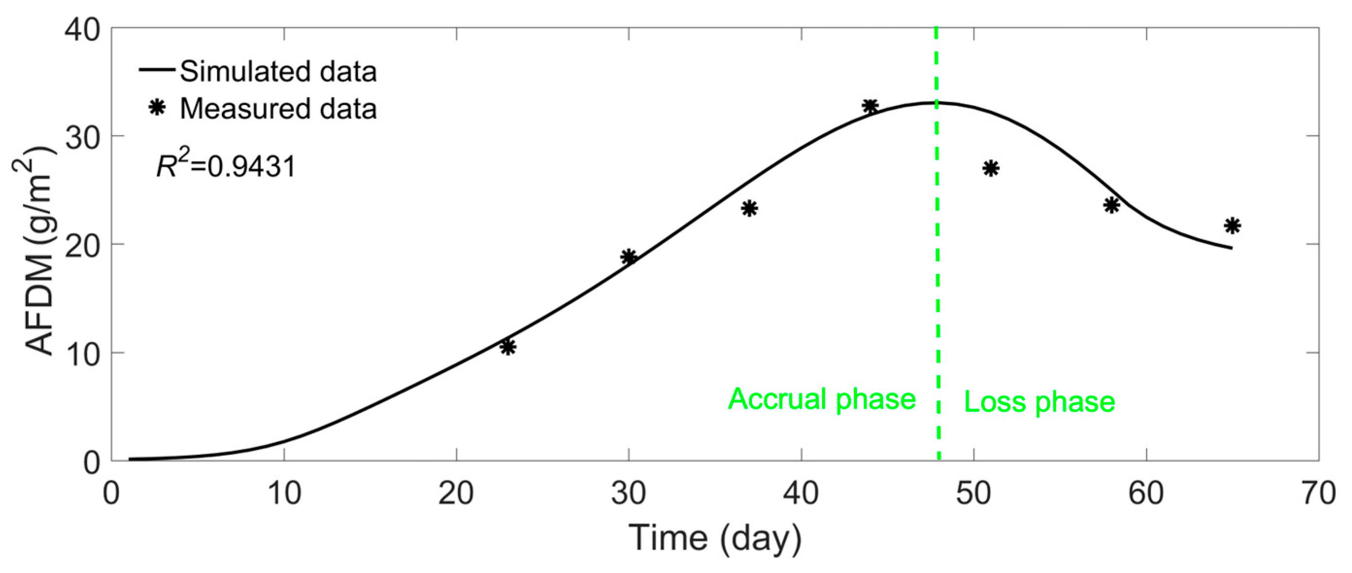
Model Validation and Applicability: Validation against laboratory flume data (65-day biofilm growth cycle) demonstrated the model’s accuracy in simulating biomass trends (ash-free dry mass) and velocity distribution patterns, confirming its reliability under short-term, homogeneous substrate conditions.
(3)
Theoretical Innovation and Engineering Value: By establishing a dynamic correlation model between biofilm thickness and roughness parameters, this study addresses the limitations of conventional models that neglect biofilm–flow coupling effects. It provides a numerical platform for optimizing ecological river restoration strategies, such as balancing pollutant removal efficiency with hydraulic resistance.

Author Contributions

Conceptualization, Y.B.; methodology, H.W.; software, M.W.; validation, Y.B.; formal analysis, M.W.; investigation, H.W.; resources, H.W.; data curation, M.W.; writing—original draft preparation, Y.B.; writing—review and editing, Y.B.; All authors have read and agreed to the published version of the manuscript.

Funding

This study has been funded by Nanxun scholars program of ZJWEU (RC2023010952).

Institutional Review Board Statement

Not applicable.

Informed Consent Statement

Not applicable.

Data Availability Statement

The original contributions presented in this study are included in the article. Further inquiries can be directed to the corresponding author.

Acknowledgments

Nanxun scholars program of ZJWEU (RC2023010952).

Conflicts of Interest

The authors declare no conflict of interest.

References

  1. Zhao, J.; Rao, M.; Zhang, H.; Wang, Q.; Shen, Y.; Ye, J.; Zhang, S. Evolution of Interspecific Interactions Underlying the Nonlinear Relationship Between Active Biomass and Pollutant Degradation Capacity in Bioelectrochemical Systems. Water Res. 2025, 274, 123071. [Google Scholar] [CrossRef] [PubMed]
  2. Anlanger, C.; Risse-Buhl, U.; von Schiller, D.; Noss, C.; Weitere, M.; Lorke, A. Hydraulic and Biological Controls of Biofilm Nitrogen Uptake in Gravel-Bed Streams. Limnol. Oceanogr. 2021, 66, 3887–3900. [Google Scholar] [CrossRef]
  3. Zhang, L.; Luo, W. Reach-Averaged Flow Resistance in Gravel-Bed Streams. J. Water Clim. Chang. 2021, 12, 1580–1597. [Google Scholar] [CrossRef]
  4. Nikora, V.; Goring, D.; McEwan, I.; Griffiths, G. Spatially Averaged Open-Channel Flow over Rough Bed. J. Hydraul. Eng. 2001, 127, 123–133. [Google Scholar] [CrossRef]
  5. Afzalimehr, H.; Maddahi, M.R.; Sui, J. Bedform Characteristics in a Gravel-Bed River. J. Hydrol. Hydromech. 2017, 65, 366. [Google Scholar] [CrossRef]
  6. Bertin, S.; Groom, J.; Friedrich, H. Isolating Roughness Scales of Gravel-Bed Patches. Water Resour. Res. 2017, 53, 6841–6856. [Google Scholar] [CrossRef]
  7. Dey, S. Fluvial Hydrodynamics: Hydrodynamic and Sediment Transport Phenomena; Springer: Berlin, Germany, 2014. [Google Scholar]
  8. Hardy, R.J.; Best, J.L.; Lane, S.N.; Carbonneau, P.E. Coherent Flow Structures in a Depth-Limited Flow over a Gravel Surface: The Role of Near-Bed Turbulence and Influence of Reynolds Number. J. Geophys. Res. Earth Surf. 2009, 114, F01003. [Google Scholar] [CrossRef]
  9. van der Mark, C.F.; Blom, A.; Hulscher, S.J.M.H. Quantification of Variability in Bedform Geometry. J. Geophys. Res. Earth Surf. 2008, 113, F03020. [Google Scholar] [CrossRef]
  10. Dreszer, C.; Vrouwenvelder, J.S.; Paulitsch-Fuchs, A.H.; Zwijnenburg, A.; Kruithof, J.C.; Flemming, H.C. Hydraulic Resistance of Biofilms. J. Membr. Sci. 2013, 429, 436–447. [Google Scholar] [CrossRef]
  11. Battin, T.J.; Kaplan, L.A.; Newbold, J.D.; Cheng, X.; Hansen, C. Effects of Current Velocity on the Nascent Architecture of Stream Microbial Biofilms. Appl. Environ. Microbiol. 2003, 69, 5443–5452. [Google Scholar] [CrossRef]
  12. Bilgili, E.; Bomers, A.; van Lente, G.J.W.; Huthoff, F.; Hulscher, S.J. The Effect of a Local Mesh Refinement on Hydraulic Modelling of River Meanders. River Res. Appl. 2023, 39, 832–846. [Google Scholar] [CrossRef]
  13. Grimaldi, S.; Li, Y.; Walker, J.P.; Pauwels, V.R.N. Effective Representation of River Geometry in Hydraulic Flood Forecast Models. Water Resour. Res. 2018, 54, 1031–1057. [Google Scholar] [CrossRef]
  14. Nagata, N.; Hosoda, T.; Nakato, T.; Muramoto, Y. Three-Dimensional Numerical Model for Flow and Bed Deformation around River Hydraulic Structures. J. Hydraul. Eng. 2005, 131, 1074–1087. [Google Scholar] [CrossRef]
  15. Ahn, J.; Na, Y.; Park, S.W. Development of Two-Dimensional Inundation Modelling Process Using MIKE21 Model. KSCE J. Civ. Eng. 2019, 23, 3968–3977. [Google Scholar] [CrossRef]
  16. Xu, C.; Tian, J.; Liu, Z.; Wang, R.; Wang, G. Three-Dimensional Reverse Modeling and Hydraulic Analysis of the Intake Structure of Pumping Stations on Sediment-Laden Rivers. Water Res. Manag. 2023, 37, 537–555. [Google Scholar] [CrossRef]
  17. Tassi, P.; Benson, T.; Delinares, M.; Fontaine, J.; Huybrechts, N.; Kopmann, R.; Walther, R. GAIA—A Unified Framework for Sediment Transport and Bed Evolution in Rivers, Coastal Seas and Transitional Waters in the TELEMAC-MASCARET Modelling System. Environ. Model. Softw. 2023, 159, 105544. [Google Scholar] [CrossRef]
  18. Darijani, Z.; Ghaeini-Hessaroeyeh, M.; Fadaei-Kermani, E. Flood Inundation and Hazard Mapping Using the HEC-RAS 2D Model: A Case Study of Adoori River, Iran. Model. Earth Syst. Environ. 2025, 11, 78. [Google Scholar] [CrossRef]
  19. Haddach, A.; Smaoui, H.; Radi, B. The Study of Coastal Flows Based on Lattice Boltzmann Method: Application Oualidia Lagoon. J. Braz. Soc. Mech. Sci. Eng. 2024, 46, 225. [Google Scholar] [CrossRef]
  20. Biscarini, C.; Di Francesco, S.; Mencattini, M. Application of the Lattice Boltzmann Method for Large-Scale Hydraulic Problems. Int. J. Numer. Methods Heat Fluid Flow 2011, 21, 584–601. [Google Scholar] [CrossRef]
  21. Delavar, M.A.; Wang, J. Lattice Boltzmann Method in Modeling Biofilm Formation, Growth and Detachment. Sustainability 2021, 13, 7968. [Google Scholar] [CrossRef]
  22. Bray, D.I. Estimating Average Velocity in Gravel-Bed Rivers. J. Hydraul. Div. 1979, 105, 1103–1122. [Google Scholar] [CrossRef]
  23. Huai, W.; Hu, Y.; Zeng, Y.; Han, J. Velocity Distribution for Open Channel Flows with Suspended Vegetation. Adv. Water Resour. 2012, 49, 56–61. [Google Scholar] [CrossRef]
  24. Wu, F.C.; Shen, H.W.; Chou, Y.J. Variation of Roughness Coefficients for Unsubmerged and Submerged Vegetation. J. Hydraul. Eng. 1999, 125, 934–942. [Google Scholar] [CrossRef]
  25. Ding, Y.; Liu, H.; Peng, Y.; Xing, L. Lattice Boltzmann Method for Rain-Induced Overland Flow. J. Hydrol. 2018, 562, 789–795. [Google Scholar] [CrossRef]
  26. Zhao, F.; Huai, W.; Li, D. Numerical Modeling of Open Channel Flow with Suspended Canopy. Adv. Water Resour. 2017, 105, 132–143. [Google Scholar] [CrossRef]
  27. Ilseven, E.; Mendoza, M. Lattice Boltzmann Model for Numerical Relativity. Phys. Rev. E 2016, 93, 023303. [Google Scholar] [CrossRef]
  28. Liu, H.; Zhou, J.G.; Burrows, R. Lattice Boltzmann Simulations of the Transient Shallow Water Flows. Adv. Water Resour. 2010, 33, 387–396. [Google Scholar] [CrossRef]
  29. Enouy, R.W.; Walton, K.M.; Malton, I.I. A Mechanistic Derivation of the Monod Bioreaction Equation for a Limiting Nutrient. J. Math. Biol. 2022, 84, 62. [Google Scholar] [CrossRef]
  30. Graba, M.; Moulin, F.Y.; Boulêtreau, S.; Garabétian, F.; Kettab, A.; Eiff, O.; Sauvage, S. Effect of Near-Bed Turbulence on Chronic Detachment of Epilithic Biofilm: Experimental and Modeling Approaches. Water Resour. Res. 2010, 46, W11531. [Google Scholar] [CrossRef]
  31. Uehlinger, U.R.S.; Bührer, H.; Reichert, P. Periphyton Dynamics in a Floodprone Prealpine River: Evaluation of Significant Processes by Modelling. Freshwater Biol. 1996, 36, 249–263. [Google Scholar] [CrossRef]
  32. Fothi, A. Effets Induits de la Turbulence Benthique sur les Mécanismes de Croissance du Périphyton. Ph.D. Dissertation, Toulouse INPT, Toulouse, France, 2002. [Google Scholar]
  33. Labiod, C.; Godillot, R.; Caussade, B. The Relationship Between Stream Periphyton Dynamics and Near-Bed Turbulence in Rough Open-Channel Flow. Ecol. Model. 2007, 209, 78–96. [Google Scholar] [CrossRef]
  34. Marquis, G.A.; Roy, A.G. Effect of Flow Depth and Velocity on the Scales of Macroturbulent Structures in Gravel-Bed Rivers. Geophys. Res. Lett. 2006, 33, L24406. [Google Scholar] [CrossRef]
  35. Milan, D.J. Virtual Velocity of Tracers in a Gravel-Bed River Using Size-Based Competence Duration. Geomorphology 2013, 198, 107–114. [Google Scholar] [CrossRef]
  36. Brenna, A.; Surian, N.; Mao, L. Virtual Velocity Approach for Estimating Bed Material Transport in Gravel-Bed Rivers: Key Factors and Significance. Water Resour. Res. 2019, 55, 1651–1674. [Google Scholar] [CrossRef]
  37. Franca, M.J.; Ferreira, R.M.; Lemmin, U. Parameterization of the Logarithmic Layer of Double-Averaged Streamwise Velocity Profiles in Gravel-Bed River Flows. Adv. Water Resour. 2008, 31, 915–925. [Google Scholar] [CrossRef]
  38. Luo, M.; Ye, C.; Wang, X.; Huang, E.; Yan, X. Analytical Model of Flow Velocity in Gravel-Bed Streams under the Effect of Gravel Array with Different Densities. J. Hydrol. 2022, 608, 127581. [Google Scholar] [CrossRef]
  39. Meier, C.I.; Reid, B.L.; Sandoval, O. Effects of the Invasive Plant Lupinus polyphyllus on Vertical Accretion of Fine Sediment and Nutrient Availability in Bars of the Gravel-Bed Paloma River. Limnologica 2013, 43, 381–387. [Google Scholar] [CrossRef]
  40. Taube, N.; Ryan, M.C.; He, J.; Valeo, C. Phosphorus and Nitrogen Storage, Partitioning, and Export in a Large Gravel Bed River. Sci. Total Environ. 2019, 657, 717–730. [Google Scholar] [CrossRef]
  41. Quinn, J.M.; Rutherford, J.C.; Schiff, S.J. Nutrient Attenuation in a Shallow, Gravel-Bed River. I. In-Situ Chamber Experiments. N. Z. J. Mar. Freshwater Res. 2020, 54, 393–409. [Google Scholar] [CrossRef]
  42. Tsuchiya, Y.; Eda, S.; Kiriyama, C.; Asada, T.; Morisaki, H. Analysis of Dissolved Organic Nutrients in the Interstitial Water of Natural Biofilms. Microb. Ecol. 2016, 72, 85–95. [Google Scholar] [CrossRef]
  43. Paudel, S.; Singh, U.; Crosato, A.; Franca, M.J. Effects of Initial and Boundary Conditions on Gravel-Bed River Morphology. Adv. Water Resour. 2022, 166, 104256. [Google Scholar] [CrossRef]
Figure 1. Temporal dynamics of biofilm growth cycles on gravel-bed slopes: (a) 7 days after inoculum, (b) 14 days after inoculum, (c) 30 days after inoculum.
Sustainability 17 04905 g001
Figure 2. The width of gravel and biofilm.
Sustainability 17 04905 g002
Figure 3. Distribution functions at the boundaries.
Sustainability 17 04905 g003
Figure 4. The flowchart of the numerical model.
Sustainability 17 04905 g004
Figure 5. The structure of the experimental flume.
Sustainability 17 04905 g005
Figure 6. The simulated result of AFDM.
Sustainability 17 04905 g006
Figure 7. The simulated result of velocity ((a) presents vertical velocity distribution at 16 days, (b) presents vertical velocity distribution at 33 days, (c) presents vertical velocity distribution at 38 days, (d) presents vertical velocity distribution at 61 days).
Sustainability 17 04905 g007
Table 1. Parameters of Equation (15).
ParametersValueAccording toReferences
μ m a x 1.1 d−1Refer to the typical range of laboratory and field research (0.5–1.2 d−1), and optimize experimental data through model fitting.Uehlinger et al. [31]
k i n v 0.085 g−1·m2The self-inhibitory effect of biomass on growth rate was determined by fitting experimental data using the least squares method.Graba et al. [30]
C d e t 0.0014 d−1The effectiveness of using roughness Reynolds number as a driving factor for separation was verified through calibration of its correlation with the separation process.Fothi [32]; Labiod et al. [33]
Disclaimer/Publisher’s Note: The statements, opinions and data contained in all publications are solely those of the individual author(s) and contributor(s) and not of MDPI and/or the editor(s). MDPI and/or the editor(s) disclaim responsibility for any injury to people or property resulting from any ideas, methods, instructions or products referred to in the content.

