Optimization of Calibration Settings for Passive Anti-Islanding Protections Using a Bayesian Entropy Methodology to Support the Sustainable Integration of Renewable Distributed Generation

Abstract

The global pursuit of sustainable development increasingly depends on integrating renewable energy sources into power systems, with distributed generation (DG) playing a vital role. However, this integration presents technical challenges, particularly the risk of unintentional islanding. Anti-islanding protections are essential for detecting and isolating such events, as required by IEEE 1547, within two seconds. Yet, calibrating these protections to balance sensitivity and reliability remains a complex task, as evidenced by incidents like the UK power outage on 9 August 2019 and the Southwestern Utah event on 10 April 2023. This study introduces the Bayesian Entropy Methodology (BEM), an innovative approach that employs entropy as a model for uncertainty in protection decision-making. By leveraging Bayesian inference, BEM identifies optimal calibration settings for time delay and pick-up thresholds, minimizing uncertainty and effectively balancing sensitivity and reliability. The methodology incorporates a modified entropy surface to enhance optimization outcomes. Applied to the IEEE 34-node test system, BEM demonstrates the ability to determine optimal settings with a significantly reduced training dataset, leading to substantial computational savings. By enhancing the reliability of anti-islanding protections, BEM facilitates the secure integration of renewable DG, contributing to the sustainable development of modern power systems.

1. Introduction

The transition to a more sustainable, resilient, and decarbonized energy system is accelerating the deployment of distributed generation (DG), mainly from renewable sources. However, integrating DG into distribution networks introduces several technical challenges, including the risk of unintentional islanding [1]. These islands occur when a radial distribution grid, which is not prepared for islanded operation, loses its connection with the main grid but remains energized by the downstream connected DG units [2]. The island’s electrical variables become uncontrollable, which constitutes a risk to the safety of users and maintenance personnel [3,4]. To prevent this problem, each DG must have special protection to identify islanding and disconnect itself. This protection is called anti-islanding (also known as loss of main) and is mandatory in many regulations and grid codes [4,5,6,7,8,9].

A critical characteristic of anti-islanding protection is sensitivity, defined as its ability to detect the formation of an island [10] rapidly. Another essential characteristic of anti-islanding protection is its reliability, defined as the ability not to trigger false alarms under various disturbances [10]. These disturbances, to which the anti-islanding protection must demonstrate reliable behavior, include both distribution system disturbances and bulk power system (BPS) disturbances, which the protection should not mistakenly identify as islanding events.

In a context of high DG penetration, the unreliable behavior of anti-islanding protection following a power system disturbance can trigger a massive disconnection of DG if the anti-islanding protections mistakenly interpret this event as an islanding event. This is precisely what caused the Low Frequency Demand Disconnection (LFDD) on 9 August 2019, following a disturbance in the UK bulk power system, which began with a lightning strike and was followed by other events in the system [11].

Similarly, on 10 April 2023, a significant disturbance in the Southwestern United States highlighted ongoing challenges with anti-islanding protection in large-scale solar photovoltaic (PV) installations. During this event, one solar PV plant in Utah incorrectly triggered its anti-islanding protections in response to a usually cleared fault in the bulk power system (BPS). This led to the disconnection of over 900 MW of generation, as the anti-islanding protections misinterpreted the transient grid disturbance as an islanding event. Despite being intended for distribution-level applications, these protections were not adequately adjusted for BPS-connected inverters, further emphasizing the need for enhanced coordination and configuration of protection schemes in high-penetration DG scenarios [12]. This incident, alongside the 2019 UK event, underscores the systemic risk that unreliable anti-islanding behavior poses to grid stability in systems with substantial DG.

The literature presents various methodologies for island detection, including remote methods, based on communications, and local methods, which are classified as active or passive depending on whether a disturbance is actively introduced into the network [13,14]. Among these, passive local methods are particularly significant, as they can be applied across a broader range of generation technologies, whereas active methods are typically limited to converter-based generation. This work, however, focuses on passive methods.

Passive islanding detection methods are generally divided into traditional and advanced categories. Conventional methods include the frequency and voltage threshold approach (FVT) identified by ANSI 81U/O and ANSI 27/59, the rate of change of frequency (RoCoF) approach as per ANSI 81R [15], and the voltage vector shift (VVS) detection approach [16,17,18]. These are among the most widely employed techniques in distribution systems with significant DER penetration [7,19,20].

The primary challenge associated with classical passive anti-islanding protections lies in their large non-detection zones (NDZs). These NDZs represent operational conditions where the electrical variables, such as voltage, frequency, or RoCoF, remain within acceptable limits despite the formation of an island, making detection difficult. This issue arises because passive methods rely on thresholds to trigger detection. With minimal mismatch between generation and load, the system remains stable within those thresholds, leading to undetected islanding conditions [21,22,23,24].

Concerning the current regulations, the IEEE 1547-2018 standard [5] establishes ride-through requirements, specifying the voltage, frequency, and RoCoF ranges within which DG must remain connected to the grid during adverse events. However, these requirements necessitate the adjustment of passive anti-islanding protections with calibration thresholds that increase the NDZs, thereby reducing their effectiveness in detecting specific critical islanding scenarios.

Advanced passive methods, in contrast, employ advanced signal processing, machine learning, and classification techniques to enhance their performance and reduce false tripping. However, despite their advantages, these methods require devices with high processing capabilities and significant computational resources for implementation due to the extensive data sets needed for training [25,26,27]. Like traditional methods, advanced approaches still depend on accurately defining operational thresholds, which remains challenging for passive detection methods [28].

In [29], the Automatic Setting Map Methodology (ASMM) is presented. It proposes calculating optimal settings through an algorithm that maximizes a weighted objective function, where weights can be arbitrarily chosen based on a preference for higher sensitivity or stability. Significant computational effort is required due to the number of cases employed to maximize the objective function. Moreover, the methodology has not been evaluated for frequency transients caused by disturbances in the EPS, whose duration can be longer than the times involved in islanding detection, complicating the application of this method, which is based on the superposition of the variables’ dynamics in a temporal framework. Additionally, as it is based on a dynamic analysis of the variables, applying this method for the threshold adjustment of other protections necessitates modifications to the original algorithm, further increasing the computational effort, as is presented in [30], where the ASMM is used to find the best under-voltage block setting to improve the performance of commonly used passive IDM.

In [31], a methodology based on dynamic security regions has been presented to identify the minimum requirements for RoCoF-based (ANSI 81R) anti-islanding protections for DERs, which ensure the safe operation of the Brazilian Interconnected Power System. While this methodology successfully identified minimal safety conditions for setting the lowest RoCoF thresholds, it did not provide an analysis of the performance of these settings in terms of sensitivity across various islanding scenarios, relegating the contribution of this work solely to the study of security in the EPS.

The Bayesian Entropy Methodology (BEM) offers a novel approach for optimizing anti-islanding protection settings, balancing sensitivity and reliability. BEM minimizes the uncertainty in protection decisions by using entropy to measure uncertainty in detecting islanding events. Employing Bayesian inference and entropy modeling determines the optimal calibration thresholds (such as time delay and pickup settings) that enhance stability and reliability while reducing NDZs. The advantage of BEM lies in its ability to achieve these settings without the need for extensive computational resources or large datasets, as seen in other works to optimize the settings for anti-islanding protection [32].

This work presents an improvement to the BEM by introducing a modification in the entropy modeling, incorporating specific penalties to eliminate low-entropy zones with no practical application in protection systems. This modification enhances the original BEM. Additionally, the modified entropy within BEM has been applied to obtain the optimal adjustment settings for passive protections in the IEEE 34-node test system. The results indicate that BEM allows for identifying optimal settings for passive protections in response to a wide range of events, including BPS disturbances, while utilizing reduced datasets. This highlights one of the main contributions of BEM: significantly reducing the computational effort required to achieve optimal anti-islanding protection settings for passive systems.

The remainder of this work is organized as follows: Section 2 presents the BEM and proposed modifications in the entropy modeling through the modified entropy function. Section 3 introduces the IEEE 34-node test system and its changes, including the connection to a three-bus BPS to generate disturbance cases in this power system. Also, the datasets of cases obtained from this test system are presented. Section 4 presents the results obtained and the validation instances. And finally, in Section 5, the conclusions are presented.

2. Modified Entropy Surface and Bayesian Entropy Methodology

The BEM treats an anti-islanding protection system as a black box that processes information from the Point of Common Coupling (PCC) and decides whether to disconnect the Distributed Generator (DG) during a disturbance. The simplified protection model shown in Figure 1 assumes that the ability to detect islanding events primarily depends on the calibration of the protection system, specifically the time-delay ($td$) and pick-up ($pk$) settings. Thus, for each event that occurs (whether a disturbance or an islanding case), the protection system will have a certain probability of correctly detecting the event based on these settings. For islanding events, the probability of correctly detecting the island is denoted as $p_{D/I}(td,pk)$, which represents the probability of detection given that an island has occurred. Similarly, for non-islanding events, $p_{ND/NI}(td,pk)$ represents the probability of not incorrectly detecting an island when no islanding event has occurred.

The calibration parameters, $td$ and $pk$ for the simplified protection model presented in Figure 1 define its overall behavior. An ideal protection system would have probabilities $p_{D/I}$ and $p_{ND/NI}$ equal to one, meaning perfect detection of islanding events and perfect avoidance of false positives. On the other hand, a chaotic protection system, where decisions are predominantly random, would have these probabilities close to 0.5, indicating erratic and unpredictable behavior, which is precisely the opposite of what is desired in a protection system. The objective of BEM is to assign a specific calibration value ($td$ and pick-up: $pk$ settings), corresponding to a specific entropy value. In this model, entropy serves as a measure of the uncertainty or chaos in the decisions made by the anti-islanding protection system.

Equation (1) presents the entropy of a set of probabilities. In this context, entropy quantifies the uncertainty associated with protection actions—whether the protection system correctly detects an islanding event or mistakenly identifies a disturbance as an island.

$$H_{protection}=\sum _{i=1}^{i=N}{p}_i\mathit{log}{\displaystyle \frac{1}{p_i}}$$

(1)

In Equation (1), the total entropy (entropy of the protection) is obtained by the weighted sum of the information from the probability associated with each event defined for the operation of the electrical protection, according to the defined probabilistic tree model [32]. Using these probabilities, presented in Equation (2), the protection entropy is calculated by treating it as a source of messages (trip or no trip) based on Shannon’s definition of entropy [33].

$$p_i\in \left\{p_{D/I},p_{ND/I},p_{D/NI},p_{ND/NI},p_{I/T},p_{NI/T},p_{I/NT},p_{NI/NT}\right\}$$

(2)

In Equation (2), the set of forward and backward success and failure probabilities is presented [32]. The subscripts stand for D (detect), I (islanding), NI (no-islanding), T (trip), and NT (no-trip). Each probability in this set represents a specific outcome:

• $p_{D/I}$ is the probability of detecting an island when it has actually occurred (forward success).
• $p_{D/NI}$ is the probability of mistakenly identifying a disturbance as an island (forward failure).
• $p_{ND/I}$ is the probability of failing to detect an island when it has occurred (forward failure).
• $p_{ND/NI}$ is the probability of correctly identifying a disturbance without mistaking it for an island (forward success).
• $p_{I/T}$ represents the probability that, given the protection was triggered, the cause was an actual islanding event (backward success).
• $p_{NI/T}$ is the probability that, given the protection was triggered, the cause was a disturbance (backward failure).
• $p_{I/NT}$ is the probability that, given the protection did not trigger, an islanding event still occurred (backward failure).
• $p_{NI/NT}$ is the probability that, given the protection did not trigger, the event was indeed a disturbance and not an island (backward success).

From the set of probabilities presented in Equation (2), the independent variables are $p_{D/I}$ and $p_{ND/NI}$, as the remaining probabilities can be derived from these two [32]. Therefore, by estimating these two probabilities, it is possible to calculate the protection entropy using Shannon’s entropy formula, as shown in Equation (1).

The entropy model in Equation (1) reaches its maximum (maximum uncertainty) when all the probabilities defined in Equation (2) are equal $(p_i=0.5)$, and it is zero when the probabilities $p_{D/I}$ and $p_{ND/NI}$ are equal to one, representing an ideally perfect protection that always detects islanding events with no NDZ and never trips erroneously. However, this entropy model also results in zero under certain mathematical conditions that make no practical sense. When both probabilities, $p_{D/I}$ and $p_{ND/NI}$, approach zero, the entropy model in Equation (1) also tends to zero, representing an ideal protection that never trips under any circumstances. In this hypothetical case, there is no uncertainty, but it leads to an unrealistic scenario for modeling electrical protection [32].

To address this issue in the original uncertainty model of Equation (1) [33], this work introduces a more practical model, fitted to the search for minimum entropy in electrical protection systems. This improved model, defined as modified entropy (C), and is presented in Equation (3).

$$C_{protection}=\mathit{log}\left[ k^{-(p_{D/I}-a)}\left({\displaystyle \frac{1}{p_{D/I}}}-1\right)+k^{-(p_{ND/NI}-a)}\left({\displaystyle \frac{1}{p_{ND/NI}}}-1\right)+\prod _{i=1}^{i=N}{\displaystyle \frac{1}{p_i^{p_i}}} \right]$$

(3)

The modification of the model proposed in Equation (3) includes two terms that act as penalties when both probabilities $p_{D/I}$ and $p_{ND/NI}$ approach zero. These penalties can be adjusted using the constants $k$ and $a$, which allow fine-tuning the modified entropy model (C) relative to the original entropy model (H). In this way, it is possible to obtain an entropy model that penalizes calibrations that lead to protection having probabilities $p_{D/I}$ and $p_{ND/NI}$ close to zero and that adjusts as closely as possible to the original Shannon entropy model, allowing fine-tuning through the parameters k, y, and a defined in Equation (3). The values of a and k control how “quickly” the C surface converges to the H surface as the probabilities approach unity. 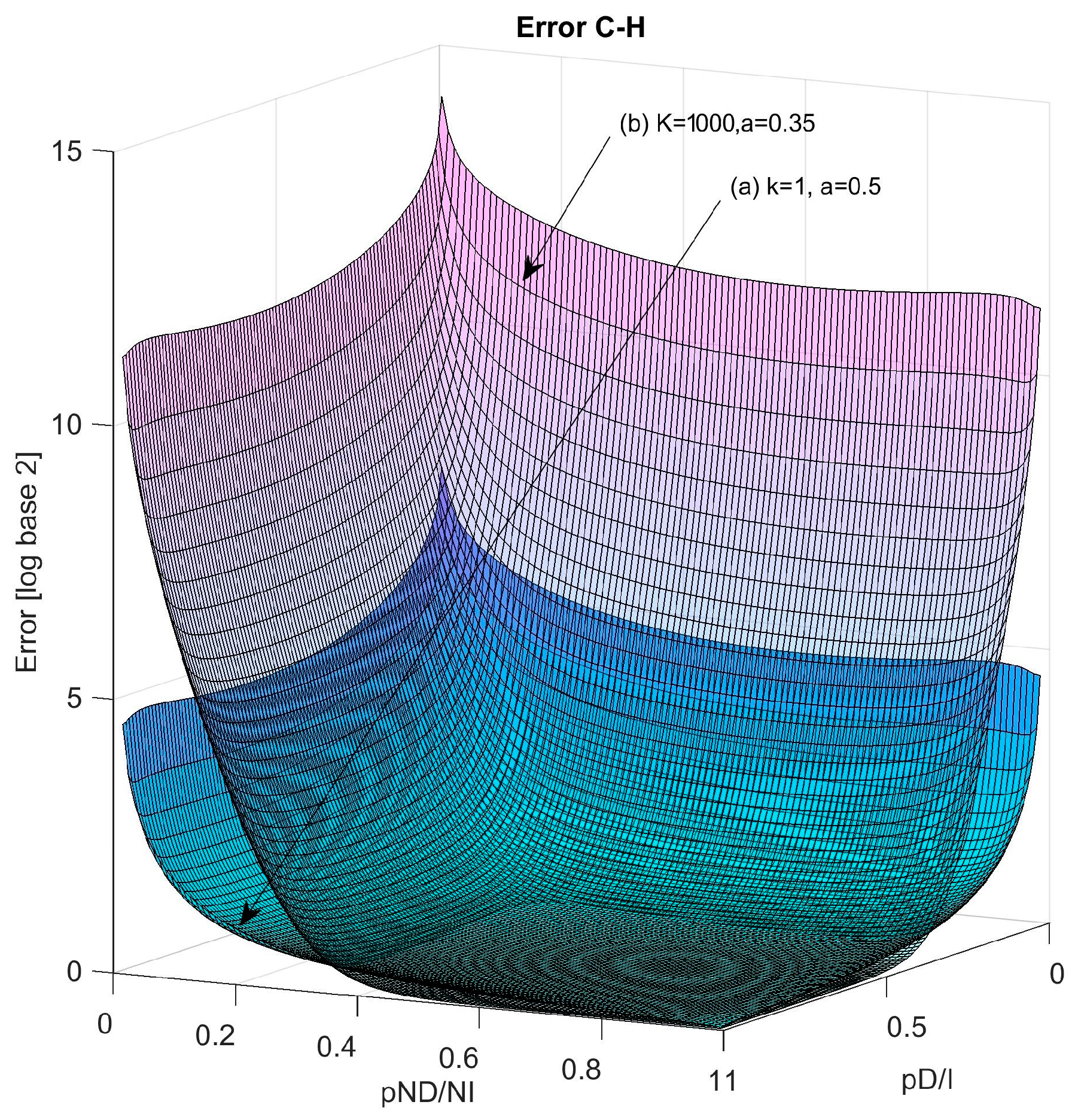The adjustment of these parameters was carried out through trial and error, determining the most appropriate values as shown in Figure 2. These parameters introduce degrees of freedom that allow for fine-tuning, optimizing the application of the proposed methodology.

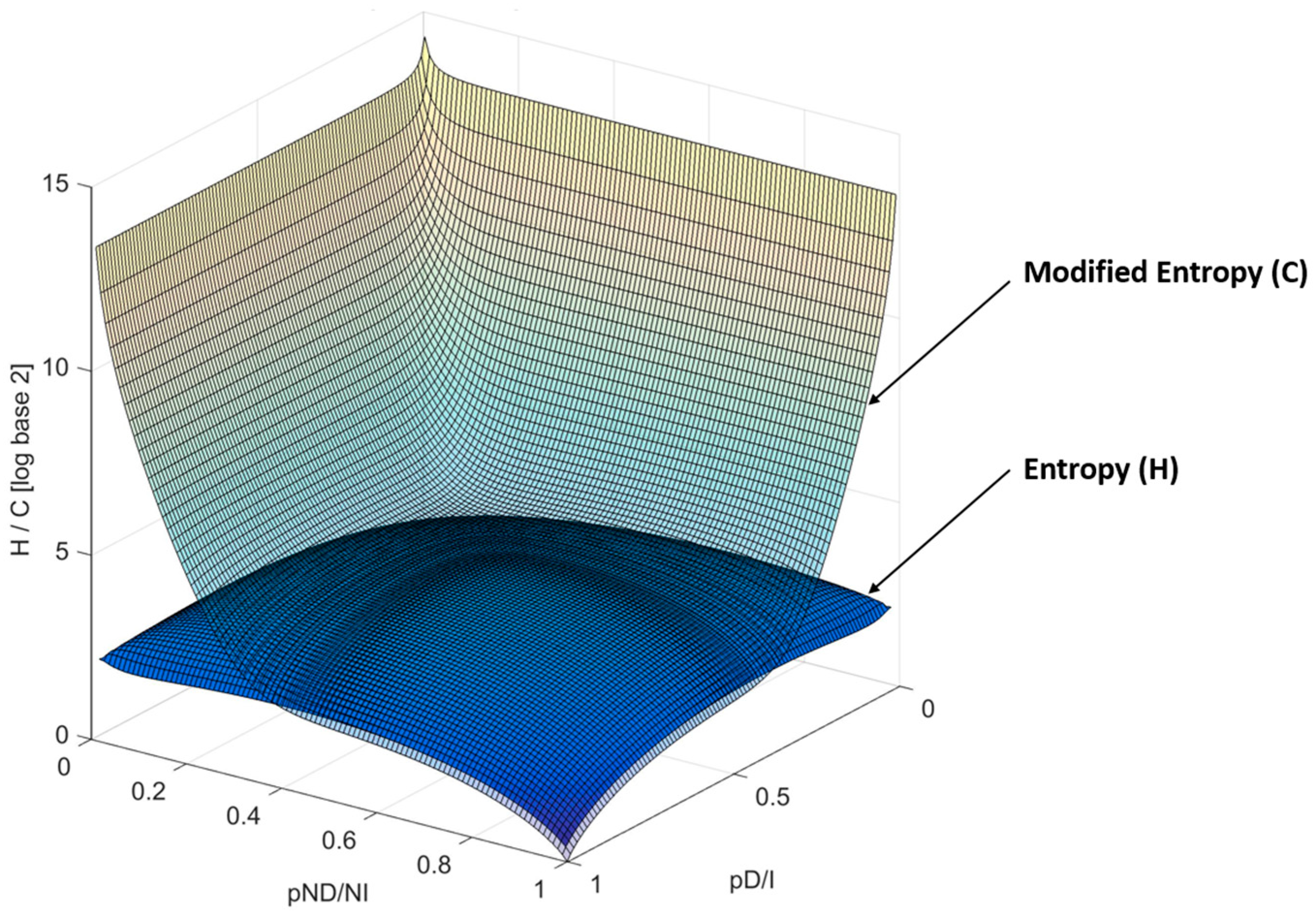
Figure 3 presents a comparison of entropy surfaces (H) and modified entropy (C). Figure 2 shows error surfaces for different values of the adjustment parameters k, y, and a.

The application of the entropy surface (H) described in Equation (1) is not suitable as a direct objective function due to the presence of mathematical minima that lack practical relevance in protection systems. In contrast, the modified entropy surface (C) serves as a cost function that facilitates the search for minimum uncertainty in the protection system, and allows for simultaneous modeling of the uncertainty or chaos within the protection system. Furthermore, near the global minimum, this modified surface enables direct calculation of entropy, converging almost without error to the Shannon entropy model.

To estimate the probabilities $p_{D/I}$ and $p_{ND/NI}$, the BEM defines a statistical experiment by modeling islanding detection as a Bernoulli trial. This experiment uses Bayesian inference, which efficiently computes these probabilities based on a limited dataset, reducing the computational burden. Figure 4 presents the flowchart for the application of the BEM.

Through the Bayesian approach, the probabilities of success are calculated as presented in Equation (4):

$${\theta }_j^{\ast }={\displaystyle \frac{m\overline{x}+1}{m·n_j+2}}$$

(4)

Equation (4) is the Bayes estimate of the parameter ${\theta }_j$ under the squared-error loss function, $\overline{x}$ is the average number of successful cases, $m$ is the number of times the statistical island detection experiment is repeated (in three-phase systems, $m=3$), and $n_j$ is the number of cases analyzed in the defined dataset. In the specific problem of estimating the probabilities of anti-islanding protection ${\theta }_{j=1}=p_{D/I}$ and ${\theta }_{j=2}=p_{ND/NI}$. This result allows for the point estimation of forward population success probabilities based on fixed anti-islanding settings, $td$ and $pk$ [32].

To carry out probability estimation using Bayesian inference, it is necessary to define a statistical experiment in which a dataset of island events of $n_i$ cases and non-island events of $n_{ni}$ cases are, respectively, defined. These events must be randomly selected from a test system. Defining the size of the datasets allows for determining the minimum achievable entropy, as seen in Equations (5) and (6), which is one of the main contributions of the BEM, as the minimum achievable entropy precisely defines the required size of these case sets [32].

$$\left\{\begin{array}{c}{p_{D/I}^{\ast }}_{MAX} ={\displaystyle \frac{{m·n}_i+1}{{m·n}_i+2}}\\ {p_{ND/NI}^{\ast }}_{MAX}={\displaystyle \frac{{m·n}_{ni}+1}{{m·n}_{ni}+2}}\end{array}\right.$$

(5)

$$H({p_{D/I}^{\ast }}_{MAX}, {p_{ND/NI}^{\ast }}_{MAX})=H_{min}$$

(6)

In Equations (5) and (6), ${p_{D/I}^{\ast }}_{MAX}$ and ${p_{ND/NI}^{\ast }}_{MAX}$ represent the maximum probability values that can be estimated through the definition of a given experiment (defined by the $n_j$ island and non-island events randomly selected). This experiment also determines the minimum possible entropy, $H_{min}$. To achieve lower entropy values, the size of the datasets must be increased. In this way, the necessary dataset size can be precisely determined to obtain a desired entropy value using the BEM.

It is important to highlight that, according to the statistical experiment and Bayesian inference approach defined in this study, the minimum achievable entropy shown in Equation (6) depends exclusively on the size of the dataset. As such, it is scalable to any test power system size, given the assumption that islanding and non-islanding cases are randomly sampled from a universe of infinite possible events. These cases could even correspond to real operating conditions from an actual power system or a combination of real and simulated events.

The size of the power system does not matter—both the minimum achievable entropy and the maximum probabilities depend solely on the size of the dataset and are related through Equations (5) and (6).

If 30 islanding cases and 30 non-islanding events are selected, a dataset of only 60 cases is formed. This results in maximum probabilities of ${p_{D/I}^{\ast }}_{MAX}={p_{ND/NI}^{\ast }}_{MAX}=0.98913$. This maximum probability is interpreted as the highest probability that the BEM can “observe”. In other words, even if a theoretically perfect protection system is tested—one with probabilities of success equal to one—the BEM would only be able to estimate its performance using these maximum probabilities, as described in Equation (5).

In this sense, Equation (5), which relates the maximum observable probabilities to the size of the dataset, defines the limit of uncertainty that can be “seen” under a given experiment, determined by the dataset size. This is a key result, as it allows for accurately determining the dataset size required to achieve a desired level of performance. In the example of the ideal protection system, the gap between a perfect probability (equal to one) and the maximum probability estimated by the BEM represents the residual uncertainty intrinsic to the experiment itself.

3. Modified IEEE 34-Node Test System and Dataset Generation

3.1. Modified IEEE 34-Node Test System

The modified IEEE 34-node test system was utilized in this study to apply the BEM. The IEEE 34-node system [34] is widely used in research due to its unbalanced characteristics and its suitability for validating protection schemes in distribution networks with DG [29,34,35,36,37]. Figure 5 presents the single-line diagram of the model with the implemented modifications. An additional low-voltage node, designated as Node 848-B, was added to the original model, where two distributed generation units of different types were incorporated. DG1 is a synchronous generator, while DG2 is a converter-based unit. Each of these units represents parallel machines/converters. By varying the number of parallel units, different islanding generation scenarios can be simulated during the conducted tests. The system was modeled using DIgSILENT Power Factory 2018 SP3. Appendix A presents some parameters omitted in this section of the employed system model.

Figure 5 shows the location of possible faults considered and different islanding scenarios for the Distributed Generators connected at Node 848-B. In each of these scenarios, the island’s load varies by including more or fewer loads defined initially in the test system, specifically, those from nodes 842 to 848 and the lines.

Additionally, a simplified three-bus BPS was integrated to simulate disturbances such as frequency transients, as shown in Figure 6. This modification replicates the essential features of a larger-scale power system, operating at 132 kV, enabling studies under realistic conditions. In this BPS, frequency transients can be simulated due to events such as the disconnection of generation units or fault clearance in transmission lines. Furthermore, various renewable generation units were included to simulate different levels of inertia, allowing for more realistic scenarios where disturbances in the BPS could impact anti-islanding protection, testing its ability to avoid false tripping under these conditions.

3.2. Islanding Events Considered at Node 848

To obtain the sets of islanding cases, multiple scenarios were simulated at Node 848. Three scenarios were considered for each combination of distributed generation with mixed technologies, taking into account different percentages of penetration from converter-based generation. Additionally, it was considered that the island topology could vary, meaning that the islands could form due to network disconnection at different points. In all islanding cases, the variables related to demand, topology, and generation scenarios were considered randomly, starting with the demand scenario of the distribution system. The DPL code programmed for the sampling of islanding cases is summarized in the block diagram presented in Figure 7.

The islanding cases at Node 848 were generated by running multiple EMT simulations automatically using an appropriate DPL code in DigSILENT Power Factory. The islands at Node 848 were created by allowing different scenarios with the random opening of 4 lines after 0.25 s of simulation, generating 4 possible island configurations, as shown in Figure 6.

3.2.1. Demand Scenarios in the IEEE 34-Node Test System

The demand generation cases were created using ten scenarios based on the original demands of the IEEE 34-node test system [34]. For each scenario, the demand values for each load in the system were randomly obtained and assigned within specific limits. For example, in Scenario 1, the minimum demand is 0% and the maximum is 10%. In Scenario 2, the minimum demand increases to 10% and the maximum is 20%, and so on, increasing in 10% increments up to Scenario 10, where the minimum demand is 90% and the maximum demand reaches 100%. In all scenarios, the power factor for the minimum demand is 90%, and for the maximum demand, it is 107.5%, consistently applied across the scenarios. This setup allows for a variety of demand conditions, representing different levels of load for system analysis and simulation.

3.2.2. Islanding Scenarios at Node 848 in the IEEE 34-Node Test System

To evaluate different levels of penetration of inverter-based DG and its impact on island detection capability, three generation scenarios were designed, each representing different combinations of synchronous generators and inverters:

The first generation scenario includes three synchronous generators operating in parallel, complemented by a single inverter. This setup focuses on creating a challenge for island detection by involving a higher proportion of synchronous DG with high inertia, which provides more stability to the island.

In the second generation scenario, the configuration consists of two inverters and two synchronous generators. This combination balances synchronous and inverter-based generation, allowing for the examination of the impact of moderate DG penetration on the island’s dynamics and inertia.

The third generation scenario involves three inverters and only one synchronous generator, highlighting the impact of a higher penetration of inverter-based DG, which reduces the inertia in islanding cases (

Table 1. Generation scenarios for island formation at Node 848.

Scenario Gen. Node 848	% SG	% INV	PDG1 [KW]	QDG1 [KVAR]	NDG1	PDG2 [KW]	QDG2 [KVAR]	NDG2
1	75	25	261	150	3	87	50	1
2	50	50	174	100	2	174	100	2
3	25	25	87	50	1	261	150	3

).

Regarding island formation, in this scenario, four potential disconnection points within the system were considered, providing a random basis to vary the topology of the generated island. By disconnecting the lines indicated in

Table 2. Island formation points considered for Node 848.

Island Topology	Island Formation Node	Element to Disconnect	Disconnection Time
1	848	Line 846–848	0.25 s
2	846	Line 844–846	0.25 s
3	844	Line 842–844	0.25 s
4	842	Line 834–842	0.25 s

, it is possible to modify the configuration of the electrical system forming the island, allowing for an evaluation of how different island topologies, demand variation, and the resulting imbalance affect the effectiveness of the anti-islanding protection.

3.3. Disturbance Cases for Node 848

3.3.1. Disturbances in the Distribution System

For the fault cases, 24 possible network elements adjacent to Node 848 were considered as the locations for disturbances, including both lines and nodes. Additionally, the fault type, occurrence time, and clearing time were randomly selected. Given that the IEEE 34-node system includes some single-phase elements, the fault types for those elements were limited to single-phase faults. The adjacent faults in the distribution system are shown in Figure 5 and summarized in

Table 3. Summary of cases considered for faults adjacent to Node 848.

Disturbance	Simulation Time [s]	Disturbance Time [s]	Fault Types	Location
Distribution Faults Adjacent to Node 848	2.5	0.25–1.25	Single-phase, Two-phase, Two-phase to ground, Three-phase	Nodes: 860, 836, 862, 838, 840, 864, 856, 826, 818, 820, 822, 810, 888, 890 Lines: 834–860; 860–836; 836–840; 836–838; 862–862; 858–864; 854–856; 824–826; 816–818; 808–810

.

3.3.2. Disturbances in the BPS

The methodology employed for simulating disturbances in the transmission system follows a rigorous process to account for a wide range of operational scenarios. Initially, four distinct demand scenarios were defined, where the demand at each bus was randomly selected within specific percentage ranges, including random assignment of power factor within set limits. This was carried out in a manner analogous to that described for the demand scenarios in the IEEE 34-node distribution system.

The demand scenarios considered in the three-bus transmission system cover a range of operational conditions, with demand levels varying between 70% and 110% of the nominal demand, and they were designated as Scenarios 8 through 11. In each scenario, both the minimum and maximum power factors are defined, with values ranging from 0.855 to 1, ensuring adequate reactive power support is considered. These variations in demand and power factor allow for the simulation of different operational states, from low to high demand, and help to model the system’s behavior under diverse conditions. This approach provides a comprehensive framework for analyzing the system’s performance across a wide spectrum of possible operational scenarios.

Once the demand was established, an additional DPL code was used to generate dispatch scenarios to supply the demand. Three generation scenarios were considered: one with no participation from renewable energy sources (Scenario 0), one with low renewable penetration (Scenario 1), and a third with higher renewable penetration (Scenario 2).

In the generation scenarios, synchronous generators were assigned to cover approximately 90% of the local demand at each bus. The DPL code was used to determine the number of generation units to connect at each bus, assuming identical nominal power for each unit. The remaining demand was met by the slack generator. In Scenarios 1 and 2, where renewable energy sources were included, photovoltaic units displaced synchronous generators, reducing the system’s overall inertia. This reduction in inertia is critical, as the system’s response to disturbances is highly dependent on inertia levels.

Nine possible disturbances were considered, including the disconnection of key generators and a transmission line (

Table 4. Disturbances considered in the BPS.

Disturbance	Element to Disconnect	Active Power of Each Unit	Parallel Units	ΔP	Generation Scenarios	Demand Scenarios
1	GA	30 MW	1	−30 MW	0, 1, and 2	8–11
2	GA	30 MW	2	−60 MW	0, 1, and 2	8–11
3	GA	30 MW	3	−90 MW	0, 1, and 2	8–11
4	GC	40 MW	1	−40 MW	0, 1, and 2	8–11
5	GC	40 MW	2	−80 MW	0, 1, and 2	8–11
6	GC	40 MW	3	−120 MW	0, 1, and 2	8–11
7	GB	100 MW	1	−100 MW	0, 1, and 2	8–9
8	GB	160 MW	1	−160 MW	0, 1, and 2	10–11
9	Lin, A-C 02	-	-	-	0, 1, and 2	8–11

). The disconnection of these elements introduces significant frequency and voltage disturbances, activating system regulation mechanisms. The severity of the system’s response, including frequency deviations and voltage fluctuations, depends on both the inertia of the system and the magnitude of the disturbance.

3.4. Generation of Datasets for Optimal Settings Calculation and Validation

To apply and evaluate the BEM, it is necessary to have two distinct datasets: one for calculating optimal settings and another for validating them. The calculation dataset is used to determine the optimal anti-islanding settings. Once these optimal settings are established, a separate validation dataset is required to rigorously test the effectiveness of the protection system under diverse scenarios. Figure 7 presents the flowcharts of the codes programmed in DPL in DIgSILENT PowerFactory SP3 to obtain each of the cases according to the previously described considerations. In this figure, the number of cases considered for the calculation dataset has been indicated, the definition of the experiment, considering 30 island cases and 30 disturbances cases, results in a minimum uncertainty (H = C = 0.34602). This result is obtained by applying Equations (5) and (6).

A calculation dataset, named DS 848 02, was generated for the application of the BEM, consisting of 60 scenarios. The dataset includes 30 island cases where the three possible generation scenarios at Node 848 (scenarios 1 to 3) were randomly selected, with converter-based generation levels ranging from 25% (gen. Scenario 1) to 75% (gen. Scenario 3). The island topology was formed by the disconnection of lines 842–844 and 834–842, corresponding to Scenarios 3 and 4. In terms of demand, Scenarios 6, 7, and 8 were chosen, representing 50% to 80% of the original demand of the IEEE 34-bus system. These selected scenarios result in islands with active power imbalances between +18% and −22%, which are close to the non-detection zones (NDZs) of most passive detection methods. This makes the DS 848 02 dataset particularly challenging for island detection, as the selected cases increase the probability of detection errors, providing a robust test set for evaluating anti-islanding methods. For the non-island cases, DS 848 02 was composed of 30 cases divided as follows: 20 cases of adjacent faults in the IEEE system near Node 848 and 10 disturbances in the transmission system.

The validation dataset for the DS 848 02 calculation set consists of 400 cases, divided into 200 island cases and 200 non-island cases. The 200 island cases were designed to replicate challenging scenarios for island detection, similar to those used in the calculation dataset. For the non-island cases, the validation dataset also includes 200 cases, which are divided as follows: 150 cases represent adjacent faults in the IEEE system near Node 848, while the remaining 50 cases correspond to disturbances in the transmission system. This validation dataset provides a comprehensive framework for evaluating BEM across a wide range of islanding and non-islanding scenarios in the IEEE 34-node test feeder.

4. Results

In the evaluation of the BEM in the IEEE 34-node system, five passive characteristic signals were considered: RoCoF, Frequency at the Point of Common Coupling (PCC), Voltage Deviation at the PCC, Rate of Change of Voltage (RoCoV), and Total Harmonic Distortion (THD) of the voltage waveform. These signals were obtained by processing the voltage signals at the PCC through EMT simulations and were sampled at a rate of 40 kHz using MATLAB R2023a. For the evaluation, the deviations of the signals from their nominal or pre-fault values were considered. Since the direction of the deviation does not influence detection (which is defined by threshold violation and time delay settings), the absolute values of all positive deviations were used for each characteristic signal. These five characteristic signals were key to applying the BEM in the IEEE 34-node system.

4.1. Process for Extracting the Characteristic Signals Analyzed at the PCC

Figure 8 illustrates the process for extracting characteristic signals from the simulated voltage of each case at Node 848-B. The simulation cases were first run in DIgSILENT PowerFactory, and the voltage signals were then processed in MATLAB with a sampling frequency of 40 kHz (40,000 Hz). This high-frequency sampling ensures that the signals capture transient behavior and relevant variations.

For each simulation, the characteristic signals were calculated based on the diagrams presented in Figure 8. In diagram (a), the frequency deviation $\mid \Delta f\mid$ and the rate of change of frequency $\mid RoCoF\mid$ are calculated by first filtering the voltage signal and then determining the frequency. The deviation from the nominal frequency $F_n$ and the RoCoF are computed, with the absolute values of these deviations extracted. The results are presented in Figure 9.

Diagram (b) shows the process for calculating voltage deviation $\mid \Delta U\mid$ and the rate of change of voltage $\mid RoCoV\mid$. After filtering the voltage signal, the envelope of the signal is calculated, and deviations from the average voltage $\overline{U}$ are measured. Lastly, in diagram (c), total harmonic distortion (THD) is computed by using a 0.2 s, 8000-sample window to evaluate the distortion up to the 50th harmonic.

4.2. Optimal Settings Achieved with the BEM

Table 5. Optimal settings found using the BEM for the analyzed features.

Feature	Min C/H	$\mathbf{Optimal} \mathit{t}\mathit{d}$	$\mathbf{Optimal} \mathit{p}\mathit{k}$
$\left|∆f\right|$	2.5083	0.0839 s	0.3528 Hz
$\mid RoCoF\mid$	1.4619	0.4226 s	0.1788 Hz/s
$\left|∆\mathrm{U}\right|$	3.7909	0.1818 s	0.50505 V
$\left|RoCoV\right|$	2.1532	0.0404 s	0.50505 KV/s
THD %	0.7760	1.8384 s	2.0202%

presents the results for the optimal settings achieved through exploration of the modified entropy surfaces (C) using the BEM. The table indicates the values of the time-delay $td$ and pick-up $pk$ from the centroid of the regions of minimum entropy for each of the five analyzed features.

For the five studied features, it was not possible to find minimum entropy protections, meaning that the uncertainty of the experiment could not be fully reduced under the DS 848 02 calculation set. It is important to note, however, a trend was observed toward improved uncertainty in features that are temporal derivatives of others. The $\mid RoCoF\mid$ feature achieved a lower uncertainty value compared to the $\left|∆f\right|$ feature, and similarly, $\left|RoCoV\right|$ showed a reduction in uncertainty compared to $\left|∆\mathrm{U}\right|$. This finding suggests that the time derivative of a signal enhances its sensitivity and reliability for island detection.

In the following, the focus will be placed on the results for $\left|∆f\right|$ and $\mid RoCoF\mid$, as these features yielded the most promising outcomes. The optimal settings for $\left|RoCoV\right|$ and $\left|∆\mathrm{U}\right|$ resulted in higher entropy values, indicating less reliable and sensible adjustments. This can be concluded from a simple inspection of the surfaces shown in Figure 10, where no significant minima can be observed. Although a low entropy value was obtained for the THD % feature, it was a marginal result, as shown in the details presented in Figure 11b, with no significant margin for calibration, and it fell within the permissible harmonic distortion thresholds set by regulations, making it impractical for islanding detection. Therefore, $\left|∆f\right|$ and $\mid RoCoF\mid$ will be prioritized in the analysis, as they demonstrate the highest potential for achieving optimal anti-islanding protection settings.

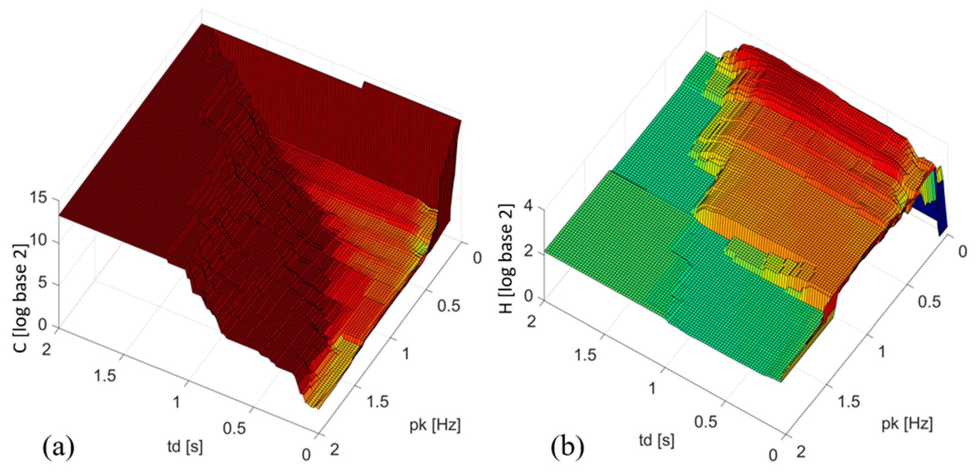
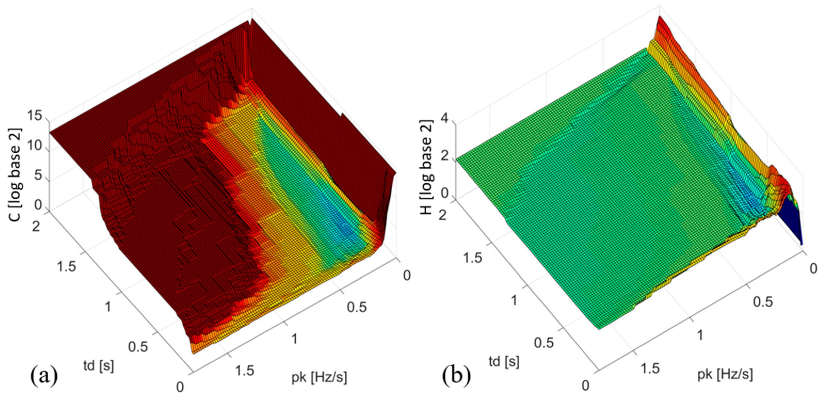
In Figure 12 and Figure 13, the modified entropy (C) and entropy (H) surfaces for the $\mid \Delta f\mid$ feature signal are presented, obtained by exploring the $td$ and $pk$ parameters from 100 × 100 uniformly distributed configurations in a Cartesian plane using the DS 848 02 calculation set. The comparison of the entropy surfaces verifies the hypothesis used to model the modified entropy function presented in Equation (3), where the goal was to penalize non-useful or local minima. The minimum entropy value (H = 0.34602) is only visible in the entropy surface (H), not in the modified entropy surface (C). This occurs because the settings that reach the minimum entropy in surface (H) correspond to a scenario without uncertainty according to the first model but with no practical use for a protection system. However, in the modified entropy model (C), as formulated in Equation (3), these settings are penalized, resulting in higher values.

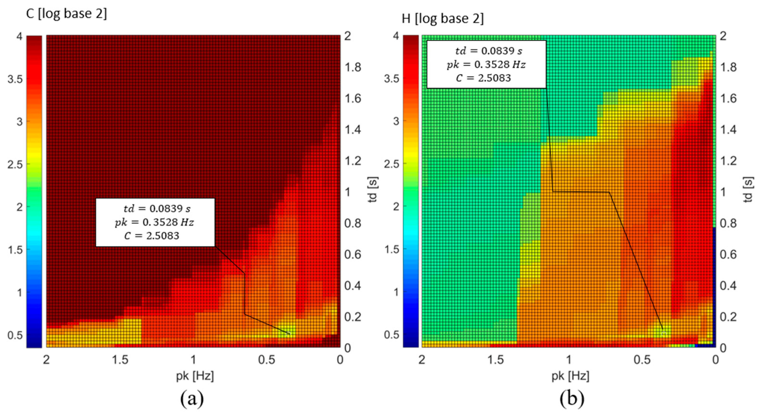
Figure 13 shows the top views of the entropy surfaces from Figure 12, highlighting the optimal settings found. In this region, the surfaces tend to converge, adopting similar shapes and heights. As analyzed in Figure 2, surface (C) gradually aligns with surface (H). For this reason, the uncertainty of the optimal settings is expressed in terms of (C) rather than (H) as they reach identical values at that point. The analysis concludes that (C) improves the surface exploration process, as there are no local or non-useful mathematical minima for protection.

Figure 14 and Figure 15 present the modified entropy (C) and entropy (H) surfaces for the $\mid RoCoF\mid$ feature. These were calculated in the same way as for the $\mid \Delta f\mid$ feature by exploring the $td$ and $pk$ parameters from 100 × 100 = 10,000 uniformly distributed configurations in the defined region of the plane using the DS 848 02 calculation dataset. For the $\mid RoCoF\mid$ feature, the convergence of (C) over (H) near the region of minimal uncertainty is even more evident. Figure 15 illustrates the top views of the entropy surfaces previously shown in Figure 14, highlighting the optimal settings identified on surface (C).

As additional validation of the settings obtained using the BEM, the optimal setting for RoCoF based anti-islanding protection obtained in [29] is presented. This was obtained for the IEEE 34 system using the ASMM (Automatic Setting Map Methodology). Despite differences in the cases, number of events, and optimization methods used in both approaches, the setting achieved using the BEM closely matches that obtained through the ASMM. This result underscores the robustness and effectiveness of the BEM in achieving optimal settings under diverse operating conditions with significant computational savings, as the ASMM used 4606 cases, while the BEM only required 60 cases from the DS 848 02 calculation set.

4.3. Validation Instance

The optimal settings calculated with the BEM, as presented in Table 5, were evaluated using the validation cases from validation datasets. Each of these datasets contains 200 cases, resulting in a total of 1200 validation cases when considering that the detection for each phase is independent (600 island cases and 600 non-island cases). With this large number of cases, it was possible to perform a frequency-based evaluation of detection success and non-detection errors by calculating the probabilities $\widetilde{P_{D/I}}$ and $\widetilde{P_{ND/NI}}$, which represent favorable cases over possible cases. These probabilities are denoted $\widetilde{P_{D/I}}$ and $\widetilde{P_{ND/NI}}$, to differentiate them from the Bayesian inference-based probabilities initially approximated by Bayes estimators, denoted as $p_{D/I}^{\mathrm{*}}$ and $p_{ND/NI}^{\mathrm{*}}$.

In Table 5, where the validation results are presented, the optimal settings for the $\mid RoCoF\mid$ feature from [29] have been included for comparison. The settings obtained using the Bayesian Entropy Methodology (BEM) demonstrate an improvement in terms of both sensitivity and reliability when compared to the previously published adjustments. Specifically, the BEM-derived settings provide a lower entropy value, indicating more robust performance in detecting islanding events while avoiding false detections during non-islanding events.

Furthermore, the settings from [29] (R3) showed higher probabilities of false positives in the non-islanding validation set (DS 848 01), resulting in an increase in entropy values for those configurations. On the contrary, the optimal settings obtained using BEM allowed for better discrimination between islanding and non-islanding scenarios. The pk threshold and optimized td timing in the BEM calibration were crucial in minimizing false detections.

On the other hand, it is clear that the analyzed features are not sufficiently appropriate to achieve an adequate balance between sensitivity and reliability, as they fail to find calibrations with entropy equal to the entropy of the experiment defined by the number of cases considered in the optimal settings calculation dataset (H = C = 0.34602). This suggests that alternative approaches should be explored regarding the use of passive features for island detection with minimal entropy.

The graph presented in Figure 16 illustrates the detection time [s] versus active power imbalance $\Delta P_{island} [\%]$ for the $\mid RoCoF\mid$ feature under Generation Scenario 1, where the island is formed with 75% synchronous generation (DG1) and 25% converter-based generation (DG2). The results compare three calibrations: R1 obtained using the BEM and R2 and R3 obtained from ASMM [29]. The x-axis represents the active power imbalance, with negative values corresponding to power deficits and positive values to power excess. The y-axis denotes the detection time in seconds.

The three-phase responses for each calibration are plotted, where R1 (in red) shows a detection time slightly longer than that obtained with calibration R3 but much better than calibration R2, which failed to detect any of these cases satisfactorily. Calibration R3 demonstrates a similar performance to R1 but exhibits slightly more sensitivity with a lower pk setting, although at the cost of increased false detections in other validation scenarios (disturbances), which reduces the probability of avoiding erroneous detections and increases the measured entropy in the validation set, as presented in

Table 6. Validation results.

Feature	Evaluated Setting	C/H (Calculation)	Optimal $\mathit{t}\mathit{d}$	Optimal $\mathit{p}\mathit{k}$	$\widetilde{{\mathit{P}}_{\mathit{D}/\mathit{I}}}$	$\widetilde{{\mathit{P}}_{\mathit{N}\mathit{D}/\mathit{N}\mathit{I}}}$	H (Validation)
$\left|∆f\right|$	F1	2.5083	0.0839 s	0.3528 Hz	0.851	0.851	2.42
$\mid RoCoF\mid$	R1(BEM)	1.4619	0.4226 s	0.1788 Hz/s	0.866	1	1.09
	R2 [29]	-	0.16 s	1 Hz/s	0.235	1	1.774
	R3 [29]	-	0.355 s	0.150 Hz/s	0.885	0.988	1.23
$\left|∆\mathrm{U}\right|$	U1	3.7909	0.1818 s	0.50505 V	0.348	0.865	3.344
$\left|RoCoV\right|$	RV1	2.1532	0.0404 s	0.50505 KV/s	0.973	0.465	1.891
THD %	T1	0.7760	1.8384 s	2.0202%	0.756	0.695	3.38

.

Similarly to Figure 16, Figure 17 presents the detection time [s] versus the active power imbalance $\Delta P_{island} [\%]$ for the $\mid RoCoF\mid$ feature under Generation Scenario 2, which consists of a 50% synchronous generation and 50% converter-based generation mix.

In this scenario, the $\mid RoCoF\mid$ feature calibrated with R1 (in red) consistently shows a detection time slightly longer than that obtained with calibration R3. Due to the generation scenario, it can be observed that the NDZ has been reduced, as under this hypothesis of island formation (generation Scenario 2), the formed islands have less inertia, and the frequency deviations are much more pronounced than in Scenario 1, facilitating detection.

Regarding generation Scenario 3, the detection time graph has been omitted, but the obtained results are very similar to those of the previous two scenarios, showing a complete reduction in the non-detection zones for all three calibrations. In this generation scenario, it was possible to detect all island cases present in the validation set.

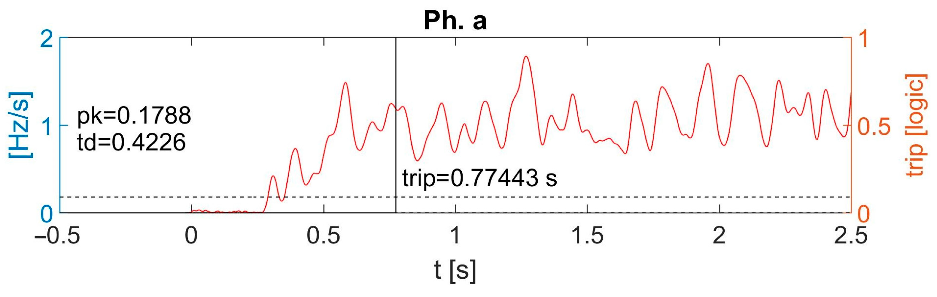
Figure 18 presents the detection test for calibration R1 obtained using the BEM in an island case corresponding to generation Scenario 3. Significant frequency deviations can be observed for small active and reactive power imbalances $\Delta P_{island}$ and $\Delta Q_{island}$ obtained in this case. These large frequency deviations are due to the reduced inertia of the island formed under the case’s conditions.

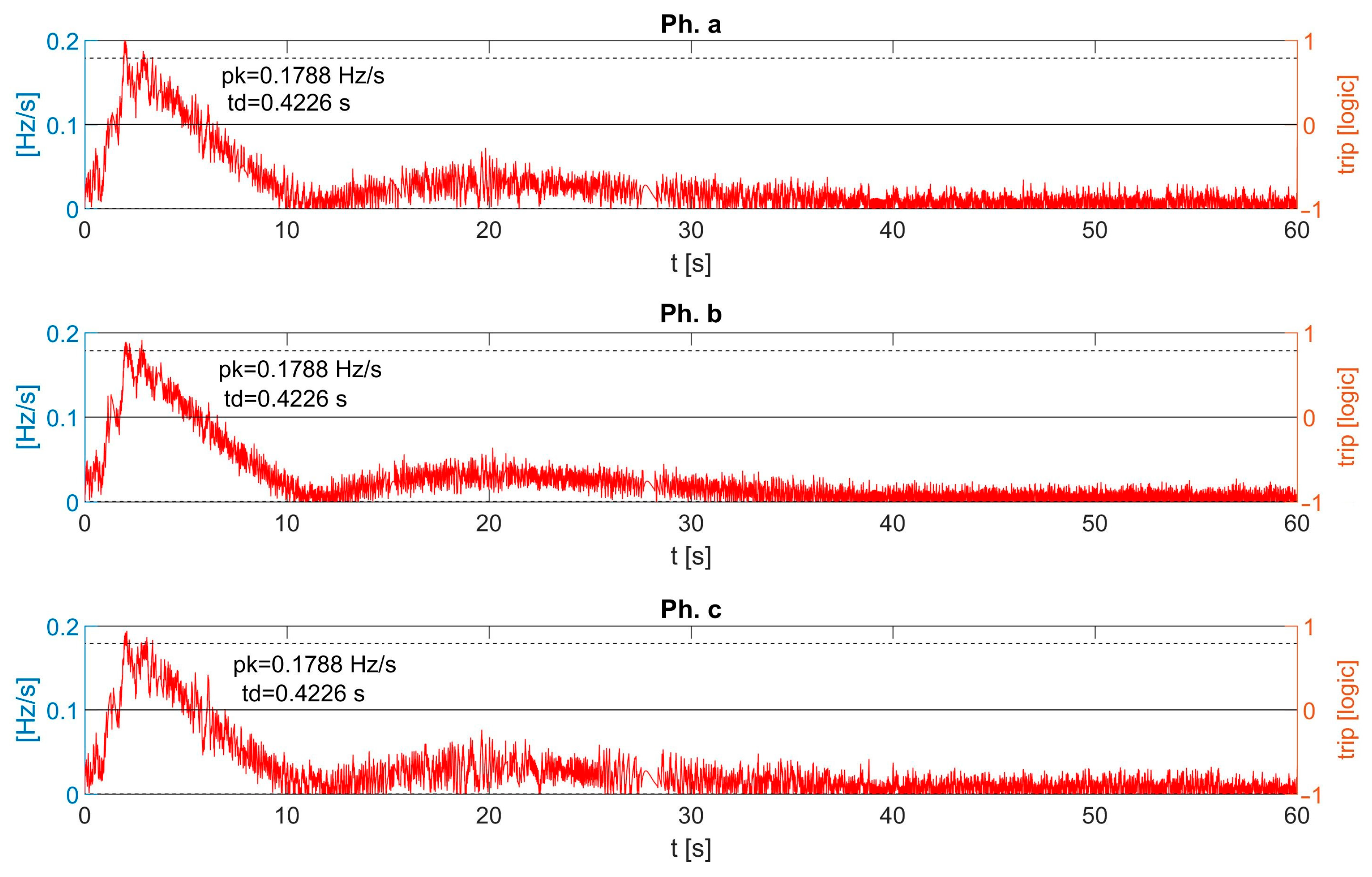
Finally, Figure 19 illustrates the detection signals for $\mid RoCoF\mid$ calibration R1, using the BEM in all three phases for a severe disturbance case (disturbance_189) from the validation dataset. In this scenario, the generator GA is disconnected, resulting in a significant disturbance with a power imbalance $\Delta P_{BPS}=-90 \mathrm{M}\mathrm{W}$ and a maximum rate of change of frequency $RoCo{F}_{max}\approx -0.1907 \mathrm{H}\mathrm{z}/\mathrm{s}$, which exceeds the threshold of the optimal calibration found by the BEM ($pk=0.1788 \mathrm{H}\mathrm{z}/\mathrm{s}$, $pk=0.4226 \mathrm{s}$). Despite this, the optimal calibration obtained with the BEM avoids triggering the protection, demonstrating an appropriate balance between sensitivity and reliability.

This is a critical observation, as the calibration successfully detects the severe disturbance while preventing false positives, which is a key performance indicator for protection systems. Moreover, the NDZ for the BEM-calibrated protection is similar to the calibration R3 obtained using ASMM. However, the BEM calibration is much more reliable, as it did not falsely trigger for any disturbances in the validation dataset. This highlights the superiority of the BEM method, providing both accurate detection of islands and robust protection against false alarms under various disturbance conditions, while also significantly reducing the number of cases analyzed in the dataset compared to the ASMM. The BEM achieves reliable calibrations with reduced dataset, optimizing the process and saving computational effort without compromising detection accuracy.

5. Conclusions

This work successfully demonstrated the effectiveness of the Bayesian Entropy Methodology (BEM) for optimizing the calibration settings of anti-islanding protections. The results highlight the BEM’s ability to identify optimal settings for sensitivity and reliability using a significantly reduced dataset compared to other methodologies.

Table 7. Comparison of simulation dataset size and minimum entropy achieved with other islanding detection works.

Work	IDM	Dataset Size	${{\mathit{p}}_{\mathit{D}/\mathit{I}}^{\mathbf{*}}}_{\mathit{M}\mathit{A}\mathit{X}}$	${{\mathit{p}}_{\mathit{N}\mathit{D}/\mathit{N}\mathit{I}}^{\mathbf{*}}}_{\mathit{M}\mathit{A}\mathit{X}}$	Equivalent Achievable Entropy
Current Work: (BEM)	$\left|∆f\right|$, $\left|∆\mathrm{U}\right|$, $\mid RoCoF\mid$ $\left|RoCoV\right|$ THD %	60	0.9891	0.9891	0.34602
Setting Map Methodology (SMM) [29,30]	RoCoF	4606	0.9786	0.9902	0.4568
Pattern Recognition Approach [25]	Wavelet Decision Tree classifier	2091	0.9765	0.9520	0.8752
Wavelets and Deep Learning Methodology (WDLM) [26]	Wavelet Deep Learning	2046	0.9891	0.9855	0.3915
Reliable Islanding Detection Scheme (RIDS) [27]	Modified Intrinsic Mode Functions (MIMF)	720	0.9740	0.9859	0.5672

presents a comparison of the amount of data required in other works published in the literature. Notably, BEM required only 60 cases in the calculation dataset to achieve settings comparable to other works. This reduction represents a substantial saving in computational effort.

This work has also demonstrated the advantages of using the modified entropy function over the entropy function. The modified entropy allows for the elimination of low-uncertainty regions that have no practical application in protection systems. This improvement paves the way for future research to automate the search for calibration regions with minimal uncertainty through an optimization algorithm. This approach reduces the risk of “falling into erroneous zones” with mathematically low entropy but lacking real physical relevance. Consequently, the modified entropy function enhances the robustness and reliability of the search process for optimal calibration settings in protection systems.

The validation of the optimal settings against various disturbance and islanding scenarios confirmed that the BEM-derived settings provide a robust balance between sensitivity and reliability. The reduced non-detection zones (NDZs) and avoidance of false tripping across all tested conditions underscore the method’s superiority in maintaining operational reliability, even under severe power system disturbances.

Future work will focus on exploring combinations of characteristic signals to improve detection performance further. Investigating the potential for multi-signal feature fusion, such as integrating RoCoF with other features, may yield an even more sensitive and reliable detection signal. This approach could lead to the development of a composite detection algorithm that leverages the strengths of multiple features, thereby reducing entropy to even lower levels and improving the overall robustness of passive anti-islanding protections.

In conclusion, the BEM offers a novel, computationally efficient approach to optimizing anti-islanding protections. By incorporating additional signals and enhancing feature combinations in future work, there is significant potential to improve the detection accuracy and reliability of islanding protections in increasingly complex distribution networks with high DER penetration.

References

1. Conti, S. Analysis of Distribution Network Protection Issues in Presence of Dispersed Generation. Electr. Power Syst. Res. 2009, 79, 49–56. [Google Scholar] [CrossRef]
2. Stevens, J.; Bonn, R.; Gin, J.; Gonzalez, S.; Greg, K. Development and Testing of an Approach to Anti-Islanding in Utility-Interconnected Photovoltaic Systems; Sandia National Lab. (SNL-NM): Albuquereque, NM, USA, 2000. [Google Scholar]
3. Kou, G.; Deverick, J.; Phelps, K.; Nguyen, T.; Velez-Cedeno, F.G. Impact of Distributed Energy Resources on Arc Flash Incident Energy. IEEE Trans. Power Deliv. 2020, 35, 531–539. [Google Scholar] [CrossRef]
4. Pazos, F.J. Operational Experience And Field Tests On Islanding Events Caused By Large Photovoltaic Plants. In Proceedings of the CIRED 21st International Conference on Electricity Distribution, Frankfurt, Germany, 6–9 June 2011; pp. 1–4. [Google Scholar]
5. IEEE Std 1547-2018; IEEE Standard for Interconnection and Interoperability of Distributed Energy Resources with Associated Electric Power Systems Interfaces. IEEE: Piscataway, NJ, USA, 2018; pp. 1–138. [CrossRef]
6. Chowdhury, S.P.; Chowdhury, S.; Crossley, P.A. UK Scenario of Islanded Operation of Active Distribution Networks with Renewable Distributed Generators. Int. J. Electr. Power Energy Syst. 2011, 33, 1251–1255. [Google Scholar] [CrossRef]
7. Energy Networks Association. The Distribution Code of Licensed Distribution Network Operators of Great Britain; Energy Networks Association: London, UK, 2023. [Google Scholar]
8. European Union Commission. Commission Regulation (Eu) 2016/631 of 14 April 2016 Establishing a Network Code on Requirements for Grid Connection of Generators; Official Journal of the European Union: Luxembourg, 2016.
9. Hatziargyriou, N.; Abbey, C.; Alabbas, A.; Barsali, S.; Belhomme, R.; Bruendlinger, R.; Daae, S.; Dizdarevic, N.; Driesen, J.; Funabashi, T.; et al. Connection Criteria at the Distribution Network for Distributed Generation; CIGRE Task Force C6.04.01; CIGRE: Paris, France, 2007; ISBN 978-285873-001-8. [Google Scholar]
10. Dyśko, A.; Booth, C.; Burt, A.G.; Yip, H.T. Testing Methodology for LOM Protection Performance Assessment. In Proceedings of the 10th IET International Conference on Developments in Power System Protection (DPSP 2010), Manchester, UK, 29 March–1 April 2010. [Google Scholar]
11. MacIver, C.; Bell, K.; Nedd, M. An Analysis of the August 9th 2019 GB Transmission System Frequency Incident. Electr. Power Syst. Res. 2021, 199, 107444. [Google Scholar] [CrossRef]
12. NERC. 2023 Southwest Utah Disturbance; NERC: Atlanta, GA, USA, 2023. [Google Scholar]
13. Mishra, M.; Chandak, S.; Rout, P.K. Taxonomy of Islanding Detection Techniques for Distributed Generation in Microgrid. Renew. Energy Focus 2019, 31, 9–30. [Google Scholar] [CrossRef]
14. Abu Sarhan, M. An Extensive Review and Analysis of Islanding Detection Techniques in DG Systems Connected to Power Grids. Energies 2023, 16, 3678. [Google Scholar] [CrossRef]
15. ANSI C37.2-1996; IEEE Standard for Electrical Power System Device Function Numbers. Institute of Electrical and Electronics Engineers: New York, NY, USA, 1996.
16. Arguence, O.; Cadoux, F.; Raison, B.; De Alvaro, L. Non-Detection Zone of an Anti-Islanding Protection with Rate of Change of Frequency Threshold. CIRED—Open Access Proc. J. 2017, 2017, 1338–1341. [Google Scholar] [CrossRef]
17. Vieira, J.C.M.; Freitas, W.; Huang, Z.; Xu, W.; Morelato, A. Formulas for Predicting the Dynamic Performance of ROCOF Relays for Embedded Generation Applications. IEE Proc.—Gener. Transm. Distrib. 2006, 153, 399. [Google Scholar] [CrossRef]
18. Patsidis, A.; Tzelepis, D.; Dyśko, A.; Booth, C. Investigation of the Performance of ROCOF-Based Lom Protection in Distribution Networks with Virtual Synchronous Generators. In Proceedings of the 15th International Conference on Developments in Power System Protection (DPSP 2020), Liverpool, UK, 10–12 March 2020; Institution of Engineering and Technology: Stevenage, UK, 2020; p. 6. [Google Scholar]
19. Dysko, A.; Tzelepis, D.; Booth, C. Assessment of Risks Resulting from the Adjustment of Vector Shift (VS) Based Loss of Mains Protection Settings; University of Strathclyde: Glasgow, UK, 2017. [Google Scholar]
20. Western-Power-Distribution. Loss of Mains Protection—Distribution System Operability Framework June 2018; Western-Power-Distribution: Bristol, UK, 2018; pp. 1–10. [Google Scholar]
21. Ropp, M.E.; Begovic, M.; Rohatgi, A. Prevention of Islanding in Grid-Connected Photovoltaic Systems. Prog. Photovolt. Res. Appl. 1999, 7, 39–59. [Google Scholar] [CrossRef]
22. Vieira, J.C.M.; Freitas, W.; Xu, W.; Morelato, A. An Investigation on the Nondetection Zones of Synchronous Distributed Generation Anti-Islanding Protection. IEEE Trans. Power Deliv. 2008, 23, 593–600. [Google Scholar] [CrossRef]
23. Salles, D.; Freitas, W.; Vieira, J.C.M.; Venkatesh, B. A Practical Method for Nondetection Zone Estimation of Passive Anti-Islanding Schemes Applied to Synchronous Distributed Generators. IEEE Trans. Power Deliv. 2015, 30, 2066–2076. [Google Scholar] [CrossRef]
24. Salles, D.; Freitas, W.; Vieira, J.C.M.; Xu, W. Nondetection Index of Anti-Islanding Passive Protection of Synchronous Distributed Generators. IEEE Trans. Power Deliv. 2012, 27, 1509–1518. [Google Scholar] [CrossRef]
25. Lidula, N.W.A.; Rajapakse, A.D. A Pattern-Recognition Approach for Detecting Power Islands Using Transient Signals-Part II: Performance Evaluation. IEEE Trans. Power Deliv. 2012, 27, 1071–1080. [Google Scholar] [CrossRef]
26. Allan, O.A.; Morsi, W.G. A New Passive Islanding Detection Approach Using Wavelets and Deep Learning for Grid-Connected Photovoltaic Systems. Electr. Power Syst. Res. 2021, 199, 107437. [Google Scholar] [CrossRef]
27. Chaitanya, B.K.; Yadav, A.; Pazoki, M. Reliable Islanding Detection Scheme for Distributed Generation Based on Pattern-Recognition. IEEE Trans. Ind. Informatics 2021, 17, 5230–5238. [Google Scholar] [CrossRef]
28. Kulkarni, N.K.; Khedkar, M.K. Methods to Detect the Occurrence of an Unintentional Island with Passive Approach: A Review. J. Inst. Eng. Ser. B 2021, 102, 1091–1111. [Google Scholar] [CrossRef]
29. Motter, D.; De Melo Vieira, J.C. The Setting Map Methodology for Adjusting the DG Anti-Islanding Protection Considering Multiple Events. IEEE Trans. Power Deliv. 2018, 33, 2755–2764. [Google Scholar] [CrossRef]
30. Motter, D.; Vieira, J.C.M. Improving the Islanding Detection Performance of Passive Protection by Using the Undervoltage Block Function. Electr. Power Syst. Res. 2020, 184, 106293. [Google Scholar] [CrossRef]
31. Andrade Mourinho, F.; Mariano Lessa Assis, T. Impact of Cascade Disconnection of Distributed Energy Resources on Bulk Power System Stability: Modeling and Mitigation Requirements. J. Mod. Power Syst. Clean Energy 2023, 11, 412–420. [Google Scholar] [CrossRef]
32. Seguin Batadi, E.M.; Martínez, M.; Molina, M.G. Bayesian Entropy Methodology: A Novel Approach to Setting Anti-Islanding Protections with Enhanced Stability and Sensibility. Energies 2024, 17, 693. [Google Scholar] [CrossRef]
33. Shannon, C.E. A Mathematical Theory of Communication. Bell Syst. Tech. J. 1948, 27, 379–423. [Google Scholar] [CrossRef]
34. Kersting, W.H. Radial Distribution Test Feeders. IEEE Trans. Power Syst. 1991, 6, 975–985. [Google Scholar] [CrossRef]
35. Mwakabuta, N.; Sekar, A. Comparative Study of the IEEE 34 Node Test Feeder under Practical Simplifications. In Proceedings of the 2007 39th North American Power Symposium, Las Cruces, NW, USA, 30 September–2 October 2007; IEEE: Piscataway, NJ, USA, 2007; pp. 484–491. [Google Scholar]
36. Owuor, A.J.O.; Munda, J.L.; Jimoh, A.A. The IEEE 34 Node Radial Test Feeder as a Simulation Testbench for Distributed Generation. In Proceedings of the IEEE Africon ’11, Livingstone, Zambia, 13–15 September 2011; IEEE: Piscataway, NJ, USA, 2011; pp. 1–6. [Google Scholar]
37. de Barros Iscuissati, R.; Motter, D.; José, J.C. Probabilistic Method for Risk Analysis of Unintentional Islanding of Distributed Generators. Electr. Power Syst. Res. 2024, 234, 110594. [Google Scholar] [CrossRef]
Figure 1. Simplified model of the anti-islanding protection, considering it as an element that extracts a feature signal and applies threshold violation detection defined by the settings time-delay (td) and pickup (pk).
Sustainability 17 04859 g001
Figure 2. Error surfaces when approximating entropy (H) using (C). Adjustment parameters: surface (a):   k = 1000 ,     a = 0.35 ; surface (b): = 1 ,     a = 0.5 .
Sustainability 17 04859 g002
Figure 3. Comparison of entropy surfaces (H) and modified entropy (C) as a function of forward success probabilities: p D / I and p N D / N I . Adjustment parameters of modified entropy: k = 1000   a = 0.35 .
Sustainability 17 04859 g003
Figure 4. Bayesian Entropy Methodology (BEM) flowchart with the implementation of modified entropy calculation. p D / I and p N D / N I are probabilities estimated using Bayesian inference.
Sustainability 17 04859 g004
Figure 5. Test system with the addition of two generators at Node 848: a synchronous generator and an inverter-based generator. The diagram illustrates the locations of the faults and the islanding scenarios considered for the random case selection.
Sustainability 17 04859 g005
Figure 6. Single-line diagram of the BPS connected to the IEEE 34-node system.
Sustainability 17 04859 g006
Figure 7. DPL codes to generate datasets of cases for calculation and validation.
Sustainability 17 04859 g007
Figure 8. Signal extraction process at Node 848-B. (a) Frequency and RoCoF calculations. (b) Voltage deviation and RoCoV calculations. (c) Total Harmonic Distortion (THD) calculation.
Sustainability 17 04859 g008
Figure 9. Results of the calculation in phase ‘a’ of the characteristics f and R o C o F . Islanding event at Node 848, Generation Scenario 848:2 (50% synchronous generation, 50% converters). IEEE 34: sixth demand scenario. Island formed by the disconnection of the 834–842 line at t = 0.25 s. P i s l a = + 15.87 % , Q i s l a = + 29.77 % .
Sustainability 17 04859 g009
Figure 10. (a) Side view of the modified entropy surface (C) for the R o C o V feature obtained through exploration for 0 p k 2   k V / s and 0 t d 2   s .   (b) Side view of the modified entropy surface (C) for the U feature obtained through exploration for 0 p k 0.05   k V and 0 t d 2   s .
Sustainability 17 04859 g010
Figure 11. (a) Side view of modified entropy surface (C) for the THD feature obtained through exploration for 0 p k 100 % and 0 t d 2   s . (b) Detail of the obtained marginal calibration. Dataset DS 848 02.
Sustainability 17 04859 g011
Figure 12. Side views for the f feature obtained through exploration for 0 p k 2   H z and 0 t d 2   s   (a) Modified entropy surface (C). (b) Entropy surface (H). dataset DS 848 02.
Sustainability 17 04859 g012
Figure 13. Top views and optimal settings obtained for the f feature obtained through exploration for 0 p k 2   H z and 0 t d 2   s   (a) Modified entropy surface (C). (b) Entropy surface (H). Dataset DS 848 02.
Sustainability 17 04859 g013
Figure 14. Side views and for the R o C o F feature obtained through exploration for 0 p k 1.8   H z / s and 0 t d 2   s   (a) Modified entropy surface (C). (b) Entropy surface (H). Dataset DS 848 02.
Sustainability 17 04859 g014
Figure 15. Top views and settings obtained for the R o C o F feature obtained through exploration for 0 p k 1.80 and 0 t d 2 . (a) Modified entropy surface (C). (b) Entropy surface (H). Legend (1): Optimal settings found using the BEM. Legend (2): Optimal settings proposed in [29]. Dataset DS 848 02.
Sustainability 17 04859 g015
Figure 16. R o C o F detection time [s] vs. Δ P i s l a n d . Calibration R1: BEM; calibrations R2 and R3: ASMM [29]. Sixty-nine cases from the validation dataset. Generation scenario for Node 848 number 1: 75% synchronous generation—25% converters. (Cases with zero detection time correspond to undetected island cases).
Sustainability 17 04859 g016
Figure 17. R o C o F detection time [s] vs. Δ P i s l a n d . Calibration R1: BEM; calibrations R2 and R3: ASMM [29]. Sixty-four cases from the validation dataset. Generation scenario for Node 848 number 2: 50% synchronous generation—50% converters. (Cases with zero detection time correspond to undetected island cases).
Sustainability 17 04859 g017
Figure 18. Detection test for R o C o F . Calibration R1 (BEM) in phase ‘a’, case: island_181 from the validation dataset. Generation Scenario 848: 3 (25% synchronous generation, 75% converters). IEEE 34 Demand Scenario: 7. Island formed by opening the 834–842 line at t = 0.25 . P i s l a n d = 0.7 % , Q i s l a n d = + 5.36 % .
Sustainability 17 04859 g018
Figure 19. Detection signals for R o C o F —R1 (BEM) in all three phases for case: disturbance_189 from the disturbance validation dataset. Disconnected generator: GA. Disturbance time t = 1   s   Δ P B P S = 90   M W , H B P S = 8.40   s , S B P S = 1566.9   M V A , R o C o F m a x 0.1907   H z . Demand Scenario SSEE: 8 (70–80%). Generation Scenario: 1 (renewable participation equal to 10.12%).
Sustainability 17 04859 g019