An Innovative Framework for Forecasting the State of Health of Lithium-Ion Batteries Based on an Improved Signal Decomposition Method

Abstract

The declining trend of battery aging has strong nonlinearity and volatility, which poses great challenges to the prediction of battery’s state of health (SOH). In this research, an innovative framework is initially put forward for SOH prediction. First, partial incremental capacity analysis (PICA) is carried out to analyze the performance degradation within a specific voltage range. Subsequently, the height of the peak, the position of the peak, and the area beneath the peak of the IC curves are retrieved and used as health features (HFs). Moreover, improved ensemble empirical mode decomposition based on fractal dimension (FEEMD) is first proposed and utilized to decompose HFs to reduce the nonlinearity and fluctuations. Additionally, a bidirectional gated recurrent unit with an attention mechanism (BiGRU-AM) is constructed for the prognosis of these sub-layers. Finally, the effectiveness and robustness of the proposed prognosis framework are validated using two battery datasets. The results of three groups of comparative experiments demonstrate that the maximum root mean squared error (RMSE) and mean absolute error (MAE) values reach merely 0.55% and 0.59%, respectively. This further demonstrates that the proposed FEEMD outperforms other benchmark models and can offer a reliable foundation for the health prognosis of lithium-ion batteries.

1. Introduction

1.1. Motivation

After the Industrial Revolution, the traditional fossil energy represented by coal faced a certain degree of reserve crisis because of its large-scale exploitation. The emergence and utilization of new energy can alleviate the harm to the ecological environment caused by human beings. Lithium-ion batteries (LIBs), as the representative of energy storage devices, have been widely exploited in household appliances, electric vehicles, urban transportation, and spacecraft [1,2]. In the power grid, LIBs are utilized in energy storage power plants, which effectively improves the ability of the grid to absorb renewable energy. Nevertheless, when LIBs have internal faults, it is very easy to cause runaway heating, major accidents, and even endanger the safety of public life and property. Therefore, it is highly significant to set up an intelligent and efficient battery management system (BMS) for the purpose of monitoring the safety and reliability of batteries. As a crucial state parameter of batteries, the estimation of state of health (SOH) has long been a central concern in battery management systems (BMSs) and a technical challenge that needs to be addressed concurrently, as indicated in references [1,3]. The pursuit of higher energy density has driven the development of advanced anode materials, such as silicon (Si)-based anodes and silicon oxide (SiOx) anodes, which offer theoretical capacities an order of magnitude higher than commercial graphite. Silicon anodes face severe challenges from volumetric expansion during lithiation/delithiation, leading to mechanical degradation and unstable solid–electrolyte interfaces (SEIs) in both liquid and solid electrolyte systems. For SiOx anodes, while their specific capacity and reduced volume change compared to pure Si make them promising, they suffer from metastable structural evolution, continuous SEI reconstruction, and irreversible lithium consumption. These material-level issues introduce complex nonlinearities in battery degradation profiles, particularly when paired with sulfide-based solid-state electrolytes (SSEs), where mechanical instability and interfacial chemical reactions further exacerbate capacity fade [4,5].

1.2. Literature Review

Based on relevant research results at home and abroad, the common techniques for estimating the battery’s SOH can be mainly categorized into two types: model-based methods and data-driven approaches.

Model-based methods, such as electrochemical models (EM) [4] and equivalent circuit models (ECM) [5], struggle to capture the intricate electrochemical–mechanical interactions in advanced anode systems. For example, in sulfide SSE systems with Si anodes, external pressure and binder properties significantly influence interfacial stability, creating nonlinear degradation patterns that exceed the simplifying assumptions of traditional models. Similarly, the crystallographic engineering of SiOx anodes via lithium fluoride (LiF) treatment introduces quartz-like phases that enhance mechanical integrity and mitigate irreversible lithium loss, highlighting the role of microstructural design in stabilizing anode–electrolyte interfaces. These advancements emphasize that novel material systems, while promising for high energy density, demand sophisticated signal processing and machine learning frameworks to address their unique degradation dynamics [6,7]. The EM provides an understanding of the internal dynamic processes within batteries. The most commonly utilized model is the pseudo-two-dimensional (P2D) model. For instance, Boyan et al. [8] performed a joint estimation of the state of charge (SOC) and SOH using a P2D model and confirmed that the estimation error was below 3%. Nevertheless, the high computational requirements and the complexity of the control equations needed for this approach have an impact on its reliability and practical application. The ECM determines parameters by constructing a suitable equivalent circuit. SOH is typically reflected indirectly through some filter-based techniques such as the Particle Filter (PF), Unscented Particle Filter (UPF), and Unscented Kalman Filter (UKF). For instance, Liu et al. [9] proposed an improved lithium-ion battery degradation algorithm, considering the circulating current. The algorithm employs genetic techniques to determine the initial values of model parameters and develops a PF to track the variations in parameters and states. Experimental results demonstrate that the root mean square error of SOH and RUL forecasting is less than 8% and 40 cycles, respectively, proving the method’s applicability. Shen et al. [10] explored the nonlinear Wiener process to establish the capacity deterioration process and estimated the model parameters online by UPF. Shi et al. [11] proposed a second-order resistance–capacitance (RC) ECM to estimate the SOH. In their approach, an improved UPF was utilized for SOH estimation, while a UKF was employed to generate the importance probability density function for the PF. Although the ECM-based estimation method provides high accuracy, its performance is highly sensitive to the precision of the underlying model. This characteristic renders it unsuitable for online applications. In general, the effectiveness and applicability of model-based methods largely depend on multiple parameters, such as charge/discharge current, temperature, and voltage. These parameters significantly influence the accuracy of model predictions, as they are closely related to the dynamic electrochemical processes and degradation mechanisms within batteries. Precise parameter acquisition and reasonable selection are crucial for improving the reliability of model-based SOH estimation methods. These factors can have a substantial impact on the prediction performance of the battery. Constructing a proper battery aging model is no simple task. Consequently, model-based approaches are not optimal for practical scenarios.

With the booming development of artificial intelligence, data-driven methods for predicting the SOH have drawn widespread attention. In contrast, these data-driven prediction methods establish a mapping connection between external features and SOH without considering a great deal of prior knowledge or the internal mechanism. In general, SOH prediction based on data-driven methods can be broken down into two steps: feature extraction and estimation using deep-learning algorithms. Lately, the most intensively studied method is incremental capacity analysis (ICA) [12]. To enhance the assessment of the SOH, a comprehensive set of features is extracted from IC curves, including peak area [13], peak height, and peak position [14,15]. Unlike voltage curves, IC curves provide more detailed insights into battery aging, largely because they are more sensitive to the specific electrochemical reactions occurring within the battery [16]. However, when considering actual applications, it is rather challenging to ensure the completeness of the charging and discharging process for lithium-ion batteries. Thus, some research has directly derived health indicators from partial incremental capacity analysis (PICA). For example, Li et al. [17] derived battery health indexes from segments of the IC curves. These indexes were then employed as the input data for the battery degradation model. Through experimental verification, the proposed approach demonstrated its effectiveness, with both the MAEs and RMSEs remaining below 2%. However, the original partial IC curves are replete with too much noise to be directly applied to SOH prediction. This challenge has motivated numerous researchers to apply various filtering techniques to smooth IC curves, such as the moving average (MA) method [18]. Nevertheless, the efficacy of MA filtering largely hinges on the fixed window size: while a larger window can produce smoother curves, it may also distort the IC curve, leading to potential misinterpretation of critical features. Thus, the window size must be carefully optimized within a suitable range, a process that can be quite time-consuming. As a result, an advanced filtering algorithm named wavelet filtering (WF) is utilized in this investigation.

Even though the extraction of features from partial IC curves shows effectiveness, certain drawbacks are still present, such as the nonlinearity and fluctuations of the features, which will heavily influence the accuracy of the SOH prediction. Since it has also shown that the signal processing strategies can effectively remove the non-stationary and nonlinearity in HFs, it will be investigated in this paper. Among signal processing techniques, empirical mode decomposition (EMD) has emerged as a mainstream method. Moreover, numerous advanced derivatives have been thoroughly investigated, including ensemble empirical mode decomposition (EEMD) and complementary ensemble empirical mode decomposition (CEEMD). EMD [19] is commonly employed to break down non-stationary signals into a limited number of sub-layers. However, mode aliasing is a common issue in EMD, where a single intrinsic mode function (IMF) may contain components with different time scales. To address this, EEMD [20] introduces Gaussian white noise to mitigate mode aliasing but still suffers from significant reconstruction errors. CEEMD [21] further improves this by adding pairs of positive and negative white noise, yet it can generate false components and increase computational complexity. To overcome these limitations, this study proposes and employs an improved method—fractal dimension-based ensemble empirical mode decomposition (FEEMD)—to decompose the extracted HFs for the first time.

With the booming progress of deep learning, a variety of algorithms have been implemented in the battery degradation model. These methods include support vector machine (SVR), Gaussian process regression (GPR), and multiple linear regression (MLR). SVR [22] linearizes complex nonlinear problems by increasing dimensionality, but it is highly sensitive to parameters, missing data, and kernel functions. GPR [23,24,25] is a common supervised learning approach that can handle probabilistic problems, yet it often struggles with high-dimensional feature spaces. MLR [26] can quickly compute linear correlations among factors but is limited in solving complex nonlinear problems. In the realm of deep learning, recurrent neural networks (RNNs) are valuable for managing random time series, but their inability to handle long-distance information can lead to issues like gradient vanishing [27]. The gated recurrent unit (GRU), an advanced version of RNN, effectively addresses long-term dependencies, mitigating the gradient vanishing problem in traditional RNNs and making it more suitable for sequence data [28]. However, in lithium-ion battery degradation sequences, the current output has both forward and backward time correlations. To overcome the drawbacks of the traditional GRU, Zhu et al. [29] constructed a bidirectional gated recurrent unit (BiGRU) network for subseries prognosis and attained relatively high forecasting accuracy. However, the above-mentioned GRU-based prediction algorithms do not take into account the disparities in the importance of sequence features. As a result, some crucial features might be neglected, causing a decline in the predicted performance. Yu et al. [30] incorporated the bidirectional gated recurrent unit with an attention mechanism (BiGRU-AM). This mechanism was used to allocate distinct weights to the hidden states within BiGRU, thereby highlighting the influence of crucial information. Eventually, the experimental outcome demonstrated that the proposed model could further improve the prediction accuracy. Motivated by this achievement, in this research, the BiGRU-AM is applied to the domain of SOH forecasting for lithium-ion batteries.

1.3. Contribution

To address the aforementioned challenges, this research proposes an innovative hybrid data-driven architecture for prognosticating the SOH. The key innovations and contributions of this study can be elaborated as follows:

(1) Two filtering methods are used to smooth the battery IC curves, and the superior approach is then selected for curve fitting;

(2) Significant health features (peak height, peak position, and area) are extracted from partial IC curves in the main battery charging region;

(3) In order to decrease the nonlinearity and fluctuations in HFs, FEMMD is first proposed and introduced to decompose the HFs into a series of sub-layers, which has never been investigated in SOH forecasting before;

(4) The BiGRU-AM is utilized for predicting sub-layers. This mechanism adjusts weights for GRU layers, prioritizing key information to enhance the accuracy of SOH predictions;

(5) Three comparative experiments were carried out to validate the performance and superiority of the proposed hybrid model.

1.4. Organization of the Paper

The organization of the paper is constructed as follows: Section 2 presents basic methods for incremental capacity curve analysis and smoothing technique, feature extractions from the ICA, FEEMD, and BiGRU-AM. The proposed scheme is detailed in Section 3. Section 4 presents the experimental study using two battery datasets and compares the forecasting results of different models. The key conclusions are summarized in the final section.

2. Methodology

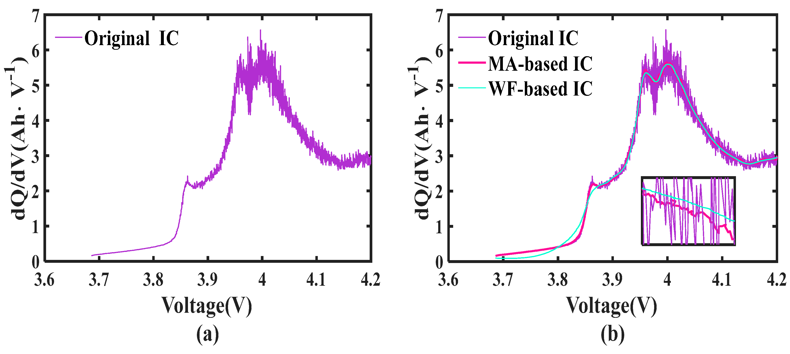
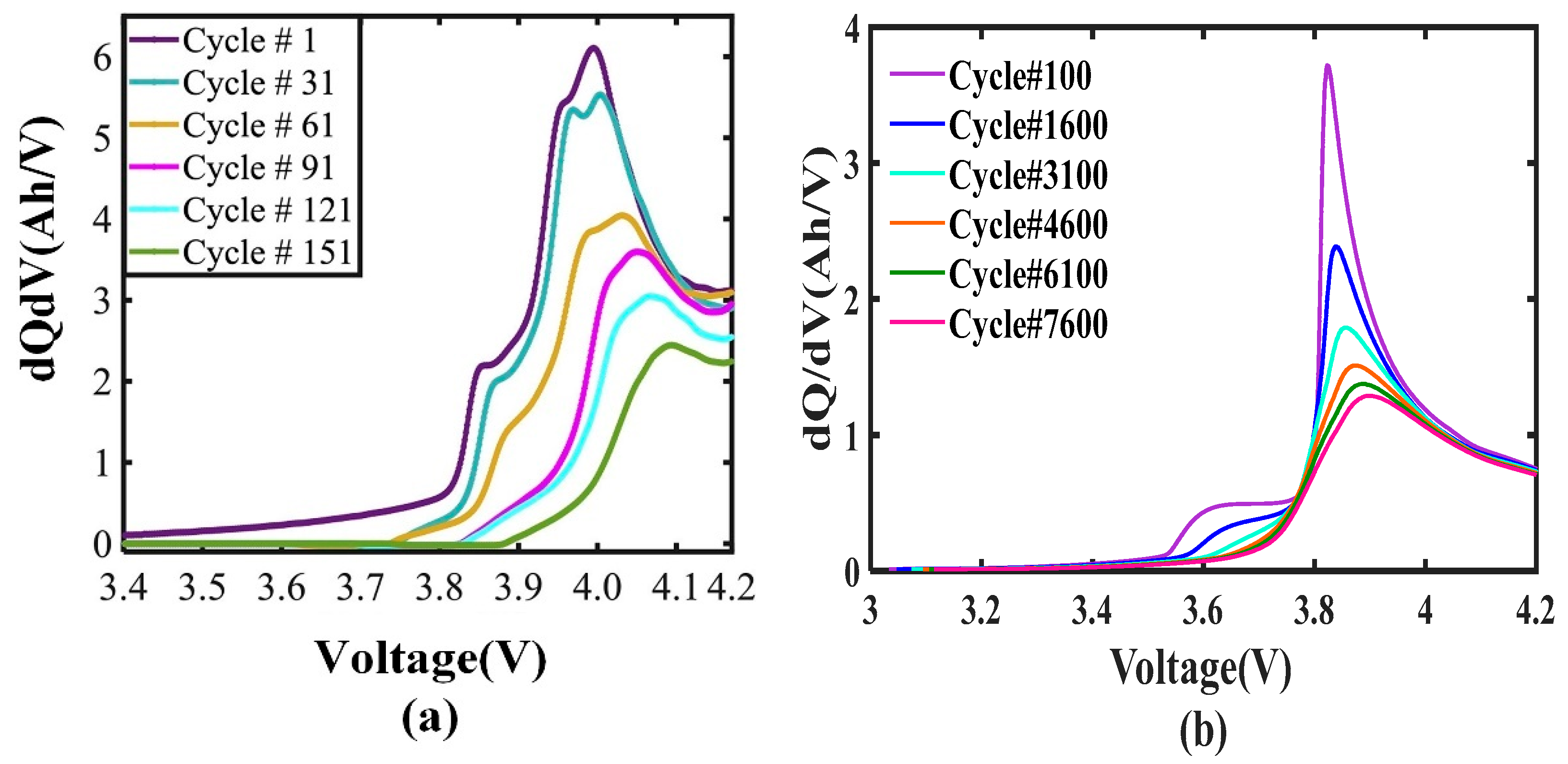
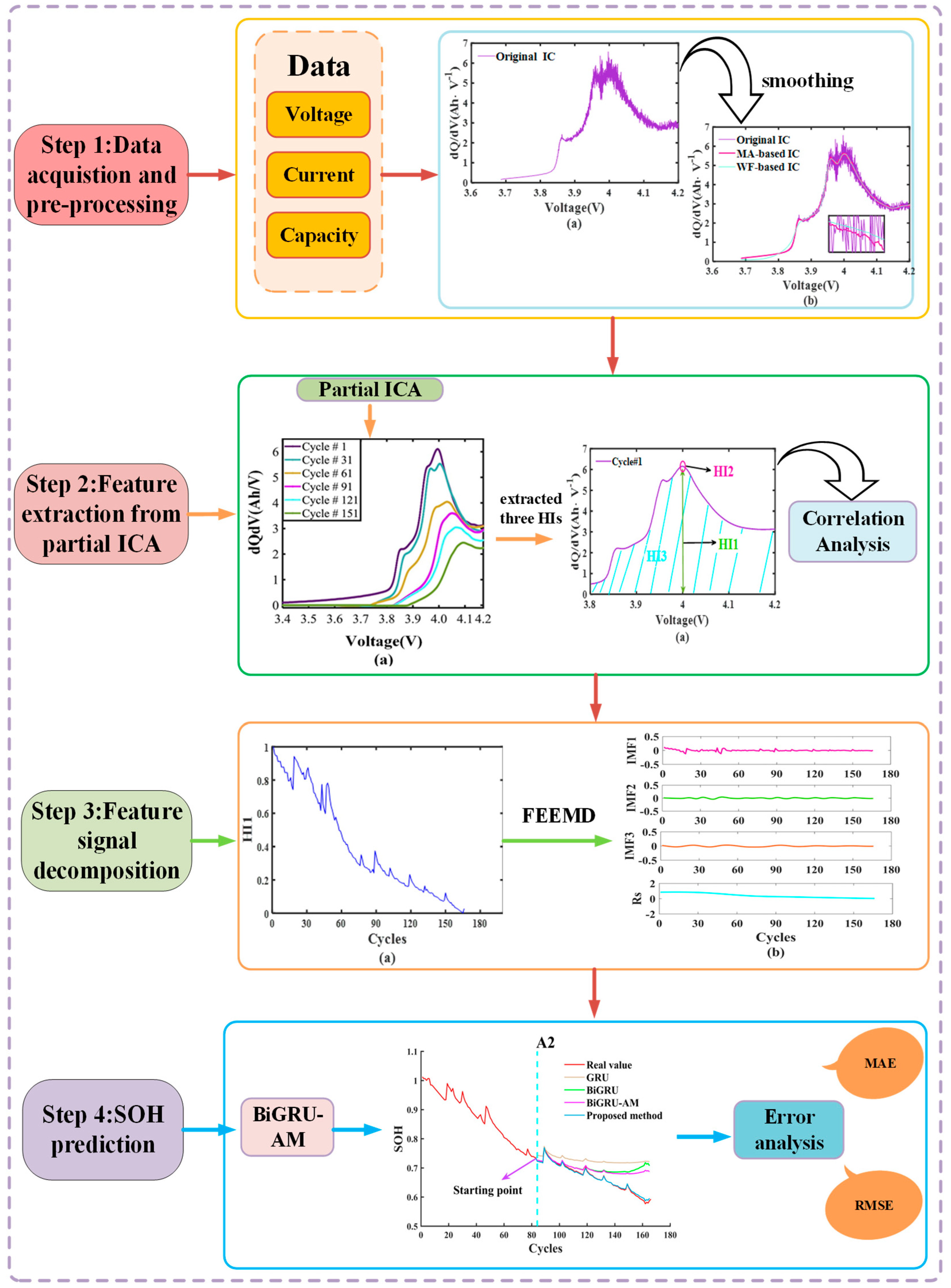
2.1. Incremental Capacity Curve Analysis and Smoothing Technique

In view of the unpredictable and uncontrollable service conditions of batteries, the charging process is an effective way to study battery degradation. IC curves and the ICA technique are widely considered mainstream methods for modeling and predicting battery health. Therefore, the battery capacity $Q$ and voltage $V$ can be shown as follows:

$$Q=It$$

(1)

$$V=f(Q), Q=f^{-1}(V)$$

(2)

where $t$ refers to the charging time and $I$ denotes the constant current during the charging CC stage. According to Equations (1) and (2), the IC curve can be expressed as follows:

$${(f^{-1})}^{\prime }={\displaystyle \frac{dQ}{dV}}={\displaystyle \frac{I\cdot dt}{dV}}=I\cdot {\displaystyle \frac{dt}{dV}}$$

(3)

Given that the original IC curves are highly sensitive to measurement noise (as shown in Figure 1a), extracting accurate aging features poses a significant challenge. To mitigate this issue, multiple effective filtering algorithms are utilized to denoise the curves and facilitate the extraction of meaningful aging features. Specifically, two filtering techniques—the Wiener filter (WF) and the moving average (MA) filter—are employed to preprocess the IC curves. The MA filter operates by replacing each data point with the average value of its neighboring points, thereby effectively smoothing out short-term fluctuations. The historical data are treated as a numerical sequence. The MA technique can be generally expressed as

$$y(i)={\displaystyle \frac{1}{N}}{\displaystyle \sum _{j=0}^{N-1}x(i+j)}$$

(4)

where $x(\cdot )$ denotes the input signals and $y(\cdot )$ represents the output signal. $N$ is the fixed window size of the series. In practice, the effectiveness of the MA method in filtering is largely contingent upon the chosen fixed window size, which needs to be kept within an appropriate range. However, this technique is computationally intensive and may not be suitable for large-scale datasets [31].

WF algorithm is extensively exploited in many fields, such as signal processing, which can be divided into two parts: wavelet signal decomposition and wavelet signal reconstruction. The most attractive property is the input noisy signal model can be represented as:

$$S(i)=f(i)+\epsilon \mathrm{e}(i)\hspace{1em}\hspace{1em}i=0,1,\dots n-1$$

(5)

where $S(i)$ denotes raw signals containing noise and $f(i)$ is the real signal. $\mathrm{e}(i)$ represents a noisy signal and $\epsilon$ is the signal strength.

The process of wavelet signal decomposition can be summarized as follows: ① The initial signal $S$ is decomposed into two parts after wavelet transformation, named low-frequency signal $L_1$ and high-frequency signal $H_1$, respectively. ② Perform the next decomposition on the low-frequency part. Namely, $L_1$ is performed to obtain the low-frequency signal $L_2$ and high-frequency signal $H_2$ after this decomposition. ③ Repeat the above steps and decompose the low-frequency signal after each decomposition. When the decomposition level reaches the preset number of layers, the decomposition ends. After n-layer wavelet decompositions, the expression of noisy signal $S$ can be written as:

$$S=L_n+H_1+H_2+\dots +H_n$$

(6)

where $L_n$ is the low-frequency signal close to the real signal $f(i)$ and $H_n$ is a potential noise signal. After applying wavelet decomposition to complete the hierarchical decomposition of the original signal, high-frequency noisy signals are selected through soft and hard threshold thresholds. Namely, if the high-frequency signal $H_n$ is higher than the preset threshold, the signal is discarded. The low-frequency signal $L_n$ obtained after wavelet decomposition and the high-frequency signal retained after threshold filtering can be reconstructed to complete wavelet denoising.

The original and filtered IC curves for battery A2 are shown in Figure 1 using the two filtering techniques. As depicted in Figure 1a, the original curve is characterized by substantial noise impulses, which complicate the direct extraction of useful information for battery SOH prognostics. To tackle this issue, two filtering algorithms are employed to smooth the raw IC curves, with the results illustrated in Figure 1b. When compared to the MA method, the WF algorithm exhibits enhanced capability in clearly identifying the peaks of the IC curves. Consequently, the WF-based approach is identified as an effective means of obtaining valuable information for forecasting battery health conditions in this study.

To verify the efficacy of the WF-based approach, the filtered IC curves for batteries A2 and B1 under various aging cycles are presented in Figure 2a,b. The results clearly demonstrate that the WF-based method successfully smooths the IC curves for both battery types. Despite this, directly inferring battery health conditions from the filtered IC curves still poses significant difficulties. Instead, extracting significant features from these curves is the optimal approach. Thus, feature extraction methods will be introduced in the following section.

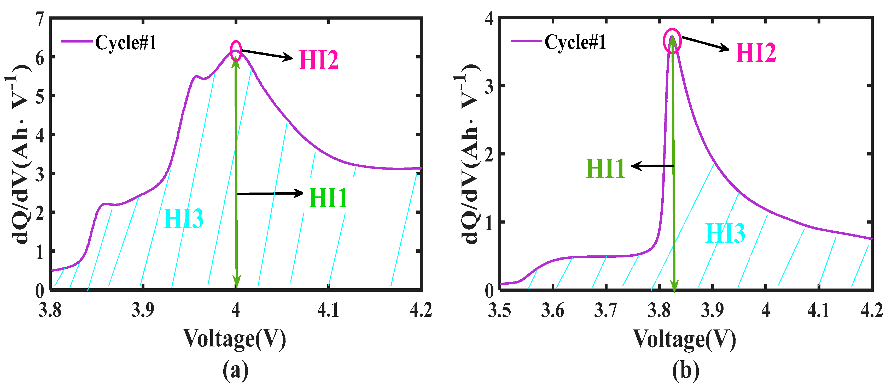
2.2. Feature Extraction

Taking the first cycle of battery A2 as an example, the voltage range of 3.8–4.2 V is identified as a critical interval for detecting degradation in battery A2, as noted in Ref. [32]. As shown in Figure 2a, the IC curves exhibit minimal changes within the 3.4–3.8 V range. In contrast, notable fluctuations are observed within the 3.8–4.2 V range, which corresponds to the primary charged capacity under varying health conditions for battery A2.

From Figure 2a,b, the entire IC curve shifts to the right as the battery ages. The peaks in the IC curves correspond to phase transitions during the electrochemical processes within lithium-ion batteries, accurately reflecting the liquid–solid transformation of cathode and anode materials during charging. The magnitude and positional shifts in these peaks indicate the dynamics of the battery’s phase transition processes, while the area under each peak is equivalent to the cumulative electrical energy during charging. As shown in Figure 3, peak height (HF1), peak position (HF2), and area under the peak (HF3) are extracted from IC curves about A2 and B1 in cycle 1 to comprehensively reflect characteristics like lithium-ion migration and chemical reaction rates in the degradation process.

2.3. The Assessment of HIs

The aging trends of HIs for A2 and B1 batteries under different aging cycles are illustrated in Figure 4. To quantitatively evaluate the rationality of the selected HIs, the Pearson’s correlation coefficient $r_p$ is utilized to evaluate the strength of the relationship between HIs and capacity in

Table 1. Results of correlation analysis.

Battery ID	${\mathit{r}}_{\mathit{p}}$ Between HI1 and Capacity	${\mathit{r}}_{\mathit{p}}$ Between HI2 and Capacity	${\mathit{r}}_{\mathit{p}}$ Between HI3 and Capacity
A1	0.9906	−0.9496	0.9981
A2	0.9955	−0.9606	0.9950
A3	0.9748	−0.9521	0.9871
B1	0.9647	−0.9776	0.9946
B2	0.9541	−0.9785	0.9948
B3	0.9689	−0.9842	0.9954

.

$$r_p={\displaystyle \frac{{\displaystyle \sum (X-\overline{X})(Y-\overline{Y})}}{\sqrt{{\displaystyle \sum {(X-\overline{X})}^2}}\sqrt{{\displaystyle \sum {(Y-\overline{Y})}^2}}}}$$

(7)

Typically, the correlation coefficient falls within the range of −1 to 1, with values closer to 1 or −1, indicating a stronger relationship between the variables. A coefficient with an absolute value above 0.8 is often considered to signify a strong correlation, while a value below 0.5 is deemed to represent a weak one. As indicated in Table 1, the maximum value of $r_p$ in HI2 is −0.9496, indicating a strong negative correlation with capacity. Whereas, in HI1 and HI3 the minimum value of $r_p$ is 0.9541 and 0.9871, respectively, which implies a strong positive correlation between HI1, HI3, and capacity.

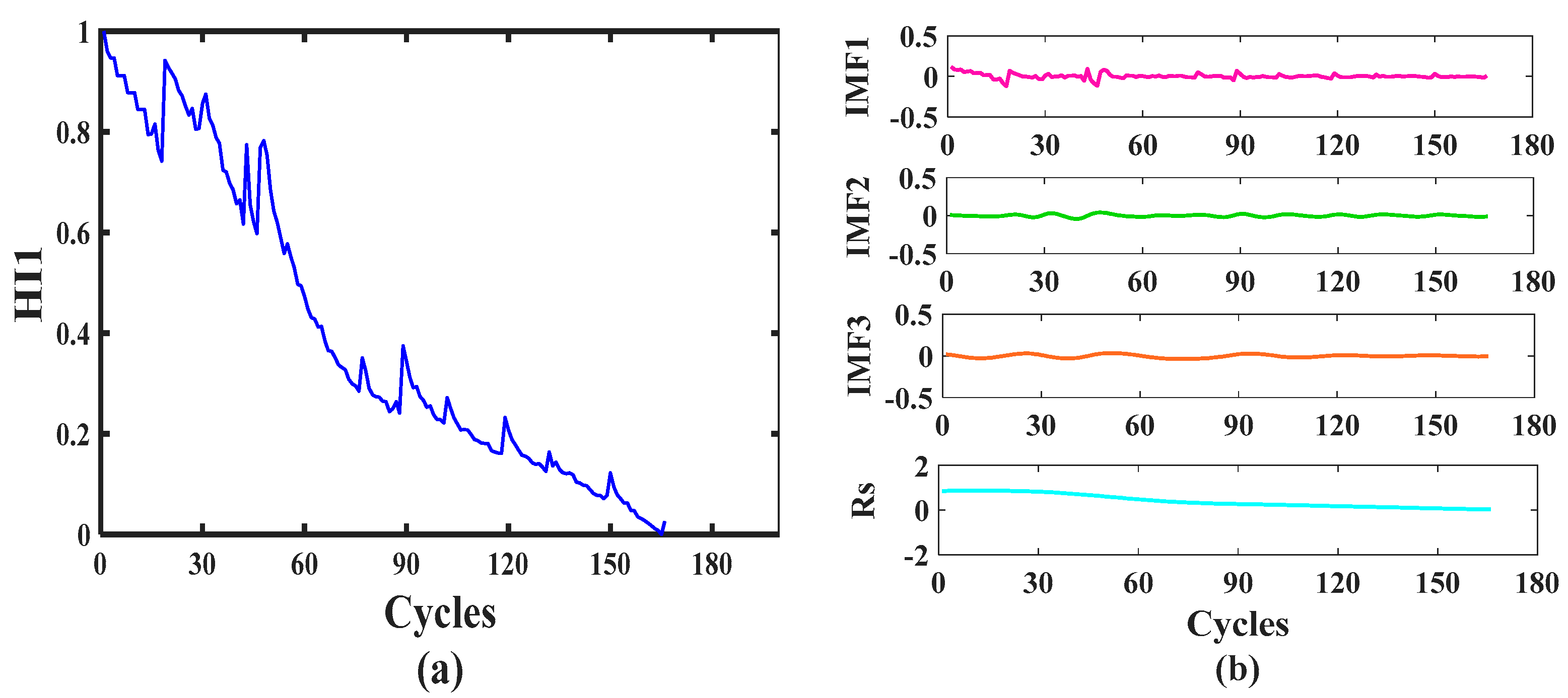
2.4. Feature Signal Decomposition

EEMD and CEEMD enhance the uniformity of the raw signal’s pole distribution by introducing white noise and overlapping anomalous signals. This process helps to mitigate or eliminate mode aliasing in EMD. However, due to the limited number of iterations, the resulting sub-layers may not strictly meet the criteria for intrinsic mode functions (IMFs). Thus, they may not be considered true IMFs. From a practical perspective, compromising the precision of sub-layers for enhanced decomposition adaptability is not ideal, as it may undermine the physical significance of the components’ instantaneous frequency [32,33]. Conversely, FEEMD seeks to maintain decomposition adaptability while preserving the physical meaning of the components.

In reality, during the decomposition of an abnormal signal, it is unnecessary to perform the full EMD on the noise that has been added. It is sufficient to ensure that the decomposition is comprehensive for the noise signal alone. Addressing this challenge, an improved version of EMD and CEEMD is introduced, known as FEEMD.

2.4.1. Box-Counting Dimension

Fractal dimension, a concept rooted in geometry, quantifies the level of chaos and intricacy within a geometric system across various scales [34]. It thereby facilitates the quantitative assessment of a signal’s randomness and irregularity.

The box-counting method is a prevalent technique for calculating fractal dimensions. In this context, the Hurst index serves as a pivotal parameter. The correlation between the fractal dimension D and the Hurst index H is described in [35].

$$D=2-H$$

(8)

As shown in Figure 5, when a specific time interval $\Delta t$ is selected, $\left|f(t_i+\Delta t)-f(t_i)\right|$ denotes the degree of volatility of the corresponding time series, $N(\Delta t)$ represents the rectangle’s coverage degree with respect to $\Delta t$.

Here, $H$ can be formulated by Equation (9):

$$H=\underset{\Delta t\to 0}{lim}{\displaystyle \frac{lgN(\Delta t)}{\Delta t}}={\displaystyle \frac{N(\Delta t)/\Delta t^2}{lg(1/\Delta t)}}$$

(9)

$$N(\Delta t)={\displaystyle \sum _{i=0}^{n-1}\left|f(t_i+\Delta t)-f(t_i)\right|}/\Delta t$$

(10)

Additionally, it can be expressed as Equation (11):

$$D=\underset{\Delta t\to 0}{lim}(2-{\displaystyle \frac{lgN(\Delta t)}{\Delta t}})=\underset{\Delta t\to 0}{lim}{\displaystyle \frac{lgN(\Delta t)/\Delta t^2}{lg(1/\Delta t)}}$$

(11)

A larger value of the box-counting dimension represents greater irregularity and complexity of the sequence; conversely, a smaller value represents less complexity and relative regularity of the time series. Since the box-counting dimension has the advantage of reflecting the randomness of the time series, it is utilized to detect and delete abnormal signals in the battery feature decline sequence.

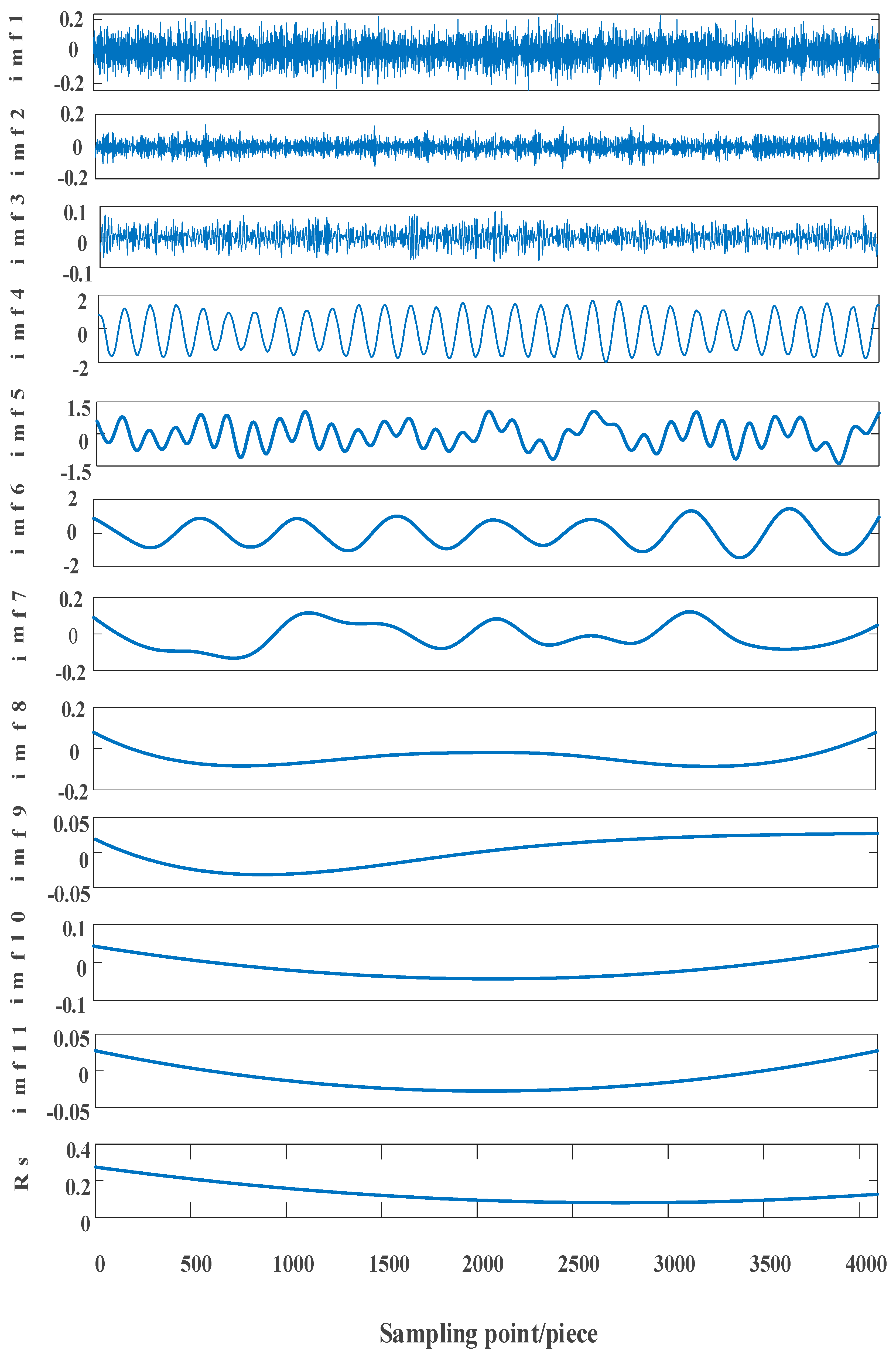
2.4.2. The Principle of FEEMD Algorithm

Taking a set of non-stationary feature signal $S(t)$ as an example, the procedures of the FEEMD algorithm can be presented in the following three steps:

(1) Within the original battery degradation feature signal $S(t)$, paired white Gaussian noise signals $n_i(t)$ and $-n_{\mathrm{i}}(t)$ are separately added. Hence, two novel battery degradation feature signals $s_i^{+}(t)$ and $s_i^{-}(t)$ are created, which can be expressed as:

$$S_{\mathrm{i}}^{+}(t)=S(t)+a_i{n}_i(t)$$

(12)

$$S_{\mathrm{i}}^{-}(t)=S(t)-a_i{n}_i(t)$$

(13)

Among them: $a_i$ represent the amplitude of the added white noise, $i=1,2,\dots ,Ne$. $Ne$ means the logarithm of them, of which $Ne$ is usually no more than 100. Then, EMD on $S_i^{+}(t)$ and $S_i^{-}(t)$ are performed, respectively, and the first-order IMF1 sequence $\left\{I_{\mathrm{i}1}^{+}(t)\right\}$ and $\left\{I_{\mathrm{i}1}^{-}\left(t\right)\right\}$ $(i=1,2,\dots ,Ne)$ can be obtained.

$$I_1(t)={\displaystyle \frac{1}{2N}}{\displaystyle \sum _{\mathrm{i}=1}^{Ne}\left[I_{\mathrm{i}1}^{+}(t)+I_{\mathrm{i}1}^{-}(t)\right]}$$

(14)

To identify whether $I_1(t)$ is abnormal: If the box-counting dimension of the signal exceeds a certain threshold, it is deemed abnormal. Otherwise, it is considered approximately stable. Through numerous simulations, a threshold of 1.22 has been found to be optimal.

(2) If the signal $I_1(t)$ is identified as abnormal, step (1) will be continuously carried out until the $I_P(t)$ becomes a stationary signal.

(3) The aforementioned decomposed components are removed from $S(t)$, which means that:

$$r(t)=S(t)-{\displaystyle \sum _{j=1}^{p-1}{I}_j}(t)$$

(15)

(4) After isolating the abnormal signals, the remaining signals (denoted as $r(t)$) are further processed using EMD to decompose them into IMFs and Rs. This marks the completion of the FEEMD process.

2.4.3. Decomposition Performance of FEEMD

To demonstrate the superior performance of FEEMD, a simulation signal is employed for validation purposes:

$$s(t)=2\sin (60\pi t+\pi /2)+(t+1)\sin (16\pi t+\pi /3)+n(t)$$

(16)

Among them: $t=1/4096:1/4096:1$, the sampling time is 1 s, the sampling frequency is 4096 Hz, and the number of sampling points is 4096. $n(t)$ is a white Gaussian noise signal of 20 db. Figure 6, Figure 7 and Figure 8 illustrate the decomposition results of $s(t)$ decomposed by EMD, CEEMD, and FEEMD, correspondingly.

The results depicted in Figure 6, Figure 7 and Figure 8 demonstrate that, compared to EMD and CEEMD, the FEEMD technique achieves more thorough decomposition of high-frequency sub-layers, resulting in smoother waveform components. Remarkably, the high–frequency component (imf1) exhibits symmetric oscillations and prominent periodicity.

Initially, the presence of noise leads to significant mode aliasing in EMD, as indicated by the red circle in Figure 6. While CEEMD mitigates this issue to some extent, the decomposition results still contain spurious and interfering sub-components (e.g., imf5–imf11). In contrast, FEEMD effectively eliminates these false components, resulting in a cleaner decomposition.

To validate the generalization capability of the FEEMD method, 1000 sets of signals were randomly selected for analysis. The decomposition performance was evaluated using three key indicators: completeness, orthogonality, and computational time. The Index of Orthogonality (IO) measures the orthogonal relationship between sub-sequences, thereby indicating the degree of mode mixing. In this study, the Index of Overall Orthogonality (IOO) is employed. Specifically, the differences between the decomposed sub-layers and the raw signal are used to quantify the extent of mode mixing. Typically, a larger value of the IOO indicates more severe mode mixing. The three metrics can be expressed as follows:

$$I{O}_{i,k}={\displaystyle \sum _{t=0}^z\frac{c_i(t)c_k(t)}{c_i(t)+c_k(t)}}$$

(17)

$$IOO={\displaystyle \frac{1}{A(A-1)}}{\displaystyle \sum _{i,k=0}^{A}I}{O}_{i,k},i\ne k$$

(18)

In Equations (17) and (18), $A$ is the number of decomposed components. $c(t)$ indicates the decomposed sub-components. The results obtained by averaging the three evaluation indices across 1000 sets of simulated signals are presented in

Table 2. Evaluation indicators for the decomposition of 1000 sets of random signals.

Time-Frequency Algorithms	$\mathit{I}\mathit{O}\mathit{O}$	$\mathit{T}\mathit{i}\mathit{m}\mathit{e}$/s
EMD	0.2762	6.847
CEEMD	0.1377	19.288
FEEMD	0.0574	10.280

.

As clearly shown in Table 2, in terms of the IOO, FEEMD exhibits the lowest value, indicating that it has the least mode mixing compared to the other three techniques. Regarding computational time, although FEEMD is not as fast as EMD, its processing time remains within an acceptable range. Based on the above analysis, we can confidently conclude that FEEMD demonstrates significant advantages over the other three time-frequency decomposition methods.

2.4.4. Feature Decomposition

Taking the normalized HI1 of A2 as an example, Figure 9a,b show the original normalized HI1 and the decomposed normalized HI1 by FEEMD, respectively. It can be easily found that the FEEMD can decrease nonlinearity and fluctuations in the normalized HI1 to a great extent.

2.5. Forecasting Method

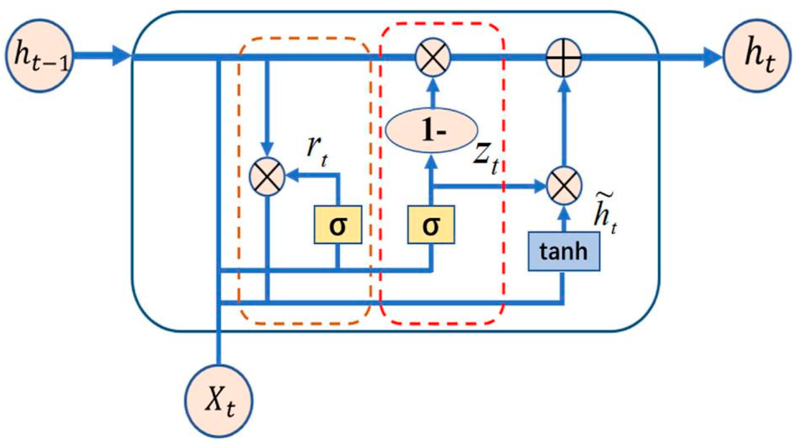
2.5.1. Bidirectional Gated Recurrent Unit (BiGRU)

BiGRU is capable of detecting long-term dependencies and extracting semantic details from the original data. In the model, the GRU method’s directional property is strengthened. This is achieved by incorporating a second layer, which links two hidden layers running in opposite directions to a common output layer. As shown in Figure 10, $X_t$ and $h_t$ denote the input and output at the time $t$, respectively. $r_t$ and $z_t$ are reset gate and update gate, respectively. The reset gate combines historical data with the current input, and the update gate regulates the degree to which historical information is preserved. The crucial parameters are in the following manner:

$$z_t=\sigma ({\mathrm{w}}_z[h_{t-1},x_t]+b_z)$$

(19)

$$r_t=\sigma ({\mathrm{w}}_{\mathrm{r}}[h_{t-1},x_t]+b_r)$$

(20)

$$\widetilde{{\mathrm{h}}_t}=\tanh ({\mathrm{w}}_h[r_t{h}_{t-1},x_t]+b_h)$$

(21)

$$h_t=(1-z_t)h_{t-1}+z_t\widetilde{h_t}$$

(22)

where $\sigma$ and $tanh$ denote various activation functions, $\widetilde{h_t}$ represents the information newly generated through the update gate. $w$ represents the weight coefficient and $b$ is the bias in the corresponding layer.

The architecture of the BiGRU neural network can be observed in Figure 11. While the forward propagation in BiGRU is comparable to that of the GRU neural network, the key difference lies in the time series data flow: BiGRU processes the input sequence in reverse through its two hidden layers. The hidden states $Y_t$ are obtained through the concatenation of these two outputs.

$$Y_t=H_t^f\oplus H_t^b$$

(23)

2.5.2. Bidirectional Gated Recurrent Unit with Attention Mechanism (BiGRU-AM)

The AM mimics the human brain’s ability to allocate attention, effectively focusing on critical information while minimizing attention to irrelevant details, thereby enhancing the model’s computational efficiency. The AM’s structure is presented in Figure 12, in which $x_t$ denotes the input, $h_t$ corresponds to the hidden layer output obtained by BiGRU, $a_t$ represents the attention distribution of the BiGRU hidden layer output by the AM, and $y$ is the output with the introduction of the AM.

3. Architecture of the Proposed Framework

Given the ambiguity and stochastic nature of the degradation time series of LIBs, a solitary framework falls short of attaining desirable prediction results. Hence, in this investigation, a hybrid prediction configuration that makes use of IC curve filtering, feature extraction, feature signal decomposition, and an aging model is exhibited. As presented in Figure 13, the subsequent content will elaborate on the details of the proposed hybrid model:

Stage I: Data acquisition and pre-processing. Leveraging historical monitoring data, the IC curve is derived from voltage and current measurements to discern the degradation trend. Subsequently, the WF algorithm is utilized to mitigate noise in the raw IC curves;

Stage Ⅱ: Feature extraction from partial ICA. The important region of IC curves is chosen as the research object of feature extraction. Then, battery features, including peak height, peak position, and the regional area under the peak value, are extracted in this research. Subsequently, the correlation coefficient is utilized to evaluate the extent of the relationship between the features that have been extracted and the loss of battery capacity;

Stage Ⅲ: Feature signal decomposition. In order to decrease the big fluctuations and nonlinearity in extracted HFs, FEEMD is proposed and utilized to decompose the high-relation degree features in stage Ⅱ to obtain several sub-layers;

Stage Ⅳ: SOH prediction. Considering the nonlinear connection between the sub-layers decomposed by FEEMD and the SOH, a two-layer deep-learning model founded on the BiGRU-AM is devised to forecast the SOH. Eventually, two datasets are utilized to verify the accuracy and robustness of the proposed model.

4. Experimental Results and Discussion

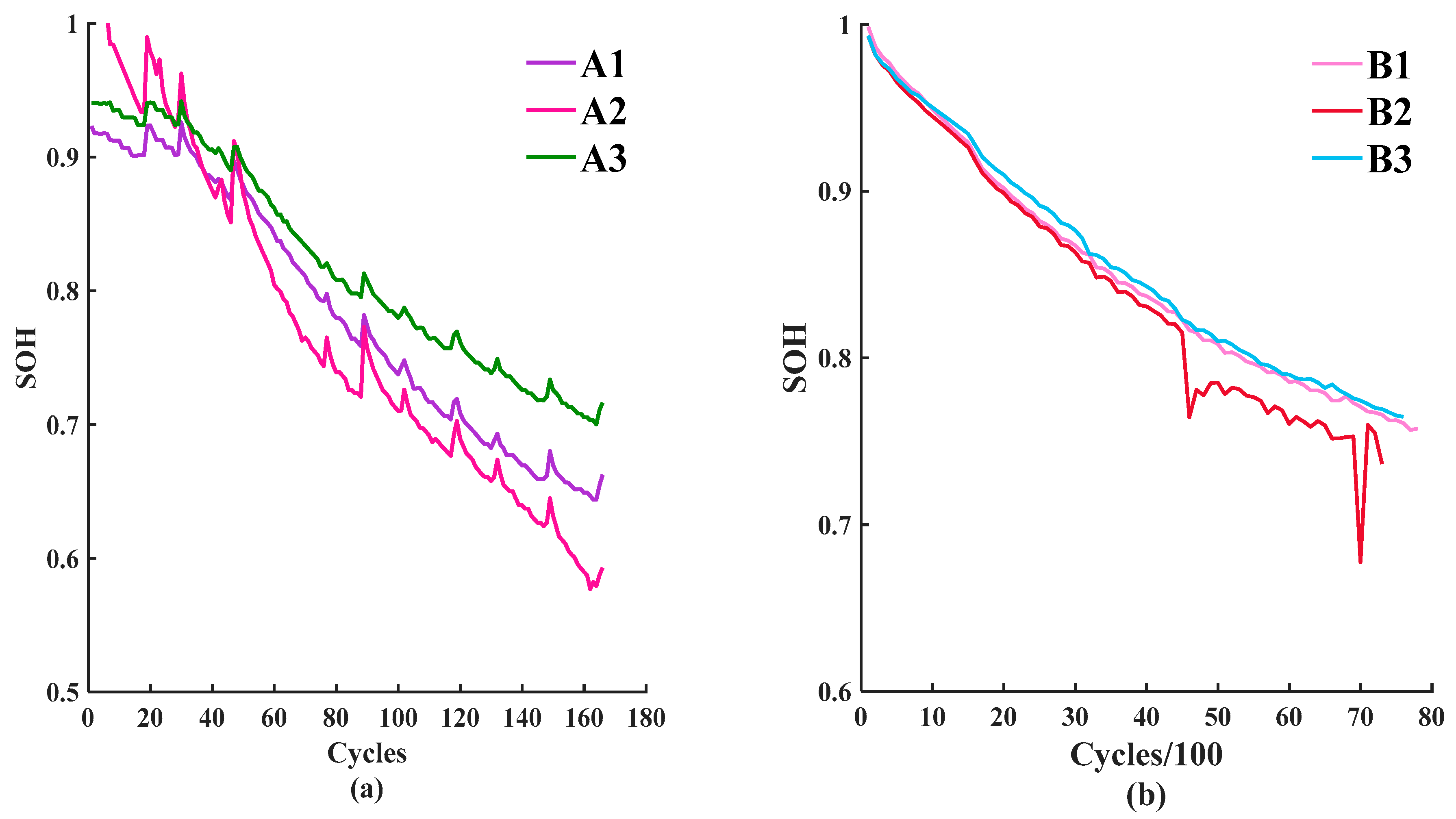
4.1. Datasets Description

In this study, two publicly available lithium-ion battery degradation datasets are utilized to assess the performance of the proposed framework. One dataset is sourced from the NASA Ames Prognostics Center of Excellence and was measured using lithium-ion 18,650 batteries. Three cells, namely B005, B006, and B007, are chosen as the research subjects. In this paper, they are, respectively, referred to as A1, A2, and A3.

To further boost the robustness of the proposed model, the Oxford dataset is chosen as an additional case study within this research. Each of these cells has a nominal capacity of 740 mAh and was tested within a hot chamber maintained at 40 °C. The cells underwent the ARTEMIS urban driving cycle for discharging, followed by being charged with a 2C constant current to complete each cycle. For this study, three cells (referred to as cell1, cell2, and cell3) are chosen and designated as B1, B2, and B3, respectively, in the subsequent analysis.

The detailed experimental information for the six battery cells in the two datasets is displayed in

Table 3. The detailed experimental information in the two datasets.

Dataset	Form Factor	Cell Anode	Cell Cathode	Charge Conditions	Discharge Conditions	Nominal Capacity	Nominal Voltage	Upper Cut-Off Voltage	Lower Cut-Off Voltage
NASA	18,650	Graphite	LiCoO2/LiNiCoAlO2	CC-CV	1C	2 Ah	-	4.2 V	2.7 V, 2.5 V, 2.2 V, 2.5 V
Oxford	Pouch	Graphite	LiCoO2/LiNiMnCoO2	2C	Artemis urban drive cycle	0.74 Ah	3.7 V	4.2 V	2.7 V

. The SOH decline curves of the six batteries with the increase in the number of cycles are provided in Figure 14a,b. In Figure 14a (NASA dataset), the blue curve represents cell A1, the red curve corresponds to cell A2, and the green curve denotes cell A3. For the Oxford dataset in Figure 14b, the cyan curve indicates cell B1, the magenta curve represents cell B2, and the yellow curve corresponds to cell B3. Each curve clearly illustrates the distinct degradation trajectories of different battery cells, providing a visual basis for evaluating the proposed model’s performance across diverse datasets.

4.2. Hyperparameters Setting

The BiGRU-AM network learns from dynamic feature vectors and employs a weight-sharing mechanism to drive shared network parameters in learning common features. It thoroughly explores the changing patterns of battery health status and ultimately achieves dynamic modeling of both input and output data. The initial learning rate is set to 0.001, and the training is conducted for 300 epochs. Each step corresponds to two hidden layers: one processes data from front to back, and the other processes data from back to front. The number of nodes in the first hidden layer ranges from 10 to 30, while the number of nodes in the second hidden layer ranges from 10 to 40. The batch size ranges from 8 to 32.

The six batteries are split into a training set and a testing set, each comprising 50% of the total dataset. During the training process, the model was trained for 500 epochs. In each iteration, a batch of data was randomly selected from the training set. The input data for the model consisted of the decomposed HFs obtained from the FEEMD process. These features were first normalized to a range of [0, 1] to ensure that each feature had an equal impact on the model training.

All the experiments were conducted on the Matlab 2024a platform. The model’s trainable parameters are updated via the Adam optimizer, which has been demonstrated to be an efficient and robust optimizer for shield parameter prediction. The computational platform is equipped with an NVIDIA RTX 2080 Ti GPU and Intel 13,700 K CPU.

4.3. Evaluation Benchmarks

The following indexes are adopted as evaluation criteria, which contain root mean square error ($RMSE$) and mean absolute error ($MAE$), denoted as follows:

$$RMSE=\sqrt{{\displaystyle \frac{1}{m}}{\displaystyle \sum _{i=1}^m{(y_i-\widehat{y_i})}^2}}$$

(24)

$$MAE={\displaystyle \frac{1}{m}}{\displaystyle \sum _{i=1}^m\left|y_i-\widehat{y_i}\right|}$$

(25)

where $\widehat{y_i}$ denotes the predicted SOH, $y_i$ represents the real SOH, $m$ is the number of testing cycles.

4.4. Comparative Experiments

4.4.1. Comparative Experiments I

To comprehensively evaluate the prediction performance of the proposed hybrid model, three distinct single models (namely, GRU, BiGRU, and BiGRU-AM) are chosen for comparative analysis in Experiment I. The experiments are conducted on the Matlab 2024a platform. The SOH prediction results for these models are illustrated in Figure 15, while the corresponding MAE and RMSE values are summarized in

Table 4. MAE and RMSE of SOH prediction results of four models.

Battery ID	MAE (%)				RMSE (%)
	GRU	BiGRU	BiGRU-AM	Proposed	GRU	BiGRU	BiGRU-AM	Proposed
A1	4.67	3.18	2.70	0.20	6.97	4.88	3.31	0.31
A2	3.59	2.62	1.97	0.36	5.73	3.84	2.35	0.39
A3	6.96	4.84	3.66	0.28	9.39	6.34	3.89	0.48
B1	1.27	0.83	0.66	0.59	1.83	1.14	0.86	0.55
B2	1.16	0.75	0.53	0.38	1.77	1.05	0.73	0.43
B3	0.94	0.80	0.66	0.40	1.53	1.25	0.94	0.44

.

In Figure 15, the red lines indicate the actual SOH, while the khaki, green, and magenta lines correspond to the predicted SOH values from the GRU, BiGRU, and BiGRU-AM models, respectively. Additionally, the blue lines represent the predictions from the proposed hybrid method. It is evident that the khaki curves deviate significantly from the true values, suggesting that the GRU model performs the least accurately among the four methods. In contrast, the blue curves closely follow the trend of the red lines, indicating that the proposed model in this study achieves the highest prediction accuracy and its results are the closest to the actual SOH values. Moreover, as shown in Table 4, it is evident that the error metrics of the proposed method are lower than those of the other comparative models when applied to six LIBs. For example, in cell A3, the MAE of the proposed approach is reduced by 6.68%, 4.56%, and 3.38% compared to the other models. Similarly, the RMSE in cell A3 can be decreased by 8.91%, 5.86%, and 3.41%, respectively. These findings are consistent across other cells as well, indicating the superiority of the proposed technique. Moreover, a comparison between the evaluation results of the proposed model and those of the BiGRU-AM model demonstrates that the decomposition method significantly enhances forecasting accuracy. This finding underscores the effectiveness of the decomposition technique in mitigating the nonlinearity of features. The irregular fluctuations of the features significantly complicate prognostic tasks. However, the decomposition method effectively addresses this challenge by breaking down the raw data into multiple subseries, thereby mitigating the randomness of the features. As a result, the above results demonstrate that the prediction accuracy of the proposed hybrid method is better than the single model. Consequently, the method we have proposed is more advantageous in uncovering the degradation trend of the SOH. Moreover, it can effectively improve prediction accuracy.

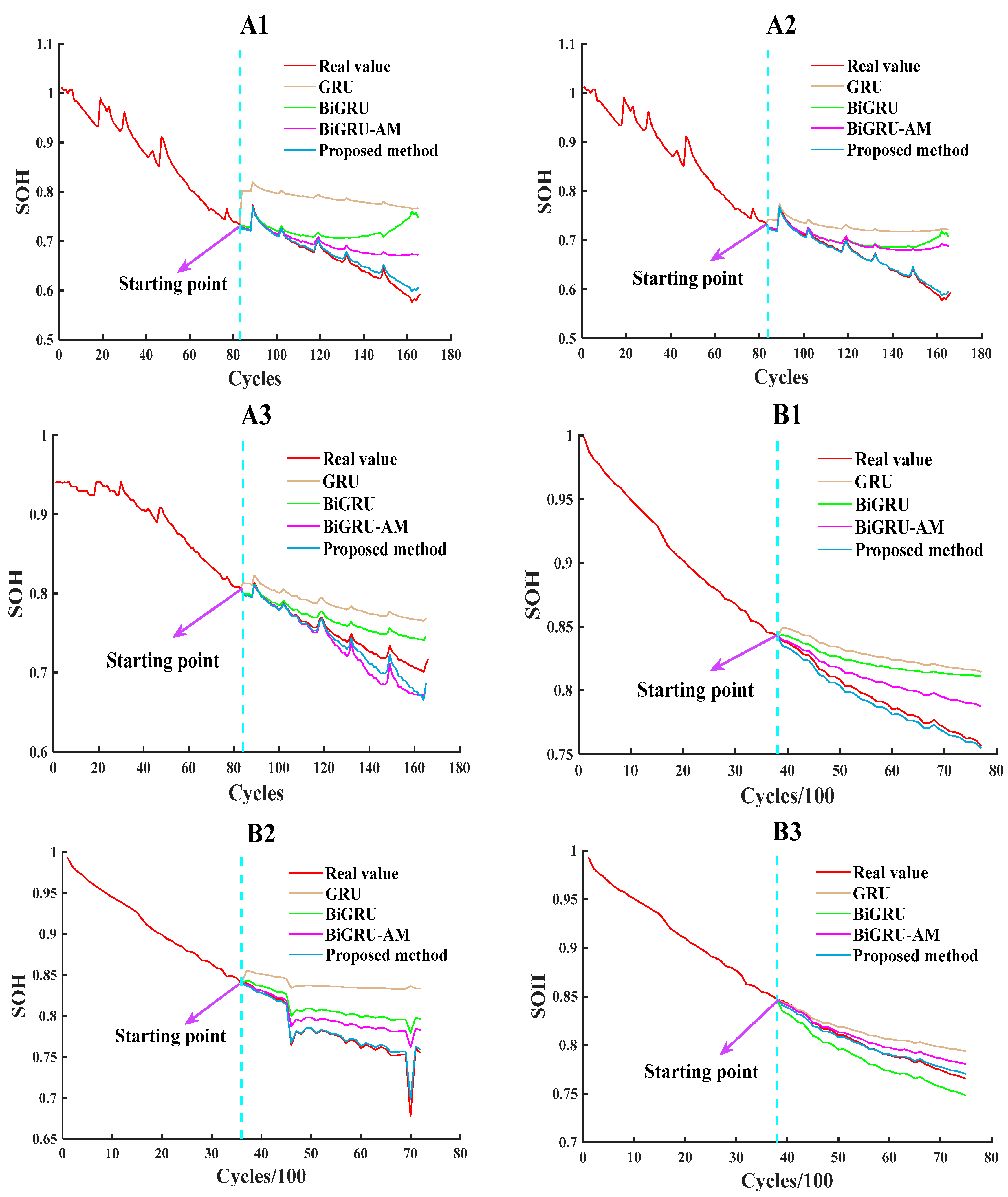
4.4.2. Comparative Experiments II

To further illustrate the prediction capabilities of the proposed hybrid model, three model comparisons (EMD-BiGRU-AM, CEEMD-BiGRU-AM, and the proposed method) are conducted in Experiment II. These comparisons highlight the significance of the FEEMD approach by contrasting it with EMD-BiGRU-AM and CEEMD-BiGRU-AM. Figure 16 presents the MAE and RMSE of the three models, respectively. Based on Figure 16, the detailed comparative discussions and results are summarized in the following:

According to Figure 16, the khaki lines, green lines, and magenta lines represent the predicted SOH concerning GRU, BiGRU, BiGRU-AM, and the proposed method, respectively. From Figure 16a, the MAE values for the proposed method are obviously less than the other two models (EMD-BiGRU-AM and CEEMD-BiGRU-AM), which are both within 0.7% while the others are all beyond 1%. Figure 16b presents the RMSE results for a total of six batteries. These results offer a quantitative analysis of the prediction accuracy. As depicted in the figure, the RMSE values for five out of the six cells are below 0.5%. Only cell A3 has a slightly higher RMSE value. Through these two error analysis methods, it is evident that the proposed algorithm consistently yields the most accurate prognostic results across all cases compared to the other models involved. These findings indicate that FEEMD outperforms EMD and CEEMD in terms of prediction accuracy. Thus, FEEMD is more effective in identifying the SOH degradation trend and enhancing prediction accuracy.

4.4.3. Comparative Experiments III

In this section, for the purpose of further verifying the evaluation performance of the proposed technique, the current state of the art of SOH estimation models in other newly published studies are also compared with the proposed method for six batteries, and the comparison results can be demonstrated in Table 5 and Table 6.

As shown in Table 5 and Table 6, the proposed method achieves the lowest MAE and RMSE values across all six battery cells. For example, in cell A3, the MAE of 0.28% and RMSE of 0.48% significantly outperform the Gaussian process regression (GPR)-based method in [35] (MAE: 0.357%, RMSE: 0.522%) and the improved LSTM in [36] (MAE: 0.4163%, RMSE: 0.5338%). This superiority is attributed to the synergistic effect of FEEMD’s noise mitigation and the BiGRU-AM’s ability to prioritize critical temporal features.

Table 5. Comparison prediction results for A1, A2, and A3.

Error	MAE (%)				RMSE (%)
Battery ID	[37]	[38]	[39]	Proposed	[37]	[38]	[39]	Proposed
A1	0.279	0.3287	0.92	0.20	0.349	0.4077	1.27	0.31
A2	0.400	0.7219	1.10	0.36	0.479	0.9587	1.53	0.39
A3	0.357	0.4163	1.34	0.28	0.522	0.5338	1.62	0.48

Table 5. Comparison prediction results for A1, A2, and A3.

Error	MAE (%)				RMSE (%)
Battery ID	[37]	[38]	[39]	Proposed	[37]	[38]	[39]	Proposed
A1	0.279	0.3287	0.92	0.20	0.349	0.4077	1.27	0.31
A2	0.400	0.7219	1.10	0.36	0.479	0.9587	1.53	0.39
A3	0.357	0.4163	1.34	0.28	0.522	0.5338	1.62	0.48

Table 6. Comparison prediction results for B1, B2, and B3.

Error	MAE (%)			RMSE (%)
Battery ID	[40]	[41]	Proposed	[40]	[41]	Proposed
B1	0.753	0.64	0.59	0.915	0.70	0.55
B2	1.637	0.44	0.38	1.834	0.79	0.43
B3	1.288	0.46	0.40	1.564	0.57	0.44

Table 6. Comparison prediction results for B1, B2, and B3.

Error	MAE (%)			RMSE (%)
Battery ID	[40]	[41]	Proposed	[40]	[41]	Proposed
B1	0.753	0.64	0.59	0.915	0.70	0.55
B2	1.637	0.44	0.38	1.834	0.79	0.43
B3	1.288	0.46	0.40	1.564	0.57	0.44

The results highlight the framework’s versatility across different battery chemistries and degradation profiles. For instance, in the Oxford dataset (B1–B3), which involves pouch cells with dynamic discharge cycles, the proposed method maintains MAE below 0.59% and RMSE below 0.55%, outperforming the differential thermal capacity-based approach in [38] (MAE: 0.753%, RMSE: 0.915%). This robustness is critical for real-world applications, where batteries are subject to non-uniform operational conditions.

Table 5 and Table 6 indicate that the proposed method yields significantly lower MAE and RMSE values for six cells compared to other newly published methods. Based on the experimental results, the proposed methodology—comprising the extraction of optimal health indicators (HIs), their decomposition through FEEMD, and the utilization of a BiGRU-AM network to establish nonlinear relationships between HIs and SOH—demonstrates robust feasibility for achieving accurate prognoses of lithium-ion battery health states. This integrated approach offers a reliable and innovative framework for translating experimental insights into practical battery management applications. Through comparisons with the prediction methods proposed in other documents, the credibility and effectiveness of the proposed approach are further validated.

4.4.4. Error Source Analysis and Robustness Evaluation

There are several potential error sources in the proposed model. Firstly, the feature extraction process from the IC curves might introduce errors. Although PICA and the selection of features like peak height, peak position, and peak area are effective in general, the accuracy of these features can be affected by noise in the measurement data, even after WF. Residual noise might still distort the true characteristics of the battery degradation, leading to inaccurate feature values. Additionally, the assumption that these features comprehensively represent the battery’s health state might not hold true in all cases. There could be other hidden factors in the battery’s electrochemical processes that are not captured by these features, resulting in incomplete information for the model.

Secondly, the FEEMD decomposition has its own limitations. Although it effectively reduces the nonlinearity and fluctuations of the features, the decomposition process is based on certain mathematical assumptions. In some cases, the decomposition might not accurately reflect the true physical meaning of the sub-layers, especially when dealing with complex electrochemical signals. This could lead to errors in the subsequent prediction by the BiGRU-AM model.

Finally, the BiGRU-AM model itself is also a source of error. The hyperparameters of the model, such as the number of hidden units, learning rate, and batch size, were determined through a certain tuning process. However, these values might not be optimal for all battery datasets and operational conditions. Sub-optimal hyperparameters can lead to issues like overfitting or underfitting, which will degrade the model’s prediction accuracy.

To evaluate the performance of the proposed model in predicting battery SOH, three sets of comparative experiments were designed and executed. The effectiveness of the method was rigorously assessed using two extensively recognized error analysis metrics. The results reveal that the proposed FEEMD-based approach achieved remarkable accuracy, with the maximum values of MAE and RMSE reaching only 0.59% and 0.55%, respectively. These statistics significantly outperform those of the benchmark models, underscoring the superiority of the proposed method. The exceptional performance of the model not only validates its effectiveness but also provides a robust and dependable basis for the accurate health prognosis of lithium-ion batteries, which is crucial for ensuring the safety and efficiency of battery-powered systems.

5. Conclusions and Future Work

5.1. Conclusions

LIBs have become integral in numerous critical applications within the electronics sector. Ensuring their safety and reliability necessitates the development of precise SOH prognostics. This study introduces an innovative framework that combines PICA, feature extraction, FEEMD, and BiGRU-AM for SOH prediction. The degradation data utilized in this research were collected from six batteries across two types. The key contributions of our method are outlined below: (1) Two distinct filtering algorithms were employed to refine the battery IC curves, with the superior approach being selected for further analysis in this study. (2) Focusing on the primary battery charging region, significant health features were extracted from the PICA curves. Concurrently, a correlation analysis method was applied to quantitatively assess the relationship between these health features and the aging capacity of the batteries. (3) In order to decrease the nonlinearity and fluctuations in HFs, FEMMD is first proposed and introduced to decompose the HFs into a series of sub-layers. (4) The BiGRU-AM model, enhanced by the attention mechanism, is employed to predict the sub-layers. This mechanism allows the model to concentrate on the critical information within the sub-layers while filtering out irrelevant details. Three groups of comparative experiments are employed to predict battery SOH and to compare the performance of the proposed model. Two widely used error analysis indices are employed to assess and validate the performance of the proposed method. The highest values of the MAE and the RMSE are 0.59% and 0.55%, respectively.

5.2. Future Work

While the proposed framework demonstrates robust performance on controlled laboratory datasets, the generalization to real-world battery operations—characterized by dynamic environmental conditions, non-uniform usage profiles, and heterogeneous battery chemistries—remains a critical frontier. To address this, our future work will focus on the following directions: including extreme temperatures (e.g., −30 °C to 60 °C), dynamic loads, and varied battery chemistries (NMC, LFP). Techniques like domain-adaptive algorithms and online semi-supervised learning will enhance robustness against dataset shifts, while integrating simplified electrochemical models will improve interpretability and detect rare failure modes. Longitudinal field trials over 12 months, including real-time validation on electric bus fleets and grid-tied storage systems, aim to transform the lab-proven framework into an industrially viable solution, ensuring reliable battery management across heterogeneous operational scenarios.

References

1. Lipu, M.H.; Hannan, M.; Hussain, A.; Hoque, M.; Ker, P.J.; Saad, M.; Ayob, A. A review of state of health and remaining useful life estimation methods for lithium-ion battery in electric vehicles: Challenges and recommendations. J. Clean. Prod. 2018, 205, 115–133. [Google Scholar] [CrossRef]
2. Liu, K. Data-driven health estimation and lifetime prediction of lithium-ion batteries: A review. Renew. Sustain. Energy Rev. 2019, 113, 109254. [Google Scholar] [CrossRef]
3. Von Buelow, F.; Meisen, T. A review on methods for state of health forecasting of lithium-ion batteries applicable in real-world operational conditions. J. Energy Storage 2023, 57, 105978. [Google Scholar] [CrossRef]
4. Li, W.; Fan, Y.; Ringbeck, F.; Jöst, D.; Han, X.; Ouyang, M.; Sauer, D.U. Electrochemical model-based state estimation for lithium-ion batteries with adaptive unscented Kalman filter. J. Power Sources 2020, 476, 228534. [Google Scholar] [CrossRef]
5. Ouyang, T.; Xu, P.; Chen, J.; Lu, J.; Chen, N. An Online Prediction of Capacity and Remaining Useful Life of Lithium-Ion Batteries Based on Simultaneous Input and State Estimation Algorithm. IEEE Trans. Power Electron. 2020, 36, 8102–8113. [Google Scholar] [CrossRef]
6. Sun, Q.; Zeng, G.; Xu, X.; Li, J.; Biendicho, J.J.; Wang, S.; Tian, Y.; Ci, L.; Cabot, A. Are Sulfide-Based Solid-State Electrolytes the Best Pair for Si Anodes in Li-Ion Batteries? Adv. Energy Mater. 2024, 14, 2402048. [Google Scholar] [CrossRef]
7. Li, J.; Zeng, G.; Horta, S.; Martínez-Alanis, P.R.; Biendicho, J.J.; Ibáñez, M.; Xu, B.; Ci, L.; Cabot, A.; Sun, Q. Crystallographic Engineering in Micron-Sized SiOx Anode Material Toward Stable High-Energy-Density Lithium-Ion Batteries. ACS Nano 2025, 19, 16096–16109. [Google Scholar] [CrossRef]
8. Liu, B.; Tang, X.; Gao, F. Joint estimation of battery state-of-charge and state-of-health based on a simplified pseudo-two-dimensional model. Electrochim. Acta 2020, 344, 136098. [Google Scholar] [CrossRef]
9. Liu, C.; Wang, Y.; Chen, Z. Degradation model and cycle life prediction for lithium-ion battery used in hybrid energy storage system. Energy 2019, 166, 796–806. [Google Scholar] [CrossRef]
10. Shen, D.; Wu, L.; Kang, G.; Guan, Y.; Peng, Z. A novel online method for predicting the remaining useful life of lithium-ion batteries considering random variable discharge current. Energy 2021, 218, 119490. [Google Scholar] [CrossRef]
11. Shi, E.; Xia, F.; Peng, D.; Li, L.; Wang, X.; Yu, B. State-of-health estimation for lithium battery in electric vehicles based on improved unscented particle filter. J. Renew. Sustain. Energy 2019, 11, 024101. [Google Scholar] [CrossRef]
12. Zheng, L.; Zhu, J.; Lu, D.D.-C.; Wang, G.; He, T. Incremental capacity analysis and differential voltage analysis based state of charge and capacity estimation for lithium-ion batteries. Energy 2018, 150, 759–769. [Google Scholar] [CrossRef]
13. Agudelo, B.O.; Zamboni, W.; Monmasson, E. Application domain extension of incremental capacity-based battery SoH indicators. Energy 2021, 234, 121224. [Google Scholar] [CrossRef]
14. Chang, C.; Wu, Y.; Jiang, J.; Jiang, Y.; Tian, A.; Li, T.; Gao, Y. Prognostics of the state of health for lithium-ion battery packs in energy storage applications. Energy 2022, 239, 122189. [Google Scholar] [CrossRef]
15. Jiang, Y.; Jiang, J.; Zhang, C.; Zhang, W.; Gao, Y.; Guo, Q. Recognition of battery aging variations for LiFePO4 batteries in 2nd use applications combining incremental capacity analysis and statistical approaches. J. Power Sources 2017, 360, 180–188. [Google Scholar] [CrossRef]
16. Fly, A.; Chen, R. Rate dependency of incremental capacity analysis (dQ/dV) as a diagnostic tool for lithium-ion batteries. J. Energy Storage 2020, 29, 101329. [Google Scholar] [CrossRef]
17. Li, X.; Yuan, C.; Wang, Z. Multi-time-scale Framework for Prognostic Health Condition of Lithium Battery using Modified Gaussian Process Regression and Nonlinear Regression. J. Power Sources 2020, 467, 228358. [Google Scholar] [CrossRef]
18. Zhang, Z.; Min, H.; Guo, H.; Yu, Y.; Sun, W.; Jiang, J.; Zhao, H. State of health estimation method for lithium-ion batteries using incremental capacity and long short-term memory network. J. Energy Storage 2023, 64, 107063. [Google Scholar] [CrossRef]
19. Kaya, G.O. A Hybrid Method Based on Empirical Mode Decomposition and Random Forest Regression for Wind Power Forecasting. J. Mult.-Valued Log. Soft Comput. 2018, 31, 123–137. [Google Scholar]
20. Wu, Z.; Huang, N.E. Ensemble empirical mode decomposition: A noise-assisted data analysis method. Adv. Adapt. Data Anal. 2009, 1, 1–41. [Google Scholar] [CrossRef]
21. Yeh, J.R.; Shieh, J.S.; Huang, N.E. Complementary Ensemble Empirical Mode Decomposition: A Novel Noise Enhanced Data Analysis Method. Adv. Adapt. Data Anal. 2010, 2, 135–156. [Google Scholar] [CrossRef]
22. Li, R.; Xu, S.; Li, S.; Zhou, Y.; Zhou, K.; Liu, X.; Yao, J. State of Charge Prediction Algorithm of Lithium-ion Battery Based on PSO-SVR Cross Validation. IEEE Access 2020, 8, 10234–10242. [Google Scholar] [CrossRef]
23. Schulz, E.; Speekenbrink, M.; Krause, A. A tutorial on Gaussian process regression: Modelling, exploring, and exploiting functions. J. Math. Psychol. 2018, 85, 1–16. [Google Scholar] [CrossRef]
24. Shi, J.Q.; Choi, T. Gaussian Process Regression Analysis for Functional Data; CRC Press: Boca Raton, FL, USA, 2011. [Google Scholar] [CrossRef]
25. Wang, S.; Jin, S.; Deng, D.; Fernandez, C. A Critical Review of Online Battery Remaining Useful Lifetime Prediction Methods. Front. Mech. Eng. 2021, 7, 719718. [Google Scholar] [CrossRef]
26. Nathans, L.L.; Oswald, F.L.; Nimon, K. Interpreting multiple linear regression: A guidebook of variable importance. Pract. Assess. Res. Eval. 2012, 17, n9. [Google Scholar] [CrossRef]
27. Liu, Y.; Gong, C.; Yang, L.; Chen, Y. DSTP-RNN: A dual-stage two-phase attention-based recurrent neural networks for long-term and multivariate time series prediction. Expert Syst. Appl. 2020, 143, 113082. [Google Scholar] [CrossRef]
28. Faraji, M.; Nadi, S.; Ghaffarpasand, O.; Homayoni, S.; Downey, K. An integrated 3D CNN-GRU deep learning method for short-term prediction of PM25 concentration in urban environment. Sci. Total Environ. 2022, 834, 155324. [Google Scholar] [CrossRef]
29. Zhu, T.; Wang, W.; Yu, M. A novel hybrid scheme for remaining useful life prognostic based on secondary decomposition, BiGRU and error correction. Energy 2023, 276, 127565. [Google Scholar] [CrossRef]
30. Niu, D.; Yu, M.; Sun, L.; Gao, T.; Wang, K. Short-term multi-energy load forecasting for integrated energy systems based on CNN-BiGRU optimized by attention mechanism. Appl. Energy 2022, 313, 118801. [Google Scholar] [CrossRef]
31. Li, X.; Wang, Z.; Yan, J. Prognostic health condition for lithium battery using the partial incremental capacity and Gaussian process regression. J. Power Sources 2019, 421, 56–67. [Google Scholar] [CrossRef]
32. Zhu, T.; Wang, W.; Yu, M. A novel blood glucose time series prediction framework based on a novel signal decomposition method. Chaos Solitons Fractal 2022, 164, 112673. [Google Scholar] [CrossRef]
33. Zhu, T.; Wang, W.; Yu, M. Short-Term Wind Speed Prediction Based on FEEMD-PE-SSA-BP. Environ. Sci. Pollut. Res. 2022, 29, 79288–79305. [Google Scholar] [CrossRef] [PubMed]
34. Moein, M.J.A.; Valley, B.; Evans, K.F. Scaling of Fracture Patterns in Three Deep Boreholes and Implications for Constraining Fractal Discrete Fracture Network Models. Rock Mech. Rock Eng. 2019, 52, 3. [Google Scholar] [CrossRef]
35. Jin, J.; Wang, B.; Yu, M.; Li, B. Short-term wind speed prediction based on fractal dimension-variational mode decomposition and general continued fraction. Chaos Solitons Fractals 2023, 173, 113704. [Google Scholar] [CrossRef]
36. Yang, L.; Xu, H.; Zhang, X.; Li, S.; Ji, W. Study on Fractal Multistep Forecast for the Prediction of Driving Behavior. J. Adv. Transp. 2020, 2020, 9150583. [Google Scholar] [CrossRef]
37. Goh, H.H.; Lan, Z.; Zhang, D.; Dai, W.; Kurniawan, T.A.; Goh, K.C. New Findings on Machine Learning from Guangxi University Summarized [Estimation of the State of Health (Soh) of Batteries Using Discrete Curvature Feature Extraction. J. Energy Storage 2022, 50, 104646. [Google Scholar] [CrossRef]
38. Ma, Y.; Shan, C.; Gao, J.; Chen, H. A novel method for state of health estimation of lithium-ion batteries based on improved LSTM and health indicators extraction. Energy 2022, 251, 123973. [Google Scholar] [CrossRef]
39. Gong, Y.; Zhang, X.; Gao, D.; Li, H.; Yan, L.; Peng, J.; Huang, Z. State-of-health estimation of lithium-ion batteries based on improved long short-term memory algorithm. J. Energy Storage 2022, 53, 105046. [Google Scholar] [CrossRef]
40. Lin, M.; Yan, C.; Meng, J.; Wang, W.; Wu, J. Lithium-ion batteries health prognosis via differential thermal capacity with simulated annealing and support vector regression. Energy 2022, 250, 123829. [Google Scholar] [CrossRef]
41. Lin, M.; Wu, D.; Meng, J.; Wu, J.; Wu, H. A multi-feature-based multi-model fusion method for state of health estimation of lithium-ion batteries. J. Power Sources 2022, 518, 230774. [Google Scholar] [CrossRef]
Figure 1. The IC curve of battery A2. (a) The initial IC curve with measured noise; (b) The compar-son of IC curves smoothed by MA and WF.
Sustainability 17 04847 g001
Figure 2. (a) IC curves of A2 under different aging cycles; (b) IC curves of B1 under different aging cycles.
Sustainability 17 04847 g002
Figure 3. (a) HIs of partial IC curves from A2 in cycle 1; (b) HIs of partial IC curves from B1 in cycle 1.
Sustainability 17 04847 g003
Figure 4. (a) HIs of A2 under different aging cycles; (b) HIs of B1 under different aging cycles.
Sustainability 17 04847 g004
Figure 5. Arbitrary signal covered by rectangles with a specific time interval in calculating fractal dimension.
Sustainability 17 04847 g005
Figure 6. EMD effects on s ( t ) .
Sustainability 17 04847 g006
Figure 7. CEEMD effects on s ( t ) .
Sustainability 17 04847 g007
Figure 8. FEEMD effects on s ( t ) .
Sustainability 17 04847 g008
Figure 9. (a) Degradation process of normalized HI1 in A2. (b) FEEMD effects on normalized HI1.
Sustainability 17 04847 g009
Figure 10. The architecture of GRU cell.
Sustainability 17 04847 g010
Figure 11. BiGRU neural network structure.
Sustainability 17 04847 g011
Figure 12. Structure of the attention mechanism.
Sustainability 17 04847 g012
Figure 13. The framework of the proposed architecture.
Sustainability 17 04847 g013
Figure 14. (a) The SOH degradation process of NASA. (b) The SOH degradation process of Oxford.
Sustainability 17 04847 g014
Figure 15. The SOH prediction results of four models on two datasets.
Sustainability 17 04847 g015
Figure 16. SOH prediction results of three models: (a) MAE; (b) RMSE.
Sustainability 17 04847 g016