Numerical Analysis of Nonlinear Hydrodynamic Performance in an Innovative Composite Monopile Foundation for Offshore Wind Turbines Using a Fully Nonlinear Potential Flow Model

Abstract

Offshore wind turbines serve as critical infrastructure components in marine renewable energy systems, enabling sustainable energy extraction within offshore engineering frameworks. Monopile foundations for offshore wind turbines in deep-water environments are subjected to strong nonlinear wave actions. This study introduces a novel composite monopile foundation specifically designed for deep-sea applications, with its fully nonlinear hydrodynamic performance systematically investigated using potential flow theory. The novel hybrid monopile incorporates a concrete-filled double-skin steel tubular (CFDST) configuration to reduce pile diameter at water level. In the numerical model, the higher-order boundary element method (HOBEM) is implemented to resolve boundary value problems at each temporal iteration. Following numerical validation, nonlinear wave loading and run-up characteristics for the CFDST hybrid structure are quantified, while the limitations of Morison’s equation for large-scale structures under strongly nonlinear wave conditions are concurrently assessed. Results indicate that CFDST implementation effectively attenuates both nonlinear hydrodynamic forces and wave run-up amplitudes, enabling safer and more economical design approaches for deep-water offshore wind turbine foundations.

1. Introduction

In recent decades, the international commitment to carbon neutrality has driven vigorous development of renewable energy technologies. Among these, offshore wind power has gained prominence as a particularly promising resource due to its abundance and efficient convertibility [1]. Monopile foundations have become the predominant support structure for offshore wind turbines, primarily owing to their straightforward design and economic efficiency [2]. Such foundations are typically deployed in offshore locations with water depths not exceeding 30 m. However, to enhance competitiveness in the evolving energy market, the offshore wind industry is increasingly focusing on larger-scale installations in deeper water environments.

The deeper water environment presents significantly greater complexity and harsher conditions compared to shallow water environment, characterized by prevalent strongly nonlinear wave phenomena. Notably, maritime accidents induced by these highly nonlinear rogue waves continue to account for over 60% of global marine disasters. Neglecting wave nonlinearity in predicting wave loads on deeper water marine structures invariably leads to computational failures or insufficient accuracy, compromising both structural safety design and operational reliability. Consequently, investigating strongly nonlinear wave–structure interactions holds critical importance for offshore engineering applications.

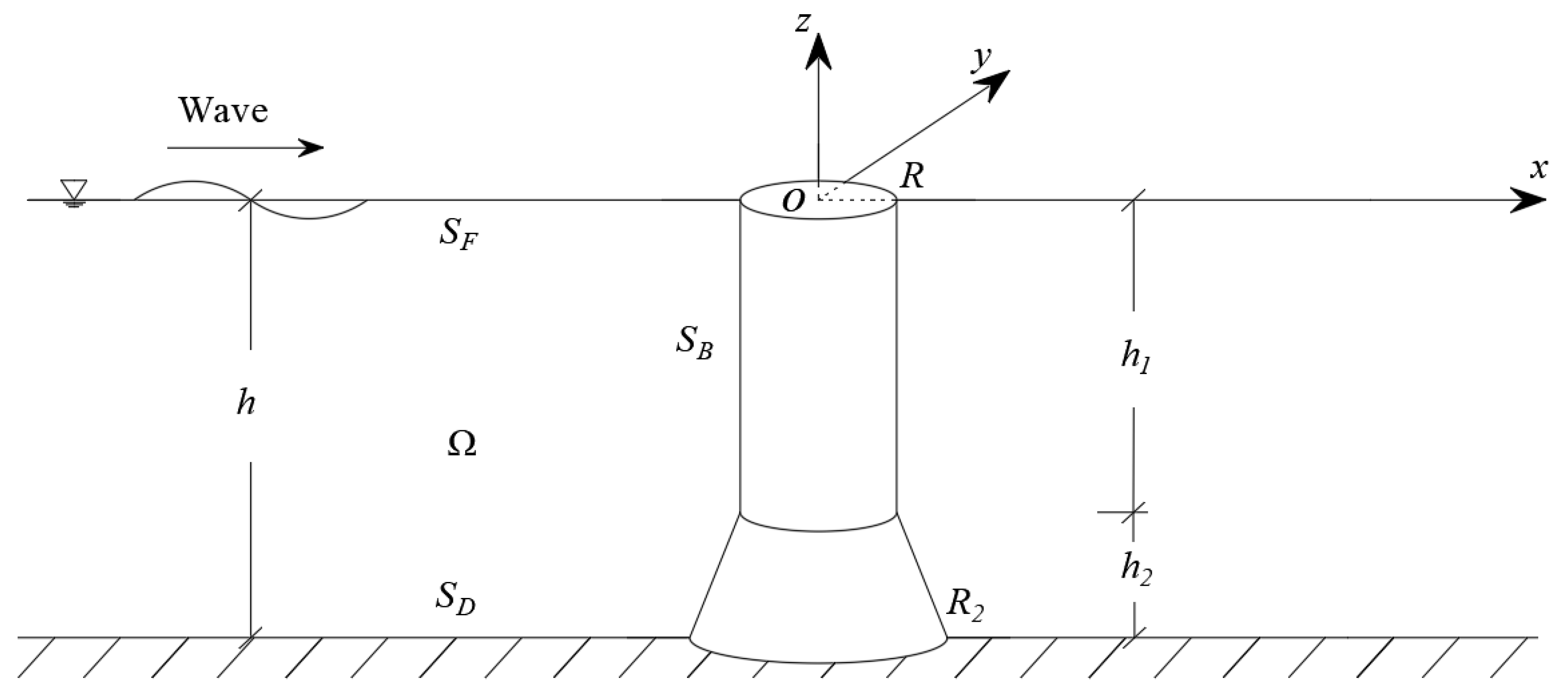
To address the challenges of withstanding strong nonlinear wave loads in deeper water environments while maintaining cost-effectiveness, Ma and Yang [3] introduced an innovative composite monopile foundation incorporating CFDST structures. As illustrated in Figure 1, this design reduces wave loads through strategic diameter reduction at the water surface. The CFDST system, comprising concentrically arranged steel tubes with interposed concrete infill [4,5,6], has demonstrated its effectiveness as a high-strength component in bridge piers and offshore platform support columns [7,8,9]. The adoption of dual steel tubes endows this CFDST system with superior strength and enhanced ductility compared to conventional reinforced concrete systems, while demonstrating reduced steel consumption and lower construction costs relative to jacket structures. Ma and Yang [3] carried out systematic investigations into the vibrational behavior and the ultimate load-bearing capacity of the hybrid monopile using CFDST. However, they utilized a simplified Morison’s equation to evaluate the wave forces on the hybrid monopile, which is considered to be limited.

Morison’s equation, initially developed by Morison et al. [10], was primarily designed for estimating linear wave forces on small-diameter piles. The method operates under the assumption that the pile’s presence negligibly affects wave motion, calculating water particle velocity and acceleration based solely on the incident wave field. The resultant structural loading principally comprises inertia forces and drag forces. However, this methodology presents significant limitations when applied to large-scale structures or strongly nonlinear wave conditions [11,12,13]. Specifically, Morison’s equation tends to underestimate peak forces on fixed cylinders in such scenarios. Given that the CFDST hybrid monopile is specifically designed for deployment in areas characterized by strong nonlinear waves and features a substantial pile diameter, Morison’s equation proves inadequate for accurately simulating its hydrodynamic performance.

Numerous advanced modeling techniques and computational methods have been formulated to analyze the complex coupling mechanisms of strongly nonlinear waves with large-scale monopile foundations, such as the computational fluid dynamics (CFD) method and fully nonlinear potential flow theory, etc. The CFD methodologies offer the capability to simulate strongly nonlinear free surface flows, providing detailed insights into various flow characteristics. Paulsen et al. [14] implemented a numerical wave flume using the open-source CFD platform OpenFOAM, conducting systematic investigations into higher-order harmonic hydrodynamic loading on vertical cylindrical structures in strongly nonlinear wave conditions. However, CFD methods require substantial computational resources and time to achieve high-fidelity solutions.

The fully nonlinear potential flow theory provides an alternative approach where both water surface and structural surface boundary conditions are satisfied instantaneously, theoretically accounting for all nonlinear factors in wave–structure interactions. Its computational efficiency is dozens of times that of CFD and has acceptable accuracy. The foundations of this approach can be traced to the pioneering work of Longuet-Higgins and Cokelet [15]. Subsequent developments include Yang and Ertekin’s [16] implementation of the constant BEM to establish a 3D fully nonlinear numerical wave flume, enabling simulation of nonlinear diffraction around vertical cylinders subjected to solitary and Stokes waves. Significant advancements were made by Ferrant [17] and Ferrant et al. [18], who developed a numerical model for fully nonlinear interactions between open water waves and structures using an incident-scattered wave separation approach. Bai and Eatock Taylor made substantial contributions through their series of studies [19,20,21], employing HOBEM to construct comprehensive three-dimensional fully nonlinear numerical wave tanks. Their work encompassed investigations into wave radiation from oscillating vertical cylinders and detailed modeling of fully nonlinear coupling between waves and both fixed and floating structures. Liang et al. [22,23] applied fully nonlinear theory to the hydroelastic problem and developed a time-dependent wave–plate interaction model.

This study establishes a time-dependent potential flow model to examine the coupling of fully nonlinear waves with fixed offshore structures. Following rigorous validation, the model is utilized to examine the hydrodynamic characteristics of a CFDST hybrid monopile under extreme nonlinear wave conditions. The research focuses on qualitative analysis of wave load and wave run-up phenomena on the hybrid monopile under nonlinear wave action, and on critical evaluation of the limitations inherent in Morison’s equation for such applications. Furthermore, this study presents a systematic evaluation of the advantageous effects of CFDST structural implementation on offshore monopile wind turbine design, particularly in terms of wave run-up and wave load mitigation.

2. Mathematical Formulation

The current investigation addresses nonlinear wave interactions with the above composite monopile, which uses CFDST in a 3D fluid domain $\Omega$, and focuses on the nonlinear wave loads on the structure. The computational domain employs a Cartesian coordinate system Oxyz, as illustrated in Figure 2, with its origin positioned at the undisturbed free surface and the positive z-axis vertically oriented. The computation domain $\Omega$ is bounded by a water surface $S_F$, a flat seabed surface $S_D$ and the side surface of the monopile $S_B$.

2.1. Boundary Value Problem

It is assumed the fluid is inviscid and incompressible with irrotational flow, establishing the existence of a velocity potential $\mathsf{\varphi }(x,y,z,t)$ within the fluid domain $\Omega$ that satisfies Laplace’s equation:

$${\nabla }^2\mathsf{\varphi }=0,\mathrm{in} \Omega .$$

(1)

At the air–water interface $S_F$, the velocity potential is governed by the fully nonlinear dynamic and kinematic conditions

$$\left\{\begin{array}{c}\partial \mathsf{\eta }/\partial t=\partial \mathsf{\varphi }/\partial z-\nabla \mathsf{\varphi }·\nabla \mathsf{\eta },\\ \partial \mathsf{\varphi }/\partial t=-g\mathsf{\eta }-{\displaystyle \frac{1}{2}}\left(\nabla \mathsf{\varphi }·\nabla \mathsf{\varphi }\right),\end{array}\right.\mathrm{on} S_F,$$

(2)

where g is the gravitational acceleration and $\mathsf{\eta }(x,y,t)$ is the wave elevation.

At the impermeable seabed boundary, $\mathsf{\varphi }(x,y,z,t)$ satisfies:

$${\left.{\displaystyle \frac{\partial \mathsf{\varphi }}{\partial z}}\right|}_{z=-h}=0, \mathrm{on} S_D.$$

(3)

At the structural interface $S_B$, the velocity continuity condition in the normal direction necessitates:

$${\displaystyle \frac{\partial \mathsf{\varphi }}{\partial n}}=0, \mathrm{on} S_B.$$

(4)

The structure is fixed so the velocity is zero.

To efficiently resolve the three-dimensional hydrodynamic problem, the wave scattering decomposition method [13,18] is implemented. Therefore, the total velocity potential $\mathsf{\varphi }(x,y,z,t)$ and water surface elevation $\mathsf{\eta }(x,y,t)$ are separated using the following decomposition technique

$$\left\{\begin{array}{c}\mathsf{\varphi }={\mathsf{\varphi }}_I+{\mathsf{\varphi }}_S\\ \mathsf{\eta }={\mathsf{\eta }}_I+{\mathsf{\eta }}_S\end{array}\right.$$

(5)

where the incident components $\left({\mathsf{\varphi }}_I,{\mathsf{\eta }}_I\right)$ are defined as known solutions through technique of flow decomposition [17], leaving only the scattered components $\left({\mathsf{\varphi }}_S,{\mathsf{\eta }}_S\right)$ requiring determination.

For the diffraction problem of fixed structures, the semi-Lagrangian approach with higher computational efficiency can be utilized. This solely necessitates monitoring the vertical displacements of grid points on $S_F$. A specialized temporal differentiation operator is formulated as:

$${\displaystyle \frac{\mathsf{\delta }}{\mathsf{\delta }t}}={\displaystyle \frac{\partial }{\partial t}}+\left(0,0,{\displaystyle \frac{\mathsf{\delta }\mathsf{\eta }}{\mathsf{\delta }t}}\right)·\nabla .$$

(6)

Application of the decomposition methodology and the specifically defined temporal derivative operator to Equation (2) yields the boundary conditions for the scattered wave component on the water surface

$${\displaystyle \frac{\mathsf{\delta }{\mathsf{\eta }}_S}{\mathsf{\delta }t}}=-{\displaystyle \frac{\partial {\mathsf{\eta }}_I}{\partial t}}+{\displaystyle \frac{\partial {\mathsf{\varphi }}_I}{\partial z}}+{\displaystyle \frac{\partial {\mathsf{\varphi }}_S}{\partial z}}-\nabla \left({\mathsf{\varphi }}_I+{\mathsf{\varphi }}_S\right)·\nabla \left({\mathsf{\eta }}_I+{\mathsf{\eta }}_S\right)-V(r){\mathsf{\eta }}_S$$

(7)

$${\displaystyle \frac{\mathsf{\delta }{\mathsf{\varphi }}_S}{\mathsf{\delta }t}}=-{\displaystyle \frac{\partial {\mathsf{\varphi }}_I}{\partial t}}-g({\mathsf{\eta }}_I+{\mathsf{\eta }}_S)-{\displaystyle \frac{1}{2}}\left[\nabla \left({\mathsf{\varphi }}_I+{\mathsf{\varphi }}_S\right)·\nabla \left({\mathsf{\varphi }}_I+{\mathsf{\varphi }}_S\right)\right]+{\displaystyle \frac{\mathsf{\delta }({\mathsf{\eta }}_I+{\mathsf{\eta }}_S)}{\mathsf{\delta }t}}{\displaystyle \frac{\partial {\mathsf{\varphi }}_S}{\partial z}}-V(r){\mathsf{\varphi }}_S$$

(8)

where $V(r)$ is the damping coefficient. Figure 3 shows the artificial damping zone:

$$V(r)=\left\{\begin{array}{ll}{\mathsf{\alpha }}_0\mathsf{\omega }{\left({\displaystyle \frac{r-r_0}{{\mathsf{\beta }}_0\mathsf{\lambda }}}\right)}^2,& r_0\le r\le r_D=r_0+{\mathsf{\beta }}_0\mathsf{\lambda }\\ 0,r<r_0\end{array}\right..$$

(9)

The artificial damping zone is configured as an annular region at the outermost periphery of the circular computational domain, while the offshore structure is positioned at the computational domain’s geometric center.

Within the damping layer, ${\mathsf{\varphi }}_S$ gradually lose their energy as they propagate. $\mathsf{\lambda }$ is a representative wavelength. Parameter ${\mathsf{\alpha }}_0$ regulates the attenuation intensity within the damping region. A higher value of ${\mathsf{\alpha }}_0$ would cause waves to dissipate more rapidly within the damping zone. Parameter ${\mathsf{\beta }}_0$ determines the width of the damping zone. A larger value of ${\mathsf{\beta }}_0$ could potentially provide more space for waves to dissipate before reaching the boundaries of the simulation domain. In the present study, ${\mathsf{\alpha }}_0$ and ${\mathsf{\beta }}_0$ have been set to 1.0.

In addition, ${\mathsf{\varphi }}_S$ fulfills the Neumann boundary requirement on a rigid surface:

$${\displaystyle \frac{\partial {\mathsf{\varphi }}_S}{\partial n}}=-{\displaystyle \frac{\partial {\mathsf{\varphi }}_I}{\partial n}},\begin{array}{cc}& \end{array} \mathrm{on} S_D,S_B,$$

(10)

Considering the temporal-domain solution framework, the initial parameters should be set as:

$${\mathsf{\varphi }}_S=0,{\mathsf{\eta }}_S=0, \mathrm{at} t=0.$$

(11)

2.2. Boundary Integral Equation Method

The nonlinear boundary value problem is resolved through implementation of the boundary integral equation (BIE) method. By applying Green’s second identity to ${\mathsf{\varphi }}_S$ over the closed boundary $S_{\Omega }$, the governing integral equation is formulated as

$$\mathsf{\alpha }(x_0){\mathsf{\varphi }}_S(x_0)={\displaystyle \underset{S_{\Omega }}{\iint }\left[{\mathsf{\varphi }}_S(x)\frac{\partial G(x;x_0)}{\partial n}-G(x;x_0)\frac{\partial {\mathsf{\varphi }}_S(x)}{\partial n}\right]\mathrm{d}s}$$

(12)

where $x$ are source points $(x_0,y_0,z_0)$, $x_0$ are field points $(x,y,z)$ and $\mathsf{\alpha }$ is the solid angle coefficient. A Rankine source combined with its mirrored counterparts relative to the seabed ($z=-h$) could be utilized as the Green’s function $G(x,x_0)$. Then the integral Equation (12) can be discretized using HOBEM. The specific solving process is referred to in the author’s previous article [23].

2.3. Hydrodynamic Forces

Following the computation of velocity potential and its spatial gradients at each temporal iteration, hydrodynamic pressure distribution on the structural surface is determined through application of the Bernoulli equation:

$$p=-\mathsf{\rho }\left({\mathsf{\varphi }}_t+{\displaystyle \frac{1}{2}}{\left|\nabla \mathsf{\varphi }\right|}^2+gz\right)$$

(13)

Therefore, the wave forces (f₁, f₂, f₃) and moments (f₄, f₅, f₆) are determined by integrating the pressure on structure surface, taking into account both their magnitudes and directions

$$f_i={\displaystyle \underset{S_B}{\iint }p{n}_i\mathrm{ds}}=-\mathsf{\rho }{\displaystyle \underset{S_B}{\iint }\left({\mathsf{\varphi }}_t+\frac{1}{2}{\left|\nabla \mathsf{\varphi }\right|}^2+gz\right)n_i\mathrm{ds}}\left(i=1,\dots ,6\right)$$

(14)

where $\mathsf{\rho }$ represents the fluid mass density and $n_i$ are the normalized directional vector components.

It should be emphasized that, while the spatial velocity gradients $\nabla \mathsf{\varphi }$ on the structural surface can be numerically obtainable [23], accurate determination of the ${\mathsf{\varphi }}_t$ remains computationally challenging. Accurate temporal derivative computation is essential for reliable hydrodynamic pressure and force determination. This study employs dual numerical approaches: a novel backward differentiation scheme incorporating mesh displacement effects and the established indirect method [23]. Cross-validated results from these independent methodologies ensure robust computation of transient hydrodynamic parameters.

In the novel backward differentiation scheme, by applying the particular operator $\mathsf{\delta }/\mathsf{\delta }t=\partial /\partial t+v_{\mathrm{mesh}}·\nabla$ as in Equation (6), the ${\mathsf{\varphi }}_t$ can be expressed as

$${\mathsf{\varphi }}_t={\displaystyle \frac{\partial {\mathsf{\varphi }}_I}{\partial t}}+{\displaystyle \frac{\partial {\mathsf{\varphi }}_S}{\partial t}}={\displaystyle \frac{\partial {\mathsf{\varphi }}_I}{\partial t}}+{\displaystyle \frac{\mathsf{\delta }\mathsf{\varphi }}{\mathsf{\delta }t}}-v_{\mathrm{mesh}}·\nabla {\mathsf{\varphi }}_S$$

(15)

where $v_{\mathrm{mesh}}$ denotes the grid velocity on the structure surface and $\mathsf{\delta }{\mathsf{\varphi }}_S/\mathsf{\delta }t$ is computed by a backward differentiation method using velocity potentials from current and prior temporal steps.

2.4. Numerical Modeling

2.4.1. Initial Grid Generation

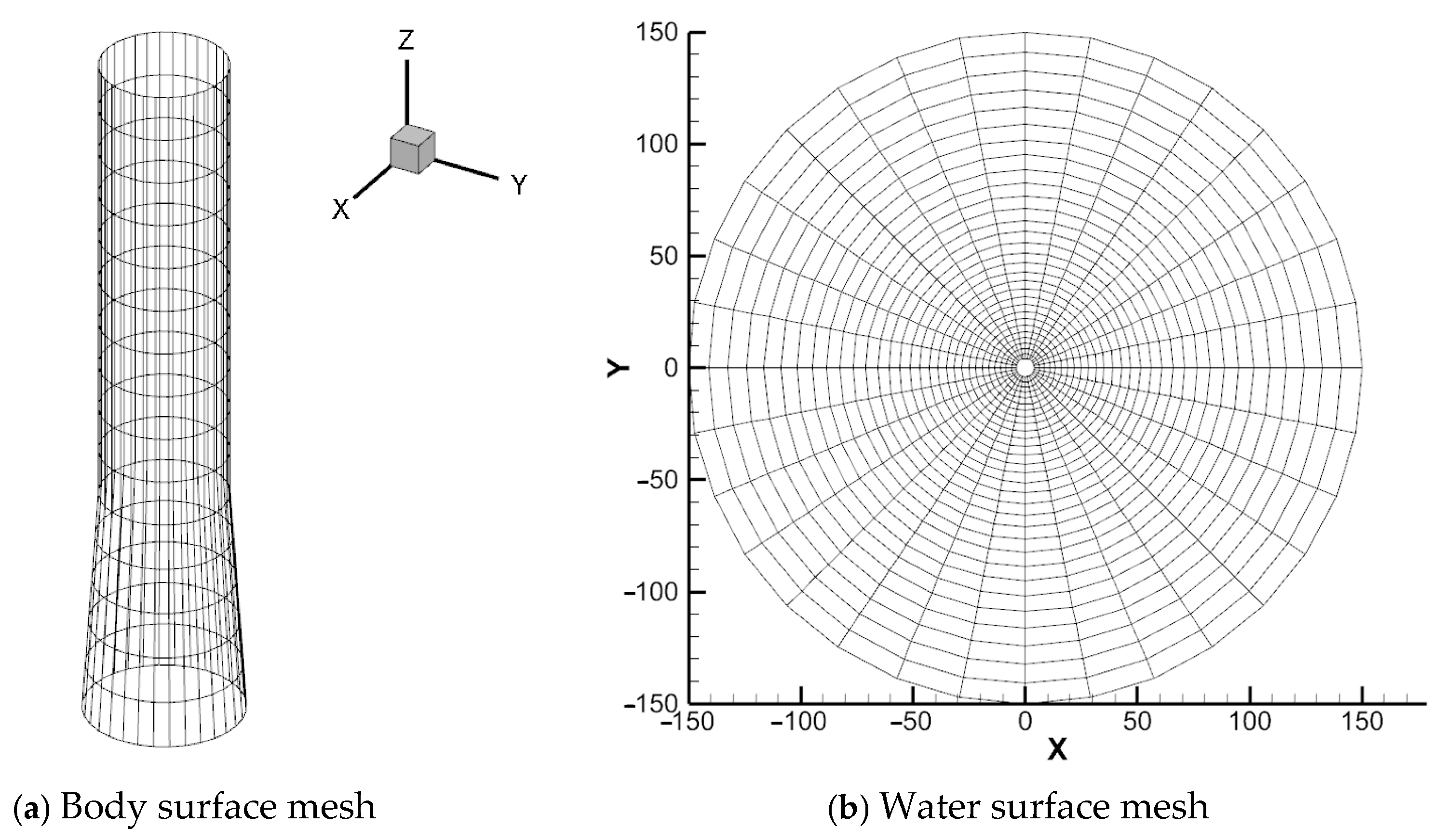
The numerical model employs quadratic isoparametric boundary elements for spatial discretization of both water surface and body surface. Adaptive grid refinement is implemented on the free-surface domain, featuring higher grid density proximal to the structure with gradual coarsening in far-field regions. Figure 4 provides a diagram of the initial computational mesh configuration.

The computational domain radius is typically set to three wavelengths to accommodate a one-wavelength-wide damping zone. Body-fitted meshes and adjacent free-surface elements are generally refined below one-tenth of the incident wavelength, with surface grid size progressively coarsening as distance from the structure increases.

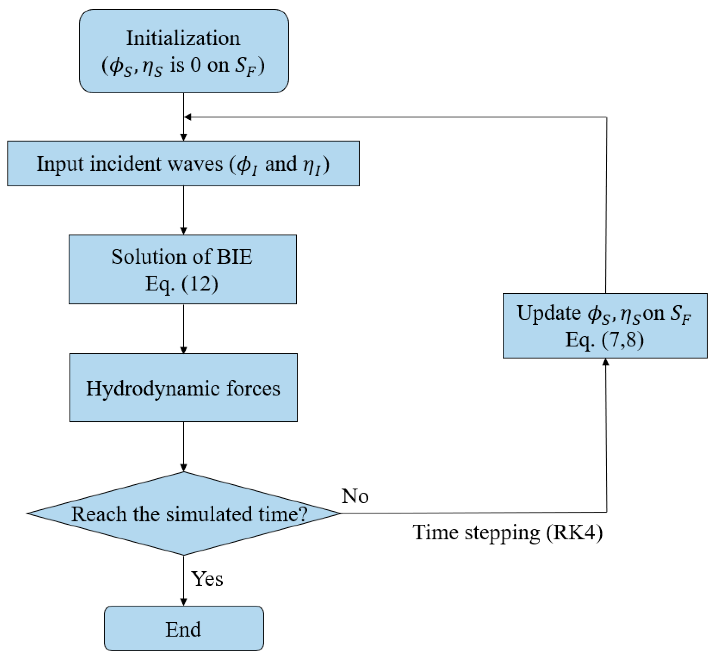
2.4.2. Time-Stepping Scheme

Following resolution of the boundary value problem, fluid velocity components at the current temporal iteration are obtained across the free surface. Temporal integration of the fully nonlinear free-surface condition is subsequently performed to advance both wave elevation and velocity potential to the next time step. The numerical implementation employs a fourth-order Runge–Kutta (RK4) time discretization scheme, demonstrating superior accuracy and numerical stability characteristics for strongly nonlinear hydrodynamic simulations. The RK4 scheme permits larger time steps while maintaining high numerical accuracy, achieving an optimal balance between computational efficiency and solution precision. Its enhanced stability and broad applicability make it particularly suitable for complex dynamic systems.

To achieve progressive initialization and mitigate sudden condition transitions during simulation commencement, a ramp function $R_m$ [24] is applied

$$R_m=\left\{\begin{array}{ll}{\displaystyle \frac{1}{2}}\left[1-\cos \left({\displaystyle \frac{\mathsf{\pi }t}{T_m}}\right)\right]& ,t\le T_m\\ 1& ,t>T_m\end{array}\right..$$

(16)

where $T_m$ is generally an integer multiple of the wave period, and $T_m$ is two times the wave period in the present model.

2.4.3. Mesh Deformation

At each temporal iteration, both water surface and body surface grids undergo coordinate updating. Implementation of the semi-Lagrangian tracking methodology for water surface node motion restricts grid adjustments to vertical coordinate reinitialization per time step. This constrained kinematic updating protocol streamlines the computational workflow by eliminating horizontal node displacement calculations, significantly enhancing numerical efficiency while maintaining geometric consistency.

The wetted surface geometry evolves dynamically with waterline nodal displacements. To preserve grid quality during geometric deformation, a spring analogy mesh deformation technique is implemented. Spring equilibrium lengths correspond to initial edge dimensions, ensuring nodal force equilibrium in the initial configuration. Node displacements are governed by Hooke’s law, with the resultant force at node i expressed as

$$F_i={\displaystyle \sum _{j=1}^{N_i}{K}_{ij}\left({\delta }_j-{\delta }_i\right)}$$

(17)

where K_ij denotes the spring stiffness coefficient between nodes i and j, δ_i and δ_j represent the nodal displacement vectors and N_i indicates the number of neighboring nodes connected to node i. Enforcing static equilibrium conditions requires the resultant force vector at each displaced node to vanish, yielding the Jacobi iterative formulation for nodal displacement determination:

$${\delta }_i^{k+1}={\displaystyle \frac{{\displaystyle \sum _{j=1}^{N_i}{K}_{ij}{\delta }_j^k}}{{\displaystyle \sum _{j=1}^{N_i}{K}_{ij}}}}$$

(18)

The elastic coefficient can be written as

$$K_{ij}={\displaystyle \frac{1}{l_{ij}^2}}$$

(19)

where

$$l_{ij}=\sqrt{{\left(x_i-x_j\right)}^2+{\left(y_i-y_j\right)}^2+{\left(z_i-z_j\right)}^2}$$

(20)

After multiple iterations of Equation (18) and a convergence of results, the final coordinates of node i are:

$$x_i^{\mathrm{new}}=x_i^{\mathrm{old}}+{\delta }_i^{k,\mathrm{final}}$$

(21)

2.4.4. Numerical Implementation Process

To outline the solution algorithm, a process diagram is incorporated to delineate the computational steps, as shown in Figure 5.

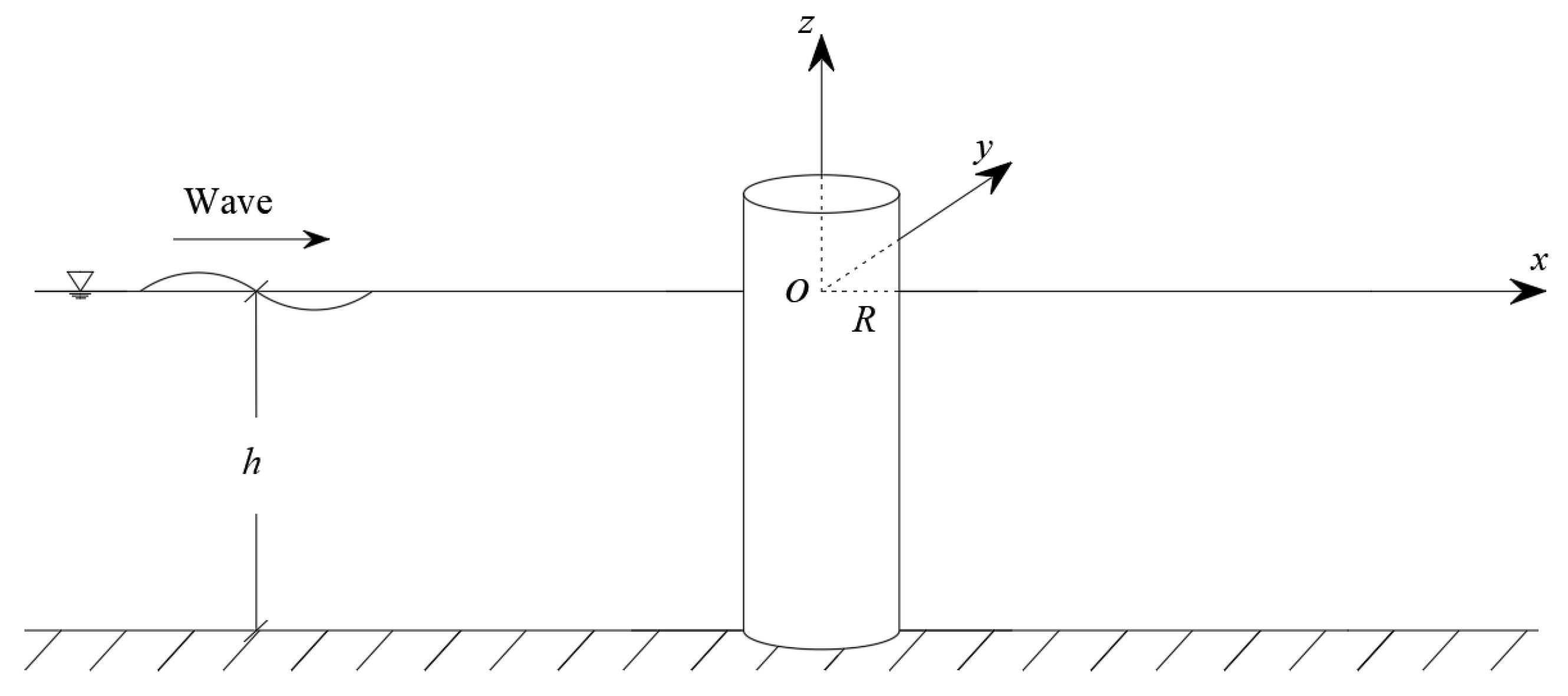
3. Model Validation

In this section, the numerical model is a vertical cylinder subjected to a fully nonlinear wave, as shown in Figure 6. In Section 3 of the author’s previous article [23], the great accuracy of our model in simulating the wave run-up around a vertical cylinder subjected to a fully nonlinear wave was shown. To further verify the correctness of our model in calculating wave force on a structure, we compare present wave force results with the experimental data of Huseby and Grue [25] and the numerical solutions of Ferrant [17]. Here, the water depth h is 0.6 m, the radius of the vertical cylinder $R=0.03 \mathrm{m}$, the draft is 0.6 m and the dimensionless parameter kR is 0.245.

Fourier transformation of horizontal force time series yields each order’s hydrodynamic load components. Figure 7 illustrates the variation of the dimensionless first- and second-order wave forces in relation to the wave steepness, kA. The maximum kA considered in the present analysis is 0.135, as significant variations in the water nodes at the waterline occur at higher steepness values, leading to potential numerical instability.

As illustrated in Figure 7, the present results demonstrate overall agreement with Ferrant’s numerical simulations [17] and Huseby’s experimental data [25]. Discrepancies between the numerical results arise from methodological differences: Ferrant’s fully nonlinear model employs conventional boundary element meshing, whereas the current approach utilizes a higher-order boundary element method combined with a spring approximation technique on structural surfaces. Both the present model and Ferrant’s first-order results show excellent consistency with Huseby’s experimental measurements, where the second-order components exhibit constant offsets. At small kA, the time-domain numerical results from both the current and Ferrant’s models align closely with Newman’s [26] frequency-domain second-order reference value of 0.59. Perhaps due to the small step of the wave, it is difficult to accurately extract a small part of the experimental time series.

4. Results and Discussion

Upon successful model verification, the numerical model established was employed to analyze the complex coupling of fully nonlinear waves with the novel CFDST hybrid monopile foundation. Here, the water depth h = $45 \mathrm{m}$, the water density $\mathsf{\rho }=1023{ \mathrm{kg}/\mathrm{m}}^3$, the radius of CFDST R = 4 m, the height of CFDST h₁ = 30 m, the radius of monopile bottom R₂ = 5 m and the height of the transition segment h₂ = 15 m.

4.1. Convergence Study

We selected a representative case with k = 0.12 and kA = 0.12. The convergence analysis was conducted in two phases: spatial discretization and temporal discretization.

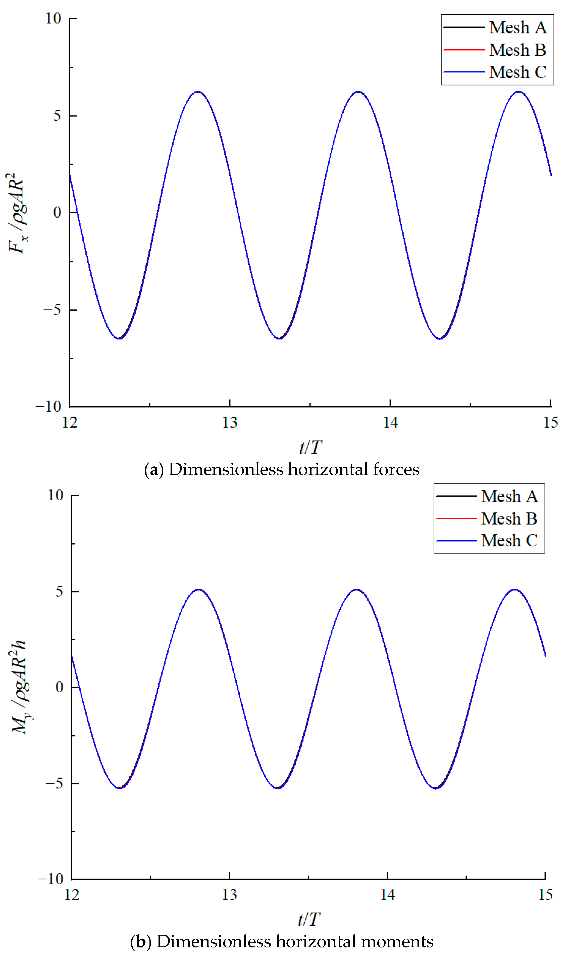
Initially, we performed a spatial convergence analysis using three progressively refined mesh configurations, designated as Mesh A, Mesh B and Mesh C. The characteristic parameters of these meshes are detailed in

Table 1. Quantity of elements and nodes in varied grid systems.

	Elements on Structure Surface	Elements on Water Surface	Nodes on Whole Surface
Mesh A	240	480	2360
Mesh B	360	720	3488
Mesh C	480	960	4616

. To ensure numerical accuracy, the computational domain was designed to maintain a free propagation distance for scattered waves of at least three wavelengths in all directions.

Figure 8 illustrates the computed wave forces for each mesh configuration, where the horizontal moment My is referenced to the center point of the pile bottom. The results demonstrate rapid numerical convergence, with Mesh A producing results that are virtually identical to those obtained from the finer meshes (Mesh B and Mesh C). This convergence behavior indicates that Mesh A provides an optimal balance between computational accuracy and efficiency.

Subsequently, we conducted a temporal convergence analysis using a time step of Δt = T/60, T/90 and T/120, where T represents the wave period. The temporal convergence patterns mirrored those observed in the spatial analysis. Based on these comprehensive convergence tests, the combination of Mesh A with a time step of Δt = T/60 was determined as providing sufficient numerical accuracy for subsequent simulations.

4.2. The Significance of the Wave Nonlinearity

The initial phase of our investigation focuses on examining the significance of wave nonlinearity on both the hydrodynamic forces and the wave run-up acting on the hybrid monopile. This analysis was conducted using incident waves with varying wave steepness parameters. This study employs three dimensionless wave numbers (kR) combined with three distinct wave steepness values (kA = 0.04, 0.08 and 0.12). For comparative purposes, we included horizontal wave force and moments calculations derived from Morison’s equation.

The accurate calculation of wave force has a significant influence on engineering design. Underestimation of wave load will lead to unsafe engineering design, while overestimation of wave load will incur additional costs.

Figure 9 presents the temporal variation of dimensionless wave forces and moments on the CFDST hybrid monopile for kR values of 0.20, 0.48 and 0.60. At low wave steepness conditions, the wave forces and moments profile maintains a sinusoidal pattern. However, as wave steepness increases, the wave forces and moments curves exhibit pronounced nonlinear characteristics, manifested by a significant amplification of the trough amplitude. This discrepancy becomes particularly pronounced in cases with smaller kR values.

Furthermore, Morison’s equation exhibits inherent limitations in its computational methodology. The first point is the applicability range. As demonstrated in Figure 8, the equation is only valid for small kR values. When kR increases (e.g., kR = 0.6), wave diffraction effects become significant, rendering Morison’s equation inadequate for accurate wave force calculations on cylindrical structures. The second point is wave steepness dependency. For kR = 0.2, the equation’s predictions align with nonlinear model results only under small wave steepness conditions. Its accuracy deteriorates significantly with increasing wave steepness, failing to provide reliable wave force estimates. The last point is reference point limitation. Morrison’s equation takes the center of the structure as the reference point, while the method in the present study conducts the calculation on the actual wet surface of the structure, which leads to substantial phase discrepancies in the calculation results. This phase difference becomes increasingly pronounced at larger kR values, further compromising the method’s reliability. These limitations collectively underscore the need for the present approach, particularly when analyzing wave–structure interactions under conditions of large kR values or significant wave steepness.

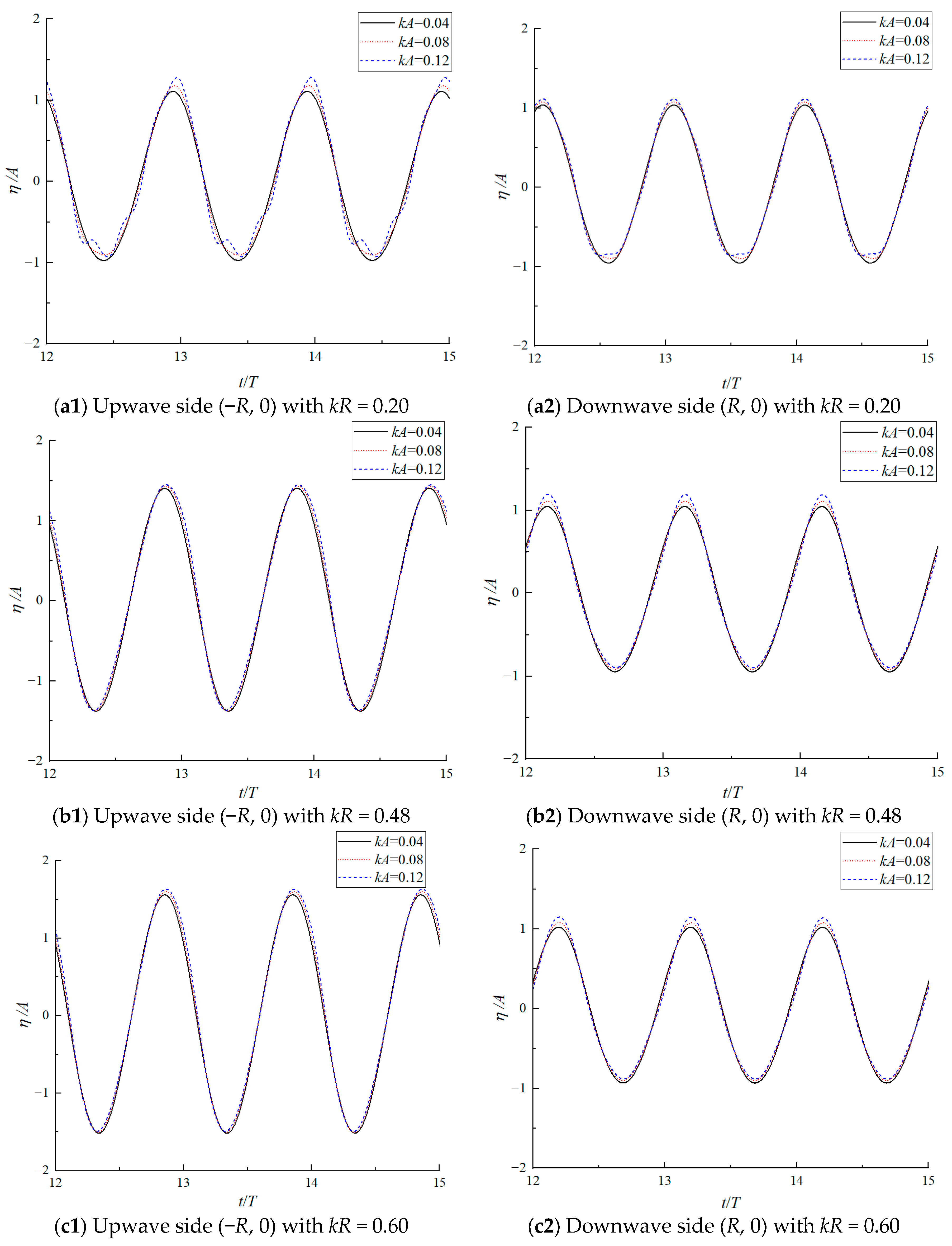
In the design of monopile foundations for offshore wind turbines, the study of wave run-up is of crucial significance. If the wave run-up approaches the flange of the transition section, it may cause the vibration of the tower to be transmitted to the nacelle, affecting the power generation efficiency. Under extreme conditions, wave run-up may even approach the top of the tower, causing seawater to invade electrical equipment.

Figure 10 presents the temporal variation of wave run-up on the CFDST hybrid monopile for kR = 0.20, 0.48 and 0.60. At lower wave steepness, the temporal variation of the wave run-up closely approximates a sinusoidal curve. However, as wave steepness increases, the crest of the wave run-up curve becomes more pronounced while the trough exhibits a smoother profile. This nonlinear behavior in wave run-up is particularly evident at smaller kR values.

However, Morison’s equation proves inadequate for predicting wave run-up phenomena and, consequently, no comparative results from this method are available. Nevertheless, wave run-up remains a critical parameter in offshore wind turbine design, requiring careful consideration in structural analysis and safety assessments.

4.3. The Influence of the Outer Diameter Ratio

The outer diameter ratio R/R₂, denoted as p, represents a critical design parameter that substantially influences the hybrid monopile’s performance. Three distinct values of p were examined to evaluate their impacts: 1.0, 0.8 and 0.6. The analysis maintained a constant monopile bottom radius R₂ of 5 m, with a wave number k of 0.12 and wave steepness kA of 0.12. Among them, the hydrodynamic characteristics in the case of the outer diameter ratio “p = R/R₂ = 1.0” are the same as those of the traditional vertical large-diameter monopile foundation.

The total pressure consists of hydrostatic pressure and dynamic pressure. Due to the symmetry of the structure, the wave forces generated by the circumferential hydrostatic pressure cancel each other out and have no effect on the total wave force. Figure 11 depicts the dynamic pressure magnitude profiles across the surface of the hybrid monopile for different outer diameter ratios p. While the pressure distribution patterns show considerable similarity across various p values, the pressure magnitude demonstrates a progressive decrease with depth towards the seabed. Notably, peak dynamic pressures occur near the water surface on both the upwave and downwave sides. The maximum recorded pressures are 14,046 Pa, 15,162 Pa and 16,985 Pa for p values of 0.6, 0.8 and 1.0, respectively. This pressure reduction correlates with the decreased pile diameter. Additionally, the decreased pile diameter means that the area of the structure exposed to pressure is smaller. All these will lead to a decrease in the total wave force on the structure.

As demonstrated in Figure 12, reducing the outer diameter ratio p causes a substantial reduction in both the total wave forces and the corresponding moments acting on the hybrid monopile. The implementation of CFDST material in the hybrid monopile design, combined with the reduction of the outer diameter ratio p, effectively achieves significant wave load mitigation. In monopile offshore wind turbine design, a reduction in wave load on a structure implies that the structure becomes relatively stronger with enhanced safety, while also enabling a further decrease in the use of high-strength materials like steel to reduce costs.

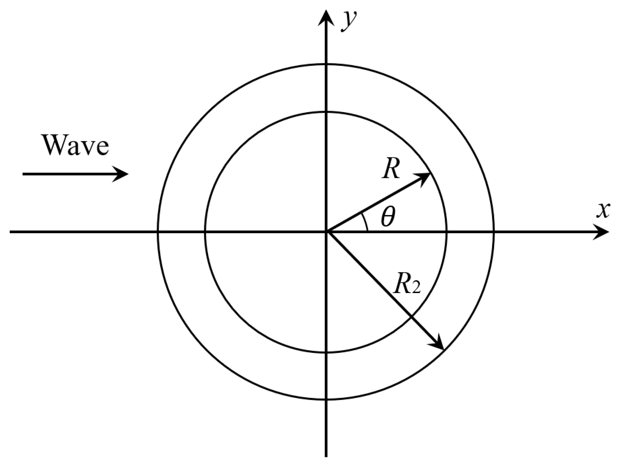
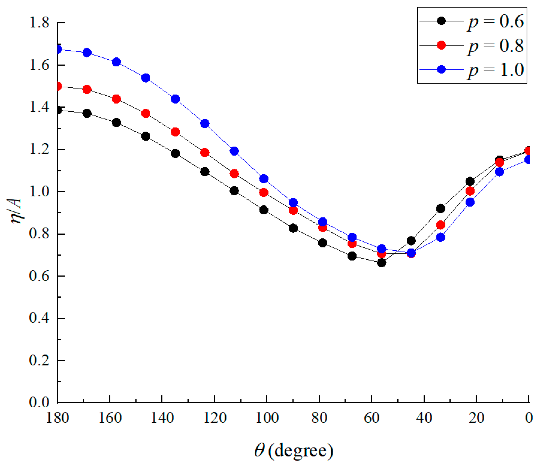
Figure 13 illustrates the definition of the azimuth angle $\mathsf{\theta }$ around the circular cylinder, measured in an anticlockwise direction. Here, $\mathsf{\theta }$ = 180° corresponds to the upwave side, while $\mathsf{\theta }$ = 0° represents the downwave side. Figure 14 presents the wave run-up profiles around the hybrid monopile for various outer diameter ratios p. It is evident that a smaller outer diameter ratio p results in a reduced wave run-up around the hybrid monopile, with this effect being particularly pronounced on the upwave side.

Figure 15 further depicts the temporal variation of dimensionless wave run-up on both the upwave and downwave sides of the hybrid monopile for different outer diameter ratios p. Although a smaller p corresponds to a smaller kR, as discussed in Section 4.2, the temporal variation of wave run-up on the upwave side exhibits higher nonlinearity. Nevertheless, the peak values remain lower compared to cases with larger p values.

The utilization of CFDST material in the hybrid monopile significantly reduces wave run-up by decreasing the outer diameter ratio p. In monopile offshore wind turbine design, a reduction in wave run-up leads to lower probabilities of wave impact on the flange causing tower–nacelle vibrations or wave intrusion into the nacelle, thereby improving safety. This also allows for further lowering of the required height of the flange and tower sections, reducing material usage and thus lowering costs.

5. Conclusions

This study investigates the nonlinear wave–structure coupling between fully nonlinear waves and a CFDST composite monopile through a potential flow model. The computational framework incorporates a RK4 scheme combined with semi-Lagrangian free surface updating, while HOBEM is implemented to address boundary value problems per temporal iteration. Following comprehensive validation, the numerical model is employed to analyze the hydrodynamic characteristics of the CFDST hybrid monopile under extreme nonlinear wave conditions. The conclusions are outlined below:

• The numerical model exhibits strong consistency with both of the other numerical solutions and experimental results in predicting fully nonlinear wave run-up and wave force characteristics. This strong correlation across multiple validation cases confirms the accuracy and reliability of the proposed computational model.
• For the CFDST hybrid monopile deployed in large-scale installations within deep-water environments characterized by strong nonlinear waves, the application of the present nonlinear model is essential for accurate computational analysis. Morison’s equation, being fundamentally based on linear theory and neglecting wave diffraction effects, demonstrates limited applicability. It provides reliable predictions only when both the kR value and wave steepness remain sufficiently small. These inherent limitations render Morison’s equation inadequate for analyzing the complex wave–structure interactions encountered by CFDST hybrid monopiles in challenging offshore environments.
• As wave steepness increases, the trough amplitude of the wave force curve is significantly amplified, and the crest of the wave run-up curve becomes more pronounced while the trough exhibits a smoother profile. This nonlinear behavior is particularly evident at the smaller kR values of the CFDST hybrid monopile.
• The implementation of CFDST material in the hybrid monopile design, combined with the reduction of the outer diameter ratio p, effectively achieves significant wave load mitigation and significantly reduces wave run-up, contributing to safer and more cost-effective design solutions for offshore wind turbine foundations.
• Last but not least, for the CFDST hybrid monopile, further studies can still be carried out, such as considering the elastic deformation of the monopile in the hydrodynamic analysis and conducting hydrodynamic model experiments.