Predicting Energy Consumption and Time of Use of Home Appliances in an HEMS Using LSTM Networks and Smart Meters: A Case Study in Sincelejo, Colombia

Abstract

Rising household electricity consumption, driven by technological advances and increased indoor activity, has led to higher energy costs and an increased reliance on non-renewable sources, exacerbating the carbon footprint. Home energy management systems (HEMS) are positioning themselves as an efficient alternative by integrating artificial intelligence to improve their accuracy. Predictive algorithms that provide accurate data on the future behavior of energy consumption and appliance usage time are required in these HEMS to achieve this goal. This study presents a predictive model based on recurrent neural networks with long short-term memory (LSTM), known to capture nonlinear relationships and long-term dependencies in time series data. The model predicts individual and total household energy consumption and appliance usage time. Training data were collected for 12 months from an HEMS installed in a typical Colombian house, using smart meters developed in this research. The model’s performance is evaluated using the mean squared error (MSE), reaching a value of 0.0168 kWh². The results confirm the effectiveness of HEMS and demonstrate that the integration of LSTM-based predictive models can significantly improve energy efficiency and optimize household energy consumption.

1. Introduction

Household electricity consumption has been growing steadily, driven primarily by technological advances, increasing the adoption of electronic devices and increasing indoor time. According to the International Energy Agency (IEA), appliances and cooling systems, along with connected devices, account for a significant portion of the increase in residential consumption. In addition, factors such as urban population growth and access to more sophisticated technologies have expanded energy demand [1]. This growing demand for electricity in homes directly impacts global energy consumption, increasing greenhouse gas emissions and hindering efforts to achieve sustainability goals. Addressing this problem requires the adoption of efficient energy management strategies and digital tools that enables more sustainable electricity consumption. In Colombia, the recent trends in energy demand reflect an increase due to the greater use of electrical devices in the home. This is related to a change in habits, such as spending more time indoors, which has led to a sustained increase in residential energy consumption [2]. Studies by the Mining and Energy Planning Unit (UPME) show that regulated and non-regulated energy demand have grown consistently in recent years, with increases in residential areas driven by technological needs and changes in economic activities [3]. This, coupled with a growing carbon footprint, has accentuated the need to implement systems to control, manage, and reduce energy consumption in homes. In response to this, home energy management systems (HEMS) are shown as an efficient alternative in the management of energy consumption, allowing both the monitoring and optimization of energy use [4,5].

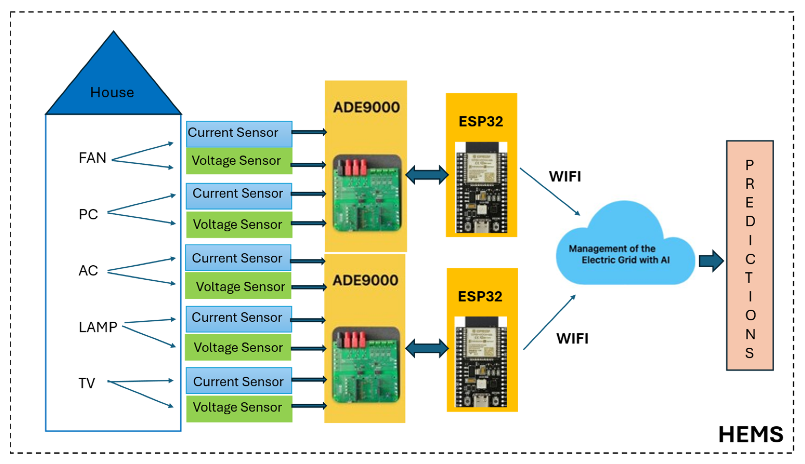
Home energy management systems (HEMS) are technological solutions designed to intelligently monitor, manage, and optimize energy consumption in homes. These platforms integrate smart meters and a controller to monitor and optimize the energy consumption of devices used in the home. The main goals of HEMS are to reduce energy costs, lower environmental impacts, and improve home comfort. By providing detailed data and management tools, these systems facilitate informed decision-making and the adoption of more sustainable energy consumption habits [4]. However, traditional HEMS often rely on reactive data analysis rather than predictive approaches, which limits their ability to optimize energy use efficiently. To make the best decisions and consequently improve the efficiency of these HEMS, predictive algorithms are required to provide accurate data on the future behavior of energy consumption and appliance usage time.

Artificial intelligence is a branch of computer science that seeks to create systems that are capable of performing tasks which normally require human intelligence and plays an important role in improving the efficiency of these systems. Machine learning (ML), a sub-discipline of AI, focuses on the development of algorithms and models that enable computers to learn, make predictions, and make data-driven decisions [5,6]. Deep learning is a machine learning technique that uses multi-layered artificial neural networks to learn the hierarchical representations of data, allowing the hierarchical learning of data representations. This approach has proven to be highly effective in a variety of applications, including energy-related applications [5,6]. Advanced deep learning methods such as recurrent neural networks with long short-term memory (LSTM) are being implemented to optimize energy consumption, providing accurate predictions of energy usage [7].

Traditional methods for forecasting energy consumption and device usage time, such as ARIMA models or linear regressions, have several limitations. These approaches often have difficulty capturing nonlinear and complex patterns in time series data and often fail to provide accurate predictions due to their inability to handle high temporal variability. In addition, traditional HEMS with inaccurate predictions cannot effectively optimize energy use. Therefore, an LSTM model is proposed to address these shortcomings by learning nonlinear relationships and long-term dependencies, which is ideal when working with time series data such as energy consumption data, which can have patterns that vary throughout the day, week, or even month, thus improving accuracy and efficiency in energy management. This predictive capability allows for the anticipation of energy demand, enabling proactive decision-making to prevent unnecessary consumption and improve household energy efficiency.

The novelty of this research lies in integrating an LSTM model to predict both energy consumption and appliance usage time in HEMS. Unlike previous approaches, which primarily focus on real-time monitoring, this study leverages historical data from smart meters to enhance predictive accuracy and optimize energy management. By enabling better demand forecasting, this approach supports energy efficiency, reduces unnecessary consumption, and lowers greenhouse gas emissions. Additionally, it promotes sustainable consumption habits and facilitates the integration of renewable energy sources in households, contributing to sustainability goals.

This LSTM-based model used to predict the individual and total energy consumption and the usage time of different household devices has the main function of estimating or anticipating the future behavior of energy consumption and appliance usage time based on patterns learned from historical data. The LSTM neural network can process past data inputs and predict future values. This makes it possible to anticipate, for example, how much energy an appliance will consume at a specific time, providing a valuable tool for efficient energy planning and management in the home.

2. Related Work

The long short-term memory (LSTM) networks are a type of recurrent neural network (RNN) specifically designed to handle data sequences and address the vanishing gradient problem typically associated with traditional RNNs. LSTM networks achieve this with a unique structure composed of cells, input gates, output gates, and forgetting gates, which allow them to maintain long-term dependencies more effectively than standard RNNs. These networks are particularly efficient in time series prediction, natural language processing, and other applications that require the modeling of temporal sequences [8,9]. According to Khosravani et al. (2016), Liu et al. (2019), and Wei et al. (2019) [10,11,12], these advanced deep learning techniques (LSTM) are being implemented to optimize energy consumption by providing accurate predictions of energy usage.

LSTM networks have proven to be particularly effective in predicting energy consumption [10]. They have been used in models to predict energy consumption in smart buildings, achieving high accuracy and efficiency in predictions [11,12]. These advanced deep learning techniques allow for the optimization of energy consumption, providing accurate predictions of energy use [13,14]. Moreover, compared to other algorithms, LSTM networks prove to be more effective in predicting energy consumption due to their ability to handle data sequences and retain long-term information. In recent studies, it has been observed that LSTM-based models outperform other methods, such as traditional deep neural networks (DNNs) and traditional regression models, in terms of accuracy and ability to adapt to complex energy consumption patterns.

Table 1. Comparison of related works.

Model	Description	Applications	Challenges	References
LSTM	Captures long-term dependencies.	Time series forecasting, complex dependencies.	High computational cost, long training time.	[15]
Bi-LSTM	Bidirectional LSTM for better context capture.	Sequences with past–future dependencies.	Increased complexity and training time.	[14]
Stacked LSTM	Multiple LSTM layers for deeper feature extraction.	Complex time series modeling.	Higher computational cost.	[16]
GRU	Simplified LSTM with fewer parameters.	Faster training, good temporal dependencies.	May be less accurate in some cases.	[17]
Bi-GRU	Bidirectional GRU for improved accuracy.	Past–future dependencies in sequences.	More computationally expensive.	[18]
Stacked GRU	Multi-layer GRU for advanced features.	Complex time series.	Increased training time.	[19]
ARIMA	Uses autoregression and integration for stationary data.	Works well for clear patterns.	Not suited for complex dependencies.	[20]
SARIMA	ARIMA with seasonal adjustment.	Forecasting seasonal trends.	Parameter tuning complexity.	[21]
Prophet	Handles seasonality automatically.	Easy to use, good for multi-seasonal data.	Less customizable.	[22]
XGBoost	Boosted trees for accuracy.	Handles nonlinear relationships.	High computational demand.	[23,24]

summarizes the most relevant features of some related works.

According to the reviewed works, long-term memory recurrent neural networks (LSTM) stand out as the best choice for home energy applications due to their ability to handle long sequences and capture complex temporal dependencies. LSTM is particularly effective in short- and long-term electrical load forecasting, where time variations and seasonal behavior are critical. Studies such as that of [25] have shown that LSTM-based models, especially when combined with attention mechanisms, provide superior accuracy in electrical load forecasting. Some recent studies have also explored the combination of LSTM with Generative Adversarial Networks (GANs) as an alternative approach to enhance prediction capabilities by generating synthetic training data. While promising, these hybrid models require further validation to determine their practical advantages in real-world energy management applications [26].

In addition, the LSTM architecture allows for the integration of multiple layers (stacked LSTM), which further enhances the model’s ability to capture the abstract and complex features of the data, as observed in research by [16]. For these reasons, LSTM provides a robust and efficient solution for managing and forecasting energy consumption in home environments.

3. Description of the HEMS

The developed HEMS consists of four components: home-use devices, smart meters, a dataset, and an AI module. Typical home devices are connected to individual smart meters that calculate how much energy each of these devices consumes in kWh, allowing for the detailed monitoring of energy consumption. The dataset includes historical energy consumption information, which is fed to the AI module, allowing the model to analyze and learn from the relevant consumption information. Finally, the AI module, which is the brain of the HEMS, is responsible for processing and analyzing the data collected from home devices to make predictions, incorporating a prediction algorithm that analyzes historical consumption data to make future projections of the energy consumption and usage time of appliances. The smart meters used for this research have been developed and tested at the Manglar Laboratory, a research laboratory of the Department of Electronic Engineering at the University of Sucre. Figure 1 shows the structure of the developed HEMS to collect energy consumption data. These meters were built using five SCT013-000 (Beijing YaoHuadechang Electronic Co., Ltd., Beijing, China) non-invasive current transformer (CT)-type current sensors, designed to measure an alternating current (AC) without interrupting the electrical circuit, five ZMPT101B voltage sensors (Shenzhen, China) designed for measuring an alternating current (AC) voltage in a safe and isolated manner (one sensor each per device), and two ADE9000 (Analog Devices, Inc., Wilmington, MA, USA) and two ESP32 (Espressif Systems, Shanghai, China), distributed among the five devices. The ADE9000 is a high-precision multi-phase energy meter designed for power quality monitoring, compliant with various standards such as IEC 61000-4-30, IEC 61000-4-7, IEC 62053-21, IEC 62053-22, IEC 62053-23, and IEC 62053-24. It features an SPI communication interface and four pulse outputs for connection to external devices. This device features seven high-performance analog-to-digital converters (ADCs), a digital integrator, a temperature sensor, a voltage reference circuit, and a waveform buffer. It also incorporates embedded algorithms to accurately calculate multiple electrical variables. The ESP32 is a high-performance microcontroller with Wi-Fi and Bluetooth connectivity, designed for IoT applications and embedded systems. In this case, the ESP32 acts as a bridge between the ADE9000 and the intelligent management system in the HEMS, receiving current and voltage data, processing it, and sending it via Wi-Fi to a cloud platform with AI to optimize energy use.

4. Materials and Methods

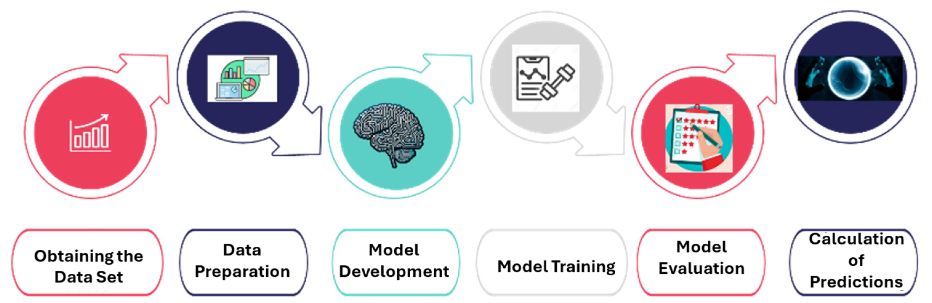
The methodology encompasses data collection and preparation, model development, training, and evaluation. The focus is on transforming consumption data into a time series to fit and validate a predictive model that can provide accurate estimates for home energy management. Figure 2 shows these steps, which are then explained in detail.

4.1. Obtaining the Dataset

The data used for this study were collected from a typical household located in Sincelejo, Colombia. A typical home in Colombia is defined as a middle-class household with access to the national electricity grid, with a standard single-family dwelling structure and equipped with common appliances such as a computer, television, fan, air conditioning, and an energy-efficient lighting system, among others. It is inhabited by a family of four: a homemaker, a school-age child, a health statistician, and an older adult. This represents an energy consumption pattern aligned with the common work and household dynamics of the study’s target population. This structure allows for the analysis of energy consumption patterns that reflect typical residential use in the area, considering both the length of time the dwelling has been occupied and the consumption habits of its inhabitants.

This characterization provides context for the implementation of the HEMS and ensures that the results obtained are representative of a typical residential environment in Colombia and that the dataset reflects a realistic residential scenario.

The data collected include a time sequence of energy usage measurements on the 5 devices recorded at one-hour intervals. These data were collected to identify consumption patterns throughout the day for 12 months. Each record represents a consumption value and is linked to a specific moment in time, following a chronological order; this characteristic which identifies time series allows for the analysis and modeling of consumption patterns over time. The dataset is organized into 8785 rows corresponding to the header row and the recorded data, and 6 columns distributed as shown in

Table 2. Data set summary.

Timestamp	Fan	PC	AC	Lamp	TV
2/01/2024 0:00	0.0160	0	0.2149	0.0002	0.0002
2/01/2024 1:00	0.0161	0	0.3141	0.0000	0.0001
2/01/2024 2:00	0.0160	0	0.2156	0.0000	0.0001
2/01/2024 3:00	0.0160	0	0.2459	0.0000	0.0002

. It is important to clarify that although the total number of hours expected in a standard year is 8760 (24 × 365), the dataset contains 8784 records, this being because 2024 is a leap year. The additional 24 h correspond to February 29th, which adds one more day to the dataset.

4.2. Data Preparation

The data preparation process makes the data suitable for model training, allowing the model to learn and make predictions about time series with greater accuracy. This process starts by exploring the data to observe how they are organized and structured, and to identify particularities such as the identification of outliers or null values, which includes identifying outliers, handling missing values, and formatting timestamps. This division ensures a robust evaluation of the model’s performance.

The dataset was divided into three subsets:

• Training set: 70% of the data (6150 records)
• Validation set: 10% of the data (878 records)
• Test set: 20% of the data (1756 records)

Time format adjustment is performed by converting the original time series into a format suitable for training the LSTM model.

Specifically, a sliding window is used to create the input sequences (X) and the corresponding outputs (Y), where each input contains look_back previous steps, and the output is the next value of the time series (predicted value). For this study, we initially used a one-hour retrospection window (look_back = 1), which provides immediate adaptability for short-term energy management. This reformatting process is achieved by the create_dataset function. The purpose of adjusting the time format is to transform the data from a one-dimensional series to a set of input–output pairs that the LSTM model can process. This allows the model to learn the temporal dependencies in the data and make predictions based on historical patterns.

The next step is the normalization or scaling of the data; for this, the model uses the MinMaxScaler object from the sklearn.preprocessing library. Normalization scales the time series values to a range between 0 and 1. Normalization helps to reduce the variance in the data, which facilitates the model’s learning process and prevents large values from dominating the cost function, which facilitates model training and improves model performance. Next, the time window size and the prediction size are determined. The selection of the time window size (look_back) defines how many previous time steps are considered as inputs to predict the next value. The size of the predictions refers to how many time steps into the future the model is designed to predict. For this case, the time window takes one previous time step and performs a one-step prediction (one step into the future). The one-step prediction allows the model to make more accurate short-term forecasts, since immediate dependencies are usually stronger and easier to model. Since the size of the time window is 1 and the size of the predictions is also 1, and the dataset provides hourly consumption, the model predicts consumption for the next hour. In other words, the model uses the last hour’s energy consumption to predict the energy consumption and device usage time for the next hour after the last data entry in the dataset.

The normalized time series are then transformed into input (X) and output (Y) sequences, where each input sequence contains a defined number of previous time steps and the output sequence contains the future values to be predicted. This process is performed by a function that runs through the data and creates sliding windows, where each window of look_back size becomes an input sequence and the next value in the series becomes the corresponding output. By using sliding windows, the model can capture how past values influence future values, allowing the model to learn patterns and temporal dependencies in the data.

The data preparation process also includes the calculation of individual consumption and time of use. To calculate the individual consumption, we have the energy consumption data of the different devices. Then, a segment of the normalized data (energy values) is taken which corresponds to the prediction period (time window of the normalized data). This segment is stored in a list (y_energy). These values will be the ones that the model will try to predict. They are like “correct answers” for the model to learn. The usage time can be deduced from the consumption pattern; it is calculated by how much time the device has been used in a specific period, and this information is used to help the model learn. For this, the sum of the energy consumption in a specific time window is calculated; this value is repeated to match the number of predictions it is making. These values are stored in another list (y_usage_time).

Finally, the X and y_energy lists are converted into NumPy arrays, and this step ensures that the data are compatible, efficient, and easy to manipulate during the whole training and evaluation process of the model.

4.3. Model Development

LSTM recurrent neural networks were used for model development due to their ability to handle long-term dependencies in sequential data. Prior to the normalization process, the data are split; the data-splitting process involves separating the original dataset into two subsets: one for training and one for testing. This step is performed with the train_test_split function of the sklearn.model_selection library. The training subset (70% of the data) is used to train the machine learning model. During this process, the model learns patterns and relationships in the data. The test subset (30% of the data) is used to evaluate the performance of the model once it has been trained. This allows the measurement of the model’s ability to generalize and make accurate predictions on new and unpublished data.

The implemented model is a single LSTM neural network with a bifurcated architecture. A single input layer is used, indicating that both predictions share the same initial data representation. The network is then split into two specialized branches: one for predicting energy consumption and the other for usage time. This bifurcation allows the network to learn task-specific features without losing consistency in the initial data representation.

The use of this structure is justified because, although device energy consumption and usage time are related, they exhibit distinct patterns that can benefit from specialized LSTM layers. If a single output were used for both predictions, the ability to capture these distinct patterns would be lost. At the same time, by sharing the input layer, consistency in the representation of the input data is maintained.

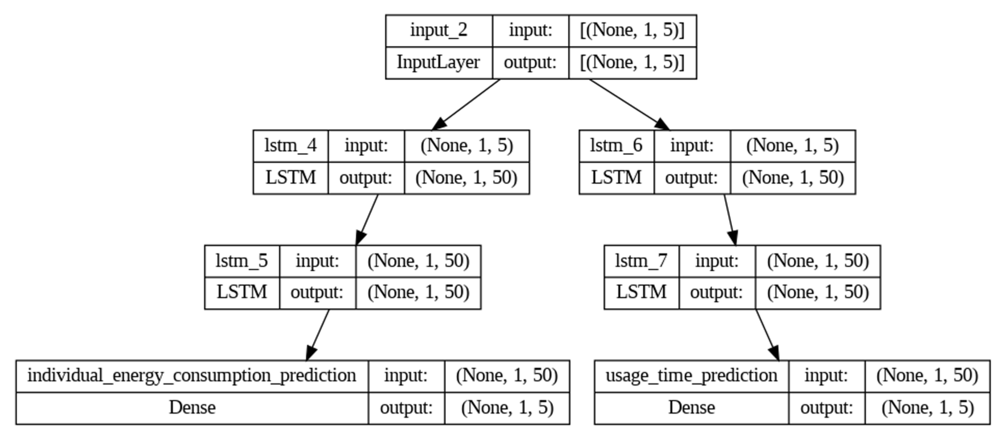
This model has been structured with 4 LSTM layers (2 for consumption and 2 for time of use) and 2 dense layers, 1 for consumption and 1 for the time of use for each appliance in the dataset. Figure 3 shows the structure of the model.

The model is built using the sequential class of Keras, which allows the stacking of layers sequentially. This allows the building of a linear architecture in which one layer follows another. The first layer of the model is the input layer, which organizes and transforms the data into the appropriate format for the LSTM to process time sequences, allowing the model to learn and predict patterns in the time series data. The input layer configuration ensures that the model receives the data in the correct format to process the time series. The inputs are the variables used to make the predictions; in the case of this model, the inputs are the measurements of energy consumption in kWh of the 5 devices recorded at 1 h time intervals. The input layer of an LSTM must receive the data in a three-dimensional format, with dimensions that include the number of samples, where each sample is a time window, the number of time steps, which is the length of the time window (window_size), and the number of features, which are the variables that describe each time step (such as energy consumption).

The next layers of the model are LSTM layers. LSTM layers are capable of learning long-term dependencies in data streams. These layers handle time series and other data sequences where historical context is important for future predictions. Each of the 4 LSTM layers uses 50 LSTM units, which represent the number of memory cells in the layer. In these layers, the ReLU (Rectified Linear Unit) is used as a trigger function to introduce nonlinearities into the model, and the input form specifies the size of the time window (n_steps) and the number of features (n_features). Following the LSTM layers, a dense layer is incorporated for consumption prediction and one for time of use. Dense layers are fully connected layers in which each neuron is connected to all neurons in the previous layer. That is, each dense layer performs the final regression to predict either energy consumption or usage time, with 1 unit of output each. As an activation function, the dense layers use the linear function suitable for the nature of the outputs, which are continuous predictions of energy consumption and time of use, as it simply returns the value of the input.

Finally, it is possible to detail the 3 types of layers in the model as follows:

• Input layer (input_2): Input layer with shape (None, 1, 5). This means that the input data are expected to have a variable size (None) with a time sequence of length 1 and 5 features (energy consumption of the five appliances).
• LSTM layers (lstm_4, lstm_6, lstm_5, lstm_7): These are the LSTM layers that process the temporal sequences. Each layer has a shape output (None, 1, 50), indicating that it produces a temporal sequence of length 1 with 50 features. The parameter numbers are 11,200 for the first LSTM layers and 20,200 for the second ones due to the higher complexity and number of connections.
• Dense layers (individual_energy_consumption_prediction and usage_time_prediction): These are dense layers (fully connected) that produce the final predictions. Each layer has a shape output (None, 1, 5), corresponding to the individual energy consumption and usage time predictions for the five appliances. Each layer has 255 trainable parameters.

Table 3. Layer details.

Layer	Type	Output Shape	Parameters	Connections
input_2	InputLayer	(None, 1, 5)	11,200	[‘input_2[0][0]’]
lstm_4	LSTM	(None, 1, 50)	11,200	[‘input_2[0][0]’]
lstm_6	LSTM	(None, 1, 50)	11,200	[‘input_2[0][0]’]
lstm_5	LSTM	(None, 1, 50)	20,200	[‘lstm_4[0][0]’]
lstm_7	LSTM	(None, 1, 50)	20,200	[‘lstm_6[0][0]’]
Individual Energy Consumption Prediction	Dense	(None, 1, 5)	255	[‘lstm_5[0][0]’]
Usage Time Prediction	Dense	(None, 1, 5)	255	[‘lstm_7[0][0]’]

summarizes and details the layers of the LSTM model designed to predict the energy consumption and usage time of household appliances.

Finally, the model is compiled; the compilation process in Keras combines the optimizer and the loss function to prepare the model for training, using the ADAM (Adaptive Moment Estimation) optimizer and the MSE (mean squared error) loss function to train the model. The optimizer is used to update the model weights efficiently and effectively during training, and the loss function provides a measure of how well the model makes predictions compared to the actual values, thus guiding the process of adjusting the model parameters to minimize this error.

4.4. Model Training

Model training is the stage where the neural network adjusts its parameters (weights and biases) from the training data, using an iterative adjustment process based on the prediction error. This process allows the neural network to learn patterns from the training data, adjusting its parameters to improve predictions. This iterative process optimizes the model so that it can make accurate predictions on unseen data, evaluating its performance with validation data to ensure good generalization.

In this case, model training is performed using X_train, which are the energy consumption sequences, and the labels y_train_energy and y_train_usage_time, which represent individual energy consumption and appliance usage time, respectively. The model is trained for 50 epochs (epochs = 50), using batches of 32 samples per iteration (batch_size = 32). In total, 10% of the training data is separated for validation (validation_split = 0.1), and the data are not shuffled between epochs (shuffle = False) to maintain temporal sequentiality. Figure 4 shows the training process.

During training, the model processes batches of 32 energy consumption sequences, generating predictions for individual consumption and time of use. The MSE loss function calculates the error between these predictions and the actual values. Using the Adam optimizer, the model adjusts its weights and biases to minimize this error. This adjustment is performed after each batch of data and is repeated throughout the 50 training epochs. At the end of each epoch, the model is evaluated using 10% of the training data reserved for validation, which helps to monitor its generalization ability and to detect possible overfitting.

4.5. Model Evaluation

Model evaluation ensures that the model’s performance is not only measured during training but also validates its ability to generalize to previously unseen data. This process begins by evaluating it on test data that it has not seen before, using the evaluation method to calculate the mean squared error (MSE). This error value is printed to understand the performance of the model. Then, loss records are extracted during training and validation, which are plotted to visualize how the losses changed over time. This allows us to see if the model learned correctly and if there are signs of overfitting or underfitting. Figure 5 shows the model’s evaluation process.

4.6. Calculation of Predictions

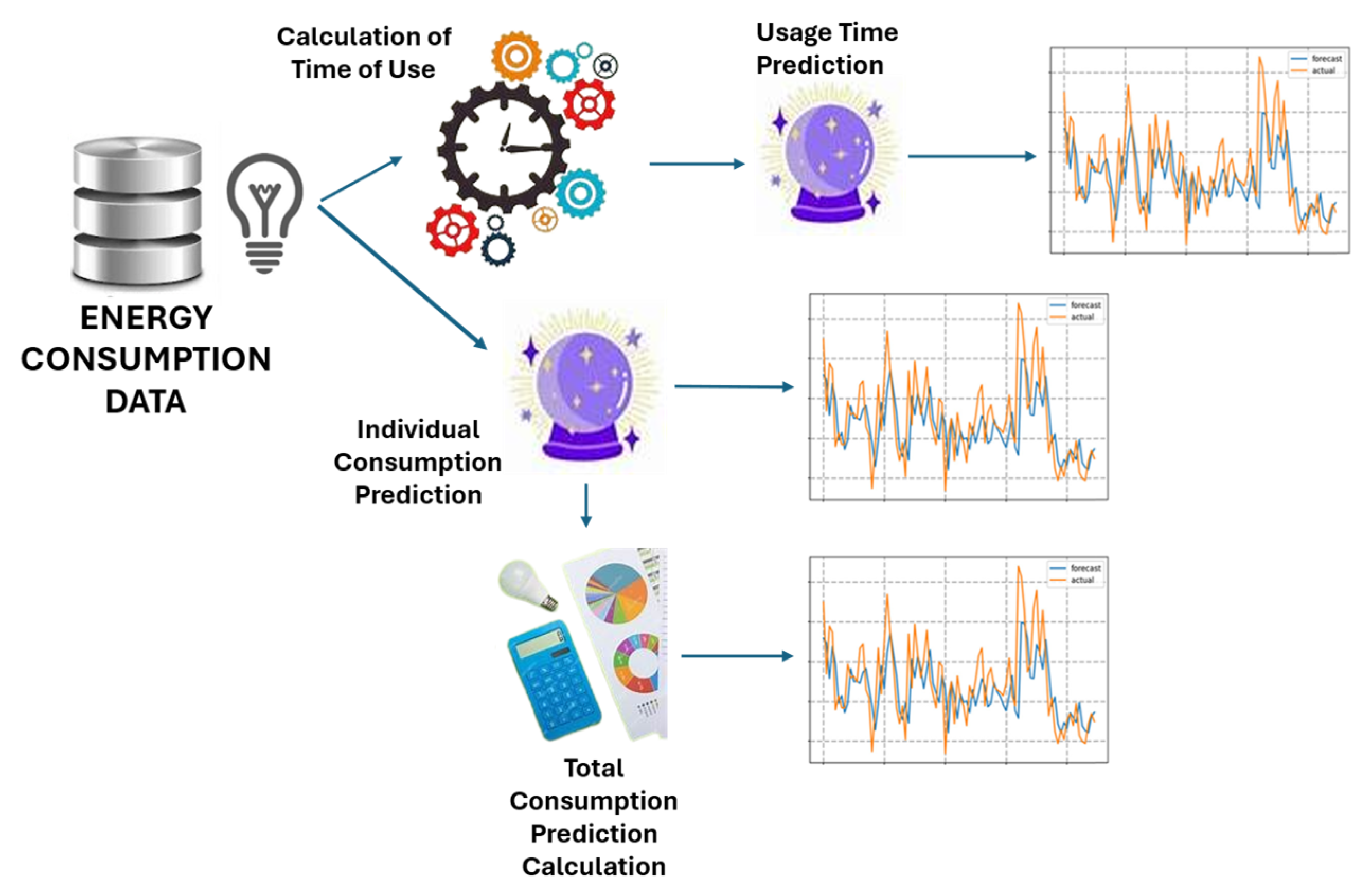
The ultimate goal of the model is to make predictions of the energy consumption and time of use of typical household devices. The model provides predictions of disaggregated and total consumption and the predictions of usage time, as shown in Figure 6.

• Calculation of individual consumption and time-of-use predictions: After training the model, it is used to predict new data that it has not seen before, such as the test set (X_test), applying what it has learned during training to make the predictions. The model makes two types of predictions: one for individual appliance energy consumption and one for appliance usage time. To make predictions with a model in Keras, the predict function is used; the predict function takes the input data X_test and returns the model’s predictions. In this case, since the model has two outputs (one for energy consumption and one for usage time), the predict function predicts two arrays: y_pred_energy for energy consumption and y_pred_usage_time for usage time. This process allows the model to make predictions on new data. This step ensures that the model produces results that can be used to evaluate its performance and compare them with actual values. The predictions obtained can then be compared with actual test data to calculate performance metrics (MSE, for example) and validate the accuracy of the model.
• Calculation of total consumption predictions: Finally, the actual and predicted total energy consumption are calculated and then compared to understand if the model is making good predictions relative to the actual data. To accomplish this, first, the actual total energy consumption at each time point is calculated by taking the consumption of all appliances in a time window and averaging them. Then, the same is performed with the total consumption predicted by the model for those same points in time. These results are then compared to verify how well the model reflects the actual pattern of energy consumption. Sum functions are used to sum up the data and flatten the results in a single dimension. Having the total consumption predictions allows for the evaluation of whether the model correctly captures the overall consumption trends, not only for each appliance individually but as a whole.

The described methodology provides a complete framework for the implementation of an LSTM model in the prediction of energy consumption and device usage time. This approach allows verifying the accuracy of the model and its ability to capture consumption patterns, facilitating a more efficient energy management adjusted to the real needs of the household.

5. Results and Discussion

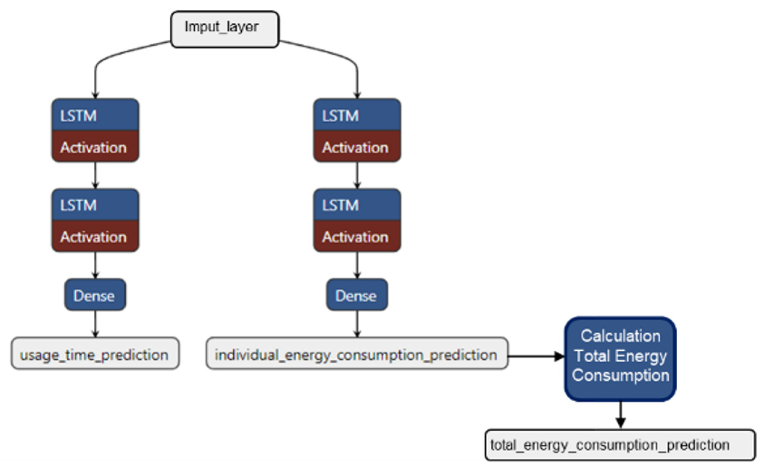
This section presents the results obtained from the prediction model developed. The analysis includes the evaluation of the model’s performance and the comparison between actual data and predictions. The complete structure of the prediction model is illustrated in Figure 7, providing a detailed view of the components and data flow within the model. This figure represents the architecture of the LSTM network-based model for total energy consumption prediction. The model consists of two main branches that work in parallel to predict device usage time (usage_time_prediction) and individual energy consumption (individual_energy_consumption_prediction). Each of these branches consists of two LSTM layers followed by an activation layer and a dense layer (Dense), which allows for the better capturing of temporal dependencies in the energy consumption and usage time data. The predictions from both branches are then combined to calculate the total energy consumption (total_energy_consumption_prediction). The model uses a stacked LSTM architecture, meaning that multiple LSTM layers are employed sequentially. The rationale for this configuration is to improve the model’s ability to learn complex patterns in time series. The first LSTM layer extracts basic features from the input sequence, while the second LSTM layer refines this information and captures more abstract relationships between the data. This approach improves the model’s accuracy in predicting energy consumption and device usage time, resulting in more robust estimates for energy management in domestic environments.

This model can predict energy consumption over a given period. The number of days predicted depends on the size of the time window, the size of the predictions, the prediction method used, and the availability of historical data. In this case, the combination of these factors allowed the model to predict 2635 h, equivalent to approximately 110 days of energy consumption.

To determine how many hours the model predicted, we can compare the number of rows in the training dataset to the number of rows in the prediction file. The training dataset contains 8784 rows of data, while the prediction file has 2635 rows of data. Each row in the prediction file represents one hour of predicted energy consumption, which means that the model predicted 2635 h of energy consumption. Converting these hours to days, we find that the model predicted approximately 109 days of energy consumption (2636 h ÷ 24 h/day ≈ 109.791 days).

The HEMS model developed in this research has yielded very good results in predicting the energy consumption and usage time of household appliances, which will allow users to better plan their domestic activities and optimize energy consumption in the home. Using LSTM networks, the model achieved significant accuracy in predicting energy consumption patterns from historical data, proving to be able to identify and forecast future energy demands with high accuracy.

The performance of the HEMS model was evaluated using a test dataset, using the model.evaluate() method, and the loss history during training was plotted. The results show that the total loss metric (loss) is 0.0168, the loss for individual energy consumption_prediction_loss (individual_energy_consumption_prediction_loss) is 0.0168, and the loss for usage_time_prediction_loss (usage_time_prediction_loss) is 4.8922 × 10⁻⁷. The evaluation of the model on the test set yielded a total mean squared error (MSE) of 0.0168, this being the same value for the individual energy consumption prediction, while the MSE for the usage_time_prediction_loss was 4.8922 × 10⁻⁷. On a scale of 0 to 1, an MSE close to zero is ideal, indicating very accurate predictions. Specifically, an MSE below 0.1 is considered very good, between 0.1 and 1 could be acceptable depending on the context, and above 1 indicates high discrepancies requiring improvement. The results obtained with a total MSE and for the individual energy consumption prediction of 0.0168 demonstrate high model accuracy. In addition, the extremely low loss and MSE for time-of-use prediction reinforce the model’s excellent ability to capture energy consumption patterns, indicating robust and reliable overall performance for home energy management applications.

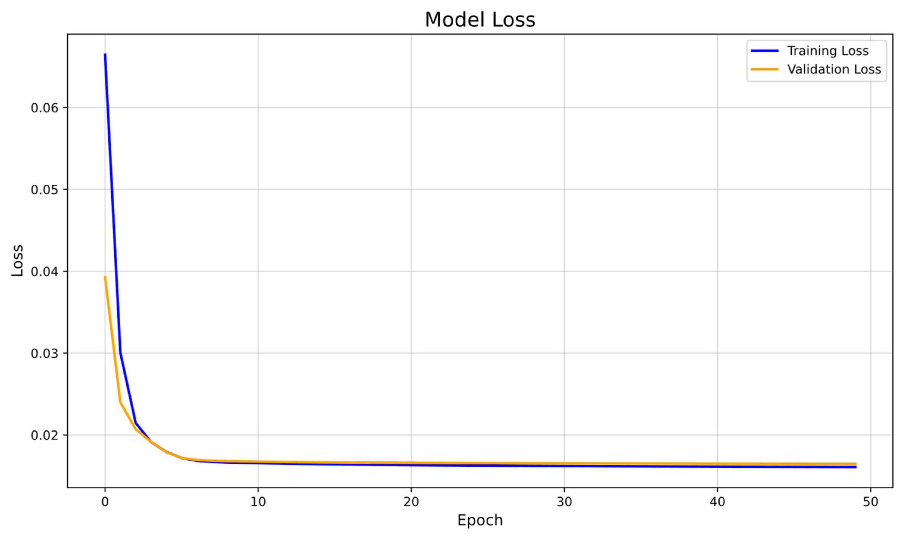
Figure 8, entitled “Graph of Loss during Training”, shows how the model loss, in terms of mean squared error (MSE), varies over time during the training process. In this graph, the vertical (y) axis represents the loss, while the horizontal (x) axis shows the number of epochs. The blue line in the graph reflects the loss in the training set, and the yellow line reflects the loss in the validation set. This graph allows us to understand the learning of the model and to detect possible cases of overfitting. In the developed model, a continuous decrease in the loss in both the training and validation sets is observed as the epochs progress. This suggests that the model is learning effectively and generalizing correctly to unseen data, with no evidence of overfitting. This ability of the model to keep losses low in both sets indicates good performance for predicting the energy consumption and appliance usage time in the home.

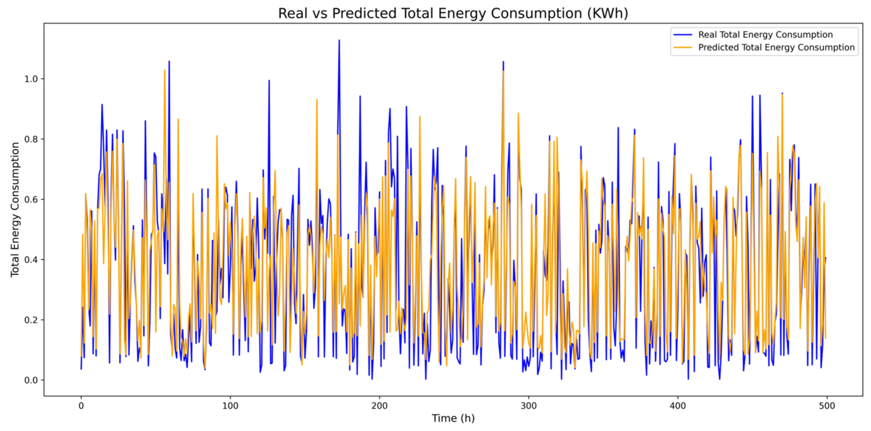
In evaluating the model’s predictions, graphs have been generated that show a comparison between the actual values and predictions of energy consumption over time, providing a clear and detailed view of its performance. The purpose of these graphs is to visualize and evaluate the accuracy of the model predictions compared to the actual values. If the orange and blue lines are close to each other, it means that the model performs well in prediction. These comparisons have been made for each appliance’s energy consumption, usage time, and total consumption. Figure 9 shows the energy consumption predictions: (a) fan, (b) PC, (c) air conditioner (AC), (d) lamp, and (e) TV. Figure 10 presents the usage time predictions in the same order: (a) fan, (b) PC, (c) AC, (d) lamp, and (e) TV. Finally, Figure 11 shows total consumption.

These comparative time series graphs demonstrate remarkable accuracy in the predictions; in particular, the lines representing the actual values and the predictions align closely, highlighting the effectiveness of the model in most cases. Figure 6, illustrating the appliance usage time, is particularly noteworthy, showing an almost perfect match between predictions and actual values; the lines are so similar that the graph tends to unify into a single color. This level of accuracy not only underscores the model’s success in predicting usage time but also highlights its overall ability to accurately capture energy consumption patterns. These results confirm the robustness of the model in the prediction task, which generates support for applications and improvements in the analysis of energy consumption behavior.

Additionally, a detailed analysis has been performed with various evaluation metrics to evaluate the performance of the LSTM model, using the metrics mean squared error (MSE), mean absolute error (MAE), root mean squared error (RMSE), and coefficient of determination (R²); these typical regression loss functions are defined as follows:

$$MSE={\displaystyle \frac{1}{n}}\sum _{i=1}^n{\left(y_i-{\widehat{y}}_i\right)}^2$$

$$MAE={\displaystyle \frac{1}{n}}\sum _{i=1}^n\left|y_i-{\widehat{y}}_i\right|$$

$$RMSE=\sqrt{{\displaystyle \frac{1}{n}}\sum _{i=1}^n{\left(y_i-{\widehat{y}}_i\right)}^2}$$

$$R^2=1-{\displaystyle \frac{{\sum }_{i=1}^n{\left(y_i-{\widehat{y}}_i\right)}^2}{{\sum }_{i=1}^n{\left(y_i-{\overline{y}}_i\right)}^2}}$$

where

• $n$: Total number of observations in the dataset.
• $y_i$: Real or true value of observation i.
• ${\widehat{y}}_i$: Value predicted by the model for observation i.
• $\overline{y}$: Mean or average of actual values, ($\overline{y}={\displaystyle \frac{1}{n}}\sum _{i=1}^n{y}_i$).

Evaluations are performed both at the individual appliance level and at the global level to obtain a complete perspective of the performance.

Table 4. Error metrics by device for individual energy consumption and time of use.

Appliance	Type	MSE (kWh2)	MAE (kWh)	RMSE (kWh)	R2
Fan	Energy	0.00034	0.01141	0.01849	0.7704
	Usage	9.40 × 10−6	0.0658	0.0969	0.9999
PC	Energy	0.00001	0.00143	0.00357	0.5930
	Usage	9.55 × 10−9	0.00238	0.00309	0.9995
AC	Energy	0.02251	0.09347	0.15003	0.6518
	Usage	0.00154	0.00098	0.00124	0.9999
Lamp	Energy	0.00003	0.00398	0.00547	0.4513
	Usage	9.24 × 10−9	0.00222	0.00304	0.9998
TV	Energy	0.00017	0.00783	0.01298	0.6874
	Usage	5.74 × 10−7	0.0178	0.0240	0.9999

shows the evaluation for each appliance.

As shown in Table 4, the model presents high accuracy in the prediction of usage time with minimum errors and an R² close to 1, indicating that the model has a very good fit to the data; this shows an excellent correspondence between predicted and actual values. In contrast, energy consumption shows greater variability between appliances, with higher MSE and RMSE values, especially for air conditioning. However, these values are still acceptable.

Table 5. Overall error metrics for individual energy consumption and time of use.

Metrics	Energy Consumption	Time of Use
$\mathrm{MSE}(\mathrm{k}\mathrm{W}{\mathrm{h}}^2$)	0.00461	3.10 × 10−4
$\mathrm{MAE}\left(\mathrm{k}\mathrm{W}\right)$	0.02362	0.00021
R2	0.82566	0.99999

shows the overall evaluation of the model, taking the predictions of individual energy consumption and time of use together.

As seen in Table 5, the overall evaluation shows that the model has excellent performance in predicting usage time, with an R² close to 1 and very low errors. For energy consumption, although the errors are higher, they are still quite low, and the R² is very close to one, indicating a good ability of the model to fit the predictions to the real data.

Table 6. Metrics for total energy consumption.

Metrics	Value
$\mathrm{MSE}(\mathrm{k}\mathrm{W}{\mathrm{h}}^2$)	0.00093
$\mathrm{MAE}\left(\mathrm{k}\mathrm{W}\mathrm{h}\right)$	0.01926
$\mathrm{RMSE}\left(\mathrm{k}\mathrm{W}\mathrm{h}\right)$	0.03044
R2	0.65620

shows the metrics for total energy consumption, i.e., the consumption of the five devices.

The evaluation of total consumption shows an overall good performance of the model, with low MSE, MAE, and RMSE, and an R² indicating an acceptable ability to fit the predictions to the actual total consumption. The results confirm that the model is effective in predicting the total energy consumption for all appliances combined.

The results of the evaluation metrics for the full model are presented in

Table 7. Error metrics for the full model.

Metrics	Value
$\mathrm{MSE}(\mathrm{k}\mathrm{W}{\mathrm{h}}^2$)	0.00461
$\mathrm{MAE}\left(\mathrm{k}\mathrm{W}\mathrm{h}\right)$	0.02384
$\mathrm{RMSE}\left(\mathrm{k}\mathrm{W}\mathrm{h}\right)$	0.06847
R2	0.91282

, i.e., the individual and total energy consumption and the time of use of the five devices.

The overall evaluation of the full model highlights robust performance on all key metrics. The MSE and MAE are relatively low, and the R² is high, indicating that the model has an excellent ability to capture both the energy consumption and time of use in an overall context.

The model shows high accuracy in the prediction of appliance usage time, with extremely low MSE and MAE values and an R² close to 1. This suggests that the model effectively captures the temporal behavior of usage. For energy consumption, although the errors are higher compared to the time of use, the results are still good and show a good level of fit with the energy consumption predictions. The overall model evaluation and the total consumption evaluation also highlight the model’s ability to capture global dynamics with remarkable accuracy.

The results obtained confirm that the LSTM model has achieved outstanding performance in predicting the energy consumption and time of use of household appliances. The graphs and metrics indicate a high accuracy and fitting capability, especially in the prediction of time of use, where the matches between predictions and actual values are almost perfect. This prediction’s success reinforces the effectiveness of the model in practical energy management applications and provides a solid basis for future optimizations and improvements.

Furthermore, to ensure the practical applicability of the model in an HEMS, we analyzed the impact of different lookback window sizes (1, 12, and 24 h) on prediction accuracy; we then compared them in

Table 8. Comparison with different time windows.

Time Window	MSE (kWh2)	MAE (kWh)	RMSE (kWh)	R2	Processing Time (s)
1 h	0.00461	0.02384	0.06847	0.91282	72.61
12 h	0.00469	0.02391	0.06850	0.63541	291.75
24 h	0.00472	0.02395	0.06853	0.750230	476.49

.

While a longer lookback period could capture broader consumption patterns, our results indicate that increasing the window size does not significantly improve model accuracy and actually increases the processing time. The selected 1 h window offers the best balance between accuracy and computational efficiency, allowing users to make timely adjustments to their energy consumption, achieving practical utility and computational efficiency in the context of an HEMS.

Additionally, to evaluate the performance of the proposed LSTM model, a comparison was implemented with a simple reference model, known as the Naïve Model or persistence model. This model is not a neural network or a machine learning algorithm but rather a baseline strategy that assumes that the energy consumption and usage time of devices in a given hour will be the same as those of the previous hour. The Naïve Model is widely used in data science as a benchmark because it does not perform pattern learning or parameter tuning, it relies solely on the continuity of historical data, and it allows for the verification of whether a more complex model, such as the LSTM, actually improves prediction.

For the comparison, the LSTM model was trained using historical energy consumption and device usage time data, and its performance was evaluated alongside the Naïve Model using standard metrics: MSE, MAE, RMSE, and R².

Table 9. Comparison of the developed model with a reference model.

Model	MSE (kWh2)	$\mathbf{MAE}\left(\mathbf{k}\mathsf{\omega }\right)$	$\mathbf{RMSE}\left(\mathbf{k}\mathsf{\omega }\right)$	R2
Naïve Model	0.00682	0.03173	0.08263	0.31174
LSTM	0.00461	0.02384	0.02384	0.91282

shows this comparison.

The results indicate that the LSTM model significantly outperforms the baseline model across all metrics. The LSTM’s MSE, MAE, and RMSE are considerably lower, suggesting more accurate predictions; the LSTM’s R² coefficient is 0.6562, while the Naïve Model’s is 0.3117, meaning that the LSTM better explains the variability in the data. These findings demonstrate that the LSTM model not only improves prediction accuracy but also better captures underlying patterns in device energy consumption and usage time, outperforming the simple approach based on historical data persistence.

Finally, a comparison of the developed model against models developed by other authors has been carried out, and

Table 10. Comparison of the developed model against models developed by other authors.

Article	Proposed Model	Technique Used	Metrics Reported	MSE (kWh2)	MAE (kWh)	RMSE (kWh)	R2	Energy Consumption Prediction	Device Usage Time
[16]	CNN + LSTM	Hybrid	MAE, MSE, RMSE	0.0877	0.1565	0.1485	NA	Moderate accuracy	Not detailed
[27]	LSTM	Neural Networks	NA	NA	NA	NA	NA	Limited in long-term prediction	Not detailed
[17]	LSTM	Machine Learning	MAE, RMSE, R2	NA	0.0583	0.0837	0.7337	Good accuracy	Not detailed
[17]	GRU	Machine Learning	MAE, RMSE, R2	NA	0.0621	0.0873	0.7067	Good accuracy	Not detailed
[17]	DROP-GRU	Hybrid	MAE, RMSE, R2	NA	0.0574	0.0813	0.7482	Moderate accuracy	Not detailed
[28]	LSTM	Deep Learning	MSE, MAE	0.002	0.0297	NA	NA	High precision	Not detailed
[29]	LSTM	Machine Learning	NA	NA	NA	NA	NA	Good accuracy	Not detailed
[30]	LSTM	Neural Networks	NA	NA	NA	NA	NA	Acceptable prediction	Partially detailed
[31]	CNN_BiLSTM	Neural Networks	MSE, MAE, RMSE, R2	0.45	0.046	0.67	0.91	High accuracy	Partially detailed
[32]	LSTM	Machine Learning	MSE, MAE, RMSE	0.0317	0.1350	0.1780	NA	Moderate accuracy	Not detailed
[33]	LSTM	Deep Learning	MSE, MAE, RMSE	0.1654	0.2662	0.4067	NA	Acceptable accuracy	Not detailed
[34]	LSTM	Deep Learning	MSE	NA	NA	NA	NA	High precision	Not detailed
[35]	GWO-LSTM	Hybrid	MSE, MAE	0.09	0.06	NA	NA	Moderate accuracy	Not detailed
[36]	DNN	Deep Learning	MSE, MAE	NA	NA	NA	NA	High accuracy	Not detailed
[37]	LSTM	Deep Learning	NA	NA	NA	NA	NA	High accuracy	Partially detailed
Developed Model	LSTM (Unidirectional)	Deep Learning	MSE, MAE, RMSE, R2	0.0046	0.0236	0.0684	0.91	High accuracy in high variability scenarios	Accurate and detailed

shows this comparison.

A comparison of different energy consumption prediction models shows that the developed model, based on a one-way LSTM, offers significant advantages in terms of accuracy and applicability in high-variability scenarios. Unlike other models, such as those based on CNN + LSTM, GRU, or GWO-LSTM, the developed model exhibits the lowest error rate (MSE = 0.0046, MAE = 0.0236, RMSE = 0.0684) and a coefficient of determination R² of 0.91, indicating a high capacity for generalization and data fitting.

Compared to other evaluated LSTM models, many lack reported metrics or show higher error values. For example, models such as the LSTM from [28] and the CNN_BiLSTM from [31] show higher error values or less detailed predictions. Additionally, the energy consumption prediction in most of the reviewed models does not consider device usage time, which limits their applicability in home energy management systems (HEMS). In contrast, the developed model incorporates this information accurately and in detail, making it a more robust and adaptable option to consumption scenarios with high variability.

Finally, it can be said that the incorporation of a one-way LSTM model with a low error rate and a detailed focus on device usage time offers a more accurate and reliable solution compared to other approaches previously reported in the literature.

Based on the results obtained, it is possible to perform an analysis that allows the detection of patterns of both energy consumption and usage time for each of the devices on the test bench. These patterns can then be used to optimize energy consumption by implementing strategies that allow the modification of habits, the optimization of loads, or the programming of the use of devices, among others.

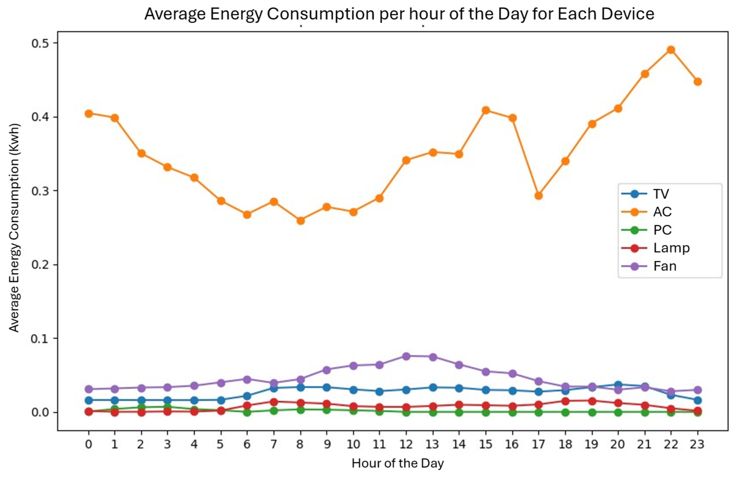
Figure 12 shows a line graph that represents the variations in the average energy consumption (kWh) of the five appliances over 24 h of the day, allowing the consumption of each of them to be compared. The X axis represents the time of day, and its scale goes from 0 to 23, representing each hour of the day. The Y axis represents the average consumption (kWh), and its scale goes from 0 to approximately 0.5. The air conditioner is represented by the orange line and has values between 0.25 and 0.5 kWh, the fan is represented by the purple line and has values between 0.02 and 0.1 kWh, the TV is represented by the blue line and has values between 0.01 and 0.05 kWh, the PC is represented by the green line, and the lamp is represented by the red line; these last two have similar values that are below 0.02 kWh. As can be seen, it is possible to deduce which devices have a higher consumption. The AC has the highest line, with higher consumption at night and a decrease in the early morning; the fan has a stable consumption with a slight increase between 10 am and 2 pm; the TV, PC, and lamp have low consumption with a slight increase in the afternoon and evening. This pattern indicates which devices should be prioritized in optimization strategies, such as scheduling their use or operating them at specific times.

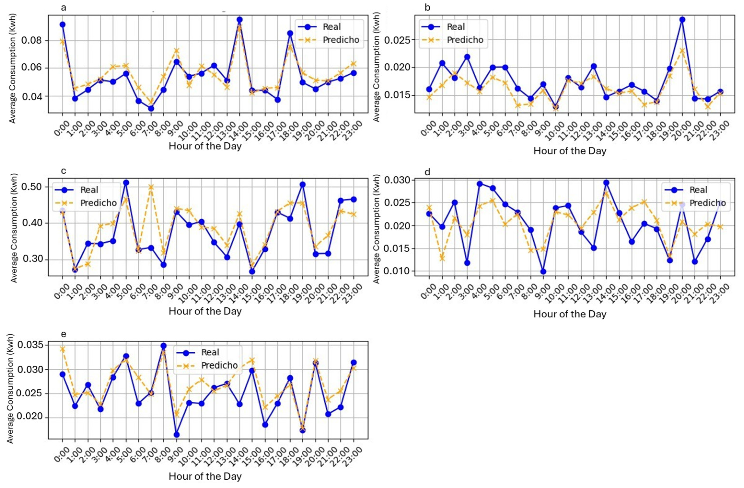
Figure 13 shows the behavior of the usage time patterns of each of the five real and predicted devices for a typical day. Figure 13a—average daily fan pattern, Figure 13b—average daily PC pattern, Figure 13c—average daily air conditioning pattern, Figure 13d—average daily lamp pattern, and Figure 13e—average daily TV pattern. The analysis of these patterns allows us to detect device usage habits that produce peaks in consumption and, based on the results, modify the habits to optimize the consumption of the devices.

To analyze the average daily behavior across all available data, the daily average energy consumption (kWh) was calculated for each device and plotted over 24 h. This allows for an understanding of how energy consumption is distributed throughout a typical day. The calculated hourly average provides insights into the general consumption pattern over all recorded days.

In addition to these examples, these consumption and usage time patterns can be analyzed by days of the week or hours of the day, which can help schedule the use of the devices at specific times based on, for example, the availability of renewable energy.

6. Challenges and Limitations

Despite the strong predictive performance achieved, several technical and operational challenges arose during the development of the system. One of the main technical challenges was the optimization of the model’s hyperparameters, as fine-tuning these parameters significantly impacted prediction accuracy. Multiple adjustments were required to achieve the observed improvements in the graphical comparisons and to minimize error metrics, ensuring stable and reliable predictions. Additionally, structural modifications to the model architecture were necessary. Initial inconsistencies and dimensionality errors in the layers led to prediction instability, which was mitigated by refining the layer configuration, ultimately improving model convergence and efficiency.

From an operational perspective, while the system has demonstrated effectiveness in its current test environment, its scalability to a larger number of households and a broader range of devices per household remains an area for future investigation. Expanding the dataset to include diverse household energy consumption behaviors would provide further validation of the model’s robustness and adaptability. Moreover, incorporating real-time deployment in actual smart home environments would allow for the testing of its performance under dynamic conditions, assessing aspects such as data transmission latency, computational efficiency, and integration with different home energy management platforms.

7. Conclusions

The increase in household electricity consumption, driven by technological advances and the increased time people spend indoors, has generated the need for systems that monitor and reduce this consumption. In this context, home energy management systems (HEMS) have gained popularity, especially with the use of artificial intelligence to improve their accuracy and efficiency.

This study proposes a model based on LSTM networks to predict individual and total energy consumption, as well as the usage time of five household devices connected to an HEMS. The results obtained demonstrate the model’s predictive accuracy: for individual consumption, the model achieves an MSE of 0.0168, an MAE of 0.0294, and an RMSE of 0.1296, with an R² of 0.82566, confirming its high predictive capacity. However, there is some variability between devices, with the air conditioning exhibiting the highest error (MSE = 0.02251); however, this error remains relatively low. For total consumption, the model maintains an MSE of 0.00093, an MAE of 0.01926, and an RMSE of 0.03044, ensuring a reliable prediction at the global level. For time-of-use prediction, the model achieves an extremely low MSE of 4.8922 × 10⁻⁷ kWh², with R² values close to 1 across all devices, reflecting a near-perfect correlation between predicted and actual values. The overall performance of the model is validated by its overall R² of 0.82566, indicating that it effectively captures consumption patterns despite small variations between appliances. Error metrics indicate high reliability, with low MSE (0.00461), MAE (0.02384), and RMSE (0.06847) values for the full model. These results confirm an excellent correlation between actual and predicted values and demonstrate the model’s suitability for predicting energy consumption and device usage time.

To evaluate its relative effectiveness, the LSTM model was compared to a benchmark Naïve Model. The results show that the Naïve approach produces significantly higher errors, with an MSE of 0.00682, a MAE of 0.03173, and an RMSE of 0.08263, demonstrating the superior predictive accuracy of the proposed LSTM model. Furthermore, the R² of the Naïve Model remains at 0.31174, while the LSTM model achieves R² values above 0.91, highlighting its ability to model energy consumption trends more accurately. Compared to alternative architectures such as hybrid GRU + CNN and CNN + LSTM models, the proposed one-way LSTM model achieves comparable accuracy with lower computational costs. Hybrid models often exhibit MSE values around 0.0183–0.0201 for individual consumption and 0.00105–0.00112 for total consumption, which are close to the performance of LSTMs. However, these approaches tend to present a higher risk of overfitting and greater computational demand, making the LSTM-based approach a more efficient and scalable solution for real-world HEMS applications.

Predicting both the energy consumption and usage time of devices within an HEMS represents an approach that significantly improves prediction accuracy and consumption optimization. This not only optimizes energy usage but also offers new opportunities for the intelligent scheduling of household activities and cost reductions on electricity bills.

8. Future Work

Although positive results have been obtained in this research, there are several opportunities to improve and expand the HEMS model. Increasing the dataset, incorporating more appliances and scenarios, as well as considering climatic and seasonal factors, could strengthen the robustness and generalizability of the model. Integrating real-time data would allow immediate decisions on energy use, while analyzing the economic and environmental impact would help quantify the benefits of the technology. It is also important to include active control functions to optimize the performance of appliances, along with security and privacy measures that protect user information. Additionally, as part of future research, the integration of Building Information Modeling (BIM)-based methodologies could be explored to improve the energy management of smart homes. BIM allows for the modeling of the structure and the operation of buildings by integrating additional contextual data (e.g., building structure and thermal properties), which could complement energy predictions by incorporating detailed information about the physical environment and its interaction with devices. This LSTM model has proven to be effective and provides a basis for future innovations that could transform energy management in the home, promoting sustainability and energy efficiency in line with the global goals of emissions reduction and resource conservation.