Article

Experimental Investigation of Wind Effect on Roof Configurations with Photovoltaic Panel Systems for Sustainable Building Design

by
Răzvan-Andrei Polcovnicu
1,
Sebastian-Valeriu Hudișteanu
1,*,
Nicolae Ţăranu
1,2,3,
Dragoș Ungureanu
1,2,
Marius Alexa
1,
Iuliana Hudișteanu
1,
Cătălin Onuțu
1 and
Alexandru-Florin Mustiață
1
1
Faculty of Civil Engineering and Building Services, Technical University “Gheorghe Asachi” of Iasi, 67 Prof. D. Mangeron, 700050 Iasi, Romania
2
The Academy of Romanian Scientists, 3 Ilfov Street, Sector 5, 050663 Bucharest, Romania
3
Technical Sciences Academy of Romania, 26 Dacia Blvd., 030167 Bucharest, Romania
*
Author to whom correspondence should be addressed.
Sustainability 2025, 17(10), 4739; https://doi.org/10.3390/su17104739
Submission received: 16 April 2025 / Revised: 16 May 2025 / Accepted: 20 May 2025 / Published: 21 May 2025
(This article belongs to the Special Issue Harnessing Renewable Energy: A Sustainable Path to Carbon Neutrality)

Abstract

:
This study investigates the aerodynamic behavior of roof structures under wind-induced forces, focusing on buildings equipped with photovoltaic panels. Experimental data were obtained through wind tunnel testing of three 1:100 scale models, each representing a distinct roof geometry: gabled, hipped, and multi-pitched. Measurements of dynamic pressure and pressure coefficients were conducted for various wind incidence angles, ranging from 0° to ±150°. The results highlight the impact of roof geometry and PV panel placement on the pressure distribution, with notable variations due to flow separation and vortex formation around the panels. Gabled roofs exhibited pronounced pressure gradients, while hipped roofs showed more uniform distributions. Multi-pitched roofs demonstrated the most complex aerodynamic behavior due to their variable slopes. These findings enhance the understanding of wind-structure interactions for buildings with roof photovoltaic panels, contributing to the development of more resilient and energy-efficient structures. The research supports sustainable construction practices by improving wind load predictions and informing design decisions that promote the safe integration of renewable energy systems into the built environment.

1. Introduction

The integration of rooftop photovoltaic (PV) panel systems has become increasingly prevalent as the global energy sector shifts toward renewable sources. Rooftops of existing and newly constructed buildings provide a practical platform for implementing solar energy systems, optimizing otherwise underutilized surfaces. For pitched roofs, especially on existing structures, stand-off mounting methods are widely used, where PV modules are installed above the roof surface using structural supports [1,2]. However, these systems introduce significant aerodynamic complexity, which remains insufficiently explored in current literature.
Recent studies have shown that rooftop-mounted PV panels are highly susceptible to wind-induced loads, particularly uplift and suction forces, which can threaten their structural integrity during high wind events [3,4,5]. Experimental and numerical investigations emphasize that the presence of PV panels modifies the boundary layer flow, promotes vortex formation, and alters pressure distributions, especially near panel edges and roof eaves [6,7,8]. Wind tunnel studies [9,10,11,12] have demonstrated that peak pressure coefficients on tilted PV panels can significantly exceed those on bare roofs, raising critical design concerns.
Previous studies [6,10] identified substantial pressure variations caused by rooftop PV installations, particularly at roof edges and panel corners. Our results confirm these observations by showing that peak uplift forces tend to occur near the rear edges of panels on pitched and complex roofs. Moreover, the experimental data reinforce conclusions drawn by Aly and Rone [9], who reported that tilted panel installations intensify aerodynamic loading due to flow separation. Despite the growing number of studies in this domain [13], comprehensive comparative analyses between various roof geometries under consistent experimental conditions remain scarce. This gap hinders the development of standardized design solutions for PV systems on complex rooftops.
Understanding the wind behavior around rooftop PV systems is essential for their safe and reliable deployment. Wind loads not only impact structural safety but also influence panel lifespan, energy performance, and long-term maintenance costs. Current design standards, such as Eurocode 1 and ASCE 7-22, provide general guidance for wind actions on structures but often lack detailed prescriptions for roof-mounted PV arrays, especially on non-flat or irregular roofs [14].
Furthermore, lightweight building structures—frequently used in residential and modular construction—are particularly vulnerable to wind uplift when PV systems are installed. This underscores the importance of accurately quantifying pressure coefficients for varied roof geometries to improve resilience under extreme wind events [15].
This study contributes to sustainable construction practices by providing experimental data that improve the safety, resilience, and performance of rooftop PV systems. The results are relevant for engineers and designers aiming to create buildings that are both energy-efficient and structurally robust, aligning with the goals of climate-resilient and sustainable urban development.
The novelty of this research lies in the experimental investigation of three distinct roof geometries—gable, hip, and multi-pitched—each equipped with PV panel systems, tested under consistent wind tunnel conditions. By capturing pressure distributions at various wind incidence angles, the study offers new insights into complex wind-structure interactions specific to PV-equipped sloped roofs.
The main objective of this work is to analyze and compare dynamic pressure coefficients on different pitched roof configurations with PV systems, thereby improving wind load estimation and informing safer, more efficient rooftop solar designs.

2. Theoretical Background and Basis for Calculations

2.1. Fundamental Equations for Wind Pressure Analysis

Dynamic pressure represents the kinetic energy per unit volume of wind and is essential for understanding the forces exerted on a surface. It plays a crucial role in structural engineering by estimating the wind loads acting on building components such as roofs, facades, and walls [16].
pd = 0.5 ρ v2
where pd represents the dynamic pressure [Pa], ρ denotes the air density [kg/m3] (Air density can be considered 1225 kg/m3 in standard conditions), and v is the wind velocity [m/s].
To account for variations in pressure distribution across different roof geometries, dynamic pressure coefficients are employed. These dimensionless coefficients express the ratio of actual wind pressure on a surface to the reference dynamic pressure [17]:
c v = p p d
where cv characterizes the dynamic pressure coefficient, p is the wind pressure on a given surface [Pa], and pd represents the reference dynamic pressure [Pa].
Pressure coefficients provide a fundamental means of assessing wind-induced loads and are highly sensitive to factors such as roof geometry, surface roughness, and orientation relative to wind direction [18].

2.2. Aerodynamic Principles of Wind-Structure Interaction

A deeper understanding of wind-structure interactions, particularly for roofs with externally mounted PV panels, requires consideration of key aerodynamic principles. One of the most fundamental is Bernoulli’s principle, which states that within a steady, incompressible flow, an increase in wind velocity results in a decrease in pressure. This principle helps explain how variations in wind speed across a roof surface generate pressure differentials [7].
When wind encounters obstacles such as roofs or photovoltaic panels, the airflow tends to separate from the surface, creating turbulence and vortices [19]. These phenomena cause significant pressure variations, especially in the wake regions behind the panels, which can influence both structural integrity and performance [18].
Additionally, the boundary layer, defined as the thin region of air near the roof surface where viscous effects are significant, is affected by the presence of PV panels. These panels alter the characteristics of the boundary layer, increasing turbulence and modifying wind speed and pressure distribution on the surface [9].
The turbulence and wake effects caused by PV installations are further intensified by increased surface roughness. Panel tilt angle, orientation, and arrangement influence wake dynamics, generating non-uniform aerodynamic behavior across the roof and contributing to complex and asymmetric pressure distributions [10].

2.3. Effect of Roof Geometry on Wind Pressure Distribution

Roof geometry significantly influences how dynamic pressure is distributed on a building’s surface. Traditional aerodynamic models typically classify roofs as either flat or pitched, with pressure coefficients obtained through experimental data. However, the introduction of photovoltaic panels complicates these models by introducing additional airflow disturbances that affect the aerodynamic response.
For flat roofs, wind tends to impact the surface perpendicularly, resulting in a relatively uniform pressure field. However, the addition of PV panels alters this behavior by creating localized flow disturbances. These disruptions lead to pressure variations, particularly on the leeward side of the panels, where turbulence develops and suction forces may increase [6,20].
In the case of pitched roofs, both the angle of inclination and the wind direction play major roles in determining how pressure is distributed along the windward and leeward faces. The installation of PV panels on such roofs further complicates airflow behavior by enhancing turbulence and modifying the existing pressure patterns. Variables such as panel tilt, spacing, and alignment relative to the roof slope can either amplify or mitigate these aerodynamic effects [10].
Understanding these effects is very important, especially for lightweight roofs, which are more prone to failure under unbalanced uplift forces.

2.4. Empirical Models and Experimental Data

Empirical models estimate dynamic pressure coefficients based on wind tunnel experiments and real-world data. These models incorporate variables such as roof geometry, wind direction, and surface roughness to approximate wind forces. However, existing models primarily focus on standard roof designs and often overlook complexities introduced by PV panels [21].
Wind tunnel experiments remain essential in refining empirical models. By simulating different wind conditions and measuring resulting pressures on various roof and PV configurations, researchers improve pressure coefficient accuracy. These studies enhance structural load predictions, leading to more reliable design methodologies [10,22,23]. Despite these advancements, empirical models still lack calibration for PV-equipped pitched roofs, creating uncertainty in load estimation.

2.5. Implications for Structural Design

The theoretical aspects discussed have significant implications for designing buildings with externally mounted PV panels. The aerodynamic alterations introduced by PV systems require new design standards that account for these changes. Accurate wind pressure prediction is essential for ensuring roof structural integrity while optimizing energy performance [24].
A thorough understanding of wind behavior around PV-equipped roofs enables engineers to develop more resilient structures that withstand wind forces while maintaining long-term sustainability. The presence of PV panels on building roofs presents both challenges and opportunities, requiring an advanced theoretical framework based on fluid dynamics, aerodynamic drag, and empirical data to inform future research and design advancements [25,26].
However, both Eurocode 1 [14] and ASCE 7-22 [27] provide only general guidance for wind loads on building surfaces and lack specific criteria for pitched roofs with elevated PV systems. This absence leads to uncertainty in design, especially when accounting for complex geometries and varying panel tilt angles. Recent critiques in the literature also highlight that the conservative simplifications used in current codes may result in either underestimation or overestimation of actual uplift forces [9,21]. This reinforces the need for wind tunnel data under controlled conditions to supplement existing code provisions.

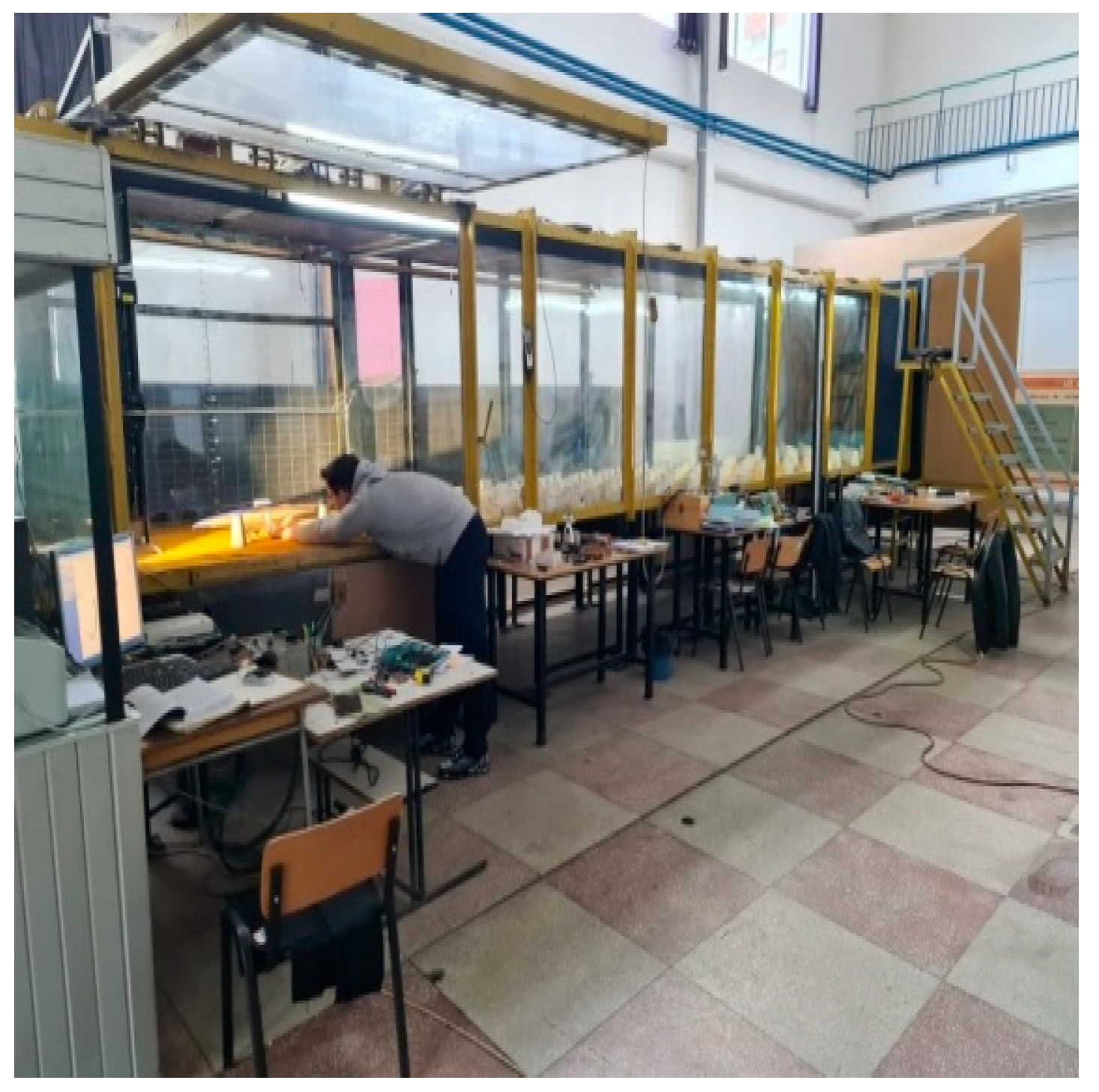
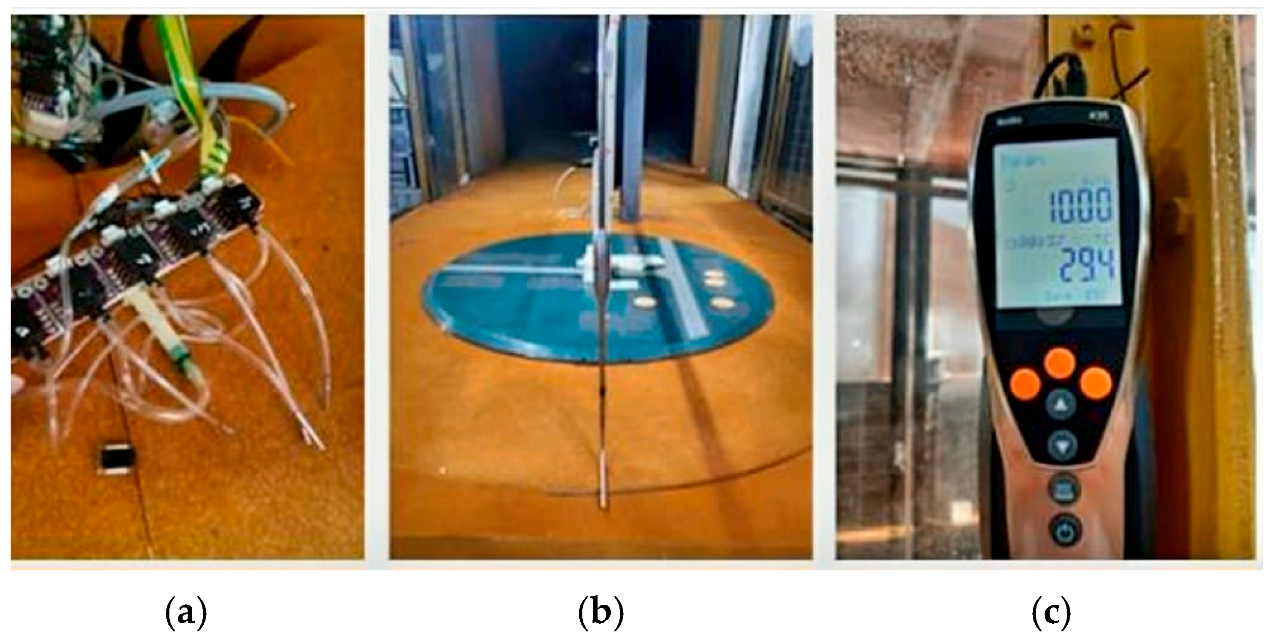
3. Experimental Setup and Measurement Methodology

The experiments conducted in this study to determine the dynamic pressure coefficients and dynamic pressures on rigid roof models with photovoltaic panel systems were carried out in the Building Aerodynamics Laboratory, part of the Department of Civil and Industrial Construction at the Faculty of Civil Engineering and Installations, “Gheorghe Asachi” Technical University of Iași (Figure 1). To perform the experiment and evaluate the predefined parameters, including measuring the velocities and average pressures necessary to determine the mean pressure coefficients on the studied models, the following specialized equipment, shown in Figure 2, was used: an anemometer, TESTO 435 digital anemometer, hot-wire anemometric probes from TSI Incorporated, headquartered in Shoreview, Minnesota, differential micromanometer, Pitot tube, pressure taps and connecting tubes, and an alcohol manometer.
The measurement of fluctuating pressures on rigid models, which allows for the determination of mean values, peak pressure coefficients, and standard deviations, was conducted using the specialized experimental equipment illustrated in Figure 2. To capture and store the data obtained during testing, a combination of software tools was employed. LABVIEW and LABWINDOWS were used for data acquisition and processing, generating files with the .DAT extension compatible with DOS-WINDOWS operating systems. Subsequently, dedicated programs were utilized to convert these files into binary format (.BIN) and to perform corrections and statistical analysis on the recorded data. All instruments and procedures were selected based on international wind engineering best practices and in line with recommendations from EN 1991-1-4 [14] and relevant aerodynamic testing protocols [28].

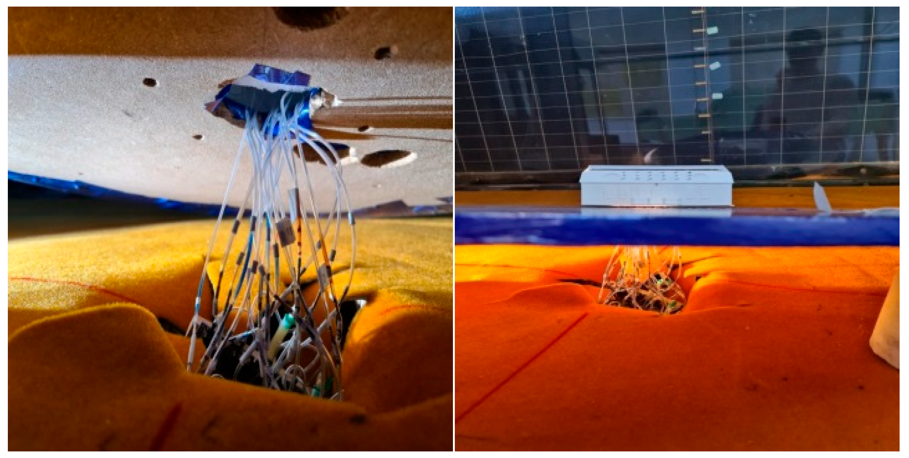
3.1. Local Pressure Measurement Protocol

The pressure measurement approach followed established methods commonly used in wind tunnel testing of architectural models [14,28]. Where applicable, standard relationships and calibration steps were applied to ensure reproducibility and accuracy. In the aerodynamic tunnel, static and total pressures are measured using a Pitot tube, which is securely positioned in the direction of airflow. This setup enables the accurate determination of the reference wind velocity, a key parameter in the evaluation of dynamic pressure. The appropriate height for taking pressure and velocity measurements is selected based on the geometric proportions of the model being tested, ensuring that the Pitot tube is aligned with the model’s effective reference height.
Once positioned, the Pitot tube provides direct readings for both the total pressure (pt0) and the static pressure (ps0) at the reference point. With these values, the dynamic pressure (pd0) is calculated as the difference between total and static pressure, as expressed by the following relation [14]:
pd0 = pt0ps0
The pressures on the surface of the models were measured using pressure transducers, positioned according to the principle of systems that collect data from multiple pressure ports. The pressure changes applied to both sides of the transducer membrane are detected electrically, using capacitive or inductive methods, or through micro-comparators. The transducers used in the aerodynamic tunnel on models are connected via a system of tubes to the pressure ports.
The process of installing and measuring local pressures on the wind-exposed surface of the model begins with the mounting of the pressure transducer. This device is affixed to the model’s surface, oriented perpendicularly to the direction of wind flow to accurately capture pressure fluctuations. The installation height is selected based on the mean velocity profile corresponding to the simulated atmospheric boundary layer, ensuring consistent reference conditions across all measurements. The transducer placed at this position provides reference data essential for interpreting the pressure distribution.
Following installation, the terminals of the pressure transducers are connected to the terminal block of the data acquisition board, as illustrated in Figure 3. This setup allows for the synchronized signal transmission from the pressure taps to the recording system, enabling precise tracking of aerodynamic effects during testing.
The data acquisition board is connected to a computer system to facilitate the digital recording of measured values. The recording and monitoring process is managed using LABVIEW Signal Express software, which enables real-time data visualization, storage, and subsequent processing.
Local pressure measurements obtained at various points on the surface of the model—denoted as point i—are used to compute the corresponding local aerodynamic coefficients. These are expressed through the following relation [9]:
c p i = p i p s p t p s
where c p i represents the dynamic pressure coefficient at point i, p i is the measured dynamic pressure at point i on the tested model [Pa], ps is the static pressure [Pa], and pt is the reference total pressure measured in the airflow region [Pa].
This dimensionless coefficient provides a normalized measure of wind-induced pressure relative to the reference dynamic conditions, offering a basis for comparing aerodynamic behavior across different roof geometries.
To ensure the accuracy of the recorded data, two preliminary correction procedures were conducted before initiating the actual measurements. The first correction involved measuring the pressure using a Pitot tube positioned at the reference height, upstream of the model. This step provided initial values for total pressure (pt1) and static pressure (ps1), establishing a baseline for the airflow conditions within the tunnel.
In the second step, the total pressure was measured again at the same reference height, but this time at the precise location where the model would be placed, while the model itself was absent. This measurement yielded a second pair of values, namely pt0 for total pressure and ps0 for static pressure, representing the undisturbed airflow conditions at the intended test location. These values served as calibration references to correct for any spatial variability in pressure within the wind tunnel.
These correction steps are crucial to compensate for potential variations in the measurement environment and to ensure the accuracy and reliability of the data obtained during the experiment.
Although, in theory, static pressure should remain constant, in practice, small differences are observed in the wind tunnel along the airflow direction. To correct these discrepancies and ensure data coherence, correction factors are determined in accordance with the specifications provided. This is done by applying relations (5) and (6) [21]:
c p s = p s 1 p s 0 p t 0 p s 0
where c p s represents the differential correction for static pressure, p s 1 is the static pressure measured at a point in the wind tunnel [Pa], p s 0 is the reference static pressure [Pa], and p t 0 is the reference total pressure [Pa] [21].
γ = p t 0 p s 0 p t 1 p s 1
where γ is the correction factor, p t 1 represents the total pressure measured at a point in the tunnel [Pa], p s 1 is the static pressure measured at the same point [Pa].
The corrections can be integrated directly into the aerodynamic coefficients according to the relation (7) [29]:
c p i = 1 γ p i p s 1 p t 1 p s 1 + Δ c p s
where c p i is the corrected pressure coefficient, p i represents the pressure measured at the point of interest [Pa], and Δ c p s is the differential correction of the static pressure.
Before beginning the actual test sequence, each sensor’s signal output was individually verified using a manual air pump. This verification ensured that all sensors and pressure transducers responded correctly to sudden variations in pressure, confirming their operational sensitivity and the absence of signal lag or faults in the system.
Following this verification step, the Pitot tube was securely mounted in its designated position within the wind tunnel and connected to the pressure transducers. With the system fully assembled, instantaneous pressure values generated by the wind at a specific point k on the model’s surface were recorded over a given time interval t. These measurements enabled the calculation of local aerodynamic coefficients at each point, based on the corresponding reference pressure values. The reference pressure was determined using the established reference wind speed, in accordance with applicable aerodynamic standards.
The aerodynamic coefficients obtained through this process are statistical in nature, representing time-averaged quantities that characterize the wind’s interaction with the model surface. These values are essential for evaluating pressure distributions and aerodynamic loads across the roof configurations tested. These procedures were followed uniformly for all tested configurations to ensure consistency and allow comparative analysis across the roof geometries.
The mean value of the pressure coefficient at a given point k on the surface of the model was determined using the time-averaged pressure measured during the test interval. This average value, denoted as c ¯ p k , is calculated according to Equation (8), which relates the mean pressure to the dynamic pressure derived from the reference wind speed [10]:
c ¯ p k = p ¯ k 1 2 ρ u ¯ r e f 2
where c ¯ p k represents the mean pressure coefficient, p ¯ k is the mean pressure at point k [Pa], ρ defines the air density [kg/m3], and u ¯ ref characterizes the reference average wind speed [m/s].
The standard deviation of the pressure coefficient, also referred to as the root mean square of the pressure fluctuations, is calculated using Equation (9). This parameter quantifies the magnitude of pressure variation around the mean value at point k, providing insight into the unsteady aerodynamic behavior at that location [10]:
c p k = p k ( t ) p ¯ k ¯ 2 1 2 ρ u ¯ r e f 2
where c p k is the standard deviation of the pressure coefficient, p k ( t ) expresses the instantaneous pressure measured at point k at time t [Pa], and p ¯ k characterizes the mean pressure at point k [Pa].
The experimental procedure began with the careful positioning of the model on the rotating platform inside the wind tunnel. Initially, the model was oriented perpendicularly to the airflow to ensure uniform exposure across its surface. Once the setup was verified, the access door of the wind tunnel was closed and securely fastened to eliminate any external disturbances during the test.
Before activating the motor, an initial set of pressure readings was taken at each pressure tap while the wind speed was set to zero. This baseline measurement established a reference point for subsequent dynamic comparisons. Following this step, the electric motor was gradually powered up, and the airflow velocity was increased in controlled increments—typically between 1 and 2 m/s—until the predetermined test speed was reached.
Once steady-state conditions were achieved, the data acquisition system was activated, and pressure values at all ports were recorded at a high sampling frequency. The first complete set of fluctuating pressure data was captured over a defined interval, generally lasting 30 s, and stored for later analysis and interpretation.
Subsequently, the model was repositioned on the rotating platform to simulate different wind incidence angles. For each new orientation, a fresh series of pressure measurements was recorded, allowing the researchers to evaluate variations in pressure distribution due to changes in wind direction.
Following the completion of the testing sequence, the motor speed was gradually reduced until the wind tunnel came to a complete stop, thereby marking the end of the experiment.

3.2. Data Acquisition and Processing Procedure

The data collected from the pressure taps were statistically processed using established signal analysis techniques adapted from Bendat and Piersol [23], ensuring accurate calculation of mean values and dynamic pressure coefficients. To process the data obtained from the laboratory tests conducted in the wind tunnel, a structured methodology was applied, involving several distinct stages. The total number of pressure taps installed on the three roof models—M1, M2, and M3—was denoted by k, ranging from 1 to 19, including the Pitot tube channel.
At time zero, with the wind tunnel motor turned off and wind speed set to zero, the signal was collected from all pressure taps and the Pitot tube. For each pressure tap k, the signal was recorded over a time interval T of 30 s, resulting in 30,000 samples denoted as uik1, …, uik30,000. Later, at a time ti, with the wind speed increased to a predefined testing level, the signal from each pressure tap on the models was recorded again over the same 30 s interval, generating a new set of 30,000 samples: ukm, where k = 1 …30,000 and m = 1 …30,000.
To correct the raw data, the mean offset for each pressure tap was first calculated using Equation (10) [28]:
u ¯ k o =   u ¯ k 1 + +   u ¯ k 30,000 30,000
Subsequently, the corrected signal values were obtained by subtracting this mean offset from the corresponding measurement taken during motor operation at the test speed, as shown in Equation (11) [28]:
u k m c o r = u k m   u ¯ k o
Once the corrected signal values were established, statistical analysis was performed to derive the relevant parameters. The first step involved calculating the arithmetic mean of the measured values for each pressure tap using the following expression [28]:
X ¯ = i = 1 n x i n
where X ¯ is the arithmetic mean, x i denotes the individual measured values, and n represents the total number of values.
Next, the sample standard deviation (mean square deviation) was computed to quantify the variability of the pressure data. This was done according to Equation (13) [28]:
s = ± i = 1 n ( x i X ¯ ) 2 ( n 1 )
The standard error of the mean, which estimates the uncertainty in the sample mean, was then determined using Equation (14) [28]:
s r = ± s n
To evaluate the relative variability of the dataset, the coefficient of variation was calculated, as defined by Equation (15) [28]:
V = s Χ ¯ × 100  
A small value of V indicates low variability and a consistent dataset, while a large V points to greater dispersion in the measured data.
The test precision index, used to express the precision of repeated measurements as a percentage, was computed using Equation (16) [28]:
p = 2 s r X ¯ × 100
Finally, after applying all the above computations, the corrected final value of the measured parameter at each tap and for each test configuration was determined using the following relation [28]:
x = X ¯ s r

3.3. Scaling and Dimensional Analysis

To ensure that the results obtained in the wind tunnel can be meaningfully applied to real-life buildings, the principle of similarity was respected in terms of geometry (1:100 scale) and flow behavior (using dimensionless parameters such as pressure coefficients). Although it was not feasible to match the Reynolds number exactly due to laboratory limitations, the flow regime remained within an acceptable range to preserve key aerodynamic features like separation and vortex formation.
Importantly, pressure coefficients, being non-dimensional quantities, allow direct extrapolation to full-scale conditions. This means that while absolute pressure values differ at full scale, the aerodynamic trends and relative distributions remain valid.
Nonetheless, it must be acknowledged that certain aspects of natural wind, such as large-scale turbulence, gust effects, and transient flow features, are not fully replicated in a wind tunnel. These limitations imply that further validation, for example through full-scale testing or CFD simulations, would strengthen the generalizability of the findings. While absolute values may differ at full scale, the use of non-dimensional pressure coefficients ensures the transferability of aerodynamic behavior trends across scales, making the experimental findings applicable for practical design scenarios.

4. Results and Discussion: Aerodynamic Behavior of PV-Equipped Roof Configurations

The experimental program was carried out in the Wind Engineering Laboratory at the Faculty of Civil Engineering and Building Services, using three scaled roof models (1:100) representing different architectural geometries. A wind tunnel with a turbulent boundary layer was used to replicate realistic wind conditions. Each model was tested under 12 different wind incidence angles ranging from −150° to +180°, at a reference wind speed of 7.95 m/s. Each test lasted 30 s, during which 30,000 data samples were collected at a frequency of 1000 Hz. A total of 36 tests were conducted—12 per model—ensuring consistent boundary conditions and measurement protocols.
The following sections detail the objectives, instrumentation, setup procedures, and analysis of the aerodynamic response of each roof configuration equipped with photovoltaic panels.

4.1. Research Objectives

The primary goal of this study is to quantify and compare wind-induced dynamic pressure coefficients on different sloped roof types equipped with PV systems, based on wind tunnel testing. For each model, dynamic pressure measurements were taken at various wind incidence angles, including 0°, 30°, 60°, 90°, 120°, 150°, 180°, −30°, −60°, −90°, −120°, and −150° relative to the main wind direction. These measurements allowed for the determination of pressure coefficients specific to each incidence angle, thus contributing to the understanding of the aerodynamic behavior of the roofs. A detailed analysis of the collected data revealed how the airflow interacts with the varied geometry of the roofs, highlighting differences in pressure distribution depending on the structure and the roof type.
The objective was to determine the dynamic pressure coefficients and dynamic pressures at different roof types, measured under the established experimental conditions. Furthermore, the aim was to establish correlations between the experimental results and values determined according to current standards. This comparison was crucial for validating the experimental methodologies used and providing a solid foundation for assessing the aerodynamic behavior of the roofs.
These data are important in the design process as they allow the identification of critical areas with high pressure and the optimization of roof design to ensure greater resistance to wind forces. Thus, risks associated with extreme weather phenomena can be significantly reduced. By understanding and utilizing dynamic pressure coefficients, designers and engineers can develop innovative and efficient solutions for protecting buildings against wind effects. This not only improves structural resistance but also contributes to creating optimal conditions for comfort and safety inside buildings, ensuring their durability and functionality in the face of severe weather events.
In order to gain a deeper understanding of the behavior of roofs with installed photovoltaic panel systems, additional calculations were performed based on the data obtained from the wind tunnel tests. These calculations aimed to determine the dynamic pressure exerted on the roof under various wind conditions. By analyzing these results, the goal was to obtain a complete and detailed picture of how wind interacts with the roof and the photovoltaic panel system, providing crucial information for optimizing their design and performance in variable wind conditions.
Dynamic pressure (pd) represents the kinetic energy per unit volume of a moving fluid and is measured in pressure units. The calculation formula is [24]:
pd = 0.5 ρ v2 cv
where pd is the dynamic pressure [Pa], ρ denotes the air density [kg/m3] (air density can be considered 1.225 kg/m3 under standard conditions), v characterizes the wind speed [m/s], and cv represents the dynamic pressure coefficient.

4.2. Experimental Program Overview

The experiment was conducted in a wind tunnel with a turbulent boundary layer, using 1:100 scale models for different types of buildings. The tests included M1—a house with a gable roof, M2—a house with a hip roof, and M3—an institutional building with a multi-section roof, including sections with variable slopes (Figure 4, Figure 5 and Figure 6). Measurements were taken to determine the reference wind speed, as well as dynamic, static, and total pressures, both at the reference point and at the roof level of each model.
Several preparatory steps were undertaken for the experiment. First, the positions of the 18 sensors were marked on the roof, arranged in three rows of six columns each, and centered in the area where the photovoltaic panel system was to be installed. An additional reference pressure point, the 19th sensor, was placed below the eaves.
Following this, holes were drilled to allow for the installation of the connecting tubes between the roof surface and the sensor plate. The tubes were then inserted into the designated positions in accordance with the experimental setup. Finally, the tubes were secured by gluing and their upper ends were carefully adjusted to align precisely with the roof level. The upper limit of the tubes was fixed at the roof level of the models, while each tube mounted on the acquisition plate had a length of 25 cm. This length facilitated handling the models while adjusting their positions for measurements in different wind directions.
For each model, dynamic pressure measurements were taken at multiple wind incidence angles, including 0°, 30°, 60°, 90°, 120°, 150°, 180°, −30°, −60°, −90°, −120°, and −150° relative to the main wind direction. Additionally, sensor number 0 was connected to both the acquisition plate and the Pitot tube to enable simultaneous data recording.
Following the model fabrication and instrumentation according to the aforementioned steps, the next phase involved preparing the models for the experiment, which included verifying sensor functionality. Each sensor was tested individually using an air blower to check the integrity of the tubing. This test ensured that there were no air leaks in the system and that each sensor’s signal was within the appropriate range. This guaranteed the correct operation of the sensors and the measurement system before commencing the actual experiments.
During the experiment, a wind speed of 8 m/s was used for measurements. Each model underwent 12 test runs, totaling 36 tests for all three models. Each test lasted 30 s, with 30,000 values recorded per measurement. In all cases, the same parameters regarding model positioning in the tunnel and wind direction were maintained to ensure consistent experimental conditions throughout the tests.
To provide a clearer overview of the experimental parameters used in the wind tunnel tests, the main characteristics of the program are summarized in Table 1.

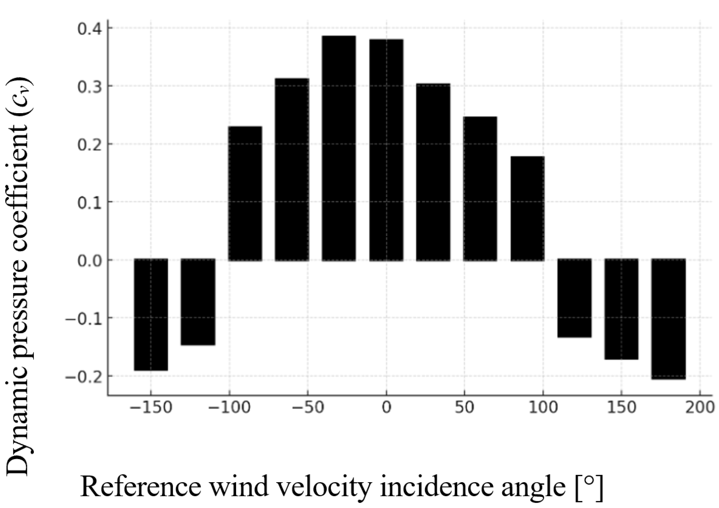
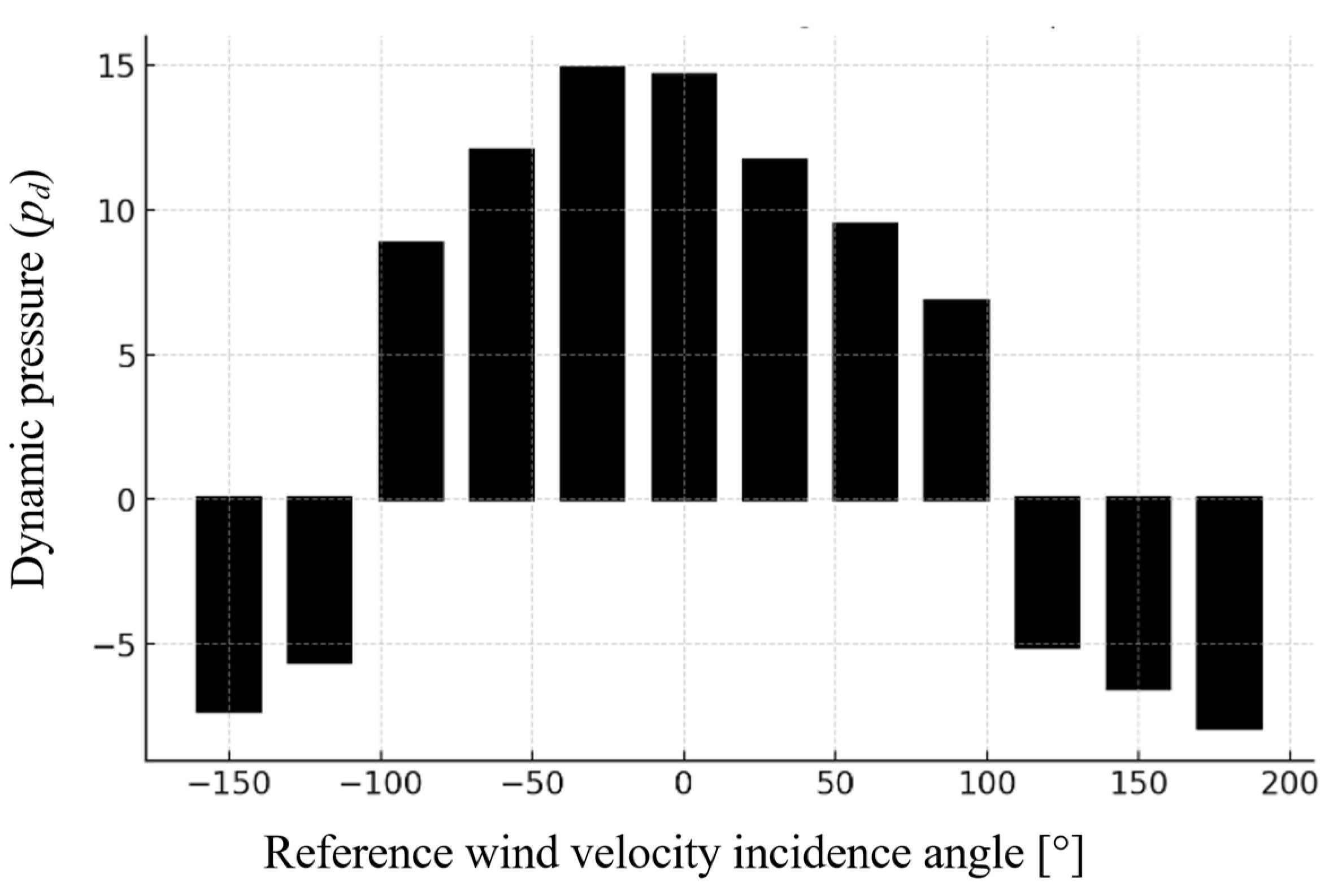
4.3. Results: Gable Roof (Model M1)

The average values of the dynamic pressure coefficient and the corresponding dynamic pressure (Table 2) represent essential parameters in evaluating the distribution of wind-induced forces on the roof surface. These values are determined based on data collected from pressure taps mounted on the roof surface, allowing for a detailed analysis of both local and global variations in wind-induced pressure. The interpretation of dynamic pressure coefficients provides an accurate understanding of how air currents interact with the structure, highlighting areas of high or low pressure—fundamental aspects for optimizing the aerodynamic performance of the roof and ensuring the stability of the photovoltaic system installed on it.
During the wind action testing on the gable roof with photovoltaic panels, relevant data were obtained for various wind incidence angles relative to the horizontal plane. The reference wind velocity used in these experiments was 7.95 m/s, and for each incidence angle, the average values of the dynamic pressure coefficient (Figure 7) and dynamic pressure (Figure 8) were determined. These results are essential for evaluating the structural behavior of the roof under wind influence and identifying potential risk areas.
The aerodynamic response of the gable roof (Model M1) showed significant variations in dynamic pressure coefficients depending on the wind incidence angle. The highest positive values occurred at 0° and –30°, with dynamic pressure coefficients of 0.378 and 0.384, respectively, corresponding to dynamic pressures of 14.63 Pa and 14.86 Pa. These indicate strong frontal compression forces acting directly on the photovoltaic panels.
As the wind angle shifted from frontal to oblique and reverse directions, a progressive decrease in both dynamic pressure and pressure coefficients was observed. At 60° and 90°, the pressure values dropped to 9.48 Pa and 6.85 Pa, respectively. Beyond 120°, the pressure coefficients became negative, indicating suction effects, with the most significant uplift observed at 150° (–0.189) and 180° (–0.204), equating to –7.32 Pa and –7.89 Pa.
This pattern demonstrates a clear aerodynamic transition from compression to uplift, associated with flow separation and vortex formation at higher wind angles. These suction forces are critical, as they generate upward loads that may compromise the structural integrity of the PV mounting system, particularly near panel edges and rear fixings. This observation aligns with [10], who reported elevated suction forces behind PV panels at oblique wind angles on gabled roofs.
The variation in aerodynamic behavior across the incidence angles highlights the sensitivity of gable roofs to wind direction, especially in the context of elevated PV installations. Wind exposure from the rear can generate significant uplift forces, which must be carefully considered during the design and anchorage of PV systems.
In summary, the gable roof configuration exhibited the highest-pressure differentials among the three models tested, confirming its vulnerability to wind-induced uplift. Reinforcement of panel anchoring at rear and edge zones is recommended to enhance structural resilience.

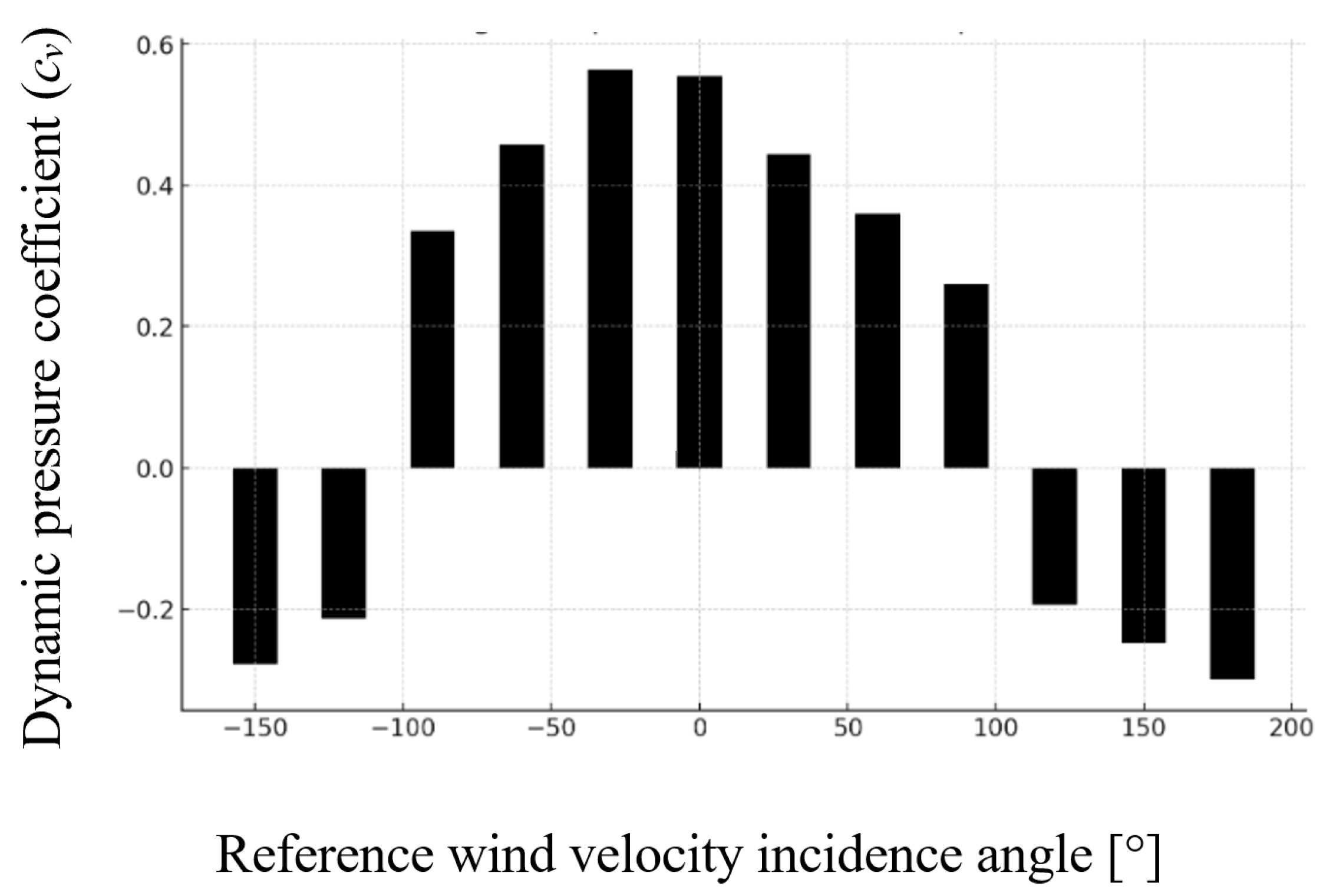
4.4. Results: Hip Roof (Model M2)

The values determined for the dynamic pressure coefficient and dynamic pressure, presented in Table 3, represent essential factors in the analysis of the distribution of aerodynamic forces generated by the wind on the roof. These data are obtained from measurements taken at the pressure taps, optimally placed on its surface, allowing for a detailed assessment of the local and global variations of the pressure exerted by the airflow. Investigating these parameters provides a clear perspective on the areas subjected to significant aerodynamic influences, playing an important role in optimizing the structural configuration and ensuring the stability of the photovoltaic system installed on the roof.
The interpretation of the data in Table 2 provides a detailed perspective on how the wind’s angle of incidence influences the distribution of dynamic pressure on the surface of the roof equipped with photovoltaic panels. The values of the dynamic pressure coefficient (Figure 9) and dynamic pressure (Figure 10) vary significantly depending on the wind direction, indicating both compression and suction zones, phenomena with major implications for the stability of the structure.
The hip roof (Model M2) demonstrated a more uniform aerodynamic response compared to the gable roof. The maximum dynamic pressure coefficient was observed at −30° (cv = 0.564) and 0° (cv = 0.555), corresponding to dynamic pressures of 21.83 Pa and 21.54 Pa, respectively. These indicate strong frontal wind loading on the PV panels mounted on the upper portion of the roof.
As the wind incidence angle increased, the aerodynamic response gradually diminished. At 60° and 90°, the dynamic pressure coefficients decreased to 0.360 and 0.260, indicating a reduced compression effect. Like model M1, suction forces began to appear beyond 120°, with cv values becoming negative. At 150° and 180°, significant suction was recorded (−0.278 and −0.300), with dynamic pressures of −10.75 Pa and −11.61 Pa, respectively.
The more gradual decline in pressure and the smoother transition from compression to suction suggest improved aerodynamic stability. This behavior can be attributed to the hip roof’s sloped geometry on all sides, which facilitates flow deflection and reduces vortex intensity. These findings are consistent with the results of Kopp and Morrison [5], who emphasized the stabilizing effect of hipped roof forms under turbulent wind conditions.
While the hip roof still exhibits areas of suction at higher wind angles, the magnitude of these uplift forces is lower than in the gable configuration. This implies a reduced risk of panel detachment, although anchorage design should still consider rear and lateral suction zones.
Overall, the hip roof configuration showed a balanced aerodynamic profile with lower peak suctions, confirming its relative resilience to wind-induced loading on rooftop PV systems.

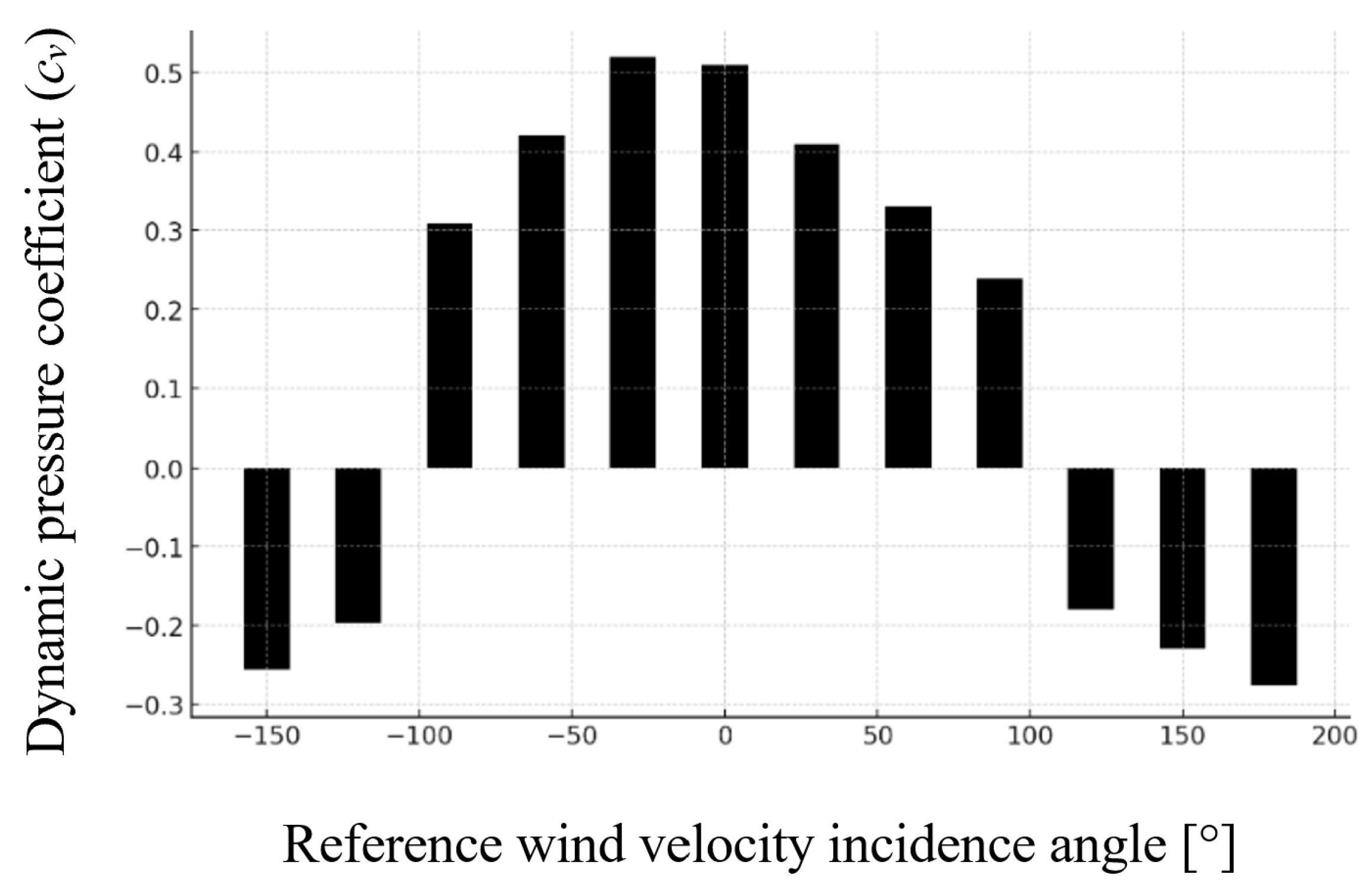
4.5. Results: Multi-Section Roof (Model M3)

The values of the dynamic pressure coefficient and dynamic pressure, presented in Table 4, represent fundamental information for understanding how wind influences the distribution of aerodynamic forces on the roof. These data are extracted from measurements made using pressure taps placed across the entire roof surface, allowing for a detailed evaluation of pressure fluctuations across different areas. The analysis of these parameters helps identify regions subjected to significant aerodynamic loads, which is essential for improving the structural design and ensuring the stability of the photovoltaic system mounted on the roof.
Following the analysis of the results, a significant distribution of the dynamic pressure coefficient (Figure 11) and dynamic pressure (Figure 12) can be observed depending on the wind incidence angle, with maximum and minimum values indicating the variability of the aerodynamic forces applied to the roof.
The multi-section roof (Model M3) displayed a complex aerodynamic behavior, influenced by the variation in roof slopes and junctions between segments. The highest dynamic pressure coefficient was recorded at –30° (cv = 0.626), corresponding to a dynamic pressure of 24.23 Pa, followed closely by 0° (cv = 0.587, pd = 22.72 Pa). These values indicate strong frontal wind loading, especially in zones where PV panels are aligned with roof ridges.
Between 30° and 90°, dynamic pressure coefficients decreased significantly, reaching a minimum of 0.197 at 90°, equivalent to a dynamic pressure of 7.63 Pa. As with the previous models, suction effects emerged beyond 120°, with negative pressure coefficients recorded at 150° and 180° (cv = –0.257 and –0.284, pd = –9.94 Pa and –10.98 Pa, respectively).
Due to its complex geometry, the multi-section roof produced asymmetric flow patterns and non-uniform pressure distributions. This was particularly evident at oblique wind angles (60–120°), where pressure zones shifted unevenly across the roof surface, affecting PV panels mounted on different slopes in distinct ways. These effects mirror those reported in experimental studies on irregular roof shapes, where multiple flow separations and reattachments occur simultaneously [7,21].
The variability in wind-induced pressures across different sections of the roof highlights the challenge of designing uniform anchoring systems for PV modules. Specific zones may experience significantly higher uplift or compression depending on panel orientation relative to wind direction.
In conclusion, the multi-section roof exhibited the most spatially complex pressure behavior, with localized zones of high suction and compression. Customized PV mounting strategies are necessary for such geometries, especially in areas near slope transitions and ridgelines.

5. Conclusions

This study experimentally examined the aerodynamic behavior of photovoltaic (PV) panel systems installed on three different roof configurations—gable, hip, and multi-section—by conducting wind tunnel tests on 1:100 scale models exposed to varying wind incidence angles. The results revealed significant differences in pressure distribution based on roof geometry and wind direction, with gable roofs showing high frontal pressure peaks, hip roofs demonstrating more uniform loading, and multi-segment roofs presenting complex aerodynamic patterns with alternating suction and compression zones.
The presence of negative pressure coefficients at high incidence angles underscores the critical need to account for uplift forces when designing and installing rooftop PV systems. These insights contribute valuable experimental evidence that supports safer and more efficient structural integration of solar technologies, particularly in wind-exposed regions.
Practically, the results suggest that mounting systems for PV panels on gable and multi-pitched roofs should be reinforced especially at edges and corners, where uplift forces are highest. Designers should consider the dominant wind directions in their regions and integrate safety margins for both suction and compression effects when dimensioning supports.
While the results are consistent and statistically reliable, several limitations should be acknowledged. The wind tunnel setup cannot fully replicate real atmospheric turbulence, especially large-scale eddies and gusts. Moreover, the simplifications of model geometry and fixed panel angles may limit the generalizability to irregular installations. Future work should include CFD simulations and full-scale field testing to validate and refine these findings under natural wind conditions.
Beyond the immediate design implications, the findings of this study lay the groundwork for further investigations aimed at enhancing predictive accuracy and structural resilience. Future research should build on this dataset to develop validated numerical simulations, such as CFD models, capable of extrapolating the observed aerodynamic phenomena to full-scale conditions. Additionally, extended studies could explore the long-term behavior of PV mounting systems under fluctuating wind loads and help inform updates to design standards for complex roof geometries.
In this context, the current work serves not only as a contribution to experimental wind engineering but also as a reference point for ongoing research efforts focused on integrating renewable energy systems safely and sustainably into the built environment.
Given the increasing emphasis on sustainable development in civil engineering, this study offers practical guidance for enhancing the reliability of solar energy systems in diverse architectural contexts. By improving the understanding of wind effects on PV-equipped roofs, the research supports informed decisions in both design and policy, contributing to the broader objectives of environmental responsibility, energy efficiency, and resilience in the built environment.

Author Contributions

Conceptualization, R.-A.P., N.Ţ. and S.-V.H.; methodology, R.-A.P., N.Ţ. and D.U.; software, R.-A.P. and M.A.; validation, S.-V.H., D.U. and I.H.; formal analysis, R.-A.P., C.O., M.A. and I.H.; investigation, R.-A.P., C.O. and A.-F.M.; resources, N.Ţ.; data curation, S.-V.H., C.O., M.A. and I.H.; writing—original draft preparation, R.-A.P., N.Ţ. and S.-V.H.; writing—review and editing, R.-A.P., N.Ţ., S.-V.H. and I.H.; visualization, R.-A.P., D.U. and A.-F.M.; supervision, N.Ţ.; project administration, R.-A.P. and N.Ţ.; funding acquisition, N.Ţ. All authors have read and agreed to the published version of the manuscript.

Funding

This research received no external funding.

Institutional Review Board Statement

Not applicable.

Informed Consent Statement

Not applicable.

Data Availability Statement

The data presented in this study are available on request from the corresponding author.

Conflicts of Interest

The authors declare no conflicts of interest.

References

  1. Polcovnicu, R.A.; Ţăranu, N.; Ungureanu, D.; Sbîrlea, C.; Cozmanciuc, R. Building Integrated Photovoltaics Systems: State-of-the-Art Review. Bull. Inst. Politeh. Iași. Archit. Sect. 2021, 67, 71. [Google Scholar] [CrossRef]
  2. Polcovnicu, R.A.; Ţăranu, N.; Ungureanu, D.; Zghibarcea, Ș.V.; Hudișteanu, V.S. Modern Manufacturing Technology for Modular Photovoltaic Panels: State-of-the-Art and Future Trends. In IOP Conference Series: Materials Science and Engineering; IOP Publishing: Bristol, UK, 2020; p. 1182. [Google Scholar]
  3. Eslami Majd, A.; Adebayo, D.S.; Tchuenbou-Magaia, F.; Willetts, J.; Nwosu, D.; Matthews, Z.; Ekere, N.N. Wind Flow and Its Interaction with a Mobile Solar PV System Mounted on a Trailer. Sustainability 2024, 16, 2038. [Google Scholar] [CrossRef]
  4. Jackson, A.; Donaldson, G.; Gómez-Amo, J. Impact of Extreme Weather Conditions on the Performance of Utility-Scale PV Systems. Sustainability 2023, 15, 731. [Google Scholar]
  5. Tu, Z.; Zheng, G.; Yao, J.; Shen, G.; Lou, W. Computational Investigation of Wind Loads on Tilted Roof-Mounted Solar Array. Sustainability 2022, 14, 15653. [Google Scholar] [CrossRef]
  6. Kopp, G.A.; Morrison, M.J. Wind Effects on Rooftop-Mounted Solar Photovoltaic Systems. J. Struct. Eng. 2018, 144, 04018001. [Google Scholar]
  7. Khadimallah, M.A.; Abdelbaky, M.; Bouafia, Y. Numerical Modeling of Wind Loads on Solar PV Arrays in Built Environments. J. Wind Eng. Ind. Aerodyn. 2024, 200, 104985. [Google Scholar]
  8. Ke, Y.; Shen, G.; Yang, X.; Xie, J. Effects of Surface-Attached Vertical Ribs on Wind Loads and Wind-Induced Responses of High-Rise Buildings. Sustainability 2022, 14, 11394. [Google Scholar] [CrossRef]
  9. Aly, A.M.; Rone, E. Wind Loads on a Low-Rise Gable Roof with and without Solar Panels and Comparison to Design Standards. Sustain. Resil. Infrastruct. 2024, 9, 589–609. [Google Scholar] [CrossRef]
  10. Hudisteanu, S.V.; Popovici, C.G. Experimental investigation of the wind direction influence on the cooling of photovoltaic panels integrated in double skin facades. E3S Web Conf. 2019, 111, 03045. [Google Scholar] [CrossRef]
  11. Wang, L.; Shi, F.; Wang, Z.; Liang, S. Blockage Effects in Wind Tunnel Tests for Tall Buildings with Surrounding Buildings. Appl. Sci. 2022, 12, 7087. [Google Scholar] [CrossRef]
  12. Peng, H.Y.; Liang, H.; Dai, S.F.; Liu, H.J. Wind load analysis for rooftop solar photovoltaic panels in the presence of building interference: A wind tunnel study. J. Build. Eng. 2025, 100, 111702. [Google Scholar] [CrossRef]
  13. Hudișteanu, S.V.; Ţurcanu, F.E.; Cherecheș, N.-C.; Popovici, C.-G.; Verdeș, M.; Ancaș, D.-A.; Hudișteanu, I. Effect of Wind Direction and Velocity on PV Panels Cooling with Perforated Heat Sinks. Appl. Sci. 2022, 12, 9665. [Google Scholar] [CrossRef]
  14. EN 1991-1-4:2005+A1:2010; Eurocode 1: Actions on Structures—Part 1–4: General Actions—Wind Actions. CEN: Brussels, Belgium, 2010.
  15. Zhang, J.; Lou, Y. Study of Wind Load Influencing Factors of Flexibly Supported Photovoltaic Panels. Buildings 2024, 14, 1677. [Google Scholar] [CrossRef]
  16. Geurts, C.; van Bentum, C. Wind Loading on Buildings: Eurocode and Experimental Approach; CISM International Centre for Mechanical Sciences; Springer: Vienna, Austria, 2007; Volume 493. [Google Scholar] [CrossRef]
  17. Yao, J.; Tu, Z.; Wang, D.; Shen, G.; Lou, W. Experimental Investigation of Wind Loads on Roof-Mounted Solar Arrays. Sustainability 2022, 14, 8477. [Google Scholar] [CrossRef]
  18. Wang, W.; Zhu, Y.; Shu, Z.; Li, Y. A Review on Aerodynamic Characteristics and Wind-Induced Response of Flexible Support Photovoltaic System. Atmosphere 2023, 14, 731. [Google Scholar] [CrossRef]
  19. Nezamisavojbolaghi, M.; Davodian, E.; Bouich, A.; Tlemçani, M.; Mesbahi, O.; Janeiro, F.M. The Impact of Dust Deposition on PV Panels’ Efficiency and Mitigation Solutions: Review Article. Energies 2023, 16, 8022. [Google Scholar] [CrossRef]
  20. Wang, J.; Liu, M.; Yang, Q.; Hui, Y.; Nie, S. Extreme Wind Loading on Flat-Roof-Mounted Solar Arrays with Consideration of Wind Directionality. Buildings 2024, 14, 221. [Google Scholar] [CrossRef]
  21. Hu, J.; Wang, X.; Yang, H.; Huang, B. Experimental Study on Rooftop Flow Field of Building Based on the Operation of Vertical-Axis Wind Turbines. J. Renew. Sustain. Energy 2024, 16, 053301. [Google Scholar] [CrossRef]
  22. Shen, G.; Yu, S.; Lou, W. Experimental Investigation of the Parapet Effect on the Wind Load of Roof-Mounted Solar Arrays. Sustainability 2023, 15, 5052. [Google Scholar] [CrossRef]
  23. Kopp, G.A.; Banks, D. Use of Wind Tunnel Measurements in Wind Load Design of Solar Panels. J. Wind Eng. Ind. Aerodyn. 2013, 123, 232–240. [Google Scholar]
  24. Li, S.; Xiao, F.; Li, S.; Hui, Y.; Yang, Q.; Li, B.; Chen, Y.; Zhou, S.; Liu, M. Wind Loads on Solar Panels Mounted on Facade of High-Rise Residential Building. Int. J. Struct. Stab. Dyn. 2024, 24, 2240019. [Google Scholar] [CrossRef]
  25. ASME. Numerical Simulation of Wind Load on Roof-Mounted Solar Panels. In Proceedings of the ASME International Conference, Boston, MA, USA, 30 June–2 July 2014. [Google Scholar]
  26. ICRAES-2020. Wind Pressure Distribution on PV Panels Mounted on Saw-Type Roofs. In Proceedings of the International Conference on Recent Advances in Engineering & Science, New York, NY, USA, 17 November 2020. [Google Scholar]
  27. ASCE/SEI 7-22; Minimum Design Loads and Associated Criteria for Buildings and Other Structures. American Society of Civil Engineers: Reston, VA, USA, 2022.
  28. Bendat, J.S.; Piersol, A.G. Random Data: Analysis and Measurement Procedures, 4th ed.; Wiley: Hoboken, NJ, USA, 2010. [Google Scholar]
  29. Spanelis, A.; Georgiou, D. Assessment of Aerodynamic Wake Effects on PV-Mounted Rooftops. Resources 2023, 12, 90. [Google Scholar]
Figure 1. The wind tunnel at the Building Aerodynamics Laboratory, “Gheorghe Asachi” Technical University of Iași.
Sustainability 17 04739 g001
Figure 2. Instruments used for measurements in the wind tunnel: (a) pressure sensor plate and connecting tubes; (b) Pitot tube; (c) digital anemometer.
Sustainability 17 04739 g002
Figure 3. Recording circuit: data acquisition board—pressure transducers—model.
Sustainability 17 04739 g003
Figure 4. House with a gable roof model at scale 1:100 (M1).
Sustainability 17 04739 g004
Figure 5. House with a hip roof model at the scale of 1:100 (M2).
Sustainability 17 04739 g005
Figure 6. Institutional building with a multi-section roof model at the scale 1 to 100 (M3).
Sustainability 17 04739 g006
Figure 7. Graph showing the variation of dynamic pressure coefficient for the gable roof model (M1) as a function of wind incidence angle, highlighting zones of compression and suction.
Sustainability 17 04739 g007
Figure 8. Corresponding dynamic pressure values for the gable roof model (M1), indicating higher pressure loads at 0° and −30° angles.
Sustainability 17 04739 g008
Figure 9. Dynamic pressure coefficient distribution for the hip roof model (M2), revealing more uniform aerodynamic behavior than the gable roof.
Sustainability 17 04739 g009
Figure 10. Dynamic pressure values across wind incidence angles for the hip roof model (M2), with peak values at frontal wind directions and suction observed at rear angles.
Sustainability 17 04739 g010
Figure 11. Coefficient of dynamic pressure variation for the multi-section roof model (M3), showing irregular behavior due to complex geometry.
Sustainability 17 04739 g011
Figure 12. Recorded dynamic pressure values for the multi-section roof model (M3), reflecting both peak compressive and uplift forces.
Sustainability 17 04739 g012
Table 1. Summary of the main experimental conditions and testing parameters applied to the three scaled roof models in the wind tunnel setup.
ParameterDescription
Test facilityWind tunnel with turbulent boundary layer, Technical University of Iași
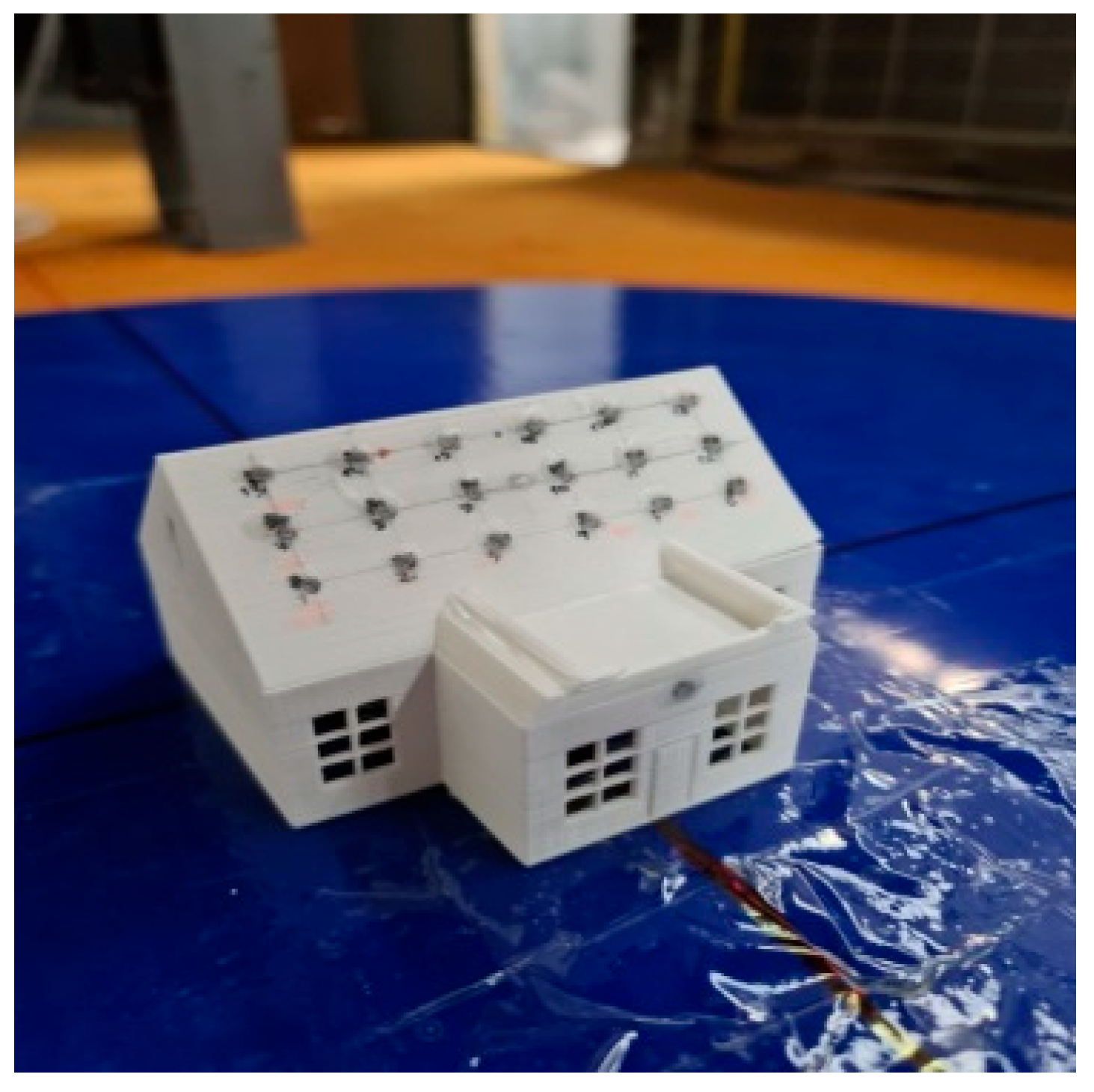
Scale of physical models1:100
Roof types testedM1—Gable, M2—Hip, M3—Multi-section
Number of sensors per model18 pressure sensors + 1 reference sensor
Wind incidence angles0°, ±30°, ±60°, ±90°, ±120°, ±150°, 180° (12 angles total)
Reference wind speed7.95 m/s
Duration per test30 s
Number of samples per test30,000
Total number of tests36 (12 per model)
Data acquisition frequency1000 Hz
Software usedLABVIEW and custom processing scripts
Table 2. Average values of the dynamic pressure coefficient and corresponding dynamic pressure for the gable roof model (M1) at 7.95 m/s reference wind speed, across 12 wind incidence angles.
Reference Wind Speed (vref) [m/s]Angle of Incidence of Reference Wind Speed [°]Average Dynamic Pressure Coefficient (cv)Dynamic Pressure (pd) [Pa]
7.950.37814.63
30°0.30211.69
60°0.2459.48
90°0.1776.85
120°−0.132−5.11
150°−0.169−6.54
180°−0.204−7.89
−30°0.38414.86
−60°0.31112.04
−90°0.2288.82
−120°−0.145−5.61
−150°−0.189−7.32
Table 3. Summary of the dynamic pressure coefficients and pressures measured for the hip roof model (M2) under controlled wind tunnel conditions, showing variation by incidence angle.
Reference Wind Speed (vref) [m/s]Angle of Incidence of Reference Wind Speed [°]Average Dynamic Pressure Coefficient (cv)Dynamic Pressure (pd) [Pa]
7.950.55521,536
30°0.44417,190
60°0.36013,926
90°0.26010,055
120°−0.194−7511
150°−0.248−9617
180°−0.300−11,611
−30°0.56421,827
−60°0.45717,095
−90°0.33512,964
−120°−0.213−8252
−150°−0.278−10,752
Table 4. Experimental results for the multi-section institutional roof model (M3), highlighting both positive and negative pressure effects across varying wind directions.
Reference Wind Speed (vref) [m/s]Angle of Incidence of Reference Wind Speed [°]Average Dynamic Pressure Coefficient (cv)Dynamic Pressure (pd) [Pa]
7.950.51019,809
30°0.40915,830
60°0.33112,822
90°0.2399257
120°−0.179−6910
150°−0.229−8859
180°−0.276−10,682
−30°0.52020,094
−60°0.42115,730
−90°0.30911,933
−120°−0.196−7593
−150°−0.256−9892
Disclaimer/Publisher’s Note: The statements, opinions and data contained in all publications are solely those of the individual author(s) and contributor(s) and not of MDPI and/or the editor(s). MDPI and/or the editor(s) disclaim responsibility for any injury to people or property resulting from any ideas, methods, instructions or products referred to in the content.

