The Synergistic Effect of Foreign Direct Investment and Renewable Energy Consumption on Environmental Pollution Mitigation: Evidence from Developing Countries

Abstract

Global efforts to reduce climate change have increased, necessitating more comprehensive research. However, empirical evidence of the implication of synergizing foreign direct investment (FDI) and renewable energy consumption (REC) to reduce environmental pollution, specifically with nitrous oxide (N₂O) and methane (CH₄) emissions, is missing in the literature. This research investigates the impact of FDI, REC and their synergy in facilitating technological leapfrogging, analyzing their linear, non-linear and indirect effects on environmental pollution (CO₂, N₂O and CH₄ emissions). The analysis focuses on 81 developing countries, analyzing them at both the general level and by income groups—low-income countries (LICs), middle-income countries (MICs) and high-income countries (HICs), with government effectiveness and economic growth serving as mediating variables. Using Canonical Correlation Regression (CCR), Fully Modified Ordinary Least Squares (FMOLS) and clustered Pooled Least Square (PLS) techniques, the analysis covers data from 2003 to 2023. The results indicate that at the general level, FDI and REC increase N₂O and CH₄ emissions individually. However, their integration mitigates N₂O and CH₄ emissions. Additionally, the relationships remain consistent even when government effectiveness and economic growth are considered mediators. However, economic growth is more pronounced than government effectiveness in reducing environmental pollution. The non-linear analysis also reveals that FDI and REC have a significant U-shaped effect on CO₂ emissions. However, their synergy demonstrates an inverted U-shaped nexus with CO₂ emissions. At the income group levels, the interplay of FDI and REC reduces N₂O and CH₄ emissions in MICs; however, in LICs and HICs, it increases N₂O and CH₄ emissions.

1. Introduction

In environmental sustainability, foreign direct investment (FDI) and renewable energy consumption (REC) have materialized as essential factors contributing to climate change, specifically in developing nations. FDI is considered the quiddity of more developing nations over the past decades [1]. According to Marques and Caetano [2], FDI is one of the lifebloods of globalization. However, its environmental impact has also emerged as an increasing concern. With the maximum level of effort to attract more FDIs, many environmentally unfriendly industries from developed nations move to developing nations due to the stern policies and high expenses of pollution reduction in the developed nations. This is considered in the environmental literature as the “pollution haven hypothesis” [3]. This hypothesis validates the claim that most developed countries have reduced emissions by transferring contaminating projects to developing nations [4].

Developing countries are key players in the international combat against climate change, yet they encounter tremendous challenges, including unavailable renewable energy technologies and financial constraints. FDI can address these challenges by facilitating the funding of renewable energy projects. It can channel financial and technological resources into the renewable energy industry to accelerate the transformation to cleaner energy systems. Moreover, industrialization in developing nations is traditionally associated with increased environmental pollution due to the reliance on energy-intensive and fossil-fuel-based technologies. However, the advent of FDI and the growing global emphasis on renewable energy can offer a unique opportunity for these countries to forgo polluting stages of development through a process known as technological leapfrogging. Technological leapfrogging allows developing nations to adopt advanced and clean technologies without first undergoing environmental degradation.

As literature widely underpins the idea that FDI and REC can affect emissions, the specific impact on the major greenhouse gases (GHGs) is rarely investigated, especially in the context of developing nations. Carbon dioxide (CO₂), nitrous oxide (N₂O) and methane (CH₄) emissions pose different environmental challenges, each contributing separately to climate change. CO₂ emissions are a significant source of anthropogenic climate change, primarily related to industrial duties, energy production and deforestation [5]. N₂O, as a dominant GHG, is discharged through agricultural activities, industrial tasks and the application of nitrogen-based fertilizers [6]. Over the past centuries, the rising level of N₂O emissions has promoted stratospheric ozone reduction. This is determined with an updated level of a 2% increment per decade [7]. CH₄ emissions are another primary source of global warming [8]. It also has natural occurrences as well as the outcomes from human activities. According to the report of the United Nations Environment Program [9], CH₄ is a harmful GHG, responsible for 1 million premature deaths annually. Over the past decades, methane has been 80 times more productive in trapping atmospheric heat than CO₂ emissions. However, most air pollution management is centered on mitigating CO₂ emissions; there is less focus on other GHGs [10].

This paper explores how FDI and REC can be synergized, enabling technological leapfrogging to contribute to environmental pollution mitigation in developing countries. Therefore, the study analyzes the direct and non-linear effects of FDI, REC and their integration on GHGs. It also focuses on the mediating effects of government effectiveness and economic growth on environmental pollution. The study contradicts existing literature, as research on the effects of FDI and REC on GHGs often centers on CO₂ emissions, neglecting their potential differential effect on other GHGs [11]. Additionally, studies by scholars such as Liu et al. [12], Paul et al. [13] and Islam et al. [14] investigated only the direct and individual impact of FDI and REC on CO₂ emissions. However, this paper seeks to comprehensively examine the linear and non-linear influence of FDI, REC and their integration on multiple GHGs simultaneously. Moreover, it ascertains how government effectiveness and economic growth mediate the role of FDI, REC and their synergy on environmental pollution mitigation. This surpasses traditional linear assumptions, adopts a synergistic approach to explore their interactive effects and complementarity and provides a more pronounced analysis of how these indicators interact across varied adoption and policy integration levels. Furthermore, the study categorizes the developing countries into income groups: low-income countries (LICs), middle-income countries (MICs) and high-income countries (HICs). This approach ensures that the findings are practical, context-sensitive and aligned with global sustainability goals, promoting the academic rigor and real-world applicability of the research. Section 1 introduces and provides the background for this study. The remainder of the paper is organized as follows: Section 2—Literature Review; Section 3—Methodology; Section 4—Results and Discussion; Section 5—Conclusion and Recommendation.

2. Theoretical, Empirical Literature and Study Hypotheses

2.1. FDI and Environmental Pollution

Governments are striving to reduce GHGs while ensuring a developed economy significantly. According to Sheng et al. [15], researchers investigating the nexus between FDI inflows and GHGs, particularly CO₂ emissions, often reference the “pollution haven” and “pollution halo” theories. The pollution haven theory asserts that international industries, specifically those involved in heavily polluted projects, identify nations with weak environmental policies for their investments. Unlike the strict ecological policies implemented in developed nations, these international industries transfer their manufacturing processes to the least developed nations due to the low cost and ease of complying with slack environmental standards [16]. Notwithstanding, if developing nations can leapfrog traditional pollution-intensive industries and instead attract clean technologies, this would mitigate the risk of becoming pollution havens. Scholars such as Abbasi et al. [17], Ozcelik et al. [18], Ozkan et al. [19] and Chiriluș and Costea [20] have validated this hypothesis through their findings. Ozcelik et al. [18] examined the role of FDI in CO₂ emissions for BRICMT (Brazil, Russia, India, China, Mexico, Turkey) nations, validating the existence of the pollution haven theory. Similarly, Chiriluș and Costea [20] explored the connection between FDI and sustainability, further validating the pollution haven theory.

However, the “pollution halo” theory argues that FDI inflows provide modernized manufacturing tools, professional leadership experience and structured renewable energy technologies. These can enhance efficient and effective production, expand technological and leadership creativity and innovation and mitigate GHGs in the host countries [15]. FDI, specifically in clean technologies, can allow developing nations to leap over traditional high-emission development stages and improve their ecological and economic performance. The pollution halo effect, therefore, can be a key driver of technological leapfrogging in renewable energy. Countless researchers have explored this theory after its introduction. Liu et al. [21] analyzed the role of Chinese FDI in ecological sustainability for Belt and Road nations and supported the halo hypothesis. Moreover, Liu and Guo [22] chose the spatial econometric model to ascertain the correlation between FDI and environmental quality in Chinese cities and confirmed the halo hypothesis.

Empirical studies of FDI on environmental pollution mitigation offer essential insights into the complex dynamics shaping the region’s ecological landscape. However, their findings show a varied outcome; some studies report a positive and U-shaped relationship, while others provide a negative, inverted U-shape and insignificant findings. For instance, Abbasi et al. [17] concluded that FDI positively influenced CO₂ emissions in Asian countries using the autoregressive distributed lag (ARDL) model. Similarly, a year of data covering 1990–2018 for 200 countries was utilized by Paul et al. [13] to ascertain the implication of FDI on CO₂ and N₂O emissions. The study indicated that FDI proliferates these GHGs. An investigation into the nexus between FDI and CO₂ emissions was conducted by Apergis et al. [23] for the BRICS (Brazil, Russia, India, China and South Africa) nations. The findings revealed that inflows from Denmark and the United Kingdom intensify CO₂ emissions in BRICS nations. However, the results from Islam et al. [14] and Bello et al. [24] showed a negative connection between FDI and CO₂ emissions in Bangladesh and the Association of Southeast Asian Nations (ASEAN) using ARDL and the vector error correction model (VECM) accordingly. Moreover, using spatial and panel-corrected standard error (PCSE) models, Sheng et al. [15] and Olatunde et al. [25] revealed that FDI insignificantly influences ecological pollution in sub-Saharan Africa (SSA) and 30 Chinese provinces, respectively. Abdul-Mumuni et al. [26] concluded that an inverted U-shaped connection exists between FDI and CO₂ emissions for 41 SSA nations by using the non-linear autoregressive-distributed lag (NARDL) technique. In contrast, Xu et al. [27] focused on provinces in Chinese to investigate the non-linear effect of FDI on natural gases and concluded a U-shaped interrelationship exists.

2.2. REC and Environmental Pollution

Promoting REC is critical for curbing GHGs, enhancing air quality and ensuring long-lasting energy security. The energy transition theory emphasizes the change from one prevalent energy source to another, explicitly transforming from less-effective to more-productive energy options [28]. Technological leapfrogging is critical to energy transitions, especially in developing nations. Thus, instead of focusing on the traditional stages of energy system development, such as heavy reliance on coal and oil, developing countries can leap directly to renewable energy sources, skipping over the “dirty” stages of industrialization. The global community has undergone energy transformations from wooden material to coal and oil [29]. The current phase, which this paper focuses on, involves transitioning from carbon-based energy—primarily coal and oil—to lesser-carbon energy sources such as natural gas, wind, solar and hydropower. After the world oil crisis in the 1970s, countless nations have executed energy transformation strategies to resolve different energy challenges [30]. Achieving a zero-carbon future to meet global carbon neutrality goals presents a significant problem. In this context, the energy industry is a key player in addressing this challenge [31]. To meet the vision for net-zero emissions and restrict global warming to 1.5 °C by 2050, it is essential to develop a long-lasting, effective and robust energy system [32].

Donkor et al.’s [33] findings from 41 African nations on policy integration and renewable energy deployment suggested that REC decreases CO₂ emissions but increases N₂O emissions. Azam et al. [34] and Liu et al. [12] examined the contribution of REC to ecological sustainability for the ten countries with the highest CO₂-emitting emissions and 30 provinces in China, respectively. The research indicated that a rise in REC proliferates the intensity of CO₂ emissions. Notwithstanding, the results of Gierałtowska et al. [35] and Zeeshan et al. [36], who also ascertained the environmental impact of REC on ecological pollution for 136 countries and ASEAN nations, showed that REC significantly mitigates CO₂ emissions. Due to the inconsistent findings on the role of FDI and REC on ecological pollution, this paper synergizes these variables and assumes the following hypotheses:

H1. 

Synergizing FDI and REC contributes to technological leapfrogging and validates the pollution halo and energy transition theories, mitigating environmental pollution in developing nations.

H2. 

SynergizingFDI and REC reveals a U-shaped relationship with environmental pollution in developing nations.

2.3. Government Effectiveness and Environmental Pollution

Scholars have emphasized that constructive governance is essential for achieving ecological sustainability. Asongu and Odhiambo [37] analyzed the influence of governance on ecological performance in SSA. Their findings highlight that government effectiveness shows an insignificant connection with CO₂ emissions. Donkor et al. [38] explored the pursuit of a cleaner environment in Africa and found that in resource-rich countries, government effectiveness intensifies CO₂ emissions but curbs N₂O emissions. In contrast, in resource-poor economies, CO₂ emissions reduce with improved governance quality but increase with enhanced government effectiveness. Adekunle [39] examined the contribution of governance in achieving ecological sustainability. The findings demonstrated a negative correlation between government effectiveness and ecological sustainability. Dincă et al. [40] revealed that government effectiveness positively impacts ecological performance. Similarly, Simionescu et al. [41] also discovered how governance indicators intensify pollution levels. These studies highlight the critical role of government effectiveness in contributing to environmental sustainability. Based on these outcomes, this paper hypothesizes the following:

H3. 

Government effectiveness, as a mediating variable for the synergy of FDI and REC, significantly increases developing nations’ environmental pollution.

2.4. Economic Growth and Environmental Pollution

Economic growth and ecological pollution are closely interconnected, with economic development often resulting in increased resource usage and greater pollution levels. Byaro et al. [42] ascertained the mediating role of institutional quality in the connection between economic growth and ecological sustainability. The outcome revealed that GDP unfavorably affects environmental sustainability in Asian nations. Similarly, Donkor et al. [43] analyzed the link between economic growth and ecological quality, concluding that GDP significantly increases CO₂ emissions in northern and southern nations, with a one-way causation from GDP to CO₂ emissions. Moreover, Xue et al. [44] identified a positive correlation between GDP and CO₂ emissions, estimating that a 1% increase in GDP expands CO₂ emissions, assuming other factors remain constant. Furthermore, Yang and Khan [45] concluded that GDP exacerbates CO₂ emissions in the short term. Espoir et al. [46] also examined the dynamic impact of GDP on ecological pollution and discovered that GDP per capita results in increased emissions in the long run. Considering the findings of these studies, this paper hypothesized the following:

H4. 

Economic growth, as a mediating variable for the synergy of FDI and REC, significantly increases environmental pollution in developing nations.

3. Data and Methodology

3.1. Data

This paper analyzes eighty-one (81) developing countries recognized by the UN. It examines these countries at both their general level and income groups—LICs, MICs and HICs. Developing countries have become major destinations for FDI [1], driven by their growing markets, abundant natural resources and lower labor costs. Simultaneously, energy demand in these regions is rising due to economic growth and population expansion. This creates a unique opportunity to study how FDI and renewable energy consumption interact in such dynamic environments. This research relies strongly on secondary data from the World Bank’s World Development Indicator (WDI) and World Governance Indicator (WGI) databases covering 2003 to 2023. As shown in

Table 1. Variable description.

Variable	Description	Unit	Sources
CO2	Carbon dioxide emissions	Metric tons	WDI (2025)
N2O	Nitrous oxide emissions	Metric tons of CO2 equivalent	WDI (2025)
CH4	Methane emissions	Metric tons of CO2 equivalent	WDI (2025)
FDI	Foreign direct investment	Total FDI inflows (USD)	WDI (2025)
REC	Renewable energy consumption	Percentage of total final energy consumption	WDI (2025)
FR	Synergy of FDI and REC	A combination of FDI and REC	WDI (2025)
GOVE	Government effectiveness	Percentile rank	WGI (2025)
GDP	Gross Domestic Product (current)	USD	WDI (2025)
IND	Industrialization	Percentage of GDP	WDI (2025)
TOP	Trade openness	Trade (% of GDP)	WDI (2025)
POP	Total population	Total	WDI (2025)
GOVS	Government spending	Percentage of GDP	WDI (2025)

, CO₂, N₂O and CH₄ emissions are separately used as the dependent variables. FDI, REC and their synergy (FR) are utilized as the core explanatory variables, and government effectiveness (GOVE) and GDP are chosen as mediating variables. Other control variables used are industrialization (IND), trade openness (TOP), total population (POP) and government spending (GOVS).

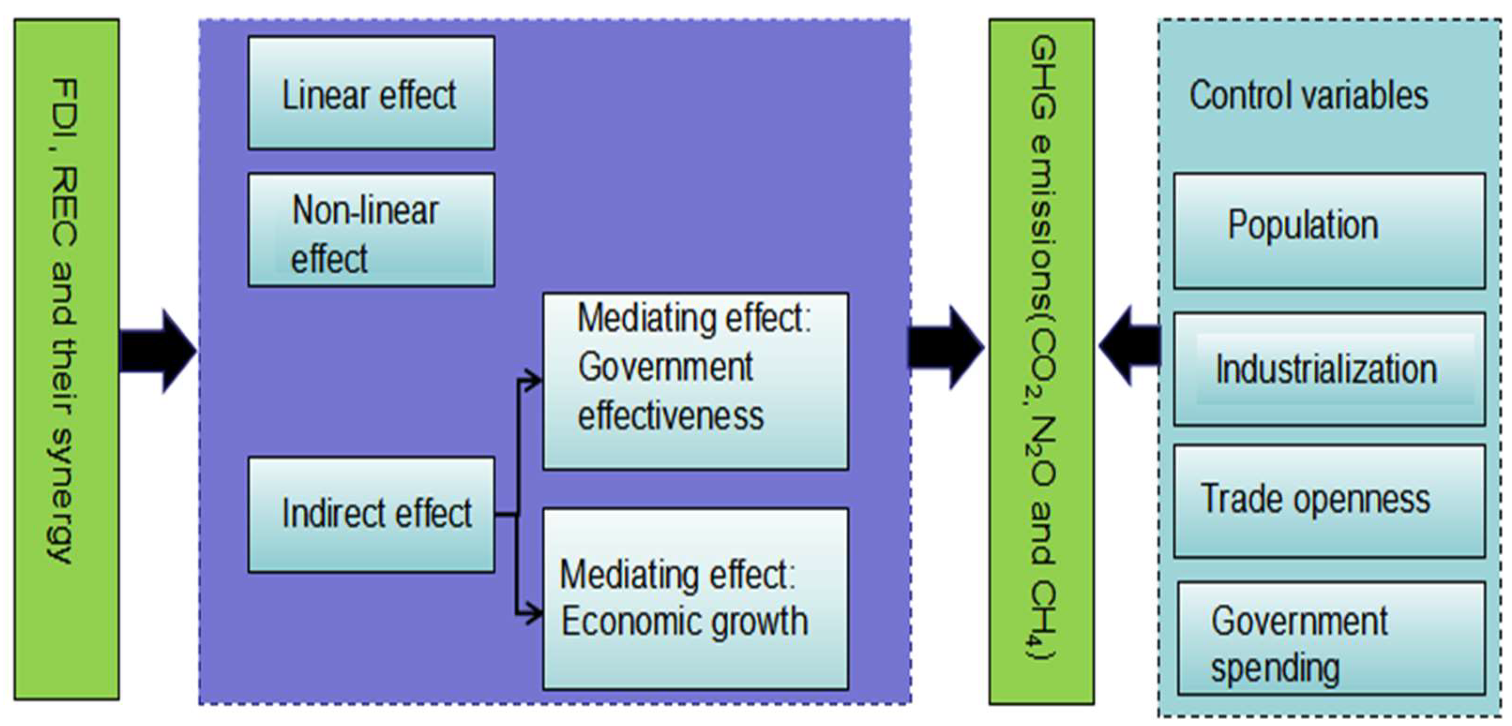
3.2. Research Framework

This research explores the linear, non-linear and indirect roles of FDI, REC and their synergy on GHGs, with government effectiveness and economic growth as mediators (see Figure 1).

3.3. Data Normalization

Due to the larger range of figures with separate variables, the data are normalized to keep a standardized format. This eliminates the enormous variations in the numerical association among the indicators and permits various types of indicators employed to be assessed within a stipulated interval. n is denoted as the number of samples first chosen, and m is the number of employed indicators. The data are normalized using Equations (1) and (2). Equation (1) is applied when the chosen indicators positively impact the dependent indicators, while Equation (2) is used in cases where the relationship is negative. These are shown below:

$$X_{it}=\left(x_{it}-\mathit{min}\left(x_t\right)\right)÷\left(\mathit{max}\left(x_t\right)-\mathit{min}\left(x_t\right)\right), i=1, 2, 3, \dots n; t=1, 2, 3, \dots m$$

(1)

$$X_{it}=\left(\mathit{max}\left(x_t\right)-x_{it} \right)÷\left(\mathit{max}\left(x_t\right)-\mathit{min}\left(x_t\right)\right), i=1, 2, 3, \dots n; t=1, 2, 3, \dots m$$

(2)

where $X_{it}$ and $x_{it}$ indicate the normalized and original figures for a variable, with n representing all the years; $\mathit{max}\left(x_t\right)$ and $\mathit{min}\left(x_t\right)$ signify the maximum and minimum figures for each variable with n in all the years.

3.4. Model Specification

This paper employs panel data analysis models, specifically Canonical Correlation Regression (CCR) and Fully Modified Ordinary Least Squares methods (FMOLS) using STATA 17 software to examine linear, non-linear and indirect analyses. Clustered Pooled Least Square (PLS) is also chosen as an alternative estimation technique to validate the findings of the linear and non-linear analyses. FMOLS effectively addresses issues of asymptotic bias and dependence on nuisance parameters associated with estimating cointegrating vectors in traditional single-equation models. This method has proven capable of resolving various challenges linked to these complexities. It has gained prominence in highlighting its advantageous properties in the context of nonstationary vector autoregressions (VARs) with unknown cointegrating ranks. FMOLS evaluation only modifies the regressand:

$$y_t^{+}=y_t-{\widehat{w}}_{12}{\widehat{\Omega }}_{22}^{-1}{\widehat{u}}_{2t}$$

(3)

where ${\widehat{u}}_{2t}$ is the residual of the cointegration equation estimated by ordinary least square (OLS), and ${\widehat{u}}_{2t}$ is the differenced residuals of regressor equations or those of the differenced regressor equations.

The FMOLS estimators and their covariance are given by

$$\widehat{\theta }=\left[\begin{array}{c}\widehat{B}\\ {\widehat{r}}_1\end{array}\right]=\left[{\sum }_{t=1}^T{z}_t{z}_t^{\prime }\right] \left[{\sum }_{t=1}^T{z}_t{y}_t^{+}-T\left(\begin{array}{c}{\widehat{\lambda }}_{12}^{{+}^{\prime }}\\ 0\end{array}\right)\right]$$

(4)

$$Var \widehat{\left(\theta \right)}={\widehat{w}}_{\mathrm{1,2}}\left[{\sum }_{t=1}^T{z}_t{z}_t^{\prime }\right], {\widehat{w}}_{\mathrm{1,2}}={\widehat{w}}_{11}-{\widehat{w}}_{12}{\widehat{\Omega }}_{22}^{-1}{\widehat{u}}_{21}$$

(5)

where ${\widehat{\lambda }}_{12}^{+}={\widehat{\lambda }}_{12}-{\widehat{w}}_{12}{\widehat{\Omega }}_{22}^{-1}{\widehat{\wedge }}_{22}$ are called bias-correction terms. $z_t=(x_t^{\prime },d_{1t}^{\prime }{)}^{\prime }$. ${\widehat{w}}_{\mathrm{1,2}}$ is the estimate of the long-run covariance of $U_{1t}$ conditional on $U_{2t}$.

Moreover, the CCR method applies to various cointegration models, including deterministic, singular, stochastic and regular cointegrations. It provides asymptotically efficient estimators and ensures that asymptotic chi-square tests are free from nuisance parameters. The FMOLS and CCR estimators are derived by adjusting the independent and dependent variables and applying the OLS technique. In the CCR approach, the regressand and the regressors are modified in the evaluation process.

$$y_t^{+}=y_t-\left\{{\widehat{\Sigma }}^{-1}{\widehat{\Lambda }}_2\widetilde{B }+\left(\begin{array}{c}0\\ {\widehat{\Omega }}_{22}^{-1}{\widehat{u}}_{21}\end{array}\right)\right\} {\widehat{u}}_t$$

(6)

$$x_t^{+}=x_t-{\left({\widehat{\Sigma }}^{-1}{\widehat{\Lambda }}_2\widetilde{B }\right)}^{\prime } {\widehat{u}}_t$$

(7)

where ${\widehat{\Lambda }}_2$ = $({\widehat{\Lambda }}_{12}$, ${\widehat{{\Lambda }^{\prime }}}_{22}{)}^{\prime }$. $\widetilde{B }$ is some consistent of $B$, such as the OLS estimator.

Furthermore, clustered PLS is an enhanced version of the basic PLS model, which addresses potential cross-sectional dependence and heteroscedasticity. This method allows for robust standard errors by clustering at the entity level, correcting for group correlations while assuming a pooled model where the relationship between variables remains consistent across entities. Clustered PLS is particularly useful when working with large, complex datasets, where traditional PLS may not adequately account for these complexities.

The equation used for the model in the direct relationship is shown in Formula (8), where ${GHG}_{it}$ represents the three major GHGs (CO₂, N₂O and CH₄ emissions). ${FDI}_{it}$, ${REC}_{it}$ and ${FR}_{it}$ are FDI, renewable energy use and their synergy as the core explanatory variables. Trade openness, industrialization, total population and government spending as the control variables and error terms are also structured as follows: ${\theta }_4{TOP}_{it}, {\theta }_5{IND}_{it}, {\theta }_6{POP}_{it}, {\theta }_7{GOVS}_{it}$ and ${\epsilon }_{it}$.

$${GHG}_{it}=B_{i }+{\theta }_1{FDI}_{it}+{\theta }_2{REC}_{it}+{\theta }_3{FR}_{it}{+\theta }_4{TOP}_{it}+{\theta }_5{IND}_{it}+{\theta }_6{POP}_{it}+{\theta }_7{GOVS}_{it}+{\epsilon }_{it}$$

(8)

The formula Equation (9) is also utilized regarding the non-linear relation, where ${FDI}_{it}^2$, ${REC}_{it}^2$ and ${FR}_{it}^2$ are the square of FDI, renewable energy consumption and their synergy.

$${GHG}_{it}=B_{i }+{\theta }_1{FDI}_{it}+{\theta }_2{FDI}_{it}^2+{\theta }_3{REC}_{it}+{\theta }_4{REC}_{it}^2+{\theta }_5{FR}_{it}+{\theta }_6{FR}_{it}^2{+\theta }_7{TOP}_{it}+{\theta }_8{IND}_{it} {\theta }_9{POP}_{it}+{\theta }_{10}{GOVS}_{it}{\epsilon }_{it}$$

(9)

Furthermore, a mediation role model is chosen to ascertain the influence of FDI, REC and their synergy on the mediator variables, as shown in Formula (10). From the model, M indicates the mediator variables, thus, GOVE (government effectiveness) and GDP (economic growth). The other variables are the same in Formula (8).

$$M_{it}=B_{i }+{\theta }_1{FDI}_{Cit}+{\theta }_2{REC}_{it}+{\theta }_3{FR}_{it}{+\theta }_4{TOP}_{it}+{\theta }_5{IND}_{it}+{\theta }_6{POP}_{it}+{\theta }_7{GOVS}_{it}+{\epsilon }_{it}$$

(10)

Finally, the combined effect model is used to ascertain the influence of FDI, REC, their synergy and mediating variables on GHGs, as indicated in Formula (11). From this model, the variables are the same in Formulas (8) and (10) [47].

$${GHG}_{it}=B_{i }+{\theta }_1{M}_{it}+{\theta }_2{FDI}_{it}+{\theta }_3{REC}_{it}+{\theta }_4{FR}_{it}{+\theta }_5{TOP}_{it}+{\theta }_6{IND}_{it}+{\theta }_7{POP}_{it}+{\theta }_8{GOVS}_{it}+{\epsilon }_{it}$$

(11)

4. Results and Discussions

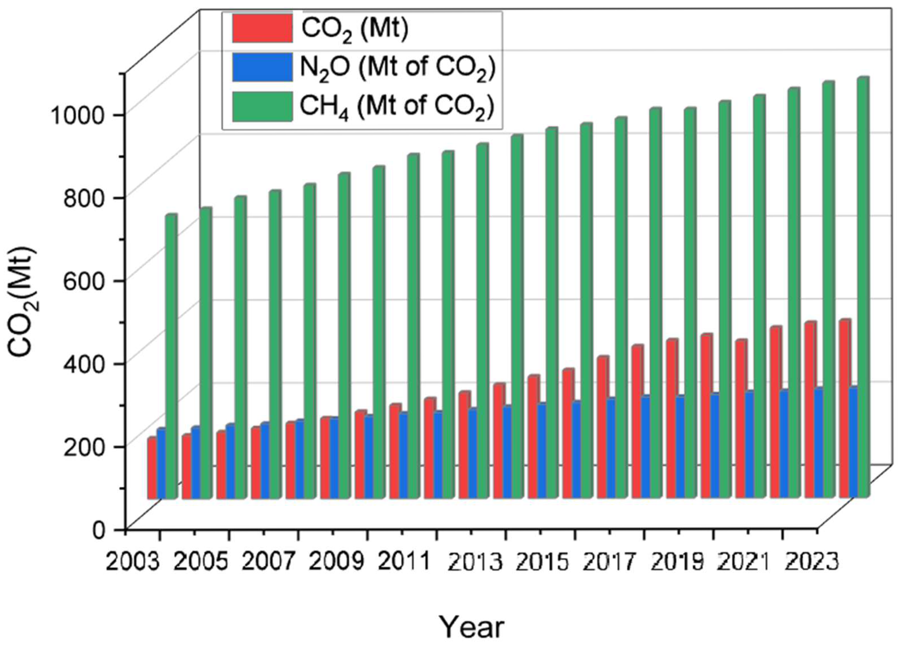
4.1. Preliminary Analysis—Trends

Figure 2 represents the total metric tons of carbon emissions, the total metric tons of CO₂ equivalent of methane and nitrous oxide emissions released annually from 2003 to 2023 in the least developed countries. A general trend observation indicates that the three greenhouse gases increase yearly. The only year the carbon emissions decreased was 2020, which can be attributed to the era of the coronavirus pandemic. The pandemic minimized industrial and human activities, leading to decreased CO₂ emissions. This reveals that efforts by governments and policymakers over the past few years to curb environmental pollution have not been efficient or effective. Therefore, more innovative studies are needed to determine the causal factors of GHGs and implement the necessary recommendations [7].

4.2. Descriptive Statistics, Multicollinearity, Unit Root, Cross-Sectional Dependency and Cointegration Tests

The study conducts a descriptive analysis before the diagnostic tests to examine fluctuations in the patterns of the selected variables. The analysis uses a dataset from 2003 to 2023, covering 81 developing countries. The descriptive analysis focuses on standard deviations, means, skewness and kurtosis based on 1701 observations (see

Table 2. Descriptive statistics.

Variables	Mean	Std Dev	Skewness	Kurtosis
CO2	0.019	0.086	8.529	80.844
N2O	0.043	0.124	5.757	39.128
CH4	0.042	0.113	5.573	38.329
FDI	0.122	0.064	8.226	83.435
REC	0.637	0.292	−0.559	2.104
FR	0.080	0.066	5.316	48.647
TOP	0.364	0.168	0.710	2.953
IND	0.367	0.150	1.539	6.067
POP	0.046	0.144	5.650	34.817
GOVS	0.302	0.132	1.419	7.398
GOVE	0.539	0.245	−0.036	2.033
GDP	0.017	0.069	10.109	120.872
OBS	1701

). The standard deviation values, ranging from 0.064 to 0.292, indicate that the data points are relatively close to the mean. Additionally, the selected indicators exhibit positive and negative skewness, suggesting that their distributions are significantly skewed to the left and right of the normal curve. Furthermore, the kurtosis values vary, with some indicators being less than three (platykurtic) and others exceeding three (leptokurtic), indicating a mix of distribution shapes. The unit root tests (ADF and IPS) are conducted to avoid spurious regression results (see

Table 3. Test results for multicollinearity, unit root and cross-sectional dependency.

Variables	VIF	CD	1st Difference
			ADF	IPS	PESCADF
CO2		111.89 ***	−3.440 ***	−19.605 ***	−4.388 ***
N2O		144.879 ***	−2.921 ***	−21.036 ***	−2.883 ***
CH4		78.793 ***	−6.687 ***	−18.602 ***	−3.257 ***
FDI	4.29	41.597 ***	−7.092 ***	−21.845 ***	−6.125 ***
REC	1.74	22.257 ***	−3.428 ***	−21.625 ***	−3.640 ***
FR	6.43	40.93 ***	−5.635 ***	−21.029 ***	−5.043 ***
TOP	1.50	35.811 ***	−6.118 ***	−18.698 ***	−3.287 ***
IND	1.22	26.187 ***	−4.604 ***	−18.852 ***	−3.429 ***
POP	2.48	138.764 ***	4.883 ***	23.210 ***	2.469 ***
GOVS	1.27	30.692 ***	−3.677 ***	−19.951 ***	−3.584 ***
GOVE	1.59	0.135	−3.474 ***	−21.199 ***	−4.545 ***
GDP	4.44	216.821 ***	−6.720 ***	−16.207 ***	−2.481 ***

*** denotes stationarity for unit root tests and the presence of significant cross-sectional dependency—VIF (Variance Inflation Factor); APF (augmented Dickey–Fuller); IPS (Im–Pesaran–Shin); CD (cross-sectional dependency); PESCADF (Pesaran’s cross-sectionally augmented Dickey–Fuller).

). The results reveal that the employed variables are stationary at first difference. Therefore, the Kao and Pedroni tests are carried out to determine the long-term relationship among the variables. The findings demonstrate that the variables are co-integrated (see

Table 4. Co-integration tests for developing countries.

Tests	Model 1 (CO2)	Model 2 (N2O)	Model 3 (CH4)
Kao test:
augmented Dickey–Fuller t	9.058 ***	−1.672 ***	9.414 ***
Pedroni test:
modified Phillips Perron t	11.962 ***	10.685 ***	11.398 ***
Phillips Perron t	−3.003 ***	−10.538 ***	−3.843 ***
Augmented Dickey–Fuller t	−2.534 ***	−9.296 ***	−4.255 ***

*** denotes all panels are cointegrated.

). Cross-sectional dependency is also considered in the cointegration test, and the null hypothesis of no cointegration is rejected, suggesting a relationship among the indicators (see Table 3). However, Pesaran’s cross-sectionally augmented Dickey–Fuller (PESCADF) handles the presence of cross-sectional dependency. Finally, the Variance Inflation Factor (VIF) is examined to detect multicollinearity among the independent variables (see Table 3). The analysis reveals that all VIF values are below the threshold of 10, indicating the absence of multicollinearity in this dataset.

4.3. General Group-Level Analysis

4.3.1. Regression Analysis for Developing Countries

From

Table 5. Linear regression analysis for developing countries.

Variables	Model 1 (CO2)		Model 2 (N2O)		Model 3 (CH4)
	FMOLS	CCR	FMOLS	CCR	FMOLS	CCR
C	0.139 *** (0.024)	0.139 *** (0.024)	−0.204 *** (0.026)	−0.204 *** (0.027)	−0.190 *** (0.032)	−0.190 *** (0.032)
FDI	−1.473 *** (0.214)	−1.465 *** (0.220)	1.959 *** (0.236)	1.964 *** (0.243)	1.780 *** (0.289)	1.783 *** (0.297)
REC	−0.288 *** (0.027)	−0.287 *** (0.028)	0.162 *** (0.030)	0.162 *** (0.031)	0.148 *** (0.037)	0.147 *** (0.037)
FR	2.745 *** (0.247)	2.740 *** (0.253)	−1.475 *** (0.272)	−1.478 *** (0.279)	−1.241 *** (0.332)	−1.243 *** (0.342)
TOP	−0.007 (0.011)	−0.006 (0.011)	−0.034 *** (0.012)	−0.034 *** (0.013)	−0.063 *** (0.015)	−0.063 *** (0.015)
IND	0.007 (0.011)	0.007 (0.012)	−0.003 (0.013)	−0.003 (0.013)	0.026 * (0.015)	0.026 * (0.016)
POP	0.233 *** (0.016)	0.232 *** (0.017)	0.570 *** (0.018)	0.569 *** (0.019)	0.464 *** (0.022)	0.463 *** (0.023)
GOVS	0.035 *** (0.013)	0.035 ** (0.014)	0.037 *** (0.015)	0.038 *** (0.015)	0.044 ** (0.018)	0.044 ** (0.019)
Obs.	1700
Sample	2003–2023
Cross-section	81

*, **, *** means significant at 10%, 5% and 1%, respectively.

, CCR and FMOLS models are employed using the STATA MP 17 software to analyze the linear nexus of FDI, REC and their synergy on environmental pollution (CO₂, N₂O and CH₄ emissions). Additionally, the clustered Pooled Least Square (PLS) is utilized as an alternative estimation technique to validate the findings (see

Table 6. Robustness test for the linear regression.

Variables	Model 1 (CO2)	Model 2 (N2O)	Model 3 (CH4)
C	0.151 *** (0.010)	−0.193 *** (0.010)	−0.178 *** (0.011)
FDI	−1.567 *** (0.091)	1.880 *** (0.087)	1.691 *** (0.096)
REC	−0.299 *** (0.012)	0.152 *** (0.011)	0.135 *** (0.122)
FR	2.828 *** (0.105)	−1.411 *** (0.100)	−1.158 *** (0.111)
TOP	−0.009 * (0.005)	−0.033 *** (0.005)	−0.058 *** (0.005)
IND	0.008 * (0.005)	−0.001 (0.005)	0.030 *** (0.005)
POP	0.241 *** (0.007)	0.576 *** (0.007)	0.465 *** (0.007)
GOVS	0.037 *** (0.006)	0.031 *** (0.005)	0.034 *** (0.006)

*, **, *** means significant at 10%, 5% and 1%, respectively.

). The results indicate that FDI significantly reduces CO₂ emissions, aligning with prior studies by Bello et al. [24] and Islam et al. [14]. This validates the pollution halo hypothesis for CO₂ emissions. However, FDI is found to increase N₂O and CH₄ emissions significantly (CCR, FMOLS, PLS: p < 0.001), consistent with the findings of Pazienza and De Lucia [8] and Mejia [48], who concluded that FDI expands N₂O and CH₄ emissions. This also confirms the pollution haven hypothesis for N₂O and CH₄ emissions. FDI often introduces advanced, energy-efficient and cleaner technologies to developing nations, particularly when investments originate from countries with stringent environmental standards. These technologies help reduce carbon emissions by enabling industries to adopt greener production methods and minimize energy waste. For example, Mercom [49] reports that India’s solar panel sector has received substantial funding from multinational companies aimed at lowering carbon intensity. However, its positive impact on N₂O and CH₄ emissions can be attributed to how foreign investments flow into energy-intensive and extractive industries, such as mining, oil extraction and agriculture, which are significant sources of methane and nitrous oxide emissions. These investments can directly contribute to higher emissions of both gases. For instance, Brazil has attracted substantial FDI in cattle ranching and dairy farming, increasing methane emissions due to the expansion of livestock numbers and intensive feeding practices.

Furthermore, REC shows a significant negative relation with CO₂ emissions and a positive correlation with N₂O and CH₄ emissions. This is congruent with the outcome of Zeeshan et al. [36], who indicated a negative interrelation between REC and CO₂ emissions. This result highlights that fossil fuel combustion releases large amounts of CO₂; however, when renewable energy systems are installed, they do not generally release CO₂ in their energy production process, especially wind, solar and hydro. India, for instance, has set a target of 175 GW of renewable energy capacity by 2022, facilitating the mitigation of emissions from the energy sector and ensuring an efficient energy transition. However, N₂O and CH₄ emissions can rise due to the decomposition of organic material in biomass, waste or hydropower projects. For example, large reservoirs formed by dams create ideal conditions for producing N₂O and CH₄ emissions. Organic materials such as trees and plants that get flooded can decompose anaerobically in the water, producing N₂O and CH₄ emissions. Moreover, the need for land to cultivate biofuels or bioenergy crops, such as corn, sugarcane, switchgrass, etc., can lead to deforestation or land-use changes, releasing methane and nitrous oxide. Deforestation, specifically in tropical regions, can release methane from wetland drainage and forest degradation. This can disrupt the natural carbon and nitrogen cycles, resulting in higher emissions of both N₂O and CH₄ emissions.

Moreover, results from the integration of FDI and REC demonstrate that it significantly increases CO₂ emissions but mitigates N₂O and CH₄ emissions. This shows that despite how REC aims to shift energy use toward cleaner sources, foreign investment in fossil fuel-intensive sectors such as oil extraction, coal mining and gas production can still increase carbon emissions due to exploration, extraction and transportation activities. Thus, foreign investments in the oil and gas sector in countries like Nigeria or Angola can increase carbon emissions from oil extraction, gas flaring and transportation of fossil fuels, despite efforts to expand renewable energy sources in the country. However, foreign investment in targeted technological improvements and cleaner practices, such as biogas systems and solar-powered irrigation, can replace diesel-powered equipment and mitigate N₂O and CH₄ emissions. For instance, Morocco has become a pioneer in solar energy development in Africa, particularly through the Noor Ouarzazate Solar Complex, one of the world’s largest solar power plants [50]. This project has attracted substantial FDI from international companies, including the World Bank, the European Investment Bank and ACWA Power, a Saudi Arabian-based company. This signifies a greater contribution to technological leapfrogging, resulting in a swift and more efficient energy transition and promoting agriculture and waste management to curb N₂O and CH₄ emissions. The outcome also validates that FDI in renewable energies supports the pollution halo effect for N₂O and CH₄ emissions. Therefore, H1 which suggests that integrating FDI and REC contribute to technological leapfrogging and validate the energy transition and pollution halo theories, mitigating environmental pollution, is confirmed for N₂O and CH₄ emissions but rejected for CO₂ emissions.

Finally, the outcomes of the control variables reveal that TOP statistically mitigates the three emissions, excluding CO₂, being insignificant. Industrialization increases CH₄ emissions and insignificantly relates to CO₂ and N₂O emissions. Population statistically intensifies the three emissions, validating the outcome of Donkor et al. [38], who revealed a positive correlation between population and N₂O emissions. GOVS consistently and statistically increase the three emissions, confirming the findings of Donkor et al. [38], who found a positive correlation between GOVS and CO₂ emissions.

4.3.2. Non-Linear Regression Analysis for Developing Countries

This research explores the non-linear influence of FDI, REC and their synergy on environmental pollution. The goal is to exhibit the threshold effects or turning points. The CCR and FMOLS techniques are utilized for the analysis (see

Table 7. Non-linear regression analysis for developing countries.

Variables	Model 1 (CO2)		Model 2 (N2O)		Model 3 (CH4)
	FMOLS	CCR	FMOLS	CCR	FMOLS	CCR
C	0.357 *** (0.071)	0.358 *** (0.077)	−0.246 *** (0.074)	−0.246 *** (0.080)	−0.203 ** (0.083)	−0.203 ** (0.089)
FDI	−3.927 *** (0.786)	−3.940 *** (0.852)	2.535 *** (0.814)	2.532 *** (0.880)	2.021 ** (0.915)	2.021 ** (0.990)
FDI2	3.882 *** (1.116)	3.920 *** (1.231)	−1.328 (1.156)	−1.310 (1.270)	−0.861 (1.299)	−0.865 (1.428)
REC	−0.580 *** (0.099)	−0.580 *** (0.106)	0.167 (0.102)	0.167 (0.110)	0.121 (0.115)	0.121 (0.123)
REC2	0.067 ** (0.027)	0.068 ** (0.029)	−0.002 (0.029)	−0.002 (0.030)	0.001 (0.032)	0.001 (0.033)
FR	5.426 *** (0.932)	5.437 *** (1.007)	−1.696 * (0.966)	−1.697 * (1.041)	−1.140 (1.086)	−1.135 (1.171)
FR2	−4.991 *** (1.505)	−5.031 *** (1.648)	1.159 * (1.558)	1.142 * (1.701)	0.626 (1.752)	0.626 (1.913)
TOP	−0.008 (0.012)	−0.007 (0.012)	−0.028 ** (0.012)	−0.028 ** (0.012)	−0.055 *** (0.014)	−0.055 *** (0.014)
IND	0.004 (0.013)	0.004 (0.013)	−0.005 (0.013)	−0.005 (0.013)	0.028 *** (0.015)	0.028 *** (0.015)
POP	0.248 *** (0.018)	0.247 *** (0.019)	0.556 *** (0.018)	0.556 *** (0.019)	0.453 *** (0.021)	0.452 *** (0.021)
GOVS	0.034 ** (0.014)	0.034 ** (0.014)	0.034 *** (0.014)	0.034 *** (0.015)	0.041 *** (0.016)	0.041 *** (0.017)
Obs.	1700
Sample	2003–2023
Cross-section	81

*, **, *** means significant at 10%, 5% and 1%, respectively.

), while the clustered PLS is employed for a robustness check in

Table 8. Robustness test for the non-linear regression.

Variables	Model 1 (CO2)	Model 2 (N2O)	Model 3 (CH4)
C	0.374 *** (0.028)	−0.231 *** (0.027)	0.199 *** (0.030)
FDI	−4.052 *** (0.313)	2.412 *** (0.296)	1.998 *** (0.334)
FDI2	3.947 *** (0.444)	−1.260 *** (0.420)	−0.824 * (0.474)
REC	−0.605 *** (0.039)	0.146 *** (0.037)	0.114 *** (0.042)
REC2	0.075 *** (0.011)	0.004 (0.010)	0.007 (0.012)
FR	5.556 *** (0.371)	−1.566 *** (0.351)	−1.146 *** (0.396)
FR2	−5.090 *** (0.598)	1.059 * (0.566)	0.603 (0.639)
TOP	−0.009 ** (0.005)	−0.029 *** (0.004)	−0.055 *** (0.005)
IND	0.005 (0.005)	−0.003 (0.005)	0.028 *** (0.005)
POP	0.255 *** (0.007)	0.563 *** (0.007)	0.455 *** (0.007)
GOVS	0.035 *** (0.006)	0.033 *** (0.005)	0.036 *** (0.006)

*, **, *** means significant at 10%, 5% and 1%, respectively.

. Table 7 and Table 8 reveal that the non-linear influence of FDI on CO₂ emissions has a U-shaped relationship, where initial investment reduces emissions but increases them after a certain point. This implies that, initially, developing countries can receive foreign investments in renewable energy technologies, such as solar, wind and hydropower. These technologies are typically less carbon-intensive than fossil fuel energy, thus promoting technological leapfrogging and the pollution halo theory in reducing carbon emissions. However, FDI leads to economic growth, and as the economy grows, the increase in demand for electricity, despite significant solar and wind energy investments, still leads to an increased reliance on coal-fired power plants and natural gas to meet demand.

Moreover, the outcomes of the nexus between REC and major GHGs reveal a U-shaped correlation with CO₂ emissions. This indicates that early adoption of renewable energy sources such as solar, wind, hydropower or bioenergy typically significantly reduces carbon emissions, as these sources produce little to no carbon dioxide compared to coal and oil. This ensures swift and efficient energy transition and encourages technological leapfrogging in mitigating CO₂ emissions. However, at the later stages, the lack of energy storage infrastructure, such as batteries or grid integration systems, can lead to inefficient use of renewable energy. For instance, when solar and wind power generation is high, but the demand is low, excess energy might be wasted. To balance this, energy systems may still rely on fossil fuels for stability and backup, leading to higher emissions.

Finally, synergizing FDI and REC indicate an inverted U-shaped relationship with CO₂, a U-shaped correlation with N₂O and an insignificant connection with CH₄ emissions. This implies that FDI often flows into developing countries to accelerate industrialization, which demands significant energy consumption. While FDI-driven projects in these nations typically involve resource extraction, heavy manufacturing and energy-intensive industries, their initial integration with renewable energy may not fully offset the high carbon emissions. However, as foreign investment increasingly targets technological leapfrogging, the pollution halo effect and a quality energy transition, there is a notable shift towards advanced renewable technologies such as solar, wind and hydropower. This transition gradually replaces coal and oil-based energy sources, mitigating carbon emissions. Moreover, with N₂O emissions, adopting cleaner technologies and renewable energy sources reduces reliance on fossil fuels, leading to robust energy transition and technological leapfrogging in reducing N₂O emissions. However, after reaching a certain threshold, the marginal benefits of additional investment and renewable energy deployment may diminish. This can occur due to grid integration challenges, intermittency of renewables and the need for fossil fuel backups. Hence, H2, which posits that synergizing FDI and REC reveals a U-shaped relation with environmental pollution in developing nations, is accepted for N₂O and rejected for CO₂ and CH₄ emissions.

4.3.3. Mediating Effect of Government Effectiveness and Economic Growth for Developing Countries

The outcome of the mediation effect model is demonstrated in

Table 9. Regression results of the mediation effects for developing countries.

	Mediation Effect of Government Effectiveness				Mediation Effect of Economic Growth
Variables	(1) GOVE	(2) CO2	(3) N2O	(4) CH4	(5) GDP	(6) CO2	(7) N2O	(8) CH4
GOVE		0.004 * (0.009)	0.008 * (0.009)	0.022 ** (0.011)
GDP						0.672 *** (0.039)	0.136 *** (0.051)	0.372 *** (0.058)
FDI	−3.687 * (2.607)	−1.452 *** (0.225)	1.996 *** (0.244)	1.851 *** (0.280)	0.054 * (0.095)	−1.532 *** (0.172)	1.942 *** (0.227)	1.701 *** (0.258)
REC	−0.855 *** (0.330)	−0.282 *** (0.029)	0.170 *** (0.031)	0.164 *** (0.036)	−0.080 *** (0.012)	−0.236 *** (0.022)	0.171 *** (0.029)	0.170 *** (0.033)
FR	3.615 * (3.005)	2.721 *** (0.260)	−1.512 *** (0.281)	−1.312 *** (0.322)	0.811 *** (0.109)	2.221 *** (0.201)	−1.574 *** (0.265)	−1.485 *** (0.301)
TOP	−0.435 *** (0.135)	−0.005 (0.012)	−0.030 ** (0.013)	−0.052 *** (0.015)	−0.018 *** (0.005)	0.006 (0.009)	−0.031 *** (0.012)	−0.055 *** (0.013)
IND	0.149 (0.140)	0.005 (0.012)	−0.005 (0.013)	0.024 * (0.015)	0.002 (0.005)	0.005 (0.009)	−0.005 (0.012)	0.027 *** (0.014)
POP	0.025 (0.201)	0.234 *** (0.017)	0.569 *** (0.019)	0.463 *** (0.021)	0.117 *** (0.007)	0.156 *** (0.014)	0.553 *** (0.019)	0.423 *** (0.021)
GOVS	−0.100 (0.163)	0.035 ** (0.014)	0.036 ** (0.015)	0.047 *** (0.017)	0.023 *** (0.006)	0.020 *** (0.011)	0.031 ** (0.014)	0.038 *** (0.016)
Obs.	1700
sample	2003–2023
cross-section	81

*, **, *** means significant at 10%, 5% and 1%, respectively.

using the FMOLS technique and in

Table 10. Robustness test of the mediation effects.

	Mediation Effect of Government Effectiveness				Mediation Effect of Economic Growth
Variables	(1) GOVE	(2) CO2	(3) N2O	(4) CH4	(5) GDP	(6) CO2	(7) N2O	(8) CH4
GOVE		0.004 * (0.009)	0.008 * (0.009)	0.022 ** (0.011)
GDP						0.669 *** (0.049)	0.132 ** (0.065)	0.372 *** (0.074)
FDI	−3.747 * (2.681)	−1.446 *** (0.233)	2.001 *** (0.252)	1.855 *** (0.288)	0.056 * (0.098)	−1.528 *** (0.177)	1.947 *** (0.233)	1.701 *** (0.266)
REC	−0.859 *** (0.338)	−0.282 *** (0.030)	0.170 *** (0.032)	0.165 *** (0.037)	−0.080 *** (0.012)	−0.236 *** (0.023)	0.171 *** (0.030)	0.170 *** (0.034)
FR	3.663 * (3.083)	2.717 *** (0.267)	−1.515 *** (0.289)	−1.315 *** (0.331)	0.810 *** (0.112)	2.221 *** (0.208)	−1.573 *** (0.274)	−1.484 *** (0.312)
TOP	−0.438 *** (0.139)	−0.005 (0.012)	−0.030 ** (0.013)	−0.052 *** (0.015)	−0.018 *** (0.005)	0.006 (0.009)	−0.031 *** (0.012)	−0.055 *** (0.013)
IND	0.151 (0.142)	0.005 (0.012)	−0.006 (0.013)	0.024 * (0.015)	0.002 (0.005)	0.005 (0.009)	−0.005 (0.012)	0.027 * (0.014)
POP	0.033 (0.209)	0.233 *** (0.018)	0.568 *** (0.019)	0.463 *** (0.022)	0.117 *** (0.008)	0.156 *** (0.014)	0.552 *** (0.019)	0.423 *** (0.022)
GOVS	−0.094 (0.168)	0.035 *** (0.015)	0.036 ** (0.016)	0.048 *** (0.018)	0.023 *** (0.006)	0.020 *** (0.011)	0.031 ** (0.014)	0.038 ** (0.017)
Obs.	1700
sample	2003–2023
cross-section	81

*, **, *** means significant at 10%, 5% and 1%, respectively.

employing the CCR method as a robustness test. Columns (1)–(4) reveal the mediation role of the core explanatory variables through GOVE. Specifically, the outcomes in column (1) in both Table 9 and Table 10 demonstrate that the regression coefficient of FDI on the mediating variable (GOVE) is negative, suggesting that an increment in FDI can create opportunities for multinational corporations to influence local government policies and regulations. This can result in regulatory capture, where governments become less effective at enforcing laws and regulations, particularly in areas such as environmental protection. Moreover, REC significantly decreases GOVE, indicating that the transition to renewable energy often requires complex regulatory adjustments and new administrative structures. Therefore, weak or inefficient institutions may struggle to manage these changes effectively, leading to inconsistencies or reductions in government effectiveness. However, the synergy of FDI and REC statistically increases GOVE, revealing that FDI often brings financial resources, advanced technology and international best practices. At the same time, REC projects require strong regulatory frameworks and efficient administration. This collaboration necessitates capacity building in institutions, promoting transparency, accountability and regulatory competence, which collectively enhance government effectiveness.

The outcome of the regression in Columns (2)–(4) for both Table 9 and Table 10 reveals that after introducing the mediating variable (GOVE), the regression coefficient of FDI remains significantly negative in its relationship with CO₂ and positive with N₂O and CH₄ emissions. Comparing the direct effect regression coefficient (−1.473), (1.959) and (1.780) of FDI on CO₂, N₂O and CH₄ emissions, respectively, in Table 5, it decreases to (−1.452) for CO₂ and rises to (1.996) and (1.851) for N₂O and CH₄ emissions, respectively. This indicates that GOVE plays a significant partial intermediary role in slowly mitigating CO₂ emissions. However, for N₂O and CH₄ emissions, GOVE is inefficient in curbing these emissions through FDI. Furthermore, the coefficient of REC is statistically negative for CO₂ and positive for N₂O and CH₄ emissions after introducing GOVE. The direct effect coefficient of REC on CO₂, N₂O and CH₄ emissions is (−0.288), (0.162) and (0.148), respectively; however, CO₂ emissions decrease to (−0.282) as N₂O and CH₄ emissions increase to (0.170) and (0.164) after introducing GOVE. This suggests that the GOVE in the developing nations is focused more on mitigating CO₂ emissions, neglecting the depleting effect of N₂O and CH₄ emissions. Furthermore, the impact of synergizing FDI and REC significantly remained positive for CO₂ emissions and negative for N₂O and CH₄ emissions. However, introducing GOVE slowly increases the coefficient of CO₂ to 2.721 and highly mitigates N₂O and CH₄ emissions to −1.512 and −1.312, respectively, compared with the outcome of the linear effects. This reveals that GOVE significantly mediates in highly reducing N₂O and CH₄ emissions through the synergy of FDI and REC. This enhances technological leapfrogging and validates the effects of the pollution halo and energy transition. Therefore, H3, which hypothesizes that GOVE, as a mediating variable, increases environmental pollution, is validated for CO₂ emissions and rejected for N₂O and CH₄ emissions.

The regression outcome of the mediation effect of FDI, REC and their synergy on environmental pollution through GDP is demonstrated in columns (5)–(8) (see Table 9 and Table 10). Specifically, the results in column (5) indicate that the regression coefficient of FDI on GDP is positive, indicating that an increase in FDI enhances GDP in developing nations. This suggests that as foreign companies invest in the developing nation’s industries, they enhance productivity, create employment and stimulate demand. This contributes to a higher output of goods and services, increasing GDP. Moreover, REC also significantly decreases GDP by 8%, indicating that the transition to renewable energy often involves significant upfront costs for infrastructure, technology and grid integration. Therefore, these high initial investments may strain government budgets and divert resources from other growth-enhancing sectors like education, healthcare or traditional infrastructure. However, synergizing FDI and REC statistically increases GDP in developing nations. This is due to how FDI brings capital and expertise to renewable energy projects requiring substantial initial investments. Suppose REC projects benefit from FDI’s ability to fund infrastructure like solar farms, wind turbines and advanced energy storage systems. In that case, it will spur economic activities and construct long-lasting economic growth.

The regression results in columns (6)–(8) (see Table 9 and Table 10) reveal that after introducing GDP as the mediating variable, the coefficient of FDI remains significantly positive with its relationship with N₂O and CH₄ emissions and negative with CO₂ emissions. A comparison with the direct effect regression coefficient in Table 5 shows GDP, as a mediating indicator, highly reduced CO₂ to −1.532 and slowly increased N₂O and CH₄ emissions to 1.942 and 1.701, respectively. This indicates that GDP is a significant intermediary in curbing the three emissions. Furthermore, the coefficient of REC is statistically negative for CO₂ and positive for N₂O and CH₄ emissions after introducing GDP. The direct effect coefficient of REC on CO₂, N₂O and CH₄ emissions is (−0.288), (0.162) and (0.148), respectively; however, CO₂ emissions decrease to (−0.236) as N₂O and CH₄ emissions increase to (0.171) and (0.170) after introducing GDP. This suggests that the economic growth in the developing nations slightly decreases CO₂ emissions; however, N₂O and CH₄ emissions are increased. Furthermore, the effect of synergizing FDI and REC significantly remains positive for CO₂ emissions and negative for N₂O and CH₄ emissions. Introducing GDP slowly increases the coefficient of CO₂ to 2.221 and highly mitigates N₂O and CH₄ emissions to −1.574 and −1.485, respectively. This demonstrates that GDP as a mediating factor slowly raises CO₂ emissions compared to the outcome in Table 5. Moreover, it facilitates technological leapfrogging and confirms the pollution halo and energy transition effect, as it highly curbs N₂O and CH₄ emissions through the synergy of FDI and REC. Hence, H4, which suggests that GDP, as a mediating variable, increases environmental pollution, is accepted for CO₂ emissions but rejected for N₂O and CH₄ emissions.

Finally, the outcomes in Table 9 and Table 10 reveal that the regression coefficient of GDP is significantly greater in mitigating environmental pollution than GOVE. The underlying reason is that as GDP increases due to the synergy of FDI and REC, it provides greater financial resources for pollution control and environmental initiatives than GOVE. These resources can directly fund renewable energy projects, green infrastructure and pollution mitigation strategies. Moreover, synergizing FDI and REC will amplify GDP growth, creating a feedback loop of increased investments, technological advancement and public–private sector engagement that yields faster and more substantial pollution reductions than government effectiveness alone.

4.4. Regional Variation Analysis

This study subdivides the 81 developing countries into income groups: LICs, MICs and HICs. This is to discover how the levels of economic growth shape the FDI–REC–pollution nexus. While HICs often leverage FDI for advanced green innovation, MICs grapple with balancing industrial expansion and renewable transitions, and low-income countries face structural barriers to attracting sustainable investment. Therefore, this regional differentiation is critical to moving beyond one-size-fits-all solutions, offering tailored insights for policymakers to harness FDI-REC synergies in alignment with local economic and environmental realities.

4.4.1. Linear Regression of the Regional Variation

Table 11. Linear regression analysis for the regional variations.

Variables	Model 1 (CO2)		Model 2 (N2O)		Model 3 (CH4)
	FMOLS	CCR	FMOLS	CCR	FMOLS	CCR
Low-income countries
FDI	0.089 (0.085)	0.106 (0.093)	−0.304 *** (0.083)	−0.307 *** (0.090)	−0.300 *** (0.063)	−0.299 *** (0.069)
REC	0.456 *** (0.057)	0.460 *** (0.060)	−0.071 * (0.056)	−0.074 * (0.058)	−0.092 ** (0.043)	−0.094 ** (0.044)
FR	1.356 *** (0.253)	1.326 *** (0.271)	2.668 *** (0.249)	2.685 *** (0.261)	2.576 *** (0.332)	2.587 *** (0.199)
TOP	−0.362 *** (0.055)	−0.359 *** (0.060)	−0.216 *** (0.053)	−0.212 *** (0.056)	−0.160 *** (0.041)	−0.156 *** (0.043)
IND	−0.067 (0.049)	−0.074 (0.052)	−0.083 * (0.048)	−0.083 * (0.050)	−0.044 (0.036)	−0.046 (0.038)
POP	0.570 *** (0.059)	0.563 *** (0.062)	1.052 *** (0.058)	1.053 *** (0.061)	1.074 *** (0.022)	1.072 *** (0.046)
GOVS	−0.068 * (0.039)	−0.070 * (0.042)	0.020 (0.038)	0.021 (0.041)	0.159 (0.029)	0.016 (0.031)
Middle-income countries
FDI	−1.533 *** (0.247)	−1.528 *** (0.254)	2.035 *** (0.299)	2.043 *** (0.307)	1.849 *** (0.301)	1.855 *** (0.310)
REC	−0.292 *** (0.032)	−0.292 *** (0.033)	0.178 *** (0.039)	0.178 *** (0.040)	0.165 *** (0.039)	0.165 *** (0.040)
FR	2.813 *** (0.284)	2.810 *** (0.291)	−1.553 *** (0.343)	−1.559 *** (0.352)	−1.307 *** (0.346)	−1.310 *** (0.356)
TOP	−0.007 (0.014)	−0.007 (0.015)	−0.030 * (0.017)	−0.029 * (0.018)	−0.063 *** (0.017)	−0.063 *** (0.018)
IND	0.003 (0.018)	0.003 (0.018)	0.014 (0.021)	0.013 (0.022)	0.058 *** (0.022)	0.058 *** (0.022)
POP	0.231 *** (0.019)	0.230 *** (0.020)	0.559 *** (0.023)	0.558 *** (0.024)	0.442 *** (0.023)	0.441 *** (0.024)
GOVS	0.040 *** (0.017)	0.040 *** (0.018)	0.039 * (0.021)	0.039 * (0.022)	0.052 ** (0.021)	0.051 *** (0.022)
High-income countries
FDI	−1.643 *** (0.471)	−1.780 *** (0.549)	−0.235 * (0.451)	−0.213 * (0.511)	−1.886 *** (0.564)	−2.059 *** (0.656)
REC	−0.303 * (0.172)	−0.334 * (0.194)	−0.282 * (0.165)	−0.286 * (0.184)	−0.386 ** (0.206)	−0.427 ** (0.233)
FR	2.049 *** (0.645)	2.249 *** (0.778)	0.482 * (0.617)	0.469 * (0.726)	2.254 *** (0.772)	2.501 *** (0.932)
TOP	−0.026 (0.085)	−0.032 (0.088)	0.148 * (0.081)	0.150 * (0.084)	−0.141 (0.101)	−0.147 (0.105)
IND	0.165 (0.116)	0.166 (0.122)	0.005 (0.111)	0.014 (0.116)	0.307 ** (0.139)	0.309 (0.146)
POP	0.618 *** (0.093)	0.609 *** (0.102)	0.771 *** (0.089)	0.771 *** (0.097)	0.531 *** (0.111)	0.522 *** (0.122)
GOVS	0.200 *** (0.087)	0.196 ** (0.091)	−0.067 (0.084)	−0.067 (0.041)	0.054 (0.104)	0.048 (0.109)

*, **, *** means significant at 10%, 5% and 1%, respectively.

and

Table 12. Robustness test for linear relationship.

Variables	Low-Income Countries			Middle-Income Countries			High-Income Countries
	Model 1 (CO2)	Model 2 (N2O)	Model 3 (CH4)	Model 1 (CO2)	Model 2 (N2O)	Model 3 (CH4)	Model 1 (CO2)	Model 2 (N2O)	Model 3 (CH4)
FDI	−0.078 (0.074)	−0.207 *** (0.054)	−0.244 *** (0.050)	−1.566 *** (0.112)	1.987 *** (0.103)	1.818 *** (0.114)	−1.289 *** (0.167)	−0.189 (0.155)	−1.412 *** (0.204)
REC	0.330 *** (0.053)	−0.015 (0.039)	−0.048 (0.036)	−0.299 *** (0.051)	0.170 *** (0.013)	0.156 *** (0.015)	−0.230 *** (0.062)	−0.297 *** (0.057)	−0.274 *** (0.074)
FR	1.895 *** (0.223)	2.340 *** (0.164)	2.388 *** (0.151)	2.845 *** (0.128)	−1.515 *** (0.119)	−1.281 *** (0.131)	1.547 *** (0.230)	0.463 *** (0.213)	1.594 *** (0.208)
TOP	−0.289 *** (0.048)	−0.211 *** (0.035)	−0.156 *** (0.032)	−0.010 (0.007)	−0.038 *** (0.006)	−0.069 *** (0.007)	0.008 (0.032)	0.143 *** (0.029)	−0.111 *** (0.039)
IND	−0.078 * (0.042)	−0.097 *** (0.031)	−0.056 ** (0.028)	0.009 (0.008)	0.022 *** (0.007)	0.062 *** (0.008)	0.155 *** (0.043)	0.064 * (0.040)	0.304 *** (0.052)
POP	0.599 *** (0.050)	1.036 *** (0.036)	1.070 *** (0.034)	0.234 *** (0.009)	0.564 *** (0.008)	0.446 *** (0.009)	0.651 *** (0.033)	0.785 *** (0.031)	0.582 *** (0.040)
GOVS	−0.128 *** (0.036)	0.028 (0.026)	0.028 (0.024)	0.042 *** (0.008)	0.045 *** (0.007)	0.051 *** (0.008)	0.192 *** (0.033)	−0.023 (0.030)	0.009 (0.040)

*, **, *** means significant at 10%, 5% and 1%, respectively.

indicate the linear nexus of FDI, REC and their synergy on environmental pollution for LICs, MICs and HICs. CCR and FMOLS models are chosen for the analysis (see Table 11), and the clustered Pooled Least Square (PLS) is employed as an alternative estimation technique to validate the findings (see Table 12). Outcomes from the LICs reveal that FDI and REC individually increase CO₂ and reduce N₂O and CH₄ emissions; however, FDI’s interrelationship with CO₂ emissions is insignificant. This suggests that in LICs, a significant portion of FDI often targets sectors like agriculture, raw material extraction and services rather than energy-intensive industrial manufacturing. These sectors contribute less to CO₂ emissions compared to heavy industry. However, FDI may promote modern agricultural practices that use fertilizers and waste management systems more efficiently, thereby reducing N₂O and CH₄ emissions and promoting the halo effect theory in LICs. Moreover, renewable energy projects often expand electricity access to underserved areas, increasing total energy demand and consumption. Therefore, though renewables contribute clean energy, the parallel use of fossil fuels for reliability can raise CO₂ emission. However, solar and biogas systems are increasingly used to manage organic waste in LICs. These technologies directly reduce N₂O and CH₄ emissions by improving waste decomposition processes, encouraging an efficient energy transition. Furthermore, synergizing FDI and REC intensifies the three emissions in low-income countries. This reveals that the integration often results in economic expansion, which can significantly raise the demand for energy, agricultural products and infrastructure. While REC mitigates emissions in some sectors, the overall increase in energy demand, industrial activity and agricultural expansion may lead to higher emissions of CO₂, N₂O and CH₄, especially in the transition phase, where fossil fuel use remains dominant. Therefore, H1 is rejected for the three emissions in LICs.

Results from the MICs show that FDI and REC individually curb CO₂ and raise N₂O and CH₄ emissions. This demonstrates that FDI in MICs often promotes advanced, energy-efficient and cleaner technologies, reducing CO₂ emissions. However, FDI into energy-intensive and extractive industries, such as mining, oil extraction and agriculture, which are major sources of N₂O and CH₄ emissions, can intensify these GHGs. Moreover, REC in MICs enables more energy-efficient systems, such as decentralized solar installations or mini-grids, which reduce reliance on coal and gas plants, significantly curbing CO₂ emissions. However, renewable energy infrastructure in MICs often lacks advanced methane-capture systems or fertilizer-management technologies. This inefficiency exacerbates CH₄ and N₂O emissions during the transition to renewable energy. Furthermore, integrating FDI and REC mitigates N₂O and CH₄ emissions but expands CO₂ emissions. This suggests that FDI stimulates economic activity, infrastructure development and industrial expansion, which increase energy demand. This higher energy demand often exceeds renewable energy supply, necessitating fossil fuel use to meet the shortfall, increasing CO₂ emissions. However, FDI combined with renewable energy systems enables the adoption of precision farming techniques that optimize fertilizer use, significantly reducing N₂O emissions. Therefore, H1, which posits that synergizing FDI and REC contributes to technological leapfrogging and validates the energy transition and pollution halo theories, mitigating environmental pollution, is confirmed for N₂O and CH₄ emissions but rejected for CO₂ emissions in MICs.

Findings from the HICs reveal that FDI and REC individually mitigate the three emissions. This asserts that strong environmental policies and enforcement in high-income countries compel foreign investors to adopt cleaner technologies and comply with emissions standards, reducing these emissions and enhancing the halo effect theories. Moreover, HICs leverage cutting-edge renewable energy technologies and set environmental policies that optimize energy production and minimize associated emissions across CO₂, N₂O and CH₄ emissions, thus encouraging efficient energy transition. However, synergizing FDI and REC expands these emissions in HICs, suggesting that the policies incentivizing FDI and REC may not fully align with stringent environmental goals, leading to unintended increases in emissions. Additionally, FDI investors often prioritize returns, which might lead to cutting corners on sustainable practices or focusing on short-term gains that compromise long-term emission reduction goals. Therefore, H1 is rejected for the three emissions in HICs.

4.4.2. Non-Linear Regression of the Regional Variation

This paper investigates the non-linear nexus of FDI, REC and their synergy on environmental pollution for low-, middle- and high-income countries, (see

Table 13. Non-linear regression analysis for the regional variations.

Variables	Model 1 (CO2)		Model 2 (N2O)		Model 3 (CH4)
	FMOLS	CCR	FMOLS	CCR	FMOLS	CCR
Low-income countries
FDI	0.200 (0.368)	0.246 (0.432)	−0.630 *** (0.207)	−0.674 *** (0.242)	−0.549 *** (0.190)	−0.589 *** (0.069)
FDI2	−0.101 (0.287)	−0.121 (0.337)	0.280 * (0.162)	0.314 * (0.190)	0.193 (0.149)	0.225 (0.174)
REC	0.806 *** (0.301)	0.788 ** (0.352)	0.282 * (0.170)	0.230 * (0.197)	0.190 ** (0.156)	0.134 ** (0.044)
REC2	−0.409 * (0.234)	−0.380 * (0.260)	−0.479 *** (0.132)	−0.446 *** (0.146)	−0.383 (0.121)	−0.346 (0.133)
FR	0.839 (1.411)	0.748 (1.753)	3.712 *** (0.795)	3.967 *** (0.261)	3.444 *** (0.730)	3.695 *** (0.890)
FR2	1.983 (3.768)	2.225 (4.695)	−4.267 ** (2.123)	−4.886 * (2.615)	−3.307 * (1.949)	−3.896 * (2.390)
TOP	−0.388 *** (0.085)	−0.373 *** (0.090)	−0.293 *** (0.048)	−0.285 *** (0.050)	−0.216 *** (0.044)	−0.207 *** (0.046)
IND	−0.062 (0.075)	−0.071 (0.080)	−0.058 (0.042)	−0.058 (0.045)	−0.017 (0.039)	−0.018 (0.041)
POP	0.590 *** (0.089)	0.581 *** (0.095)	1.093 *** (0.050)	1.090 *** (0.053)	1.121 *** (0.046)	1.116 *** (0.049)
GOVS	−0.101 * (0.061)	−0.097 * (0.065)	−0.024 (0.034)	−0.024 (0.037)	−0.009 (0.031)	−0.009 (0.034)
Middle-income countries
FDI	−4.327 *** (0.643)	−4.328 *** (0.695)	2.543 *** (0.538)	2.542 *** (0.580)	2.284 *** (0.699)	2.282 *** (0.754)
FDI2	4.199 *** (0.902)	4.203 *** (0.995)	−1.464 ** (0.755)	−1.461 ** (0.828)	−1.230 (0.981)	−1.225 (1.077)
REC	−0.657 *** (0.082)	−0.656 *** (0.088)	0.159 ** (0.069)	0.159 *** (0.074)	0.141 (0.090)	0.141 (0.096)
REC2	0.089 *** (0.027)	0.089 *** (0.027)	−0.002 (0.022)	−0.003 (0.023)	0.001 (0.029)	0.001 (0.029)
FR	5.962 *** (0.762)	5.961 *** (0.821)	−1.600 *** (0.637)	−1.600 *** (0.685)	−1.319 (0.828)	−1.316 (0.890)
FR2	−5.521 *** (1.210)	−5.524 *** (1.324)	1.194 (1.013)	1.191 (1.014)	0.966 (1.316)	0.958 (1.435)
TOP	−0.013 (0.010)	−0.013 (0.011)	−0.033 *** (0.009)	−0.033 *** (0.009)	−0.063 *** (0.017)	−0.063 *** (0.018)
IND	0.004 (0.013)	0.003 (0.018)	0.015 (0.011)	0.015 (0.011)	0.058 *** (0.022)	0.058 *** (0.022)
POP	0.250 *** (0.014)	0.250 *** (0.015)	0.548 *** (0.012)	0.548 *** (0.013)	0.430 *** (0.016)	0.430 *** (0.016)
GOVS	0.043 *** (0.013)	0.043 *** (0.013)	0.046 *** (0.011)	0.046 *** (0.011)	0.049 *** (0.014)	0.049 *** (0.014)
High-income countries
FDI	−0.380 *** (0.918)	−0.767 (1.413)	−0.783 (0.931)	−0.666 (1.432)	−0.205 (1.082)	−0.739 (1.661)
FDI2	−0.596 (0.729)	−0.376 (1.061)	0.769 (0.739)	0.719 (1.077)	−0.633 (0.859)	−0.3168 (1.249)
REC	−0.717 ** (0.303)	−0.811 ** (0.389)	−0.527 * (0.308)	−0.286 * (0.184)	−1.256 *** (0.358)	−1.377 *** (0.459)
REC2	0.587 *** (0.209)	0.599 *** (0.220)	0.219 (0.212)	0.482 (0.394)	1.110 *** (0.246)	1.125 *** (0.258)
FR	0.447 (1.296)	1.042 (1.977)	0.759 (1.314)	0.531 (2.005)	−0.095 (1.527)	0.666 (2.324)
FR2	0.939 (1.273)	0.466 (1.868)	−0.696 (0.290)	−0.520 (1.898)	1.276 (1.500)	0.673 (0.199)
TOP	0.026 (0.068)	0.020 (0.071)	0.138 ** (0.069)	0.140 ** (0.072)	−0.070 (0.080)	−0.077 (0.083)
IND	0.008 (0.109)	0.012 (0.116)	−0.042 (0.110)	−0.042 (0.117)	0.014 (0.128)	0.017 (0.136)
POP	0.652 *** (0.076)	0.642 *** (0.085)	0.801 *** (0.077)	0.808 *** (0.085)	0.607 *** (0.089)	0.598 *** (0.100)
GOVS	0.189 *** (0.070)	0.190 *** (0.073)	−0.038 (0.070)	−0.040 (0.074)	0.049 (0.082)	0.049 (0.085)

*, **, *** means significant at 10%, 5% and 1%, respectively.

and

Table 14. Robustness test for the non-linear regression.

Variables	Low-Income Countries			Middle-Income Countries			High-Income Countries
	Model 1 (CO2)	Model 2 (N2O)	Model 3 (CH4)	Model 1 (CO2)	Model 2 (N2O)	Model 3 (CH4)	Model 1 (CO2)	Model 2 (N2O)	Model 3 (CH4)
FDI	−0.029 (0.224)	−0.320 ** (0.145)	−0.288 ** (0.137)	−4.292 *** (0.388)	0.289 *** (0.351)	2.404 *** (0.396)	−0.199 (0.039)	−0.621 * (0.380)	0.082 (0.433)
FDI2	−0.023 (0.174)	0.085 (0.113)	0.024 (0.107)	4.155 *** (0.545)	−1.641 *** (0.493)	−1.398 ** (0.555)	−0.582 * (0.314)	0.626 ** (0.299)	−0.608 * (0.340)
REC	0.685 *** (0.181)	0.474 *** (0.117)	0.388 *** (0.111)	−0.671 *** (0.050)	0.166 *** (0.045)	0.151 *** (0.051)	−0.552 *** (0.130)	−0.715 *** (0.124)	−1.053 *** (0.141)
REC2	−0.340 ** (0.135)	−0.549 *** (0.087)	−0.477 *** (0.082)	0.099 *** (0.016)	0.001 (0.014)	0.001 (0.016)	0.508 *** (0.089)	0.371 *** (0.085)	1.030 *** (0.096)
FR	1.394 * (0.846)	2.585 *** (0.547)	2.505 *** (0.517)	5.944 *** (0.460)	−1.740 *** (0.416)	−1.445 *** (0.468)	−0.027 (0.564)	0.838 (0.537)	−0.592 (0.612)
FR2	0.603 (2.232)	−2.282 * (1.443)	−1.832 (1.365)	−5.483 *** (0.730)	1.408 ** (0.661)	1.180 * (0.744)	1.207 ** (0.553)	−0.762 (0.526)	1.385 ** (0.600)
TOP	−0.336 *** (0.050)	−0.295 *** (0.033)	−0.228 *** (0.031)	0.011 * (0.006)	−0.033 *** (0.006)	−0.064 *** (0.006)	0.040 *** (0.030)	0.153 *** (0.029)	−0.053 (0.033)
IND	−0.067 (0.043)	−0.068 ** (0.028)	−0.034 (0.027)	0.007 (0.008)	0.016 ** (0.007)	0.057 *** (0.008)	−0.003 (0.048)	−0.045 (0.045)	−0.007 (0.052)
POP	0.634 *** (0.051)	1.096 *** (0.032)	1.120 *** (0.031)	0.248 *** (0.009)	0.544 *** (0.007)	0.429 *** (0.009)	0.674 *** (0.032)	0.800 *** (0.031)	0.623 *** (0.035)
GOVS	−0.138 *** (0.037)	−0.005 (0.024)	0.002 (0.023)	0.045 *** (0.008)	0.048 *** (0.007)	0.054 *** (0.008)	0.198 *** (0.031)	−0.017 (0.030)	0.026 (0.034)

*, **, *** means significant at 10%, 5% and 1%, respectively

). The findings from Table 13 and Table 14 demonstrate that in LICs, FDI has a U-shaped relationship with N₂O and an insignificant correlation with CO₂ and CH₄ emissions. This reveals that initial investment reduces N₂O emissions but increases after a certain point. At low levels of FDI, investments in LICs are often directed toward modernizing agriculture and infrastructure through the introduction of efficient agricultural techniques, such as precision agriculture, mitigating N₂O emissions. However, over time, weak regulatory frameworks in LICs often fail to manage the environmental impact of large-scale FDI projects, allowing emissions to rise unchecked. Furthermore, REC shows an inverted U-shaped connection with the three emissions. This indicates that initially, REC helps reduce emissions, as it displaces traditional, carbon-intensive energy sources like biomass and coal. This early stage focuses on cleaner energy and energy efficiency improvements, leading to emission reductions. However, as the demand for energy rises, and LICs scale up bioenergy or other renewable energy projects, increased fertilizer use, inefficient energy systems and early-stage infrastructure challenges can lead to higher emissions, temporarily. Meanwhile, synergizing FDI and REC has a U-shaped relationship with the three emissions. This implies that while emissions rise initially due to industrial and agricultural expansion, FDI can continually ensure the use of modern, low-emission technologies that complement renewable energy adoption, enabling LICs to reduce emissions in the agriculture, industry and energy sectors. Hence, H2, which posits that synergizing FDI and REC reveals a U-shaped relationship with environmental pollution in developing nations, is accepted for the three emissions in LICs.

The results from the MICs also reveal that FDI has a U-shaped nexus with CO₂, an inverted U-shaped interrelation with N₂O emissions and an insignificant correlation with CH₄ emissions. This suggests that CO₂ emissions initially decrease with FDI but increase after a turning point. This can be attributed to energy efficiency gains where, initially, FDI brings in more energy-efficient industrial technologies, cleaner production methods and better energy utilization practices, helping to reduce CO₂ emissions. Notwithstanding, as FDI matures, investment begins to target heavy industries and energy-intensive sectors, leading to increased energy consumption and a rise in CO₂ emissions. Moreover, in MICs, FDI often supports agricultural expansion to meet export demands. This leads to increased use of nitrogen-based fertilizers, increasing N₂O emissions. However, as FDI grows, it introduces more modern and sustainable agricultural practices, with a gradual adoption. This leads to a plateau in emissions as some regions or sectors begin to implement better management practices. REC also reveals a U-shaped interrelation with CO₂ and an insignificant connection with N₂O and CH₄ emissions. This asserts that renewable energy sources such as solar, wind and hydro begin to displace fossil fuels like coal and oil in power generation, leading to a reduction in CO₂ emissions. Notwithstanding, as MICs grow economically, energy demand increases, often outpacing the capacity of renewable energy systems. This creates pressure to revert to fossil fuels for meeting additional demand. Furthermore, integrating FDI and REC demonstrates an inverted U-shaped relationship with CO₂ emissions and an insignificant nexus with N₂O and CH₄ emissions. This reflects the transitional nature of FDI and REC synergy in MICs. While emissions may initially rise due to industrial expansion and energy infrastructure limitations, they eventually decline as renewable energy systems mature, policies strengthen, and FDI aligns with sustainable development objectives. Therefore, H2 is rejected for the three emissions in MICs.

Finally, from the HICs, FDI and the synergy of FDI and REC indicate an insignificant non-linear relationship with the three emissions. This suggests a balanced dynamic where the combined effects of FDI and REC neither significantly increase nor reduce CO₂ emissions in high-income countries. This outcome is due to advanced renewable energy adoption, stringent environmental regulations and a mature decarbonized economic structure that minimizes emissions variability. However, REC shows a U-shaped correlation with CO₂ emissions and an insignificant nexus with N₂O and CH₄ emissions. This asserts that governments in HICs typically support REC through subsidies, tax incentives and regulations, accelerating the transition to low-carbon energy sources. However, as the share of renewables grows, their intermittent nature, such as in solar and wind, creates challenges in meeting continuous energy demand, leading to reliance on backup fossil fuel-based power plants. Thus, H2 is rejected for the three emissions in HICs (see Table 13 and Table 14).

5. Conclusions, Implication and Recommendation

5.1. Conclusions

This study ascertains how FDI and REC can be synergized to promote technological leapfrogging, contributing to environmental pollution mitigation through theoretical and empirical approaches. The research focuses on 81 developing countries, analyzing them on general group and regional variation (LICS, MICs and HICs) levels. The CCR, FMOLS and clustered PLS methods are used to analyze the study data from 2003 to 2023 to ensure robust results. Diagnostic tests, including multicollinearity (VIF), unit root, cointegration and cross-sectional dependence tests, are conducted to prevent spurious results and validate the interrelations among the selected indicators. The outcomes reveal no spurious results and multicollinearity among the variables. This research tested the following hypotheses: (i) H1: Synergizing FDI and REC contributes to technological leapfrogging and validates the pollution halo and energy transition theories, mitigating environmental pollution in developing nations. (ii) H2: Synergizing FDI and REC reveals a U-shaped relationship with environmental pollution in developing nations. (iii) H3: Government effectiveness, as a mediating variable for the synergy of FDI and REC, significantly increases developing nations’ environmental pollution. (iv) H4: Economic growth, as a mediating variable for the synergy of FDI and REC, significantly increases environmental pollution in developing nations. The tested hypotheses’ outcomes demonstrate that at the general group level, H1 is validated for only N₂O and CH₄ emissions, H3 and H4 are confirmed for only CO₂ emissions, and H2 is rejected for CO₂ and CH₄ emissions. Moreover, at the regional variation level, H1 is rejected for the three emissions in LICs and HICs but accepted for N₂O and CH₄ emissions in MICs. Additionally, H2 is rejected for the three emissions in LICS, MICs and HICs. The study analyzed the linear, non-linear and mediating effects among the chosen variables. However, the findings highlight more robust linear effects of the integration of FDI and REC in environmental pollution mitigation.

The regression results from the linear correlation analysis of FDI, REC and their synergy on GHGs demonstrate that FDI and REC significantly mitigate CO₂ emissions but intensify N₂O and CH₄ emissions. However, their synergy significantly increases CO₂ emissions but curbs N₂O and CH₄ emissions, validating the pollution halo and energy transition theories and enhancing technological leapfrogging for N₂O and CH₄ emissions. The control variables reveal that TOP mitigates the three emissions, with CO₂ being insignificant. Also, industrialization significantly increases CH₄ emissions. POP and GOVS significantly intensify all the three emissions. Moreover, the findings from the non-linear impact of FDI, REC and their synergy show that FDI and REC have a significant, U-shaped effect on CO₂ emissions. However, their synergy demonstrates an inverted U-shaped nexus with CO₂ and a U-shaped correlation with N₂O emissions. Furthermore, the regression results of the indirect effect of FDI, REC and their synergy, using government effectiveness and economic growth as the mediating variables, remained consistent with the outcome of the linear relationship. This suggests that the direct and indirect effects of FDI, REC and their synergy are consistent in mitigating environmental pollution in developing nations. However, the mediating effect of GDP surpasses that of GOVE in curbing environmental pollution. This makes GDP a key channel through which FDI and REC can effectively use to ensure environmental sustainability.

Findings of the linear regressions from the regional variations indicate that in LICs, FDI and REC individually intensify CO₂ and reduces N₂O and CH₄ emissions. However, synergizing FDI and REC increases the three emissions. Additionally, in MICs, FDI and REC individually mitigate CO₂ and raise N₂O and CH₄ emissions; notwithstanding, integrating FDI and REC reduces N₂O and CH₄ emissions but expands CO₂ emissions. Moreover, in HICs, FDI and REC individually reduce the three emissions. However, synergizing FDI and REC expands these emissions. Results from the non-linear analysis reveal that FDI has a U-shaped relationship with N₂O and an insignificant correlation with CO₂ and CH₄ emissions in LICs. REC also shows an inverted U-shaped connection with the three emissions. However, synergizing FDI and REC has a U-shaped relationship with the three emissions. In MICs, FDI has a U-shaped connection with CO₂, an inverted U-shaped interrelation with N₂O emissions and an insignificant correlation with CH₄ emissions. REC also shows a U-shaped interrelation with CO₂ and an insignificant connection with N₂O and CH₄ emissions. Notwithstanding, integrating FDI and REC demonstrates an inverted U-shaped relationship with CO₂ emissions and an insignificant nexus with N₂O and CH₄ emissions. Finally, in HICs, FDI and the synergy of FDI and REC indicate an insignificant non-linear relationship with the three emissions. However, REC shows a U-shaped correlation with CO₂ emissions and an insignificant nexus with N₂O and CH₄ emissions.

5.2. Theoretical Implication of the Study

The outcomes of this research correlate with the concept of technological leapfrogging, where nations, particularly developing ones, forgo intermediate or traditional stages of technological development and directly adopt advanced, modern technologies. This concept also corroborates with pollution halo and energy transition theories to ensure environmental pollution mitigation in developing nations. Results from the group level and MICs reveal that synergizing FDI and REC has a negative interrelation with N₂O and CH₄ emissions. This supports the notion that foreign investment in renewable energies will bypass outmoded or intermediate tools and accelerate the adoption of advanced technologies, thereby influencing a faster and more efficient energy transition in mitigating environmental pollution in developing nations. Moreover, mediating government effectiveness and economic growth with the correlation between the synergy of FDI and REC and environmental pollution shows that it reduces N₂O and CH₄ emissions. This also corroborates technology leapfrogging and validates pollution halo and energy transition theories.

5.3. Practical Implication of the Study

This paper’s practical implications are beneficial for policymakers, government and stakeholders. The outcomes offer insightful and effective policies and strategies by elucidating the role of synergizing FDI and REC in environmental pollution mitigation. The insights guide policymakers in policy development to attract FDI to support renewable energy projects in environmental pollution mitigation. Additionally, stakeholders are enlightened in investment decisions for foreign investors and local businesses. Moreover, government and policymakers are guided to design policies to encourage technology transfer from foreign investors, enabling faster adoption of green technologies and stimulating local innovation in the renewable energy sector. Finally, this insight also creates an urgency to develop regional policy alliances to jointly tackle environmental pollution through FDI and renewable energy, benefiting from shared infrastructure and knowledge transfer.

5.4. Recommendations

Based on the outcomes of this research, this study lays out the following suggestions:

Firstly, about the direct influence of FDI increasing N₂O and CH₄ emissions and decreasing CO₂ emissions at both the group level and in MICs, governments and policymakers should encourage FDI in sectors that utilize low-emission technologies, particularly in agriculture and waste management, where nitrous oxide and methane are prevalent. This can involve creating incentives for foreign companies that invest in innovative practices or technologies that reduce N₂O and CH₄ emissions. Moreover, sustainable farming practices that minimize nitrous oxide emissions, such as precision agriculture, improved fertilizer application techniques and crop rotation, should be promoted. These policies will mitigate the increase in these GHGs as they also sustain the reduction in CO₂ emissions.

Secondly, results also reveal that REC at both the group level and in MICs increases N₂O and CH₄ emissions and decreases CO₂ emissions; therefore, policymakers should modify the renewable energy portfolio to include sources with the lowest N₂O and CH₄ footprints, such as wind, solar and modernized biomass technologies. Different renewable energy sources have distinct effects on these emissions. Therefore, a balanced mix can reduce the total N₂O and CH₄ emissions. The government should also require comprehensive lifecycle assessments (LCAs) for renewable energy projects to ascertain their total environmental effect, thus, N₂O and CH₄ emissions. LCAs can determine phases in the renewable energy lifecycle where emissions peak and allow for targeted interventions to curb N₂O and CH₄ emissions. This can counteract the higher emissions from one renewable source with the lower emissions from another to create a more balanced environmental outcome.

Furthermore, concerning the contrasting effects of FDI and REC integration on N₂O and CH₄ emissions across LICs, MICs and HICs, government and policymakers in HICs and LICs should enforce stricter regulations requiring FDI to align with local environmental goals, focusing on low-emission technologies. Moreover, FDI and REC efforts should be directed toward sectors that are major contributors to N₂O and CH₄ emissions, such as industrial processes, agriculture and waste management. Finally, partnerships with foreign investors should be fostered to support the adoption of methane-reducing and nitrous oxide-reducing technologies in agriculture and energy sectors. These will help reduce the N₂O and CH₄ emissions in HICs and MICs.

Finally, comprehensive reforms to existing environmental protection laws and regulations should be implemented based on the findings that economic growth has a more significant mediating effect than government effectiveness in mitigating GHG emissions. Clear protocols for environmental impact assessments must be established before approving FDI projects to identify and manage potential negative effects. This will create a robust governance framework to enhance regulatory enforcement, reduce corruption and improve compliance with environmental standards. Furthermore, training programs should be developed for government officials focusing on environmental policy, sustainable development practices and stakeholder engagement.

5.5. Limitations and Further Studies

Although this study has a novel conceptualization, it is not without limitations. Some developing nations were excluded from the study due to data unavailability, resulting in a sample of 81 countries. Additionally, government effectiveness, used as the mediator, was exclusively chosen as the governance index. Future research could incorporate other governance indicators, such as the rule of law and political stability. Finally, the selected variables in this study address factors influencing major GHGs, but other important factors, such as economic policy uncertainties, financial structure and ICT trade, were not included. As a result, the chosen variables cannot be considered as the comprehensive determinants of environmental pollution. Future research should consider incorporating these and other factors as control variables to provide a more holistic perspective.

References

1. Zhang, Z.; Zhao, Y.; Cai, H.; Ajaz, T. Influence of renewable energy infrastructure, Chinese outward FDI, and technical efficiency on ecological sustainability in belt and road node economies. Renew. Energy 2023, 205, 608–616. [Google Scholar] [CrossRef]
2. Marques, A.C.; Caetano, R. The impact of foreign direct investment on emission reduction targets: Evidence from high- and middle-income countries. Struct. Change Econ. Dyn. 2020, 55, 107–118. [Google Scholar] [CrossRef] [PubMed]
3. Demena, B.A.; Afesorgbor, S.K. The effect of FDI on environmental emissions: Evidence from a meta-analysis. Energy Policy 2020, 138, 111192. [Google Scholar] [CrossRef]
4. Boamah, V.; Tang, D.; Zhang, Q.; Zhang, J. Do FDI Inflows into African Countries Impact Their CO2 Emission Levels? Sustainability 2023, 15, 3131. [Google Scholar] [CrossRef]
5. Yang, J.; Jin, M.; Chen, Y. Has the synergistic development of urban cluster improved carbon productivity? Empirical evidence from China. J. Clean. Prod. 2023, 414, 137535. [Google Scholar] [CrossRef]
6. Bui, H.M.; Van Nguyen, S.; Huynh, A.T.; Bui, H.N.; Nguyen, H.T.T.; Perng, Y.S.; Bui, X.-T.; Nguyen, H.T. Correlation between nitrous oxide emissions and economic growth in Vietnam: An autoregressive distributed lag analysis. Environ. Technol. Innov. 2023, 29, 102989. [Google Scholar] [CrossRef]
7. Tian, H.; Xu, R.; Canadell, J.G.; Thompson, R.L.; Winiwarter, W.; Suntharalingam, P.; Davidson, E.A.; Ciais, P.; Jackson, R.B.; Janssens-Maenhout, G.; et al. A comprehensive quantification of global nitrous oxide sources and sinks. Nature 2020, 586, 248–256. [Google Scholar] [CrossRef]
8. Pazienza, P.; De Lucia, C. How does FDI in the “agricultural and fishing” sector affect methane emission? Evidence from the OECD countries. Econ. Politica 2020, 37, 441–462. [Google Scholar] [CrossRef]
9. United Nations Environment Program. Methane Emissions Are Driving Climate Change. Here’s How to Reduce Them. 2021. Available online: https://www.unep.org/news-and-stories/story/methane-emissions-are-driving-climate-change-heres-how-reduce-them (accessed on 12 January 2025).
10. Nguyen, H.T.; Van Nguyen, S.; Dau, V.-H.; Le, A.T.H.; Nguyen, K.V.; Nguyen, D.P.; Bui, X.-T.; Bui, H.M. The nexus between greenhouse gases, economic growth, energy and trade openness in Vietnam. Environ. Technol. Innov. 2022, 28, 102912. [Google Scholar] [CrossRef]
11. Haider, A.; Ul Husnain, M.I.; Rankaduwa, W.; Shaheen, F. Nexus between Nitrous Oxide Emissions and Agricultural Land Use in Agrarian Economy: An ARDL Bounds Testing Approach. Sustainability 2021, 13, 2808. [Google Scholar] [CrossRef]
12. Liu, Y.; Lin, B.; Xu, B. Modeling the impact of energy abundance on economic growth and CO2 emissions by quantile regression: Evidence from China. Energy 2021, 227, 120416. [Google Scholar] [CrossRef]
13. Paul, S.C.; Rosid, H.O.; Sharif, M.J.; Rajonee, A.A. Foreign direct investment and CO2, CH4, N2O, greenhouse gas emissions: A cross-country study. Int. J. Econ. Financ. Issues 2021, 11, 97–104. [Google Scholar] [CrossRef]
14. Islam Md, M.; Khan, M.K.; Tareque, M.; Jehan, N.; Dagar, V. Impact of globalization, foreign direct investment, and energy consumption on CO2 emissions in Bangladesh: Does institutional quality matter? Environ. Sci. Pollut. Res. 2021, 28, 48851–48871. [Google Scholar] [CrossRef]
15. Sheng, X.; Yi, R.; Tang, D.; Lansana, D.D.; Obuobi, B. The severity of foreign direct investment components on China’s carbon productivity. J. Clean. Prod. 2023, 424, 138929. [Google Scholar] [CrossRef]
16. Opoku, E.E.O.; Adams, S.; Aluko, O.A. The foreign direct investment-environment nexus: Does emission disaggregation matter? Energy Rep. 2021, 7, 778–787. [Google Scholar] [CrossRef]
17. Abbasi, M.A.; Nosheen, M.; Rahman, H.U. An approach to the pollution haven and pollution halo hypotheses in Asian countries. Environ. Sci. Pollut. Res. 2023, 30, 49270–49289. [Google Scholar] [CrossRef]
18. Ozcelik, O.; Bardakci, H.; Barut, A.; Usman, M.; Das, N. Testing the validity of pollution haven and pollution halo hypotheses in BRICMT countries by Fourier Bootstrap AARDL method and Fourier Bootstrap Toda-Yamamoto causality approach. Air Qual. Atmos. Health 2024, 17, 1491–1504. [Google Scholar] [CrossRef]
19. Ozkan, O.; Coban, M.N.; Iortile, I.B.; Usman, O. Reconsidering the environmental Kuznets curve, pollution haven, and pollution halo hypotheses with carbon efficiency in China: A dynamic ARDL simulations approach. Environ. Sci. Pollut. Res. 2023, 30, 68163–68176. [Google Scholar] [CrossRef]
20. Chiriluș, A.; Costea, A. The Effect of FDI on Environmental Degradation in Romania: Testing the Pollution Haven Hypothesis. Sustainability 2023, 15, 10733. [Google Scholar] [CrossRef]
21. Liu, P.; Ur Rahman, Z.; Jóźwik, B.; Doğan, M. Determining the environmental effect of Chinese FDI on the Belt and Road countries CO2 emissions: An EKC-based assessment in the context of pollution haven and halo hypotheses. Environ. Sci. Eur. 2024, 36, 48. [Google Scholar] [CrossRef]
22. Liu, Y.; Guo, M. The impact of FDI on haze pollution: “Pollution paradise” or “pollution halo?”–Spatial analysis of PM2.5 concentration raster data in 283 cities. Front. Environ. Sci. 2023, 11, 1133178. [Google Scholar] [CrossRef]
23. Apergis, N.; Pinar, M.; Unlu, E. How do foreign direct investment flows affect carbon emissions in BRICS countries? Revisiting the pollution haven hypothesis using bilateral FDI flows from OECD to BRICS countries. Environ. Sci. Pollut. Res. 2023, 30, 14680–14692. [Google Scholar] [CrossRef] [PubMed]
24. Bello, M.O.; Jimoh, S.O.; Ch’ng, K.S.; Oyerinola, D.S. Environmental sustainability in ASEAN: What roles do energy consumption, economic growth, and foreign direct investment play? Environ. Dev. Sustain. 2024, 1–27. [Google Scholar] [CrossRef]
25. Olatunde, A.D.; Ogunleye, O.E. Determinants of Environmental Pollution in SubSahara Africa. Int. J. Res. Innov. Soc. Sci. 2022, 6, 631–642. [Google Scholar] [CrossRef]
26. Abdul-Mumuni, A.; Amoh, J.K.; Mensah, B.D. Does foreign direct investment asymmetrically influence carbon emissions in sub-Saharan Africa? Evidence from nonlinear panel ARDL approach. Environ. Sci. Pollut. Res. 2022, 30, 11861–11872. [Google Scholar] [CrossRef]
27. Xu, C.; Zhao, W.; Zhang, M.; Baodong, C. Pollution haven or halo? The role of the energy transition in the impact of FDI on SO2 emissions. Sci. Total Environ. 2021, 763, 143002. [Google Scholar] [CrossRef] [PubMed]
28. Yang, Y.; Xia, S.; Huang, P.; Qian, J. Energy transition: Connotations, mechanisms and effects. Energy Strategy Rev. 2024, 52, 101320. [Google Scholar] [CrossRef]
29. Hassan, Q.; Viktor, P.; Al-Musawi, T.J.; Ali, B.M.; Algburi, S.; Alzoubi, H.M.; Al-Jiboory, A.K.; Sameen, A.Z.; Salman, H.M.; Jaszczur, M. The renewable energy role in the global energy Transformations. Renew. Energy Focus 2024, 48, 100545. [Google Scholar] [CrossRef]
30. Huang, P.; Liu, Y. Toward just energy transitions in authoritarian regimes: Indirect participation and adaptive governance. J. Environ. Plan. Manag. 2021, 64, 1–21. [Google Scholar] [CrossRef]
31. López González, D.M.; Garcia Rendon, J. Opportunities and challenges of mainstreaming distributed energy resources towards the transition to more efficient and resilient energy markets. Renew. Sustain. Energy Rev. 2022, 157, 112018. [Google Scholar] [CrossRef]
32. Potrč, S.; Čuček, L.; Martin, M.; Kravanja, Z. Sustainable renewable energy supply networks optimization—The gradual transition to a renewable energy system within the European Union by 2050. Renew. Sustain. Energy Rev. 2021, 146, 111186. [Google Scholar] [CrossRef]
33. Donkor, M.; Kong, Y.; Manu, E.K.; Musah, M. Does policy integration in renewable energy deployment enhance environmental sustainability in Africa? Energy Sources Part B: Econ. Plan. Policy 2025, 20, 2439409. [Google Scholar] [CrossRef]
34. Azam, A.; Rafiq, M.; Shafique, M.; Zhang, H.; Yuan, J. Analyzing the effect of natural gas, nuclear energy and renewable energy on GDP and carbon emissions: A multi-variate panel data analysis. Energy 2021, 219, 119592. [Google Scholar] [CrossRef]
35. Gierałtowska, U.; Asyngier, R.; Nakonieczny, J.; Salahodjaev, R. Renewable Energy, Urbanization, and CO2 Emissions: A Global Test. Energies 2022, 15, 3390. [Google Scholar] [CrossRef]
36. Zeeshan, M.; Han, J.; Rehman, A.; Ullah, I.; Mubashir, M. Exploring the Role of Information Communication Technology and Renewable Energy in Environmental Quality of South-East Asian Emerging Economies. Front. Environ. Sci. 2022, 10, 917468. [Google Scholar] [CrossRef]
37. Asongu, S.A.; Odhiambo, N.M. Enhancing governance for environmental sustainability in sub-Saharan Africa. Energy Explor. Exploit. 2021, 39, 444–463. [Google Scholar] [CrossRef]
38. Donkor, M.; Kong, Y.; Manu, E.K. Natural resource abundance, governance, and government expenditure: Empirical insights from environmental sustainability. Sustain. Dev. 2024, 33, 733–757. [Google Scholar] [CrossRef]
39. Adekunle, I.A. On the search for environmental sustainability in Africa: The role of governance. Environ. Sci. Pollut. Res. 2021, 28, 14607–14620. [Google Scholar] [CrossRef]
40. Dincă, G.; Bărbuță, M.; Negri, C.; Dincă, D.; Săndulescu, L.-S.M. The impact of governance quality and educational level on environmental performance. Front. Environ. Sci. 2022, 10, 950683. [Google Scholar] [CrossRef]
41. Simionescu, M.; Szeles, M.R.; Gavurova, B.; Mentel, U. The Impact of Quality of Governance, Renewable Energy and Foreign Direct Investment on Sustainable Development in Cee Countries. Front. Environ. Sci. 2021, 9, 765927. [Google Scholar] [CrossRef]
42. Byaro, M.; Rwezaula, A.; Mafwolo, G. Does institutional quality play a role in mitigating the impact of economic growth, population growth and renewable energy use on environmental sustainability in Asia? Environ. Dev. Sustain. 2024, 1–29. [Google Scholar] [CrossRef]
43. Donkor, M.; Kong, Y.; Manu, E.K.; Ntarmah, A.H.; Appiah-Twum, F. Economic Growth and Environmental Quality: Analysis of Government Expenditure and the Causal Effect. Int. J. Environ. Res. Public Health 2022, 19, 10629. [Google Scholar] [CrossRef]
44. Xue, C.; Shahbaz, M.; Ahmed, Z.; Ahmad, M.; Sinha, A. Clean energy consumption, economic growth, and environmental sustainability: What is the role of economic policy uncertainty? Renew. Energy 2022, 184, 899–907. [Google Scholar] [CrossRef]
45. Yang, X.; Khan, I. Dynamics among economic growth, urbanization, and environmental sustainability in IEA countries: The role of industry value-added. Environ. Sci. Pollut. Res. 2022, 29, 4116–4127. [Google Scholar] [CrossRef]
46. Espoir, D.K.; Sunge, R.; Bannor, F. Exploring the dynamic effect of economic growth on carbon dioxide emissions in Africa: Evidence from panel PMG estimator. Environ. Sci. Pollut. Res. 2023, 30, 112959–112976. [Google Scholar] [CrossRef]
47. Yuan, M.; Zhong, H.; Hao, Z.; Tang, D.; Atsi, E.R. The Influence of the Digital Economy on the Foreign Trade Competitiveness of Hunan Province in China. Sustainability 2024, 17, 2. [Google Scholar] [CrossRef]
48. Mejia, S.A. Foreign Direct Investment Dependence and the Neglected Greenhouse Gas: A Cross-National Analysis of Nitrous Oxide Emissions in Developing Countries, 1990–2014. Sociol. Perspect. 2021, 64, 223–237. [Google Scholar] [CrossRef]
49. Mercom. India’s Top Five Solar Energy Funding Deals in 2023. 2023. Available online: https://www.mercomindia.com/indias-top-five-solar-energy-funding-infographics (accessed on 12 January 2025).
50. Wanjala, P. Noor Ouarzazate Solar Complex in Morocco, World’s Largest Concentrated Solar Power Plant. Construction Review. 2024. Available online: https://constructionreviewonline.com/construction-projects/noor-ouarzazate-solar-complex-worlds-largest-concentrated-solar-power-plant/ (accessed on 13 January 2025).
Figure 1. Research framework.
Sustainability 17 04732 g001
Figure 2. Trends of CO2, N2O and CH4 emissions for developing nations. Source: World Development Indicator of World Bank database.
Sustainability 17 04732 g002