Abstract
As a pivotal ecological–economic nexus in China, the Yangtze River Basin (YRB)’s spatiotemporal evolution of habitat quality (HQ) profoundly influences regional sustainable development. This study establishes a tripartite analytical framework integrating remote sensing big data, socioeconomic datasets, and ecological modeling. By coupling the InVEST and PLUS models with Theil–Sen median trend analysis and Mann–Kendall tests, we systematically assessed HQ spatial heterogeneity across the basin during 2000–2020 and projected trends under 2030 scenarios (natural development (S1), cropland protection (S2), and ecological conservation (S3)). Key findings reveal that basin-wide HQ remained stable (0.599–0.606) but exhibited marked spatial disparities, demonstrating a “high-middle reach (0.636–0.649), low upper/lower reach” pattern. Urbanized downstream areas recorded the minimum HQ (0.478–0.515), primarily due to landscape fragmentation from peri-urban expansion and transportation infrastructure. Trend analysis showed that coefficient of variation (CV) values ranged from 0.350 to 2.72 (mean = 0.768), indicating relative stability but significant spatial variability. While 76.98% of areas showed no significant HQ changes, 15.83% experienced declines (3.56% with significant degradation, p < 0.05) concentrated in urban agglomerations (e.g., the Wuhan Metropolitan Area, the Yangtze River Delta). Only 7.18% exhibited an HQ improvement, predominantly in snowmelt-affected Qinghai–Tibet Plateau regions, with merely 0.95% showing a significant enhancement. Multi-scenario projections align with Theil–Sen trends, predicting HQ declines across all scenarios. S3 curbs decline to 0.33% (HQ = 0.597), outperforming S1 (1.07%) and S2 (1.15%). Nevertheless, downstream areas remain high-risk (S3 HQ = 0.476). This study elucidated compound drivers of urbanization, agricultural encroachment, and climate change, proposing a synergistic “zoning regulation–corridor restoration–cross-regional compensation” pathway. These findings provide scientific support for balancing ecological protection and high-quality development in the Yangtze Economic Belt, while offering systematic solutions for the sustainable governance of global mega-basins.
1. Introduction
The Industrial Revolution of the 19th century transformed human existence, shifting it from an agrarian-based lifestyle to one increasingly driven by industrialization. The widespread adoption of machinery led to rapid improvements in productivity, which in turn accelerated societal development, with urbanization emerging as a defining characteristic of this transformation [1,2]. During this process, vast tracts of land were converted into built-up areas, and the intensity of human modification of natural ecosystems grew exponentially. According to a bulletin released in early 2024 by the Secretariat of the United Nations Convention to Combat Desertification, up to 40% of the world’s land has already degraded, affecting nearly half of the global population, with approximately 100 million hectares of land degrading annually [3]. This transformation poses significant negative impacts on terrestrial ecosystems [4]. On the one hand, the expansion of concrete structures and road networks during urbanization directly compresses habitats for biodiversity [5,6]. On the other hand, pollutants from industrial activities (e.g., nitrogen oxides, heavy metals) and greenhouse gas emissions from energy consumption create transboundary ecological stressors through atmospheric transport and hydrological cycles [7,8]. The degradation of the environment has also led to catastrophic consequences, such as global warming, biodiversity loss, frequent infectious diseases, and natural disasters, all of which severely threaten the sustainable development of human society [9,10]. In response, the United Nations adopted the “World Charter for Nature” in 1982, prompting greater global attention to ecological balance and sustainable development. This awareness was further strengthened during the 1992 Rio de Janeiro Earth Summit through the signing of the “Convention on Biological Diversity” [11], which now has 196 signatory nations. The convention mandates the development and implementation of National Biodiversity Strategies and Action Plans (NBSAPs), along with monitoring and evaluation mechanisms, to maintain ecosystem balance, protect biodiversity, and enhance human well-being. To guide global sustainable development, the United Nations introduced the 17 Sustainable Development Goals (SDGs) in 2015, supported by 169 specific targets and 303 quantifiable indicators. Unlike the earlier Millennium Development Goals (MDGs), these goals address not only poverty reduction but also the holistic well-being of both humans and ecosystems, cementing sustainable development as a global consensus [12,13].
HQ refers to the ecological environment that supports the survival of species or populations. It represents the capacity of an ecosystem to sustain suitable conditions for species survival. High HQ provides richer biodiversity, while declines in HQ lead to biodiversity loss, making HQ an indicator of biodiversity [14,15]. Since the 1990s, habitat quality (HQ) assessment methodologies have undergone a paradigm shift from single-indicator approaches to multidimensional comprehensive analyses [16,17]. Early studies primarily relied on intuitive ecological parameters such as biodiversity indices and vegetation cover [18], which were insufficient to fully capture the complexity of ecosystems. With the advancement of remote sensing and geographic information systems (GISs) [19,20], high-resolution land use data and spatial modeling have gradually become mainstream tools. Among these, the Integrated Valuation of Ecosystem Services and Trade-offs (InVEST) model has been widely adopted for habitat quality assessment due to its transparent structure, strong visualization capabilities, and moderate data requirements [21,22]. The model enables spatial quantification of habitat quality by integrating land use, landscape patterns, and ecological sensitivity parameters. Building on the InVEST model, recent studies have incorporated machine learning techniques to improve model adaptability and predictive accuracy [23,24]. For instance, random forest (RF) algorithms optimize feature selection and the model’s architecture to identify critical drivers of HQ, leveraging historical data for robust projections [25,26]. Concurrently, long short-term memory (LSTM) networks excel in capturing long-term dependencies within temporal sequences, proving particularly effective for dynamic habitat monitoring [27]. The integration of RF and artificial neural networks (ANNs) into land use change modeling [28] has further established novel technical pathways for multi-scenario habitat simulations [29]. These algorithms enhance model adaptability by resolving complex nonlinear relationships, thereby improving predictive performance under heterogeneous environmental conditions.
In recent years, global research in habitat-related studies has demonstrated three emerging trends at the conceptual level: (1) advancements in multi-scale spatiotemporal analysis techniques; (2) deepening investigations into driving mechanisms; and (3) the integrated application of scenario simulation and policy design.
Firstly, the evolution of multi-scale spatiotemporal analysis techniques has revolutionized habitat research methodologies. For instance, Bart Slagter et al. (2020) demonstrated that Sentinel satellite data with a 30 m resolution enable more precise capture of spatiotemporal characteristics in wetland habitat changes, thereby providing more robust data support for HQ assessment and conservation [30]. This technological progress allows researchers to analyze habitat issues across broader temporal and spatial dimensions, facilitating the development of more comprehensive ecological protection strategies. Secondly, the deepening exploration of driving mechanisms emphasizes the synergistic effects of climate change [31], land use [32], and socioeconomic factors [33]. As highlighted by Shulin Chen et al. (2024) in their study of HQ in China’s Yangtze River Delta, the interaction between climate change and land use modifications exerts profound impacts on habitats, while socioeconomic drivers such as population growth, urbanization, and economic development exacerbate habitat pressures through altered land use patterns [34]. This integrated analytical framework enhances our holistic understanding of habitat change drivers, thereby informing more targeted conservation measures. Finally, the integration of scenario simulation with policy design has emerged as a research priority [35]. A representative example is Brock Struecker et al. (2017), who projected future habitat changes under various climate scenarios [36]. Their prediction of a decline in amphibian habitat suitability in the midwestern United States provides critical scientific evidence for policy formulation. This methodological approach enables policymakers to better assess potential policy impacts and design more adaptive and resilient ecological conservation strategies [37]. In line with this research trend, this study developed an integrated analytical framework—“remote sensing big data–socioeconomic data–ecological models”—to systematically examine the spatiotemporal evolution and driving factors of habitat quality in the YRB region and to assess the effects of policy interventions via future land-use scenario simulations.
Spanning eastern, central, and western China, the YRB, with its total length exceeding 6300 km and vertical elevation drop of over 5000 m, constitutes a mega-geographic unit characterized by complex topography, diverse geomorphology, and exceptional biodiversity [38]. At the same time, the YRB is a core region of rapid urbanization in China, concentrating nearly 40% of the national population and approximately 45% of the GDP. The region has experienced a significant expansion of built-up land, and the rapid development of urban agglomerations has placed tremendous pressure on local ecosystems. Over the past two decades, the average annual growth rate of built-up land in the YRB has exceeded 2%, while forest and wetland areas have shrunk considerably during the same period. This has led to ecosystem fragmentation and functional degradation. The middle and lower reaches of the basin, in particular, have witnessed intensive economic activity and rapid urban expansion, resulting in the large-scale conversion of natural ecosystems such as wetlands and forests into construction land [39]. Consequently, habitat fragmentation and a decline in ecosystem service functions have been observed. For instance, between 2000 and 2020, the wetland area in the YRB decreased by 23.7%, the forest coverage declined by 6.8%, and the fish species diversity index dropped by over 15% [40,41]. Additionally, studies indicate that the total value of ecosystem services in the region has declined by approximately 11% over the past two decades [42,43]. Investigating HQ in this region is critical for unraveling the impacts of socioeconomic development on ecological conditions, enhancing ecosystem resilience to climate change, optimizing land use patterns, and improving social service systems. This research provides a scientific foundation for formulating differentiated ecological protection policies, strengthening conservation efforts, and harmonizing economic development with environmental conservation, thereby supporting the sustainable development of the Yangtze River Economic Belt.
This study innovatively establishes a tripartite analytical framework integrating remote sensing big data, socioeconomic data, and ecological modeling. By developing a multi-source data fusion mechanism that combines MODIS-satellite-derived land use/cover change (LUCC) data, infrastructure datasets, and socioeconomic statistics, we systematically investigated the spatiotemporal evolution of HQ and projected future HQ under various land-use scenarios. This research focused on three core components:
- (1)
- Spatiotemporal Evolution of HQ (2000–2020)
Using an enhanced InVEST model, HQ was calculated and spatially visualized. The CV of regional HQ was determined, and temporal trends were identified through integrated Theil–Sen trend analysis and Mann–Kendall rank correlation tests. Additionally, the drivers of these changes were analyzed.
- (2)
- Future Land Use Change Simulation (2020–2030)
A driver database comprising 13 variables (socioeconomic, natural environmental, and point-of-interest data) informed the Markov–Cellular Automata (Markov-CA) model used to simulate land use dynamics under three development scenarios (natural progression, cropland conservation, and ecological priority).
- (3)
- Future HQ Projection and Policy Recommendations
The simulated land use patterns were incorporated into the InVEST model to predict future HQ distributions. Comparative analysis of 2030 HQ variations across policy scenarios enabled the formulation of targeted recommendations for sustainable development in the region.
2. Materials and Methods
2.1. Study Area
The YRB, located in southern China, spans from 90°30′ E to 125°20′ E and from 24°30′ N to 35°40′ N, covering an area of approximately 1.8 million km2 (see Figure 1). It flows through 11 provinces, autonomous regions, and municipalities, including Qinghai and Tibet, and encompasses 19 provincial administrative regions. As one of China’s most economically developed regions, the Yangtze River Economic Belt generated a regional gross product of 47.2 trillion yuan in 2020, accounting for about 46.5% of the national total, and is home to approximately 513 million people, representing around 36.4% of China’s total population. The basin features complex and diverse terrain, spanning three topographic steps of China, with 67.2% mountainous and hilly areas, 28.1% plains, and 4.7% water bodies. The elevation gradually decreases from west to east, with a total elevation drop of about 5800 m. The basin primarily has a subtropical monsoon climate, with an annual average temperature ranging from 12.6 °C to 28 °C and an annual precipitation of 800 to 1600 mm. It is rich in biodiversity, hosting numerous rare species and diverse ecosystems. Ecologically, the YRB is extremely important. Its extensive river system, numerous lakes, and dense waterways play an irreplaceable role in pollutant degradation, flood and drought mitigation, climate regulation, and biodiversity conservation. Maintaining the ecological quality of the YRB is crucial for China’s efforts in addressing climate change and achieving sustainable development for all [44].
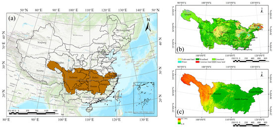
Figure 1.
General Map of the Study Area. (a) The location of the study area in China. (b) The land use and administrative division of the study area in 2020. (c) The topography of the study area and the distribution of its upper, middle, and lower reaches.
2.2. Data Sources and Preprocessing
The primary data required for this study included socioeconomic data, accessibility data, and natural environmental factors. The data sources are listed in Table 1. Due to inconsistencies in data types and spatial resolutions, all datasets were resampled (or rasterized) to a spatial resolution of 100 × 100 m prior to analysis and projected using the WGS_1984_UTM_Zone_48N coordinate system. Land use data were reclassified into six major categories based on the original classification scheme (cultivated land, grassland, woodland, water bodies, built-up land, and unused land). Other datasets underwent appropriate preprocessing according to the computational requirements of the model.

Table 1.
Key Data and Sources.
2.3. Research Methods
2.3.1. HQ Assessment Based on the InVEST Model
This study integrated the specific conditions of the research area, categorizing habitat types into four threatening factors (cultivated land, construction land, unused land, and roads). The maximum stress impact distance, relative weight, and spatial decay type of these threatening factors were determined. Using the HQ module in the InVEST software (V.3.13.0), the HQ of the study area was calculated [45]. The formula is as follows:
In the formula, j represents the habitat type, Qxj represents the HQ of grid cell x in land use and land cover type j, Dxj represents the stress level experienced by grid cell x in land use type j, k is the half-saturation constant, typically taken as half of the maximum value of Dxj, Hj is the habitat suitability of land use type j, and z is the normalization constant. Dxj is calculated using the following formula:
In the formula,
R is the threat factor,
y is the number of grid cells in the raster layer of threat factor r,
YR is the number of grid cells occupied by the threat factor,
Wr is the weight of threat factor r,
Ry is the value of the threat factor for grid cell y (0 or 1),
Irxy is the threat level imposed on habitat grid cell x by the threat factor value ry of grid cell y,
βx is the accessibility level of grid cell x, ranging from 0 to 1, where 1 indicates extremely easy access, and
Sjr is the sensitivity of habitat type j to threat factor r.
The value of irxy is determined using the following formula:
In the formula,
Dy is the Euclidean distance between grid cell x and grid cell y, and
Drmax is the maximum influence distance of threat factor r.
The data required to run the HQ module include land use and land cover maps for each period, threat factor layers for each period, the influence distances of threat factors, the sensitivity of habitats to each threat factor, and the distances between habitats and threat factor sources. The habitat suitability, relative sensitivity of threat sources, maximum stress distance, weights, and spatial decay types of each factor were determined by referring to the relevant literature and combining them with the specific conditions of the study area (Table 2 and Table 3) [46,47].
Table 2.
Habitat Suitability and Relative Sensitivity to Threat Sources.
Table 3.
Threat Sources, Weights, and Maximum Impact Distances.
2.3.2. HQ Coefficient of Variation
The CV is often used to measure the relative stability (or fluctuation) of geographic data over time [48,49] and was applied here to evaluate the stability of HQ in the YRB over the past 21 years. The calculation formula is as follows:
In the formula, CV is the coefficient of variation, HQ is the value for year i, n is the width of the time series, and is the average HQ in the YRB from 2000 to 2020. A larger CV indicates larger fluctuations in HQ over the time series, while a smaller CV indicates smaller fluctuations.
2.3.3. Theil–Sen Median Trend Analysis and the Mann–Kendall Test
Theil–Sen median trend analysis [50] and the Mann–Kendall test [51] are important methods for determining trends in long-term time series data [52]. These methods are particularly useful for assessing trends in data where the underlying distribution is unknown or not necessarily Gaussian. They were used to evaluate the trends in HQ in the YRB over the past 21 years. The calculation formulas are as follows:
where β is the change trend and HQi/j is the HQ value in year i/j. When β > 0, the HQ of the region showed an upward trend. When β < 0, the HQ of the region showed a downward trend.
The Mann–Kendall test was used to determine whether the changes in NPP trends in the region are statistically significant. The calculation formula is as follows:
where sgn is the sign function. Furthermore, the trend test was based on the null hypothesis H0: β = 0. The null hypothesis was rejected when |ZC| > Z1-a/2, where Z1-a/2 is the standard normal variance, α is the significance test level, and α < 0.05 passes the significance test when |ZC| ≥ 1.64, indicating a significant change in the region.
2.3.4. Future Trend Analysis
The Hurst index is used to quantitatively describe the long-term dependence of HQ time series information [53,54]. The basic principle is as follows. For a given HQ time series {HQ (τ)}, the mean value series is defined as follows for any positive integer:
X(t) represents the cumulative deviation:
The range R(τ) is defined as:
The standard deviation S(τ) is defined as:
If R/S∝τH, the Hurst phenomenon is present in the HQ time series, where H is the Hurst index obtained by least squares fitting. The value of H ranges from 0 to 1 and includes three scenarios:
- (1)
- If H > 0.5, the time series has persistence. The closer H is to 1, the stronger the persistence;
- (2)
- If H = 0.5, the time series is random;
- (3)
- If H < 0.5, the time series has anti-persistence. The closer H is to 0, the stronger the anti-persistence.
2.3.5. PLUS Model for Future Land Use Simulation
- (1)
- LEAS and Driving Factors.
To provide data support for studying the future HQ in the YRB, a Patch-Growth Land Use Simulation (PLUS) model was used to predict land use changes in the study area by 2030. This model integrates a rule-mining method based on land expansion analysis and a cellular automaton model with a multi-type random seed mechanism [55]. The land expansion analysis strategy uses rule mining to extract parts of land use changes related to the expansion of different land types. It employs a random forest algorithm to explore the relationships between each land use expansion and its contributing factors, obtaining the development probability of each land type and the weight of influencing factors from drivers [56]. The formula for calculating the rule-mining method based on land expansion analysis is as follows:
In the equation, represents the development probability of land use type K in cell i, d takes values of 0 or 1, where 1 denotes conversion from other land use types to K, and 0 denotes no conversion, I( ) is the function read by the random forest decision tree, hn denotes the nth decision tree classification model, and M represents the number of decision trees.
- (2)
- Future Simulation of CARS
The Cellular Automata Model with Multi-class Random Patch Seeds (CARS) is an advanced tool for land use simulation. This model divides the land into a series of small areas, each of which is called a cell. Each cell has a certain state that can be updated and evolved according to specific rules. By defining appropriate rules and algorithms, the model can simulate the dynamic changes in land use. The formula is as follows:
In the equations, represents the overall transition probability of cell unit i transitioning from its original land use type to land use type k at time t, denotes the neighborhood influence factor, signifies the adaptive inertia coefficient, R denotes a random number ranging from 0 to 1, and uk represents the generation threshold for land use type k, which is set by the user.
Furthermore, a threshold decrement mechanism was employed to control the generation of land use patches. When a new land use type prevails in competition, the decrement threshold affects the candidate land use types generated by roulette selection. The specific calculation formula is as follows:
In the equations, and respectively represent the difference between the number of grid cells of land type c at time t-1 and t and the corresponding demand quantities, Step denotes the increment step of the PLUS model toward meeting land use demands, (1) signifies the number of generations for the decrement step, represents the decay coefficient of decrement value , r1 denotes a random value following a normal distribution within the range [0, 2], and signifies the land use transition matrix determining whether land use type c transitions to type k.
This study established three scenarios based on natural growth for future land use projections:
- The natural development scenario (S1), which assumes that transition probabilities from 2020 to 2035 follow the natural growth trend observed from 2010 to 2020;
- The farmland protection scenario (S2), which reduces the probability of farmland converting to other land types by 50% compared with the natural development scenario, while other land types continue to follow natural development trends;
- The ecological conservation scenario (S3), which, compared with the natural development scenario, reduces the probability of farmland, forest land, grassland, and water bodies converting to built-up land by 30%, 50%, 20%, and 20%, respectively. Additionally, S3 reduces the probability of forest land converting to grassland by 50%, while increasing the probability of water bodies and grassland converting to forest land by 20%. The probability of built-up land converting to forest land is increased by 10%.
3. Results
3.1. Land Use Changes in the YRB
Between 2000 and 2020, the YRB maintained the land use type proportion order of “woodland > cultivated land > grassland > water > unused land > construction land”, with forest and cultivated land as the dominant types, collectively accounting for over 65%, though their shares declined. As shown in Table 4 and Figure 2, cultivated land had the largest area transferred out at 562,087.6 km2, with a net reduction of 23,211.28 km2. Most of this cultivated land was converted to construction land and woodland. Construction land showed the most significant increase, expanding by 86.96% and adding 25,230.24 km2, primarily sourced from cultivated land followed by woodland and grassland. Despite a large transfer-out area of 421,364.4 km2 for woodland, its total area increased by 98,333.2 km2, mainly converted from cultivated land and grassland. Other changes include a 16.00% reduction in unused land, a decrease in grassland by 5811.12 km2, and an increase in water bodies by 4932.64 km2.
Table 4.
Land Use Area and Proportional Changes in the YRB (2000–2020).
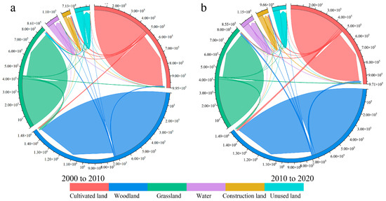
Figure 2.
String map of land use transfer between different types from 2000 to 2020: (a) from 2000 to 2010; (b) from 2010 to 2020.
In this study, the spatial distribution of construction land changes that significantly impacted HQ was analyzed. The results reveal that the areas where construction land increased in the study region can be categorized into three main types. The first type is attributed to urban expansion, characterized by incremental block-like expansion outward along the periphery of existing developed areas. This type of change was primarily concentrated in the Chengdu–Chongqing Economic Zone in the upper reaches of the YRB, the Wuhan Metropolitan Area in the middle reaches of the Yangtze River, and the Yangtze River Delta urban cluster in the lower reaches. The second type is driven by linear engineering projects such as roads (including railways), resulting in linear expansion. This type of change mainly occurred between urban clusters, with a higher concentration in the middle and lower reaches of the Yangtze River (see Figure 3). The third type is characterized by discrete patches and was primarily concentrated in peri-urban areas and rural regions. In contrast, the reduction in construction land did not exhibit any concentrated spatial patterns and was scattered in rural areas.
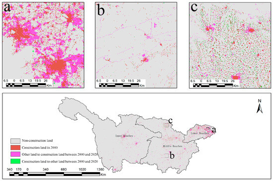
Figure 3.
The spectrum of changes between construction land and non-construction land in the YRB from 2000 to 2020 is as follows: (a) construction land in the form of patch expansion; (b) construction land in the form of linear expansion; (c) construction land in the form of discrete patches.
3.2. The Spatiotemporal Characteristics of HQ
3.2.1. HQ Assessment and CV
HQ is scored between 0 and 1, with lower values indicating worse quality. Using the InVEST-HQ model, the HQ in the YRB was calculated for 2000–2020, with the results shown in Figure 4. The annual HQ index averaged between 0.599 and 0.606 from 2000 to 2020, indicating relatively good HQ. Spatially, the quality was highest in central areas and lower in western plateaus and eastern plains, with low-quality clusters in areas like the Tibetan Plateau, Sichuan Basin, and Yangtze River estuary, especially near cities (dark red areas in Figure 3). The lowest quality was in eastern mountains and lakes. Over 21 years, the HQ ranked from lowest to highest as follows: lower Yangtze (0.478–0.515), upper Yangtze (0.589–0.593), and middle Yangtze (0.636–0.649). One-way ANOVA revealed that these differences were statistically significant (p < 0.05). As shown in Figure 4, the CV in the YRB was 0.350–2.720 (averaging 0.768), suggesting relatively stable HQ with some spatial variation. Areas with greater fluctuations in spatial distribution were classified into three types: fluctuations in urban fringe areas, such as the Yangtze River estuary and Chengdu Plain; linear fluctuation zones, mainly in the middle Yangtze region; and scattered distribution, mainly in mountainous regions such as the Kunlun Mountains.
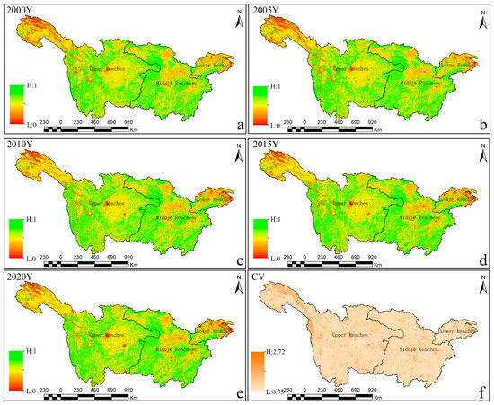
Figure 4.
Spatial distribution maps of HQ and stability in the YRB for selected years. (a–e) Spatial distribution maps of HQ in 2000, 2005, 2010, 2015, and 2020; (f) spatial distribution map of the grid-scale CV index.
3.2.2. Theil–Sen Median Trend Analysis and the Mann–Kendall Test
The β value of HQ in the YRB ranged from −0.295 to 0.291. The HQ remained unchanged across 76.98% of the basin’s area, decreased in 15.83% of the basin’s area, and increased in 7.18% of the basin’s area. Overall, there was a slight increasing trend, with an average β value of −0.001, indicating a weak decreasing trend. Areas with increasing trends were mainly concentrated on the Qinghai–Tibet Plateau and the Hengduan Mountains, while areas with decreasing trends were mainly around cities and along newly constructed roads (see Figure 5).
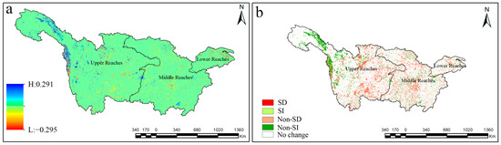
Figure 5.
Change trend map of HQ in the YRB. (a) Spatial distribution of grid-scale β index; (b) spatial distribution of Mann–Kendall test results for change trends.
By overlaying the results of the Theil–Sen median trend analysis and the Mann–Kendall test, four scenarios were identified: Significant Increase (SI), Significant Decrease (SD), Non-Significant Increase (Non-SI), and Non-Significant Decrease (Non-SD). The results show that approximately 77.51% of the YRB experienced no significant change in HQ over the past 21 years, which corroborates the previous finding of relatively stable regional HQ. Areas with decreasing trends accounted for 15.15% of the region, with SD areas making up 3.56% of the study area, primarily distributed in block-like patterns around cities and linearly along newly constructed high-grade roads. Non-SD areas accounted for 11.60% of the study area, mainly concentrated around SD areas and distributed in a layered pattern. Areas with increasing trends accounted for 7.33% of the region, concentrated on the Qinghai–Tibet Plateau and the Hengduan Mountains, with scattered point-like distributions in the middle and lower Yangtze River Plain. Among these, SI areas accounted for only 0.95% of the total area, sporadically distributed across the region, indicating a weak future growth trend, while Non-SI areas accounted for 6.38% of the total area.
3.3. Simulation Results of LUCC Under Multiple Scenarios in the YRB in 2030
In this study, Markov-chain-based predictions of 2020 land use demand, trained on 2000 and 2010 data and incorporating 13 YRB-specific driving factors in the PLUS model, were integrated with transition matrices and zonal weights in the CARS module to simulate 2020 land use. The simulation, validated against observed 2020 land use, showed high accuracy (Kappa = 0.891, Fom = 0.169).
The PLUS model generated spatial distribution maps for three YRB development scenarios (Figure 6). All scenarios showed consistent future functional zoning, with urbanization concentrated in the Yangtze River Delta, Wuhan Metropolitan Area, and Chengdu–Chongqing Economic Zone, but differing in land use quantities (Table 5).
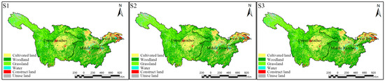
Figure 6.
Spatial Distribution Map of Land Use in the YRB under Three Different Development Scenarios.
Table 5.
Land Use Quantity Structure in the YRB under Three Different Development Scenarios. (Unit: km2).
In S1, cultivated land and woodland dominated, and grassland was relatively extensive, reflecting a market-driven balance between traditional agriculture and natural ecosystems. However, the construction land expansion and grassland reduction highlighted urbanization’s pressure on natural vegetation.
In S2, policy interventions increased cultivated land to 921,717.6 km2 but reduced forest by 1.1%, showing the trade-off between agricultural expansion and ecological land. Construction land contracted to 587,722.8 km2, indicating that intensive land use policies curbed disorderly construction land growth.
S3 prioritized ecosystems, with woodland increasing to 7,531,954.8 km2 (the highest among all scenarios) and cultivated land falling to 4,772,000.8 km2, near natural development levels, suggesting that quality improvements and spatial optimization replaced scale expansion. Grassland and construction land fluctuations eased, likely due to ecological restoration and planning controls.
3.4. Future Measurement of HQ
In this study, land use data from three development scenarios simulated by the PLUS model were input into the InVEST-HQ model to calculate the HQ for the YRB in 2030. The assessment of HQ evolution in the YRB under different development scenarios in 2020 and 2030 is presented in Table 6. The results show that the YRB HQ index exhibited a downward trend under all three scenarios, with significant differences in the degree of decline.
Table 6.
Comparison of HQ Mean Evaluation Results for the YRB in 2020 and 2030 Under Different Scenarios.
Under scenarios S1 and S2, the habitat quality (HQ) index of the Yellow River Basin (YRB) decreased by 1.07% (to 0.5927) and 1.15% (to 0.5922), respectively. In contrast, scenario S3, which incorporated development intensity restrictions and ecological restoration measures, effectively limited the decline to 0.33% (to 0.5971), demonstrating a significant capacity to mitigate habitat degradation. This mitigation can be attributed to targeted ecological protection strategies under S3, such as wetland restoration, enhanced forest conservation, and restrictions on land development, which played a key role in buffering against the negative ecological impacts of land use change.
Spatial differences in HQ change patterns were also evident across scenarios (Figure 7). In the northern Hengduan Mountains, where ecological sensitivity is high, both S1 and S3 showed clusters of HQ improvement, with S3 exhibiting a more pronounced spatial extent, highlighting the positive influence of ecological restoration policies. In contrast, in the middle reaches of the Yangtze River, areas experiencing an HQ decline were substantially larger under scenarios S1 and S2, while scenario S3 exhibited a visibly smaller degraded area, indicating that the ecological protection policies in S3 effectively curbed habitat degradation.
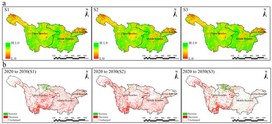
Figure 7.
(a) Spatial distribution of HQ in the YRB in 2030 under different scenarios. (b) Distribution map of changes in 2030 compared to 2020 under different scenarios.
Specifically, in the downstream section of the middle reaches, the HQ index under scenario S1 declined by 3.24% compared with 2020 (to 0.4627), with extensive areas undergoing degradation. While scenarios S2 (0.4727) and S3 (0.4755) alleviated the pressure to some extent through cropland protection and ecological regulation, they could not fully reverse the downward trend, underscoring the region’s ecological fragility and the limitations of partial interventions.
In the middle reaches overall, favorable natural conditions supported relatively high HQ levels across all scenarios, with minimal degradation observed, suggesting strong ecological resilience in this area. In the upper reaches, the continued development pressure under scenarios S1 and S2 led to HQ declines of 0.86% and 1.23%, respectively. However, under S3, the decline was narrowed to 0.46% (to 0.5869), representing a notable improvement over other scenarios and reflecting the effectiveness of integrated ecological protection policies in mitigating degradation.
4. Discussion
4.1. The Driving Mechanism of the Temporal Trend of HQ
The HQ in the YRB is projected to decline from 2000 to 2030, with no short-term reversal in sight. Although regional ecological protection policies have partially slowed habitat degradation, the combined effects of intense human activities and climate change will likely maintain the overall downward trend. The main drivers are as follows.
Land-use conversion driven by urbanization: Between 2000 and 2020, construction land in the YRB increased by 25,230 km2, primarily through the conversion of cropland and forest. This directly caused habitat fragmentation. Not only did the increase in construction land alter the local HQ, but it also created stress effects on the surrounding HQ. In particular, the “patch-like urbanization” and “linear road expansion” patterns of urban sprawl had the most significant dissecting effect on habitats (Figure 8). For example, the construction of the Wuhan Metropolitan Area led to a significant decline in the surrounding HQ. The expansion of road networks (e.g., highways, railways) further intensified this effect, creating a unique “corridor–patch” degradation pattern. The ongoing conversion of cropland and forest (which decreased by 23,211 km2 and 5811 km2, respectively) also compressed species’ habitats, consistent with the conclusion of studies on urban sprawl in North America that “edge expansion dominates habitat fragmentation” [57].
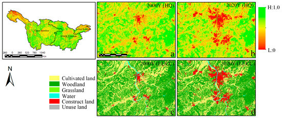
Figure 8.
Contrasting Patterns of HQ Variation and Land Use Change in Central China’s Urban Expansion Zones, (a) HQ in 2000; (b) HQ in 2020; (c) LUCC in 2000; (d) LUCC in 2020.
The trade-offs between agricultural expansion and ecological land use: In the S2 scenario, farmland protection policies restricted the conversion of farmland to construction land, curbing short-term construction land expansion. However, this policy led to a 1.1% decrease in forest land (from 734,671.6 km2 to 734,671.5 km2) as it became the main land type converted to meet land demands, resulting in the lowest HQ (0.5922) among the three scenarios (Figure 9). This highlights the structural conflict between agricultural expansion and ecological land use. From a driving mechanism perspective, farmland protection policies restricted land-use conversion through administrative means but did not improve farmland efficiency or promote intensive agricultural development. In the middle and lower Yangtze River regions, to ensure food security, some sloping forest lands were converted to farmland, weakening biodiversity functions. Additionally, the “leakage effect” during policy implementation exacerbated the conflict. To avoid farmland protection restrictions, some rural areas targeted forest land for development, indirectly converting it to farmland and then to construction land, achieving land development goals.
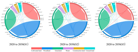
Figure 9.
String map of land transfer among land uses under different scenarios in the YRB from 2000 to 2030.
Climate responses and ecological vulnerability in the upper reaches: In the Qinghai–Tibet Plateau and Hengduan Mountain regions, warming (the average temperature increased from −4.44 °C in 2000 to −3.74 °C in 2020) caused the perennial snow cover to shift to higher altitudes, converting some land to grassland. This local ecological change improved the HQ (Figure 10), but it did not significantly benefit the overall HQ of the YRB and may trigger long-term ecological risks like accelerated permafrost thawing. This finding aligns with the IPCC (2021) theory of “land use–climate–biodiversity” coupling effects [58], highlighting that the stress from intense human activities on ecosystems has cumulative spatial and cross-scale transmission characteristics.
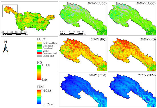
Figure 10.
Dynamics of Land Use and Land Cover (LUCC), HQ, and Temperature in Representative High-Altitude Regions (2020–2030).
4.2. Spatial Heterogeneity of HQ and Its Driving Mechanisms
As the region of China with the most complex ecological functions and the highest socioeconomic activity, the YRB shows distinct spatiotemporal differences in HQ that profoundly reflect the dynamic interplay between natural geographic gradients and the intensity of human activities. The spatial heterogeneity of HQ in the basin is not randomly distributed but shows significant geographic gradient effects, with a general pattern of “high in the middle reaches and low in the upper and lower reaches”. This heterogeneity is jointly shaped by multi-scale driving mechanisms, including the baseline effects of natural geographical conditions, the spatially differentiated stress of human activities, the differentiated impacts of climate change on ecosystems at different elevation gradients, and the significant differences in development models and ecological responses between urban and rural areas.
The YRB, spanning China’s three major topographic steps with complex and diverse landforms, shows distinct spatial heterogeneity in HQ, shaped by natural and human factors. In the middle reaches (e.g., Jianghan Plain and Dongting Lake Basin), flat terrain, abundant precipitation, and dense water networks have formed wetland and evergreen broad-leaved forest ecosystems. For example, in 2020, forests accounted for 54.13% of land cover in the middle reaches, markedly higher than in the upper (21.89%) and lower reaches (34.46%). Correspondingly, the HQ index in the middle reaches (0.636–0.649) was significantly higher than in the upper (0.589–0.593) and lower (0.478–0.515) reaches. These natural conditions support biodiversity and buffer against human-induced disturbances through ecosystem self-organization processes like wetland regulation and forest carbon sinks. In contrast, the lower Yangtze Delta, with its flat terrain and farmland-dominated land use, is a key urbanized area in China. Its weaker resistance to ecosystem disturbances makes the HQ more vulnerable to construction land expansion. The Qinghai–Tibet Plateau in the upper reaches, though ecologically fragile, has maintained relatively stable HQ over two decades due to its high elevation, its low population density (<10 people/km2) [59], and the implementation of strict ecological conservation policies, such as the establishment of the Sanjiangyuan National Nature Reserve and the Hoh Xil Nature Reserve.
4.3. Synergistic Pathways of Cross-Scale Governance and Ecological Resilience Enhancement
The degradation and spatial heterogeneity of HQ in the YRB call for a multi-scale governance framework that aligns natural geographic foundations, human development intensity, and climate adaptation strategies. In the highly urbanized lower reaches, where habitat fragmentation is pronounced, a dual strategy of “rigid regulation” and “flexible restoration” should be employed to rebuild ecological connectivity. For instance, in the Yangtze River Delta, ecological protection red lines should be refined based on existing ecological sensitivity assessments and land-use conflict analyses. Priority ecological corridors—such as migratory bird flyways along coastal wetlands and major fish spawning routes linked to tributaries—should be identified using habitat suitability modeling and protected through zoning and green infrastructure planning. Additionally, promoting vertical greening and rooftop ecological systems in high-density urban areas offers a feasible pathway to enhancing local biodiversity without competing for land.
In the middle reaches, where agricultural production is dominant, governance should transition from merely protecting agricultural quantity to improving ecological quality. This can be achieved through the promotion of ecological farming techniques such as reduced pesticide use, intercropping with native species, and wetland-buffered rice paddies. Supporting these models with incentive-based mechanisms (e.g., agri-environmental subsidies) can improve both land productivity and ecological resilience.
In the ecologically fragile upper reaches, climate adaptation and the optimization of protected area networks are essential. Establishing climate monitoring stations in the permafrost regions of the Qinghai–Tibet Plateau may enhance early warning systems for ecosystem changes. Moreover, connecting existing protected areas via planned ecological corridors—guided by species distribution patterns and topographic connectivity—can facilitate wildlife migration and promote long-term genetic exchange.
The success of cross-scale governance depends on institutional integration and stakeholder coordination. Current fragmented administrative systems often generate conflicts, such as downstream development pressures conflicting with upstream conservation. Therefore, an inter-provincial horizontal ecological compensation mechanism—coordinated by basin-level ecological governance platforms—should be established to redistribute development costs and conservation benefits. This regionally tailored and process-integrated governance pathway provides a systematic framework for enhancing ecological resilience and advancing sustainable development in the YRB.
4.4. Research Limitations and Future Research
This study has several limitations related to model accuracy, data resolution, and the depth of the driving mechanism analysis. First, the InVEST and PLUS models have inherent constraints in simulating the complex processes of land use and ecosystem dynamics. Specifically, the threat factor weights used in the InVEST model have not undergone sufficient local validation, which may result in under- or overestimation of the relative importance of key threats, thereby affecting the accuracy and reliability of habitat quality assessments. Future work should focus on calibrating these weights through field surveys and expert elicitation, incorporating local ecological characteristics, and conducting sensitivity analyses to improve the model’s applicability and regional representativeness. Second, the current scenario simulations exclude extreme climate events (e.g., floods, droughts) and abrupt policy changes (e.g., significant environmental regulations), potentially underestimating dynamic ecosystem responses and limiting the scientific robustness of future projections.
To overcome these limitations, future research should integrate high-resolution remote sensing data with ground-based monitoring to improve the spatial and temporal precision of model inputs, thereby enhancing the accuracy and credibility of simulation outputs. Moreover, designing diverse policy scenarios—such as carbon neutrality goals and ecological compensation mechanisms—would better reflect prospective policy environments, increasing the foresight and practical relevance of ecological protection strategies. Finally, fostering interdisciplinary collaboration and stakeholder engagement is crucial for translating scientific findings into actionable management practices, ultimately promoting the sustainable development of large-scale river basins.
5. Conclusions
Based on the tripartite analysis framework of “remote-sensing big data–socioeconomic data–ecological models” and by integrating the InVEST and PLUS models, this study systematically evaluated the spatiotemporal evolution of HQ in the YRB from 2000 to 2020. It also predicted HQ trends under three scenarios (natural development, farmland protection, and ecological protection) for 2030. The findings are as follows:
- Spatiotemporal HQ characteristics: The YRB’s average HQ remained stable at 0.599–0.606 during 2000–2020, but the degree of spatial heterogeneity was significant, with a “high in the middle reaches and low in the upper and lower reaches” pattern. The lower reaches had the lowest HQ due to urbanization-related ecological fragmentation. Trend analysis showed that while 76.98% of the area saw no significant HQ change, 15.83% of the area saw a decline, with 3.56% experiencing significant degradation, mainly in construction land expansion areas;
- Future scenario simulation: Under all three 2030 scenarios, the YRB’s HQ is expected to decline. However, S3 limited the decline to 0.33% through controlled development and ecological restoration, outperforming natural development (a 1.07% decline) and farmland protection (a 1.15% decline). The lower reaches will remain ecologically vulnerable and face high-risk degradation even under S3;
- Habitat degradation was primarily driven by urban expansion, cropland encroachment, and climate-induced land cover shifts. The emergence of a “corridor–patch” fragmentation pattern—associated with linear infrastructure and peri-urban sprawl—underscored the spatial complexity of human-induced habitat stress. Moreover, trade-offs between farmland protection and forest loss revealed unintended ecological consequences of sectoral policies;
- The results provide evidence-based support for differentiated policy interventions across the YRB. Recommendations include zoning-based ecological red lines and green infrastructure in urbanized lower reaches, eco-agriculture and incentive mechanisms in the middle reaches, and climate-adaptive conservation networks in the upper plateau. Establishing cross-regional ecological compensation mechanisms is essential to reconcile upstream protection with downstream development.
Author Contributions
Y.Z.: conceptualization, data curation, formal analysis, writing—original draft, writing—review and editing; J.Y.: project administration, software, supervision, validation, formal analysis, writing—review and editing; W.W.: investigation and visualization; D.T.: conceptualization and methodology. All authors have read and agreed to the published version of the manuscript.
Funding
This work was supported by the National Natural Science Foundation of China (NO.42101275); and the Provincial Natural Science Foundation of Hubei, China (NO. 2023AFB651).
Institutional Review Board Statement
Not applicable.
Informed Consent Statement
Not applicable.
Data Availability Statement
The data presented in this study are available upon request from the corresponding author. The data are not publicly available due to privacy restrictions.
Acknowledgments
The authors are grateful to the editor and reviewers for their valuable comments and suggestions.
Conflicts of Interest
The authors declare no conflicts of interest.
Abbreviations
The following abbreviations are used in this manuscript:
| YRB | Yangtze River Basin |
| HQ | Habitat quality |
| PLUS | Patch-Growth Land Use Simulation |
| RS | Remote sensing |
| GIS | Geographic information system |
| InVEST | Integrated Valuation of Ecosystem Services and Trade-offs |
| LUCC | land use/cover change |
References
- Gong, J.; Cao, E.; Xie, Y.; Xu, C.; Li, H.; Yan, L. Integrating ecosystem services and landscape ecological risk into adaptive management: Insights from a western mountain-basin area, China. J. Environ. Manag. 2021, 281, 111817. [Google Scholar] [CrossRef] [PubMed]
- Wang, S.; Wu, M.; Hu, M.; Xia, B. Integrating ecosystem services and landscape connectivity into the optimization of ecological security pattern: A case study of the Pearl River Delta, China. Environ. Sci. Pollut. Res. Int. 2022, 29, 76051–76065. [Google Scholar] [CrossRef]
- Vicente-Serrano, S.M.; Pricope, N.G.; Toreti, A.; Morán-Tejeda, E.; Spinoni, J.; Ocampo-Melgar, A.; Archer, E.; Diedhiou, A.; Mesbahzadeh, T.; Ravindranath, N.H.; et al. The United Nations Convention to Combat Desertification Report on Rising Aridity Trends Globally and Associated Biological and Agricultural Implications. Glob. Change Biol. 2024, 30, e70009. [Google Scholar] [CrossRef]
- Eigenbrod, F.; Bell, V.A.; Davies, H.N.; Heinemeyer, A.; Armsworth, P.R.; Gaston, K.J. The impact of projected increases in urbanization on ecosystem services. Proc. R. Soc. B Biol. Sci. 2011, 278, 3201–3208. [Google Scholar] [CrossRef]
- Fang, C.; Wang, J. A Theoretical Analysis of Interactive Coercing Effects Between Urbanization and Eco-environment. Chin. Geogr. Sci. 2013, 23, 147–162. [Google Scholar] [CrossRef]
- Liu, Y.; Yao, C.; Wang, G.; Bao, S. An integrated sustainable development approach to modeling the eco-environmental effects from urbanization. Ecol. Indic. 2011, 11, 1599–1608. [Google Scholar] [CrossRef]
- Elliott, R.J.; Shanshan, W.U. Industrial activity and the environment in China: An industry-level analysis. China Econ. Rev. 2008, 19, 393–408. [Google Scholar]
- Gavrilov, O.E.; Eremeeva, S.S.; Karaganova, N.G.; Kazakov, A.V.; A Mironov, A. Ecological activity area formation of an industrial enterprise: Applied aspects. IOP conference series. Earth Environ. Sci. 2021, 677, 52059. [Google Scholar]
- Wang, Y. Environmental degradation and environmental threats in China. Environ. Monit. Assess. 2004, 90, 161. [Google Scholar] [CrossRef]
- Pacheco, F.A.L.; Fernandes, L.F.S.; Junior, R.F.V.; Valera, C.A.; Pissarra, T.C.T. Land degradation: Multiple environmental consequences and routes to neutrality. Curr. Opin. Environ. Sci. Health 2018, 5, 79–86. [Google Scholar] [CrossRef]
- Intergovernmental Panel on Climate Change. Convention on Biological Diversity; Intergovernmental Panel on Climate Change: Geneva, Switzerland, 1992. [Google Scholar]
- Allen, C.; Metternicht, G.; Wiedmann, T. Initial progress in implementing the Sustainable Development Goals (SDGs): A review of evidence from countries. Sustain. Sci. 2018, 13, 1453–1467. [Google Scholar] [CrossRef]
- Hák, T.; Janoušková, S.; Moldan, B. Sustainable Development Goals: A need for relevant indicators. Ecol. Indic. 2016, 60, 565–573. [Google Scholar] [CrossRef]
- Diaz, R.J.; Solan, M.; Valente, R.M. A review of approaches for classifying benthic habitats and evaluating habitat quality. J. Environ. Manag. 2004, 73, 165–181. [Google Scholar] [CrossRef]
- Mortelliti, A.; Amori, G.; Boitani, L. The role of habitat quality in fragmented landscapes: A conceptual overview and prospectus for future research. Oecologia 2010, 163, 535–547. [Google Scholar] [CrossRef]
- Johnson, M.D. Measuring Habitat Quality: A Review. Condor 2007, 109, 489–504. [Google Scholar] [CrossRef]
- Riedler, B.; Lang, S. A spatially explicit patch model of habitat quality, integrating spatio-structural indicators. Ecol. Indic. 2018, 94, 128–141. [Google Scholar] [CrossRef]
- Kneib, T.; Müller, J.; Hothorn, T. Spatial smoothing techniques for the assessment of habitat suitability. Environ. Ecol. Stat. 2008, 15, 343–364. [Google Scholar] [CrossRef]
- Spanhove, T.; Borre, J.V.; Delalieux, S.; Haest, B.; Paelinckx, D. Can remote sensing estimate fine-scale quality indicators of natural habitats? Ecol. Indic. 2012, 18, 403–412. [Google Scholar] [CrossRef]
- Romero-Calcerrada, R.; Luque, S. Habitat quality assessment using Weights-of-Evidence based GIS modelling: The case of Picoides tridactylus as species indicator of the biodiversity value of the Finnish forest. Ecol. Model. 2006, 196, 62–76. [Google Scholar] [CrossRef]
- Zlinszky, A.; Heilmeier, H.; Balzter, H.; Czúcz, B.; Pfeifer, N. Remote Sensing and GIS for Habitat Quality Monitoring: New Approaches and Future Research. Remote Sens. 2015, 7, 7987–7994. [Google Scholar] [CrossRef]
- Henrys, P.A.; Jarvis, S.G. Integration of ground survey and remote sensing derived data: Producing robust indicators of habitat extent and condition. Ecol. Evol. 2019, 9, 8104–8112. [Google Scholar] [CrossRef] [PubMed]
- Wang, B.; Cheng, W. Effects of Land Use/Cover on Regional Habitat Quality under Different Geomorphic Types Based on InVEST Model. Remote Sens. 2022, 14, 1279. [Google Scholar] [CrossRef]
- Nematollahi, S.; Fakheran, S.; Kienast, F.; Jafari, A. Application of InVEST habitat quality module in spatially vulnerability assessment of natural habitats (case study: Chaharmahal and Bakhtiari province, Iran). Environ. Monit. Assess. 2020, 192, 487. [Google Scholar] [CrossRef]
- Mondal, I.; Naskar, P.K.; Alsulamy, S.; Jose, F.; Hossain, S.A.; Mohammad, L.; De, T.K.; Khedher, K.M.; Salem, M.A.; Benzougagh, B.; et al. Habitat quality and degradation change analysis for the Sundarbans mangrove forest using invest habitat quality model and machine learning. Environ. Dev. Sustain. 2024. [Google Scholar] [CrossRef]
- Piri Sahragard, H.; Ajorlo, M.; Karami, P. Modeling habitat suitability of range plant species using random forest method in arid mountainous rangelands. J. Mt. Sci. 2018, 15, 2159–2171. [Google Scholar] [CrossRef]
- Wang, H.; Bai, X.; Zhou, M.; Ma, Y.; Yuan, W.; Guo, W. Response to hydrometeorological changes and evaluation of habitat quality in the Dongting Lake basin, China. J. Water Clim. Change 2024, 15, 4536–4560. [Google Scholar] [CrossRef]
- Wang, J.; Wu, Y.; Gou, A. Habitat quality evolution characteristics and multi-scenario prediction in Shenzhen based on PLUS and InVEST models. Front. Environ. Sci. 2023, 11, 1146347. [Google Scholar] [CrossRef]
- He, J.; Huang, J.; Li, C. The evaluation for the impact of land use change on habitat quality: A joint contribution of cellular automata scenario simulation and habitat quality assessment model. Ecol. Model. 2017, 366, 58–67. [Google Scholar] [CrossRef]
- Slagter, B.; Tsendbazar, N.-E.; Vollrath, A.; Reiche, J. Mapping wetland characteristics using temporally dense Sentinel-1 and Sentinel-2 data: A case study in the St. Lucia wetlands, South Africa. Int. J. Appl. Earth Obs. Geoinf. 2020, 86, 102009. [Google Scholar] [CrossRef]
- Seabrook, L.; McAlpine, C.; Rhodes, J.; Baxter, G.; Bradley, A.; Lunney, D. Determining range edges: Habitat quality, climate or climate extremes? Divers. Distrib. 2014, 20, 95–106. [Google Scholar] [CrossRef]
- Hu, Y.; Xu, E.; Dong, N.; Tian, G.; Kim, G.; Song, P.; Ge, S.; Liu, S. Driving Mechanism of Habitat Quality at Different Grid-Scales in a Metropolitan City. Forests 2022, 13, 248. [Google Scholar] [CrossRef]
- Jiang, Y.; He, J.; Zhai, D.; Hu, C.; Yu, L. Analysis of the evolution of watershed habitat quality and its drivers under the influence of the human footprint. Front. Environ. Sci. 2024, 12, 1431295. [Google Scholar] [CrossRef]
- Chen, S.; Liu, X. Spatio-temporal variations of habitat quality and its driving factors in the Yangtze River Delta region of China. Glob. Ecol. Conserv. 2024, 52, e02978. [Google Scholar] [CrossRef]
- Nabikandi, B.V.; Rastkhadiv, A.; Feizizadeh, B.; Gharibi, S.; Gomes, E. A scenario-based framework for evaluating the effectiveness of nature-based solutions in enhancing habitat quality. GeoJournal 2025, 90, 55. [Google Scholar] [CrossRef]
- Struecker, B.; Milanovich, J. Predicted Suitable Habitat Declines for Midwestern United States Amphibians Under Future Climate and Land-Use Change Scenarios. Herpetol. Conserv. Biol. 2017, 12, 635–654. [Google Scholar]
- Shi, L.; Moser, S. Transformative climate adaptation in the United States: Trends and prospects. Science 2021, 372, eabc8054. [Google Scholar] [CrossRef]
- Yang, H.; Zhong, X.; Deng, S.; Xu, H. Assessment of the impact of LUCC on NPP and its influencing factors in the Yangtze River basin, China. Catena 2021, 206, 105542. [Google Scholar] [CrossRef]
- Wu, X.; Shen, Z.; Liu, R.; Ding, X. Land Use/Cover Dynamics in Response to Changes in Environmental and Socio-Political Forces in the Upper Reaches of Yangtze River, China. Sensors 2008, 8, 8104–8122. [Google Scholar] [CrossRef]
- Yang, H.; Zhong, X.; Deng, S.; Nie, S. Impact of LUCC on landscape pattern in the Yangtze River Basin during 2001–2019. Ecol. Inform. 2022, 69, 101631. [Google Scholar] [CrossRef]
- Yang, H.; Zhou, H.; Deng, S.; Zhou, X.; Nie, S. Spatiotemporal Variation of Ecosystem Services Value and its Response to Land Use Change in the Yangtze River Basin, China. Int. J. Environ. Res. 2024, 18, 17. [Google Scholar] [CrossRef]
- Jia, L.; Yu, K.; Li, Z.; Li, P.; Cong, P.; Li, B. Spatiotemporal pattern of landscape ecological risk in the Yangtze River Basin and its influence on NPP. Front. For. Glob. Change 2024, 6, 1335116. [Google Scholar] [CrossRef]
- Yang, X.; Meng, F.; Fu, P.; Zhang, Y.; Liu, Y. Spatiotemporal change and driving factors of the Eco-Environment quality in the Yangtze River Basin from 2001 to 2019. Ecol. Indic. 2021, 131, 108214. [Google Scholar] [CrossRef]
- Yangtze River Water Resources Commission, Ministry of Water Resources, Yangtze River Basin. 2024. Available online: https://www.britannica.com/place/Yangtze-River (accessed on 1 January 2025).
- Sallustio, L.; De Toni, A.; Strollo, A.; Di Febbraro, M.; Gissi, E.; Casella, L.; Geneletti, D.; Munafò, M.; Vizzarri, M.; Marchetti, M. Assessing habitat quality in relation to the spatial distribution of protected areas in Italy. J. Environ. Manag. 2017, 201, 129–137. [Google Scholar] [CrossRef]
- Zhu, Y.; Jia, P.; Liu, Y. Spatiotemporal evolution effects of habitat quality with the conservation policies in the Upper Yangtze River, China. Sci. Rep. 2025, 15, 5972. [Google Scholar] [CrossRef]
- Yang, F.; Yang, L.; Fang, Q.; Yao, X. Impact of landscape pattern on habitat quality in the Yangtze River Economic Belt from 2000 to 2030. Ecol. Indic. 2024, 166, 112480. [Google Scholar] [CrossRef]
- Alharbi, S.; Raun, W.R.; Arnall, D.B.; Zhang, H. Prediction of maize (Zea mays L.) population using normalized-difference vegetative index (NDVI) and coefficient of variation (CV). J. Plant Nutr. 2019, 42, 673–679. [Google Scholar] [CrossRef]
- Gallardo, A. Spatial Variability of Soil Properties in a Floodplain Forest in Northwest Spain. Ecosystems 2003, 6, 564–576. [Google Scholar] [CrossRef]
- Diop, L.; Bodian, A.; Diallo, D. Spatiotemporal Trend Analysis of the Mean Annual Rainfall in Senegal. Eur. Sci. J. 2016, 12, 231. [Google Scholar] [CrossRef]
- Amwata, D.A.; Muia, V.K.; Opere, A.O.; Ndunda, E. Rainfall and Temperature Trend Analysis using Mann-Kendall and Sen’s Slope Estimator Test in Makueni County, Kenya. J. Mater. Environ. Sci. 2024, 15, 349–367. [Google Scholar]
- Neeti, N.; Eastman, J.R. A Contextual Mann-Kendall Approach for the Assessment of Trend Significance in Image Time Series. Trans. GIS 2011, 15, 599–611. [Google Scholar] [CrossRef]
- Chronopoulou, A.; Viens, F.G. Hurst Index Estimation for Self-Similar Processes with Long-Memory. In Hurst Index Estimation for Self-Similar Processes with Long-Memory; Duan, J., Luo, S., Wang, C., Duan, J., Luo, S., Wang, C., Eds.; World Scientific: Singapore, 2010; pp. 91–117. [Google Scholar]
- Rehman, S. Study of Saudi Arabian climatic conditions using Hurst exponent and climatic predictability index. Chaos Solitons Fractals 2009, 39, 499–509. [Google Scholar] [CrossRef]
- Liang, X.; Guan, Q.; Clarke, K.C.; Liu, S.; Wang, B.; Yao, Y. Understanding the drivers of sustainable land expansion using a patch-generating land use simulation (PLUS) model: A case study in Wuhan, China. Comput. Environ. Urban Syst. 2021, 85, 101569. [Google Scholar] [CrossRef]
- Zhang, S.; Zhong, Q.; Cheng, D.; Xu, C.; Chang, Y.; Lin, Y.; Li, B. Landscape ecological risk projection based on the PLUS model under the localized shared socioeconomic pathways in the Fujian Delta region. Ecol. Indic. 2022, 136, 108642. [Google Scholar] [CrossRef]
- Haddad, N.M.; Brudvig, L.A.; Clobert, J.; Davies, K.F.; Gonzalez, A.; Holt, R.D.; Lovejoy, T.E.; Sexton, J.O.; Austin, M.P.; Collins, C.D.; et al. Habitat fragmentation and its lasting impact on Earth’s ecosystems. Sci. Adv. 2015, 1, e1500052. [Google Scholar] [CrossRef]
- Intergovernmental Panel on Climate Change. Climate Change 2021—The Physical Science Basis; IPCC: Geneva, Switzerland, 2023. [Google Scholar]
- Chen, H.; Yang, Q.; Su, K.; Zhang, H.; Lu, D.; Xiang, H.; Zhou, L. Identification and Optimization of Production-Living-Ecological Space in an Ecological Foundation Area in the Upper Reaches of the Yangtze River: A Case Study of Jiangjin District of Chongqing, China. Land 2021, 10, 863. [Google Scholar] [CrossRef]
Disclaimer/Publisher’s Note: The statements, opinions and data contained in all publications are solely those of the individual author(s) and contributor(s) and not of MDPI and/or the editor(s). MDPI and/or the editor(s) disclaim responsibility for any injury to people or property resulting from any ideas, methods, instructions or products referred to in the content. |
© 2025 by the authors. Licensee MDPI, Basel, Switzerland. This article is an open access article distributed under the terms and conditions of the Creative Commons Attribution (CC BY) license (https://creativecommons.org/licenses/by/4.0/).