Carbon Emission Prediction of the Transportation Industry in Jiangsu Province Based on the WOA-SVM Model

Abstract

The global environment has been facing sustainability threats recently owing to industrial and economic expansion. Hence, achieving the goals of carbon peak and carbon neutrality is crucial for promoting sustainable economic growth. To help the transportation industry achieve these goals, this study selects eight variables, including population size, per capita GDP, personal vehicle ownership, passenger and freight turnover, and green space coverage, as factors influencing the carbon emissions of the transportation industry in Jiangsu Province. This research uses these variables as the basis for predicting and analyzing transportation carbon emission trends from 2000 to 2021. In addition, the current study forecasts the future carbon emissions of the transportation industry and estimates the time of carbon emission peak in Jiangsu Province. To verify the accuracy of the results, this study compares the predicted results with those from other models. The whale optimization algorithm–support vector machine model is found to have the fewest errors among several models. On this basis, targeted measures are proposed to accelerate the carbon peak process and ensure the smooth achievement of carbon neutrality goals in Jiangsu Province. Results indicate that under the current policy measures, peak carbon emissions in Jiangsu Province will occur in 2038, with a peak of 48.72 million tons. Jiangsu Province should actively adopt energy-saving and emission-reduction measures, build a green and low-carbon transportation development model, and achieve the carbon peak target ahead of schedule. Findings from this study will provide valuable insights and practical recommendations for policy makers and stakeholders to formulate effective strategies for carbon reduction in the transportation sector, contributing to the sustainable development of China and the world.

1. Introduction

Global warming is a major challenge currently facing humanity [1], and a global consensus has indicated that the increase in the concentration of greenhouse gases, represented by carbon dioxide, is the main cause of climate warming. Accordingly, all countries have implemented energy-saving and emission-reduction measures to cope with this common challenge. With China’s carbon emissions surpassing those of the US in 2006, the former became the country with the largest carbon emissions for 14 consecutive years. China’s carbon emissions are significantly ahead of the US’, which is the second largest in the world [2]. As China is considered the leader of developing countries, reducing this country’s carbon emissions is important for promoting the sustainable growth of the domestic economy and is an important initiative to cope with global climate change. For this reason, the Chinese government has proposed the “dual carbon” goal to achieve carbon peak before 2030 and carbon neutrality before 2060.

Due to the aforementioned background, research related to carbon emissions has become a popular topic. Numerous scholars have conducted research from multiple perspectives, and novel research findings continue to emerge: Examining how contractual mechanisms coordinate sustainable supply chains under carbon emission goals and market uncertainty [3]. Evaluating the economic and environmental impact of carbon tax and carbon trading policies in a single-vendor single-buyer inventory model [4]. Examining the impact of China’s new urbanization policy on urban carbon emissions [5]. Studying how to optimize urban transport solutions for enhanced energy efficiency and reduced carbon emissions. [6]. Predicting carbon emissions and assessing carbon reduction policies [7]. Numerous studies show that multidimensional driver analysis and robust emission forecasting have consistently remained focal research areas in decarbonization studies [8,9,10].

Transportation has become one of the major carbon emission sectors in China, currently ranking as the third-largest source of carbon emissions in the country [11]. This sector, which accounts for 9% to 10% of the country’s total carbon emissions annually, has shown a year-on-year increase in emission proportions and has been identified as a key priority for decarbonization efforts. Meanwhile, reducing carbon emissions has also been identified as a key objective in the development of low-carbon transportation. In the research on driving factors of carbon emissions, scholars have utilized such methods as spatial correlation analysis [12], the logarithmic mean Divisia index (LMDI) method [13], and the stochastic impacts by regression on population, affluence, and technology (STIRPAT) model [14] to investigate energy intensity [15], energy structure, production input, output structure [16], and population [17], among others. These factors play dominant roles in carbon emissions in the transportation industry. Fan [18] classified the influence of related factors into positive drivers, negative drivers, and general constituents according to the contribution rate of carbon emissions. For the research on carbon peak prediction, most scholars have mainly relied on the establishment of prediction models to predict the time of carbon peak and portray the path of carbon peak. Moreover, the methods commonly used by academics for carbon emission prediction mainly include the gray prediction, STIRPAT, system dynamics, and time series models. Chai et al. [19], Yin [20], and Wang et al. [14] used the STIRPAT, gray prediction, and system dynamics models, respectively, to forecast carbon emissions. Among the time series models, the most commonly used is the autoregressive integrated moving average (ARIMA) model [21].

With the vigorous development of machine learning technology, numerous new algorithms have emerged, among which the support vector machine (SVM) stands out and demonstrates significant advantages. SVM has achieved increasing usage in the engineering, environment, and computing disciplines [22,23,24]. SVM, as an algorithm suitable for learning small sample data, is highly compatible with the characteristics of small sample datasets commonly used in the field of carbon emissions. At present, the SVM model has also been gradually applied to carbon emission prediction [25,26]. Given that the prediction accuracy of an SVM model generally depends on the proper selection of its parameters, the model must be optimized to achieve better performance compared with other models. Moreover, its strong robustness is particularly critical. This model needs to effectively deal with individual-year data anomalies caused by external factors, such as policy adjustments and economic fluctuations, thereby ensuring the stability and accuracy of predictions.

The existing literature indicates that predictive analyses on SVM models incorporating whale optimization algorithm (WOA-SVM) representations exhibit excellent performance in the engineering and agriculture fields. Zhou et al. [27] found that the optimized WOA-SVM is the best model among all proposed models in classifying tunnel squeezing and has the highest accuracy compared with other unoptimized individual classifiers (e.g., SVM, ANN, and GP). Zhou [28] compared the WOA-SVM model with SVM, decision tree (DT), k-nearest neighbors (KNN), and the SVM combined with the loop optimization algorithm (LOA-SVM) model. He proved that WOA-SVM has a high prediction accuracy, and that the analysis speed is fast and has good repeatability. Zhou et al. [29] evaluated the performance of SVM and its hybrid models (i.e., PSO-SVM, WOA-SVM) for daily ET₀ estimation across China’s diverse climatic zones and found that the WOA-SVM model outperforms others with superior accuracy and efficiency. However, this method has not yet been applied in the field of carbon emission prediction.

Therefore, this study applies the WOA-SVM method to carbon emission prediction. In particular, the current study constructs the WOA-SVM model and analyzes its accuracy and applicability. The model, combined with scenario analysis, predicts carbon emission trends in Jiangsu Province’s transportation sector under low-carbon, standard, and high-carbon scenarios. This study aims to explore a high-precision prediction method and to provide methodological guidance and data support for advancing carbon measurement and reduction efforts in the transportation sector.

The innovative aspects and main contributions of this study are primarily reflected in the following dimensions. First, in the parameter optimization of SVM, this research abandons the traditional grid search method and pioneers the application of WOA to transportation carbon emission forecasting. This algorithm integrates the breadth of global search with the precision of local search, thereby significantly reducing the risk of converging to the local optima. Second, this research conducts comprehensive performance evaluations and compares WOA-SVM with the unoptimized SVM model, k-nearest neighbors (KNN), Gaussian process regression (GPR), and WOA-SVM models, thereby providing additional intuitive demonstrations of model reliability. Lastly, the current study provides predictions of carbon emission peak times under different scenarios, offering recommendations and references for Jiangsu Province’s transportation sector to achieve its carbon peaking and carbon neutrality goals.

2. Materials and Methods

2.1. Selection of Indicators

The stochastic impacts by regression on population, affluence, and technology (STIRPAT) model is expanded from the impact–population–affluence–technology (IPAT) model [30] to study the impact of factors on environmental loads by quantitative analysis. Multiple independent variables related to scale, structure, and technology can be introduced into the model. In using the STIRPAT model to study carbon emissions, other factors that may impact such emissions can be introduced based on the actual situation of the study area. The related equation is shown as follows [31]:

$$I=a\times P^b\times B^c\times T^d\times e,$$

(1)

where $a$ is the constant term; $b,c,d$ are the exponential terms for P, B, and T, respectively; e is the error term; and $I,P,B,T$ represent the environment, population, economy, and technology, respectively.

The literature has indicated that carbon emissions from transportation are affected by population, economy, technology, and transportation [32]. Zhu [33] studied the influence of population size, economic growth, and energy intensity on transportation carbon emissions. Xu [34] selected and analyzed economic growth, urbanization rate, number of private cars, cargo turnover, and energy efficiency as key factors affecting the carbon emissions of the transportation sector. Xu X [12] believed that transportation intensity, urbanization level, technology level, per capita GDP, and industrial structure have direct roles in carbon emissions. Therefore, this study used the STIRPAT model and results of existing studies on the factors affecting carbon emissions as the bases, combined with the availability of data, for selecting eight variables from the four dimensions of population, economy, technology, and transportation as the main factors affecting carbon emissions in Jiangsu Province’s transportation industry: total population, per capita GDP, motor vehicle ownership, passenger turnover, cargo turnover, urbanization rate, urban green space coverage, and carbon emission intensity. In particular, carbon emission intensity refers to the transportation carbon emissions brought on by growth in unit GDP.

2.2. Transportation Carbon Emissions Measurement

This study adopts the “top-down” carbon emission calculation method in the IPCC 2006 Guidelines for National Greenhouse Gas Inventories [35] to calculate carbon emissions from transportation based on transportation fuel consumption combined with input–output analysis and carbon emission factor accounting methods. The corresponding calculation formulas are as follows [36]:

$$C={\displaystyle \sum _i{C}_i}={\displaystyle \sum _i{E}_i\times F_i}={\displaystyle \sum _i{E}_i\times {ALV}_i}\times {CV}_i\times {COF}_i\times {\displaystyle \frac{44}{12}},$$

(2)

where $i$ is the type of energy, which is divided into raw coal, gasoline, diesel, electricity, natural gas, fuel oil, and liquefied petroleum gas; $Ei$ is the consumption of energy type; $Fi$ is the carbon emission coefficient of the energy; $ALVi$ is the average status of heat generation; $CVi$ is the carbon content per unit of calorific value; $COFi$ is the rate of carbon oxidation; and 44/12 is the molecular weight of carbon and $C{O}_2$. The average low status of heat generation of each type of energy, carbon content per unit of calorific value, and the rate of carbon oxidation are referred to in the “Statistical Survey System of Energy Resource Consumption by Public Organizations”, Energy Resources Consumption Statistics Survey System for Public Organizations [37], and the data are from the China Energy Statistics Yearbook [38]. The energy carbon emission coefficients used in this study are shown in

Table 1. Carbon emission factors for several common energy sources.

Energy Types	Average Low Calorific Value	Carbon Content per Unit of Calorific Value	Carbon Oxidation Rate	Carbon Emission Factor
Unit	KJ/kg or KJ/m3	Tg/TJ	-	kg-CO2/kg
Raw coal	20,934	27.37	0.94	1.975
Gasoline	43,134	18.90	0.98	2.929
Diesel fuel	42,705	20.2	0.98	3.010
Natural gas	32,238	15.32	0.99	1.793
Kerosene	43,124	19.5	0.98	3.022
Fuel oil	41,868	21.1	0.98	3.174
Liquefied petroleum gas	50,242	17.2	0.98	3.105
Electricity	-	-	-	0.6451

.

2.3. Transportation Carbon Emissions Projections

First, the time series data of the selected eight indicator variables and emissions are normalized to remove dimensional differences. Second, WOA is set to a maximum number of iterations of 50, a population size of 50, and a logarithmic spiral shape constant b of 1. The parameter settings c and g are set to [0.001, 5000] and [0.001, 1000], respectively. For SVM, the fitness function is the prediction’s mean square error (MSE).

To compare the testing ability and accuracy of multiple evaluation models, this study uses mean absolute error (MAE), root MSE (RMSE) and mean absolute percentage error (MAPE) to analyze the prediction model. The smaller the RMSE and MAPE, the more accurate the model’s prediction results. The calculation formulas are as follows:

$$MAE={\displaystyle \frac{1}{n}}{\displaystyle \sum _{i=1}^n\left|y_i-{\widehat{y}}_i\right|}$$

(3)

$$RMSE=\sqrt{{\displaystyle \frac{1}{n}}{\displaystyle \sum _i^n{(y_i-{\widehat{y}}_i)}^2}},$$

(4)

$$MAPE={\displaystyle \frac{100\%}{n}}{\displaystyle \sum _{i=1}^n\left|\frac{y_i-{\widehat{y}}_i}{y_i}\right|}.$$

(5)

2.4. WOA Model

2.4.1. Algorithm Overview

Whale optimization algorithm (WOA) [39] is an emerging algorithm based on the behavior of whales hunting prey. In WOA, the position of each whale represents a feasible solution. In whale hunting, each whale has two behaviors. One is to surround the prey, and all whales move toward other whales. The other type is the steam drum net, in which whales swim in a circular motion and release bubbles to drive away prey. In each generation of swimming, whales randomly choose one of the two behaviors to hunt. In the surrounding prey behavior, whales will randomly choose whether to swim toward the optimal position or randomly select a whale as their target and approach it.

2.4.2. Encirclement Predation Method

When hunting, whales choose to swim toward the best or a random whale’s position. This case will be determined by the modulus of the D-dimensional vector $A$. When $\left|A<1\right|$, whales choose to swim toward the optimal individual. When the modulus of A is below 1, whales swim toward the optimal individual. When, $\left|A>1\right|$ whales choose to swim toward random individuals. Note that when surrounding prey, the whale algorithm’s search mode is to search around the optimal individual or near the random individual [40]. Figure 1 shows the encirclement attack.

• Swimming toward the optimal position for the whale is calculated as follows:

$$D=\left|C{X}_{(t)}^{*}-X_{(t)}\right|,$$

(6)

$$X_{(t+1)}=X_{(t)}^{*}-AD,$$

(7)

where $D$ represents the distance between the prey and whale, $t$ represents the current iteration number, $X_{(t)}$ represents the global optimal position (i.e., position of the prey) at the iteration $t$, $X_{(t)}$ and $X_{(t+1)}$ represent the positions of the whale at iterations $t$ and $t+1$, respectively. $A$ and $C$ are coefficients used in the algorithm to adjust the movement and search behavior of the whale. The values of $A$ and $C$ are as follows:

$$\begin{array}{l}A=2a{r}_a-a;C=2r_c\\ a=2-2t/T_{max}\hspace{1em}\hspace{1em},\end{array}$$

(8)

where $r_a$ and $r_c$ are random vectors in the interval [0, 1] used to introduce randomness into the iteration, and $a$ is the convergence factor, the value of which decreases linearly from 2 to 0 as the number of iterations increases from 0 to $T_{\max }$ (the maximum number of iterations) according to Formula (8), thereby affecting the value of $A$ and regulating the whale’s search behavior from global exploration to local search.

• Swimming toward a random location for whales

During the search, whales also set the search range for the prey to a random range to determine the location. When $A>1$, whales search for prey randomly in the global range, thereby improving the global optimization ability [41]. The process is as follows:

$$D^{\prime }=\left|C{X}_{rand}-X_{(t)}\right|$$

(9)

$$X_{(t+1)}=X_{rand}-A{D}^{\prime }$$

(10)

where $X_{rand}$ is the whale’s position vector for random search and $D^{\prime }$ is the distance between the current search and random individuals.

2.4.3. Bubble-Net Attacking Method

Another way that whale pods hunt is by approaching the prey along a spiral path, releasing bubbles to form a bubble net. Figure 2 shows the bubble network attack. A mathematical model describes how whales calculate the spiral trajectory to update their position, approach prey, and reflect the bubble effect through position adjustment or search strategies [42]. The mathematical model is as follows:

$$\begin{array}{l}{X}_{(t+1)}=X_{(t)}^{*}+D{e}^{bl}\cos (2\pi l)\\ D=\left|X_{(t)}^{*}-X_{(t)}\right|\end{array},$$

(11)

where $D$ defines the distance between the i th whale and the prey, $b$ defines the shape of the spiral, and $l$ is a random number in the range [−1, 1].

The probability of the two predatory behaviors (i.e., encircling and spiral approach) occurring in the population is 50% each, thereby ensuring diversity and efficiency in the search process.

2.5. SVM Principle

SVM [43] has been a revolutionary technology in supervised learning since its introduction in 1995 and is widely used in classification and regression. The basic principle is that in the context of regression problems, a given training sample set is considered, where the variables (or feature vectors) represent the independent variables, the dependent variables (or target values) represent the dependent variables, and N represents the sample size. In an SVM regression model, the goal is to find a hyperplane (or a generalization of a hyperplane in high-dimensional space) [44] that best fits the training data while maintaining prediction accuracy for unseen data. Unlike the optimal separating hyperplane in a classification problem, the goal of an SVM regression model is to minimize the distance of all training sample points to the hyperplane while allowing some deviation (i.e., non-sensitive loss function) to handle noise and outliers in the data.

SVM regression seeks a hyperplane so that most data points fall between two hyperplanes parallel to the hyperplane (so-called tubes) while minimizing the number of data points lying outside the tubes or their distance from the tube boundaries. In this way, the SVM regression model can balance the complexity of the model and the degree of fit to the data, thereby exhibiting good generalization when dealing with regression tasks. The regression model is as follows:

$$f(x)=\omega \times x+b$$

(12)

where $f(x)$ is the output variable of the model, $\omega$ is the feature space weight vector, $x$ is the input variable, and $b$ is the bias vector. The structural risk function expression used in the SVM regression model is as follows:

$$R(f)={\displaystyle \frac{1}{2}}{\omega }^2+C{\displaystyle \sum _{i=1}^m{L}_{\epsilon }}[f(x_i)-y_i]$$

(13)

where $C$ the penalty factor, $m$ is the sample size, $L_{\epsilon }$ is the insensitive loss function of $\epsilon$, $\epsilon$ is the loss factor of the loss function, and the SVM regression function is as follows:

$$f(x)={\displaystyle \sum _{i=1}^m{a}_i}K(x_i,x)+b$$

(14)

where $a_j$ is the Lagrange multiplier of the sample and $K(x_i,x)$ is the inner product (i.e., kernel function). For the inner product problem, the RBF kernel function, which is widely used, is adopted, and the expression is as follows:

$$K(x_i,x)=exp(-g‖x_i,x‖),g>0$$

(15)

3. Empirical Analysis of Transportation Carbon Emission Forecasts in Jiangsu Province

3.1. Characteristics of the Spatial and Temporal Distributions of Carbon Emissions from the Transportation Industry in Jiangsu Province

To explore the spatial distribution pattern and temporal changes of carbon emissions in the transportation industry of various cities in Jiangsu Province, this study quantifies the carbon emissions of the transportation industry of the province during six selected years between 2005 and 2021 using the natural breakpoint method of ArcGIS 10.8 software. Moreover, this research divides the 13 cities in Jiangsu Province into high, higher, medium, and low carbon emission zones, as shown in Figure 3.

From the distribution of total carbon emissions from the transportation industry in Jiangsu Province, the carbon emissions of all cities in the province generally show the distribution of “high in the south and low in the north”, and the carbon emissions of Suzhou are substantially higher than those of other cities. Prior to 2009, Xuzhou and Suzhou were identified as high carbon emission zones. Post-2009, Xuzhou demonstrated a notable decline in carbon emissions, whereas Suzhou emerged as the sole persistent high-emission area in Jiangsu Province. With the support of the National 12th Five-Year Plan, each region has formulated relevant energy-saving, carbon-reduction, and emission-reduction programs based on the actual situation. In addition, the transportation industry started to take markedly stringent energy-saving and emission-reduction measures. In particular, Nantong and Wuxi significantly reduced emissions, with Wuxi moving from a high to a medium carbon emission zone. Nantong moving from a medium to a low carbon emission zone proved the efficiency of energy-saving and emission-reduction measures and the achievability of the “dual-carbon goal” through practical actions.

3.2. Analysis of the Influencing Factors of the Transportation Industry Carbon Emissions in Jiangsu Province

3.2.1. Example Data Selection and Calculation of Transportation Carbon Emissions

This study uses existing research to select eight influencing factors (i.e., total population, per capita GDP, motor vehicle ownership, passenger turnover rate, cargo turnover rate, urbanization rate, urban green space coverage rate, and carbon emission intensity) to construct a measurement system of influencing factors of the transportation industry carbon emission in Jiangsu Province, with the complete framework systematically organized in

Table 2. Selection of factors influencing the transportation industry carbon emissions in Jiangsu Province.

Serial Numbers	Variants	Units (of Measure)
X1	Demographic	All people
X2	GDP per capita	Million dollars
X3	Carbon intensity	T-million−1
X4	Cargo turnover	Billion tons-km−1
X5	Passenger turnover	Billions of people-km−1
X6	Green space coverage in built-up areas	%
X7	Urbanization rate	%
X8	Personal vehicle ownership	Ten thousand vehicles
C	Carbon footprint	Ten thousand tons

. According to the national release of the China Energy Statistics Yearbook under the regional energy balance table of Jiangsu [45], the relevant energy transportation consumption is obtained. According to Formula 2, the specific value is shown in

Table 3. Data on factors influencing the transportation industry carbon emissions in Jiangsu Province.

Years	X1	X2	X3	X4	X5	X6	X7	X8	C
2000	7327.24	11,765	1.4189	1505.57	776.25	33.2	41.5	74.51	702.82
2001	7358.52	12,879	1.5871	1524.96	874.63	31.9	42.6	87.12	919.66
2002	7405.50	14,369	0.1007	1549.12	924.31	35.3	44.7	705.5	1071.51
2003	7457.70	16,743	0.1133	1817.44	978.03	35.4	46.77	778.61	1415.35
2004	7522.95	19,790	0.1173	2398.64	1109.19	37.9	48.18	872.82	1745.76
2005	7588.24	23,984	0.0981	3068.88	1222.03	39.8	50.11	969.66	1785.79
2006	7655.66	27,868	0.0895	3644.79	1366.95	41.7	51.9	1032.4	1909.01
2007	7723.13	33,798	0.0801	4099.16	1596.06	42.8	53.2	1221.35	2091.73
2008	7762.48	39,967	0.0761	4707.74	1766.00	42.6	54.3	1349.7	2362.38
2009	7810.27	44,272	0.0712	5154.46	1423.33	42	55.6	1370.07	2460.98
2010	7869.34	53,525	0.0664	6111.57	1604.00	44.1	60.6	1240.18	2794.71
2011	8022.99	61,464	0.0598	7513.99	1777.80	42.1	62	1303.01	2946.90
2012	8119.81	66,533	0.0594	8474.64	1949.80	42.2	63	1362.41	3207.78
2013	8192.44	72,768	0.0579	10,536.80	1451.14	42.4	64.4	1474.47	3451.06
2014	8281.09	78,711	0.0572	11,028.70	1550.64	42.6	65.7	1499.94	3731.58
2015	8315.11	85,871	0.0539	7374.00	1566.40	42.8	67.5	1699.46	3846.76
2016	8381.47	92,658	0.0510	8290.69	1591.93	42.9	68.9	1540.08	3961.69
2017	8423.5	102,202	0.0484	9726.51	1659.45	43	70.2	1660.17	4164.25
2018	8446.19	110,508	0.0471	9684.01	1692.14	43.1	71.2	1727.08	4399.87
2019	8469.09	116,650	0.0461	11,114.57	1736.98	43.4	72.5	1822.33	4557.48
2020	8477.26	121,333	0.0455	11,538.86	1057.11	43.5	73.44	1914.70	4679.08
2021	8505.40	138,255	0.0389	12,441.71	1142.09	43.7	73.9	2018.53	4574.13

to calculate the carbon emission energy consumption data of the transportation industry in Jiangsu Province.

3.2.2. Data Covariance Diagnosis and Dimensionality Reduction

This study’s data were analyzed using multicollinearity and variance inflation factor (VIF) tests, in which the VIF value indicates the variance inflation factor, the tolerance value is the reciprocal of the VIF value, and the severity of multicollinearity is measured by the two indicators. In general, if the VIF value is above 10 or the tolerance value is below 0.1, then a multicollinearity problem exists. The specific analysis results are shown in

Table 4. Results of the multiple covariance test.

Serial Numbers	Variants	VIF Values	Tolerance Levels
X1	Demographic	315.042	0.003
X2	GDP per capita	532.997	0.002
X3	Carbon intensity	10.753	0.093
X4	Cargo turnover	25.439	0.039
X5	Passenger turnover	11.656	0.233
X6	Green space coverage in built-up areas	22.752	0.044
X7	Urbanization rate	421.014	0.002
X8	Personal vehicle ownership	73.515	0.014

.

As shown in Table 4, all VIF values of the eight variables under study are above 10, indicating a serious multicollinearity problem among the variables. To overcome the adverse effects of variable multicollinearity in the modeling process, this study uses principal component analysis to decompose the original eight variables and extract the principal components to establish a regression model as an alternative to the original model structure.

The number of principal components was extracted based on the cumulative variance value to determine, as shown in

Table 5. Cumulative variance values of the different principal components.

Implicit Variable	One Principal Component	Two Principal Components	Three Principal Components	Four Principal Components
C	78.8	96.829	96.826	99.628

. Four principal components were eventually resolved, and the value is 99.628, which explains the original model well. Hence, the four principal components (i.e., U1, U2, U3, and U4) are used to represent the eight indicator factors. The regression equation is obtained, as shown in Table 5. The coefficients of the four principal components are different and uncorrelated with one another. According to the regression equation, the eight covariate variables will be transformed into four independent variables to realize the downgrading of the indicator system. The following calculations are performed based on the four independent variables:

$$\begin{array}{l}U1=0.382\ast C1+0.364\ast C2+(-0.277)\ast C3+0.370\ast C4\\ \hspace{1em} +0.274\ast C5-0.364\ast C6+0.387\ast C8+0.388\ast C8\end{array}$$

(16)

$$\begin{array}{l}U2=(0.244)\ast C1+(0.38)\ast C2+(0.563)\ast C3+0.293\ast C4\\ \hspace{1em} +(-0.512)\ast C5+(-0.295)\ast C6+0.205\ast C7+(-0.039)\ast C8\end{array}$$

(17)

$$\begin{array}{l}U3=0.072\ast C1+(-0.04)\ast C2+0.623\ast C3+0.065\ast C4\\ \hspace{1em} +0.738\ast C5+0.031\ast C6+(0.032)\ast C7+(-0.233)\ast C8\end{array}$$

(18)

$$\begin{array}{l}U4=(-0.205)\ast C1+(-0.071)\ast C2+0.386\ast C3+(-0.085)\ast C4\\ \hspace{1em} +(-0.293)\ast C5+(0.83)\ast C6+(-0.076)\ast C7+(0.129)\ast C8\end{array}$$

(19)

4. Results

4.1. Model Performance Evaluation

The original primary data of energy consumption in the transportation industry from 2000 to 2021 are normalized, correlation analyzed, and factorized to form a new data matrix from 2000 to 2021. MATLAB R2024a programming is used to calculate the running curve of the fitting results, as shown in Figure 4 and Figure 5.

Figure 4 compares the actual values of the transportation industry carbon emissions in Jiangsu Province with the training set simulations from the WOA-SVM prediction model. The results indicate that the simulated outcomes of the training set exhibit minor deviations from the actual values, with generally consistent curve trends. This finding demonstrates that the WOA-SVM prediction model effectively captures the dynamic change characteristics of the transportation industry’s carbon emissions.

Figure 5 illustrates the comparison between the actual values of the transportation industry carbon emissions in Jiangsu Province and the test set predictions from the WOA-SVM model. The results show that the coefficient of determination (R²) for the model reaches 0.91. Moreover, the results indicate that the relative errors between simulated and actual carbon emission values remain within 1.5% across all years. This result confirms the predictive accuracy of the WOA-SVM model.

4.2. Comparison of the Four Prediction Models

To verify the effectiveness of the different models in predicting carbon emissions from the transportation industry in Jiangsu Province, four regression prediction models were constructed and compared, namely, the unoptimized SVM model, KNN, GPR, and WOA-SVM, for regression prediction to analyze and compare the four models. The results are shown in Figure 6.

Among the four models, the WOA-SVM model shows the closest alignment with actual values across the training and testing phases, thereby indicating effective parameter tuning. Moreover, MAPE, MAE, and RMSE [46] of the test set were used as evaluation indicators. The results are shown in

Table 6. Comparison of the results of the four prediction models.

Brochure	Type of Error	Type
		SVM	KNN	GPR	WOA-SVM
Test set	MAPE (%)	0.3674	0.1932	0.0757	0.0057
	MAE	0.35	0.18	0.07	5.15 × 10−5
	RMSE	0.39	0.19	0.28	0.0116

.

Table 6 shows that the MAPE, MAE, and RMSE values of the WOA-SVM prediction model used in this study are lower than those of the other three prediction models. In summary, the WOA-SVM prediction model has higher prediction accuracy and precision than the other models and can more accurately predict the carbon emissions of the transportation industry in Jiangsu Province.

4.3. Scenario Prediction

In September 2021, the 14th Five-Year Plan for Green Transportation Development in Jiangsu Province was officially issued. The Plan specifies that carbon emissions from the transportation industry in Jiangsu Province will reach a carbon peak in 2035. This research selects eight factors (i.e., total population, per capita GDP, motor vehicle ownership, passenger turnover rate, cargo turnover rate, urbanization rate, green space coverage in built-up areas, and carbon emission intensity) and makes predictions for the next 30 years (i.e., 2022–2051) under the premise of good fitting results and validity test results of the WOA-SVM model. The objective is to investigate the situation of transportation carbon emissions in Jiangsu Province during this period, the peak, and the year of reaching the peak, and references to the data of the Jiangsu Province Transportation Carbon Emissions Plan. The low-, baseline, and high-carbon scenarios are set for the eight influencing factors concerning many bulletins and policy documents, as shown in

Table 7. Growth rate setting for each influencing factor in different scenarios.

	Scenarios	Demographic	GDP per Capita	Cargo Turnover	Passenger Turnover	Built-Up Area Green Space Coverage	Urbanization Rate	Motor Vehicle Ownership	Carbon Emission Intensity
2022	Low carbon	0.25	5.50	5.50	13.00	0.21	1.05	4.00	−5.00
–	Standard	0.40	6.00	6.00	14.00	0.23	1.10	5.00	−4.50
2025	High carbon	0.55	6.50	6.50	15.00	0.25	1.15	6.00	−4.00
2026	Low carbon	0.05	5.00	4.50	3.50	0.18	0.90	2.50	−4.50
–	Standard	0.20	5.50	5.00	4.00	0.20	0.95	3.50	−4.00
2030	High carbon	0.35	6.00	5.50	4.50	0.16	1.00	4.50	−3.50
2031	Low carbon	−0.35	3.50	3.00	2.00	0.08	0.70	1.00	−4.00
–	Standard	−0.20	4.00	3.50	3.00	0.10	0.75	2.00	−3.50
2040	High carbon	−0.05	4.50	4.00	4.00	0.12	0.80	3.00	−3.00
2041	Low carbon	−0.55	2.50	1.50	1.00	0.02	0.45	0.50	−3.50
–	Standard	−0.4	3.00	5.00	1.50	0.04	0.50	1.00	−3.00
2051	High carbon	−0.25	3.5	2.50	2.00	0.06	0.55	1.50	−2.50

. Relevant references are as follows.

Population: According to the seventh population census data of Jiangsu Province, the total resident population of the province is 84.748 million, with a growth rate of 0.75%, and the population increment and incremental growth remain stable. However, concerning the experience of the fertility potential resulting from the comprehensive two-child policy, the presumption is that the stimulus brought about by this policy will be released in 3–5 years. The China Population and Development Research Center predicts that China’s population will peak at 1.417 billion in 2027, after which it will enter a sustained negative growth phase [47]. Moreover, the World Population Prospects indicated that China’s population will show negative growth in the future. Therefore, under the baseline scenario, Jiangsu Province’s population growth rate is set at 0.4% for 2022–2025, 0.2% for 2026–2030, −0.2% for 2026–2040, and −0.4% for 2041–2050.

Per capita GDP: Jiangsu Province’s comprehensive economic strength in the 12th Five-Year Plan period has been significantly improved; per capita GDP ranked first in the country at over CNY 88,000 [48], and the province’s per capita GDP rose from CNY 66,500 in 2012 to CNY 137,000 in 2021, with an average annual growth rate of 6.8%. In recent years, Jiangsu Province has continued to optimize the industrial structure, expand domestic demand, and increase the domestic impetus for economic growth, which has a strong driving effect on economic growth. Jiangsu Province’s 2025 government work report sets a GDP growth target of over 5%. Moreover, considering the slowdown in the Chinese and global economies, the province’s GDP growth rate is projected to decline in the future. Therefore, under the baseline scenario, Jiangsu Province’s population growth rate is set at 6% for 2022–2025, 5.5% for 2026–2030, 4% for 2031–2040, and 3% for 2041–2051.

Cargo turnover: Against the backdrop of the temperature advancement of the construction of major transportation projects and the stable and healthy operation of the transportation economy, the cargo turnover volume of Jiangsu Province increased steadily between 2000 and 2020. The cargo turnover volume of the province was 368,779 million ton-kilometers in 2021, an increase of 4.63% year-on-year. According to Liu Jiancui’s measurement of China’s cargo turnover [49], Jiangsu Province’s cargo turnover will maintain a growth rate of about 5% between 2022 and 2030, and the growth rate will be about 3% between 2030 and 2050.

Passenger turnover: Domestic passenger turnover in 2020 fell sharply owing to the impact of the COVID-19 pandemic. With the economic recovery in recent years, the development of tourism has resulted in the rapid increase of passenger turnover in Jiangsu Province: in 2021, passenger turnover of 114.21 billion person-kilometers, an increase of 8.04%. By 2030, with accelerated industrial transformation and upgrading alongside sustained rapid growth in economic and population expansion rates, passenger transport demand will maintain medium- to high-speed growth. By 2035, as provincial economic growth progressively moderates and the population reaches an inflection point entering negative growth, the growth rate of passenger demand will gradually decelerate. By 2050, with provincial urbanization reaching a mature stage and economic development pace further slowing, passenger transport demand will stabilize and enter a plateau phase [50]. Therefore, the passenger turnover growth rate is set at 14% for 2022–2025, 4% for 2026–2030, 3% for 2031–2040, and 1.5% for 2041–2051.

Built-up area green space coverage: Jiangsu Province issued the 14th Five-Year Plan, which proposed improving the urban green space system and building high-quality green living spaces. The Jiangsu Province Land Greening Master Plan for 2023–2030 and Three-Year Action Plan for 2023–2025 propose that the green coverage rate in urban built-up areas should exceed 42% by 2025. The urban green space area and comprehensive function of the synchronous growth of the province’s green space in 2022 reached 2293.31 square kilometers, in which the built-up area green space rate reached 43.91%. The rate has steadily increased with the improvement of the ability of urban and rural construction for high-quality development. However, Jiangsu Province has shifted from new green space development to optimization of existing green stock constrained by the urbanization rate. The growth rate of green coverage in built-up areas is projected to decline and approach 0% in the future.

Urbanization rate: With the further enhancement of population carrying capacity and the aggregation power of cities and towns across Jiangsu Province, the urbanization of the province has been accelerating. The urbanization level is steadily at the forefront of the country [51]. According to the population change data of the province, its urbanization rate is projected to reach 74.42% by 2022, and the regional differences between cities and towns are gradually decreasing. However, rapid urbanization may pose a burden on energy supply and environmental protection. With limited energy resources, the growth rate of urbanization between 2035 and 2050 will tend to slow down [52]. Therefore, under the baseline scenario, Jiangsu Province’s urbanization rate growth rate is set at 1.10% for 2022–2025, 0.95% for 2026–2030, 0.75% for 2031–2040, and 0.50% for 2041–2051.

Motor vehicle ownership: The number of motor vehicles in Jiangsu Province has increased significantly with the continuous development of the economy and the increase in per capita GDP income, showing a continuous and stable growth trend. According to data released by the Jiangsu Traffic Police, the number of motor vehicles in the province will reach 24.968 million by the end of 2022, an increase of 5.53% over the previous year. Huang et al. [53] demonstrated that vehicle ownership is strongly correlated with per capita GDP. At low-to-medium levels of per capita GDP, commercial vehicle ownership exhibits an approximately linear relationship with per capita GDP. Therefore, motor vehicle ownership will continue to increase in the future, and the growth rate will gradually slow down.

Carbon emission intensity: The Action Plan for Carbon Emission Peak Before 2030 clearly states that the national carbon emission intensity by 2025 will decrease by 18% compared with 2020. By 2030, it will decrease by over 65% compared with 2005. Wang [54] believe that China’s carbon emission intensity will decline in the future. Although the GDP growth rate in different regions is decreasing, the GDP growth rate is still much higher than that of carbon emissions. Therefore, the carbon emission intensity in Jiangsu Province can be inferred to decrease to varying degrees in the future. Therefore, under the baseline scenario, Jiangsu Province’s urbanization growth rate is set at −4.5% for 2022–2025, −4.0% for 2026–2030, −3.5% for 2031–2040, and −3.0% for 2041–2051.

4.4. Predictive Analyses

On the basis of the WOA-SVM model, carbon emissions of the transportation industry in Jiangsu Province from 2022 to 2050 are predicted according to the different settings of the eight influencing factor indicators under the three scenarios of low carbon, baseline, and high carbon set in this study. The prediction results are shown in Figure 7 and

Table 8. Future projections of carbon emissions from the transportation industry under different scenarios.

Particular Years	High Carbon	Standard	Low Carbon	Particular Years	High Carbon	Standard	Low Carbon
2022	4550.4800	4435.1318	4360.1611	2037	5059.2705	4870.7817	4534.2773
2023	4627.6069	4501.9521	4411.2993	2038	5056.2471	4871.7124	4532.6792
2024	4695.8159	4561.4761	4445.7729	2039	5051.5488	4870.7988	4531.0161
2025	4755.9468	4614.1689	4469.7207	2040	5045.3521	4868.251	4529.3862
2026	4808.8213	4660.5039	4488.8018	2041	5037.8149	4864.2622	4527.8687
2027	4855.2178	4700.9448	4503.7275	2042	5029.0767	4859.0122	4526.52
2028	4895.8643	4735.9463	4515.1343	2043	5019.2627	4852.6655	4525.3862
2029	4931.4312	4765.9438	4523.5933	2044	5008.4814	4845.376	4524.4976
2030	4962.5283	4791.3511	4529.6084	2045	4996.8364	4837.2832	4523.8765
2031	4989.7026	4812.5605	4533.6245	2046	4984.4185	4828.5181	4523.5337
2032	5013.4438	4829.9429	4536.0322	2047	4971.3086	4819.1987	4523.4736
2033	5034.1855	4843.8413	4537.1709	2048	4957.584	4809.4346	4523.6958
2034	5052.3105	4854.5840	4537.332	2049	4943.3149	4799.3252	4524.1943
2035	5059.4541	4862.4707	4536.7676	2050	4928.5679	4788.9619	4524.9595
2036	5060.4155	4867.7827	4535.6899	2051	4913.4028	4778.4287	4525.98

.

On the basis of the calculations from the latest China Energy Statistical Yearbook (2023), the transportation sector carbon emissions in Jiangsu Province in 2022 were determined to be 44.07 million tons. Our model’s baseline scenario projection yielded 44.35 million tons, showing a minimal discrepancy of 0.63%. This variance demonstrates strong alignment with official statistics, thereby validating the reliability of our modeling framework for emissions estimation.

According to Xiong [55], the peak carbon year for China’s road transportation sector will occur after 2030. Carbon emission trends under different scenarios are depicted, and time- and rate-based probabilities of achieving the peak carbon target are calculated. Miao [38] was convinced that Jiangsu Province will most likely accomplish peak carbon in 2025–2030.

On the basis of the prediction results of the WOA-SVM model in this study, the peak years of carbon emissions in the transportation industry in Jiangsu Province under the low-carbon, baseline, and high-carbon scenarios are 2034, 2036, and 2038, respectively. Under the high-carbon scenario, the peak will be reached in 2036, with a peak of 50.60416 million tons. Under the baseline scenario, the peak will be reached in 2038, with a peak of 48.71712 million tons. Under the low-carbon scenario, the peak will be reached in 2034, with a peak of 45.37332 million tons. The high-carbon scenario has a higher overall annual growth rate during the peak and growth periods and a lower overall annual decline rate during the decline period than the baseline scenario. The low-carbon scenario has a lower overall annual growth rate during the peak and growth periods and a lower overall annual decline rate during the decline period than the baseline scenario.

5. Conclusions

This study uses the WOA-SVM prediction model to simulate the carbon emission trends under three scenarios for Jiangsu Province’s transportation industry carbon emissions and to predict the time of carbon peaking. The main conclusions of this study are as follows:

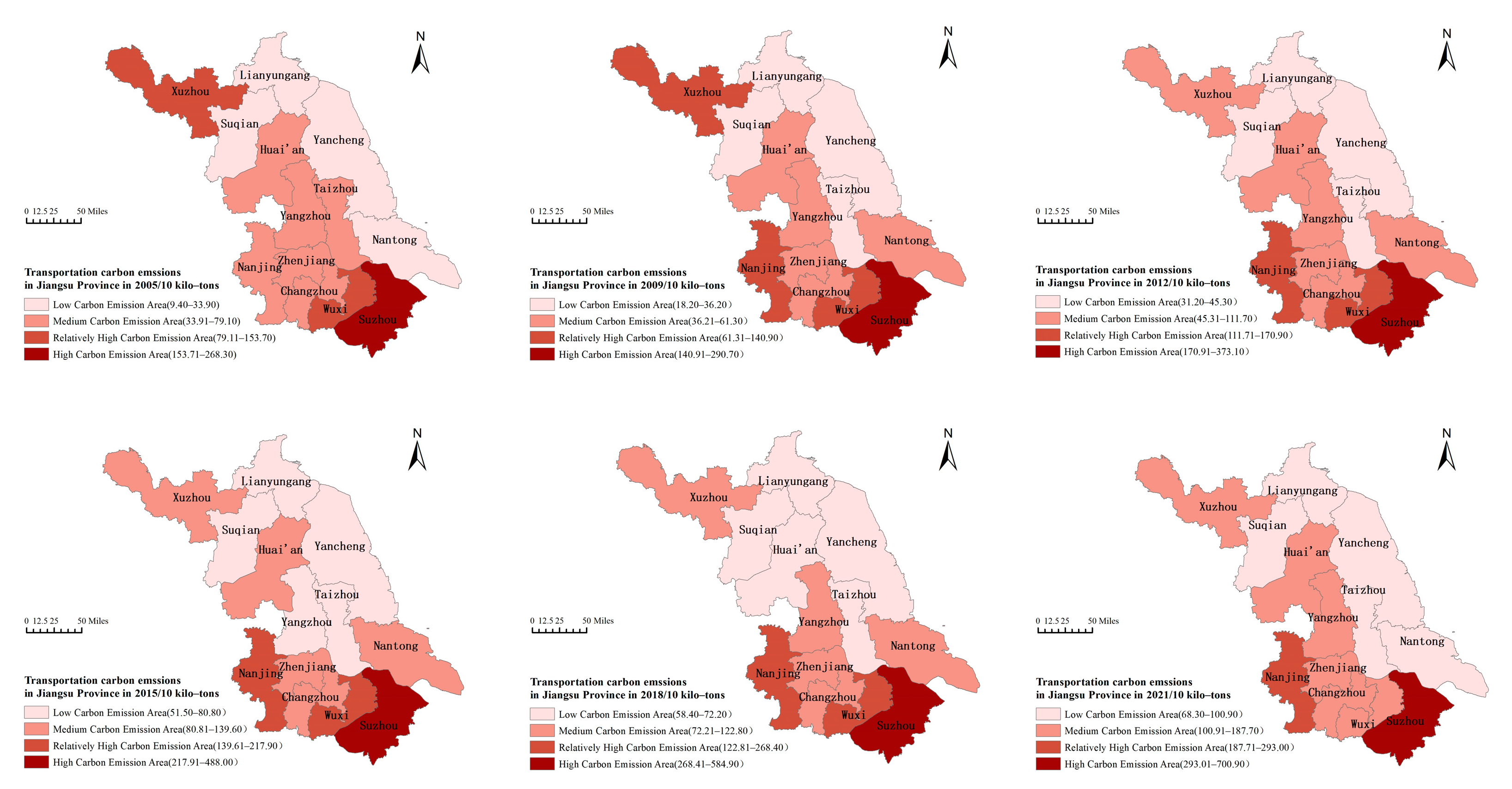
• Transport carbon emissions in Jiangsu Province have maintained a continuous upward trend since 2000 but experienced fluctuations after 2019. This study utilized the STIRPAT model as a basis to select eight influencing factors for analysis and prediction since 2000: total population, per capita GDP, motor vehicle ownership, passenger turnover, cargo turnover, urbanization rate, urban green space coverage, and carbon emission intensity. To overcome the adverse effects of variable multicollinearity in the modeling process, this study used principal component analysis to decompose the original eight variables and extract the principal components to establish a regression model. Four principal components were eventually resolved, and the value is 99.628, which explains the model well.
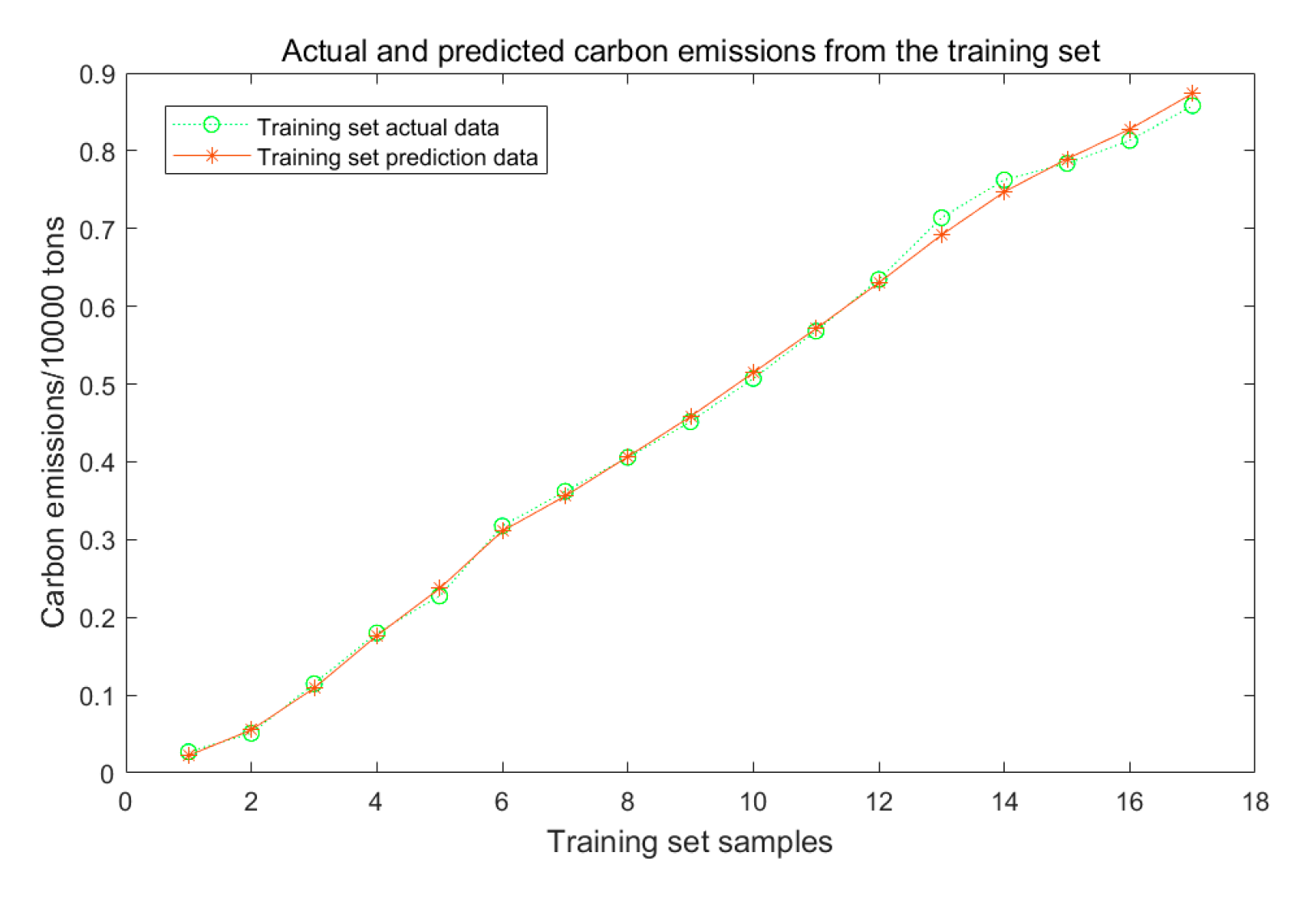
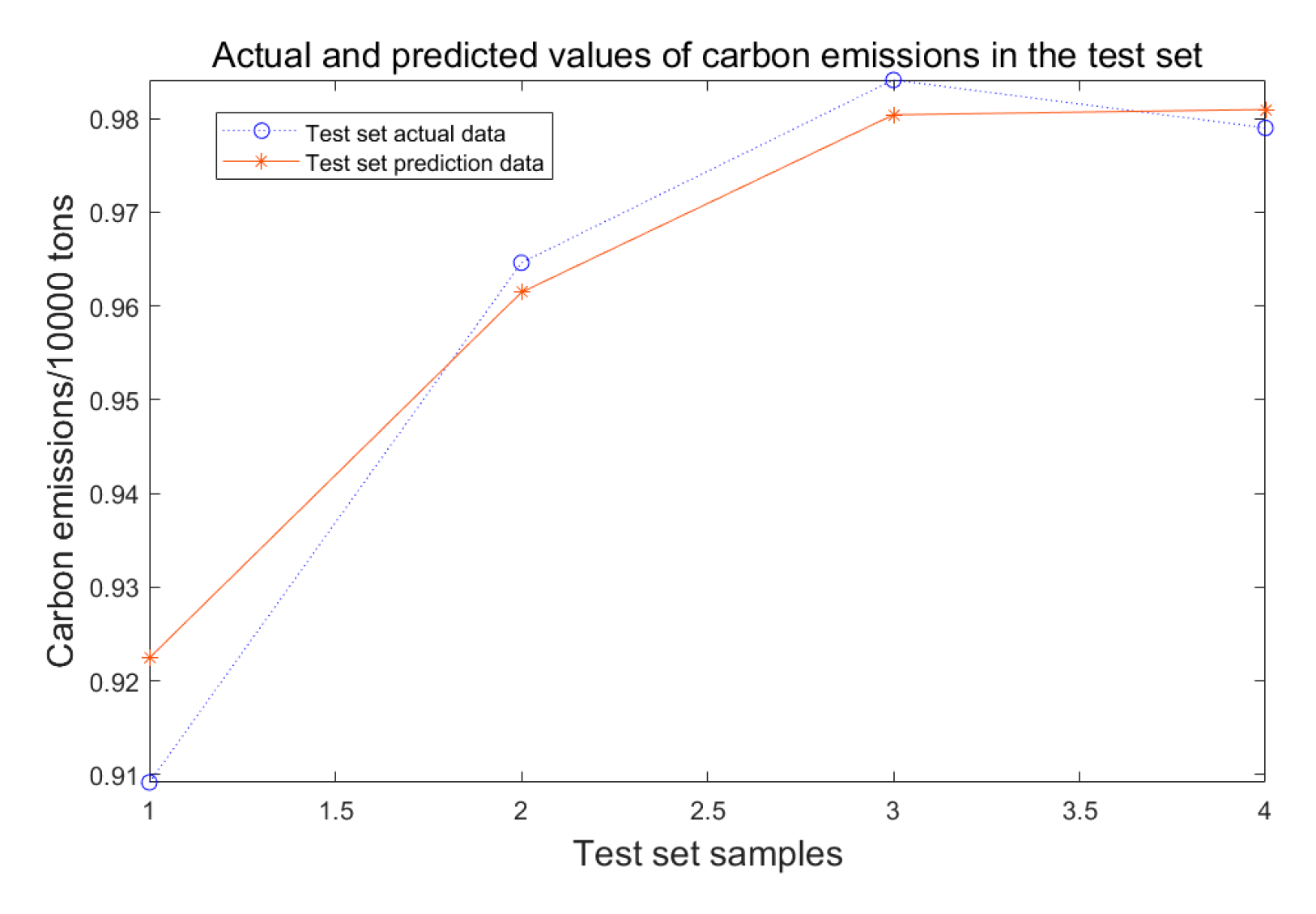
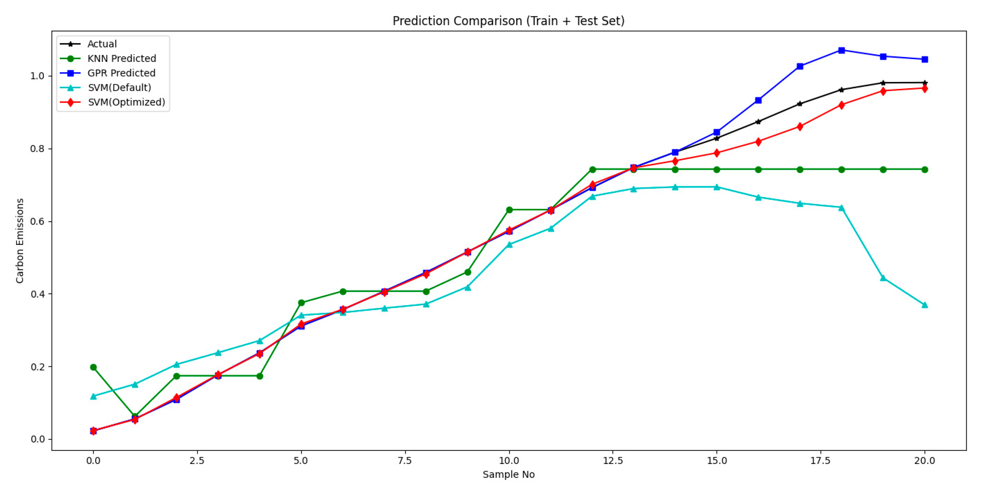
• This study conducted an error comparison analysis on the SVM, KNN, GPR, and WOA-SVM prediction models to ensure the accuracy and scientific nature of the research results. The results show that the coefficient of determination (R²) for the WOA-SVM model reached 0.91. It also indicates that the relative errors between simulated and actual carbon emission values remained within 1.5% across all years. These results show that the WOA-SVM model of this study is significantly better than other prediction models in terms of error and correlation coefficient evaluation indicators, thereby improving the credibility of the prediction results.
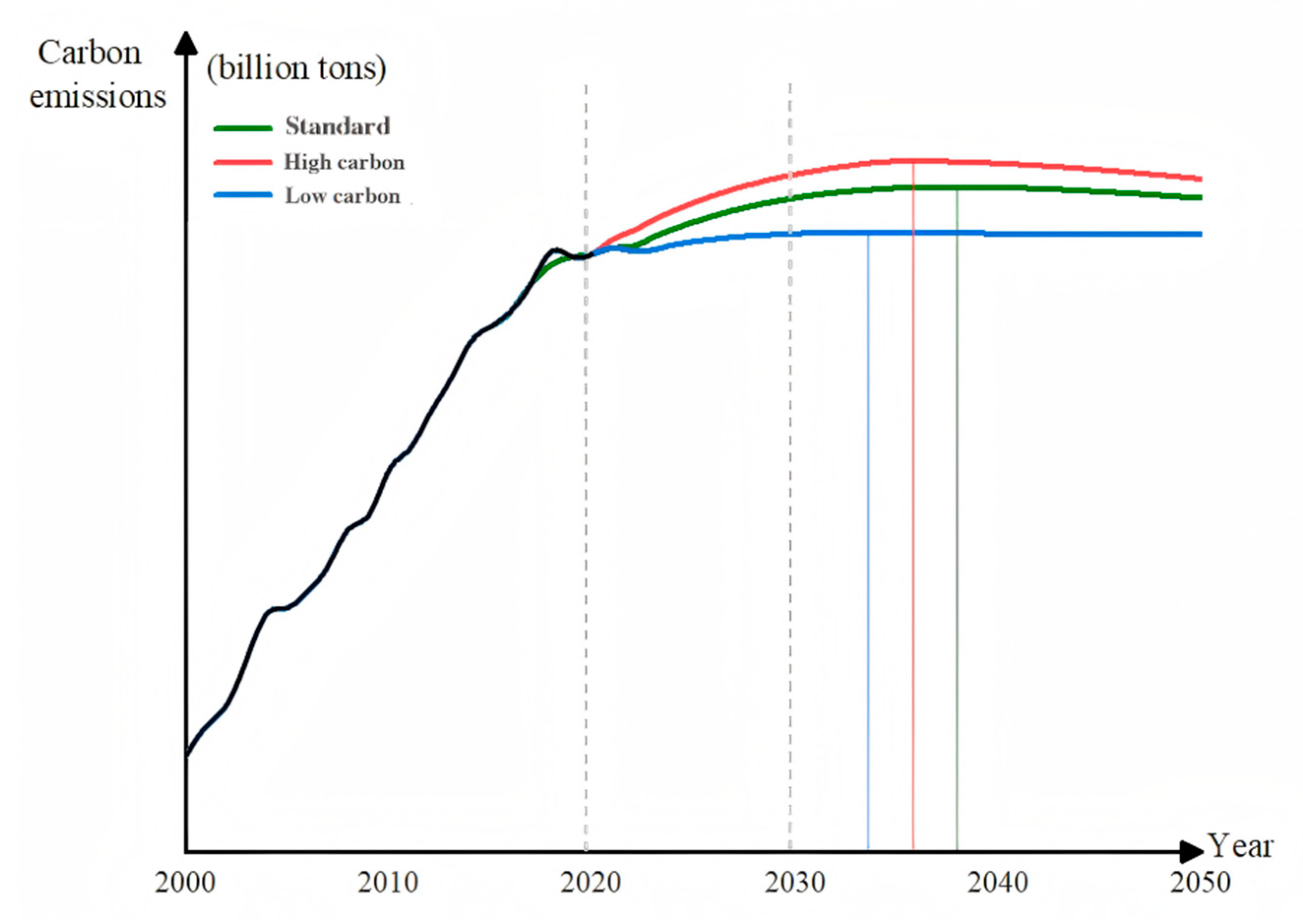
• This study conducted a scenario-based forecasting analysis. The results indicate that carbon emissions from the transportation sector in Jiangsu Province are projected to experience slow growth, followed by a carbon peak, after which a sustained decline is expected. Further comparisons reveal that under the baseline scenario, emissions will increase at a low rate until reaching peak levels in 2038. By contrast, under the high-carbon scenario, emissions will increase at a faster pace, peaking in 2036. Under the low-carbon scenario, emission growth will slow further, stabilize earlier, and achieve peak status in 2034, which is closest to the official carbon peak target. Therefore, proactive emission reduction measures and low-carbon policies can significantly reduce carbon emissions and promote sustainable development.

However, this study has some limitations that should be acknowledged. Owing to data availability constraints, this study primarily relies on statistical yearbooks and government-released datasets. Although these sources are authoritative, their limitations include low spatiotemporal resolution, delayed updates, and a lack of cross-validation with multi-source heterogeneous data (e.g., satellite remote sensing, land-use data). Such limitations may introduce quantification biases in key driving factors. Furthermore, existing datasets fail to incorporate 3D indicators, such as building height and density, thereby hindering the exploration of vertical spatial development’s impact mechanisms on carbon emissions and limiting the model’s responsiveness to multidimensional dynamics.

Future research directions may focus on the following aspects:

• Establish a cross-regional, multimodal transportation carbon emission database by integrating satellite remote sensing data, real-time traffic monitoring data, and granular energy consumption data. This method will enhance the model’s capacity to characterize complex systems and construct a “space–society–energy” multidimensional data cube.
• Incorporate 3D urban indicators to improve the model’s precision in delineating urban morphology–carbon emission correlations.
• Develop an adaptive fusion framework by introducing dynamic weights during the WOA encircling predation phase. This strategy will enable the dynamic adjustment of WOA-SVM weights, thereby enhancing fitting accuracy for non-stationary, multimodal carbon emission trends.
• Conduct comparative experiments across multiple Chinese provinces to identify the model’s applicability boundaries in regions with diverse economic structures and resource endowments, thereby establishing region-specific prediction paradigms.

References

1. Nishioka, S. A challenge for sustainability science: Can we halt climate change? Sustain. Sci. 2024, 19, 7–18. [Google Scholar] [CrossRef]
2. Li, C.; Zhang, Z.; Wang, L. Carbon peak forecast and low carbon policy choice of transportation industry in China: Scenario prediction based on STIRPAT model. Environ. Sci. Pollut. Res. 2023, 30, 63250–63271. [Google Scholar] [CrossRef] [PubMed]
3. Eslamipoor, R. Contractual Mechanisms for Coordinating a Sustainable Supply Chain With Carbon Emission Reduction. Bus. Strategy Environ. 2025. [Google Scholar] [CrossRef]
4. Sepehriar, A.; Eslamipoor, R. An economical single-vendor single-buyer framework for carbon emission policies. J. Bus. Econ. 2024, 94, 927–945. [Google Scholar] [CrossRef]
5. Xu, A.; Song, M.; Wu, Y.; Luo, Y.; Zhu, Y.; Qiu, K. Effects of new urbanization on China’s carbon emissions: A quasi-natural experiment based on the improved PSM-DID model. Technol. Forecast. Soc. Change 2024, 200, 123164. [Google Scholar] [CrossRef]
6. Macioszek, E.; Granà, A.; Fernandes, P.; Coelho, M.C. New Perspectives and Challenges in Traffic and Transportation Engineering Supporting Energy Saving in Smart Cities—A Multidisciplinary Approach to A Global Problem; MDPI: Basel, Switzerland, 2022; Volume 15, p. 4191. [Google Scholar]
7. Zhu, H.; Cao, S.; Su, Z.; Zhuang, Y. China’s future energy vision: Multi-scenario simulation based on energy consumption structure under dual carbon targets. Energy 2024, 301, 131751. [Google Scholar] [CrossRef]
8. Jin, Y.; Sharifi, A.; Li, Z.; Chen, S.; Zeng, S.; Zhao, S. Carbon emission prediction models: A review. Sci. Total Environ. 2024, 2024, 172319. [Google Scholar] [CrossRef]
9. Sun, X.; Zhang, X. Assessment and Driving Factors of Embodied Carbon Emissions in the Construction Sector: Evidence from 2005 to 2021 in Northeast China. Sustainability 2024, 16, 5681. [Google Scholar] [CrossRef]
10. Li, Y.; Yang, X.; Du, E.; Liu, Y.; Zhang, S.; Yang, C.; Zhang, N.; Liu, C. A review on carbon emission accounting approaches for the electricity power industry. Appl. Energy 2024, 359, 122681. [Google Scholar] [CrossRef]
11. Liu, Y.; Liu, J.; Huang, C. Characteristics of Spatial Network Structure of Transportation Carbon Emission and Influencing Factors in Yangtze River Economic Belt. Environ. Sci. Manag. 2024, 49, 45–49+65. [Google Scholar]
12. Xu, X.; Xu, H. The driving factors of carbon emissions in China’s transportation sector: A spatial analysis. Front. Energy Res. 2021, 9, 664046. [Google Scholar] [CrossRef]
13. Pan, X.; Guo, S.; Xu, H.; Tian, M.; Pan, X.; Chu, J. China’s carbon intensity factor decomposition and carbon emission decoupling analysis. Energy 2022, 239, 122175. [Google Scholar] [CrossRef]
14. Wang, H.; Shi, W.; He, W.; Xue, H.; Zeng, W. Simulation of urban transport carbon dioxide emission reduction environment economic policy in China: An integrated approach using agent-based modelling and system dynamics. J. Clean. Prod. 2023, 392, 136221. [Google Scholar] [CrossRef]
15. Yan, J.; Su, B.; Liu, Y. Multiplicative structural decomposition and attribution analysis of carbon emission intensity in China, 2002–2012. J. Clean. Prod. 2018, 198, 195–207. [Google Scholar] [CrossRef]
16. Shang, W.-L.; Ling, Y.; Ochieng, W.; Yang, L.; Gao, X.; Ren, Q.; Chen, Y.; Cao, M. Driving forces of CO2 emissions from the transport, storage and postal sectors: A pathway to achieving carbon neutrality. Appl. Energy 2024, 365, 123226. [Google Scholar] [CrossRef]
17. Rasool, Y.; Zaidi, S.A.H.; Zafar, M.W. Determinants of carbon emissions in Pakistan’s transport sector. Environ. Sci. Pollut. Res. 2019, 26, 22907–22921. [Google Scholar] [CrossRef]
18. Fan, F.; Lei, Y. Decomposition analysis of energy-related carbon emissions from the transportation sector in Beijing. Transp. Res. Part D Transp. Environ. 2016, 42, 135–145. [Google Scholar] [CrossRef]
19. Ziyuan, C.; Yibo, Y.; Simayi, Z.; Shengtian, Y.; Abulimiti, M.; Yuqing, W. Carbon emissions index decomposition and carbon emissions prediction in Xinjiang from the perspective of population-related factors, based on the combination of STIRPAT model and neural network. Environ. Sci. Pollut. Res. 2022, 29, 31781–31796. [Google Scholar] [CrossRef]
20. Yin, F.; Bo, Z.; Yu, L.; Wang, J. Prediction of carbon dioxide emissions in China using a novel grey model with multi-parameter combination optimization. J. Clean. Prod. 2023, 404, 136889. [Google Scholar] [CrossRef]
21. Ning, L.; Pei, L.; Li, F. Forecast of China’s carbon emissions based on Arima method. Discret. Dyn. Nat. Soc. 2021, 2021, 1441942. [Google Scholar] [CrossRef]
22. Çevik, A.; Kurtoğlu, A.E.; Bilgehan, M.; Gülşan, M.E.; Albegmprli, H.M. Support vector machines in structural engineering: A review. J. Civ. Eng. Manag. 2015, 21, 261–281. [Google Scholar] [CrossRef]
23. Tavara, S. Parallel computing of support vector machines: A survey. ACM Comput. Surv. (CSUR) 2019, 51, 1–38. [Google Scholar] [CrossRef]
24. Leong, W.; Kelani, R.; Ahmad, Z. Prediction of air pollution index (API) using support vector machine (SVM). J. Environ. Chem. Eng. 2020, 8, 103208. [Google Scholar] [CrossRef]
25. Saleh, C.; Dzakiyullah, N.R.; Nugroho, J.B. Carbon Dioxide Emission Prediction Using Support Vector Machine; IOP Conference Series: Materials Science and Engineering; IOP Publishing: Bristol, UK, 2016; p. 012148. [Google Scholar]
26. Mladenović, I.; Sokolov-Mladenović, S.; Milovančević, M.; Marković, D.; Simeunović, N. Management and estimation of thermal comfort, carbon dioxide emission and economic growth by support vector machine. Renew. Sustain. Energy Rev. 2016, 64, 466–476. [Google Scholar] [CrossRef]
27. Zhou, J.; Zhu, S.; Qiu, Y.; Armaghani, D.J.; Zhou, A.; Yong, W. Predicting tunnel squeezing using support vector machine optimized by whale optimization algorithm. Acta Geotech. 2022, 17, 1343–1366. [Google Scholar] [CrossRef]
28. Zhou, W.; Lian, J.; Zhang, J.; Mei, Z.; Gao, Y.; Hui, G. Tomato storage quality predicting method based on portable electronic nose system combined with WOA-SVM model. J. Food Meas. Charact. 2023, 17, 3654–3664. [Google Scholar] [CrossRef]
29. Guo, H.; Wu, L.; Wang, X.; Xing, X.; Zhang, J.; Qing, S.; Zhao, X. Optimization of Support Vector Machine with Biological Heuristic Algorithms for Estimation of Daily Reference Evapotranspiration Using Limited Meteorological Data in China. Agronomy 2024, 14, 1780. [Google Scholar] [CrossRef]
30. Wu, R.; Wang, J.; Wang, S.; Feng, K. The drivers of declining CO2 emissions trends in developed nations using an extended STIRPAT model: A historical and prospective analysis. Renew. Sustain. Energy Rev. 2021, 149, 111328. [Google Scholar] [CrossRef]
31. Li, B.; Liu, X.; Li, Z. Using the STIRPAT model to explore the factors driving regional CO 2 emissions: A case of Tianjin, China. Nat. Hazards 2015, 76, 1667–1685. [Google Scholar] [CrossRef]
32. Zhu, C.; Wang, M.; Du, W. Prediction on peak values of carbon dioxide emissions from the Chinese transportation industry based on the SVR model and scenario analysis. J. Adv. Transp. 2020, 2020, 8848149. [Google Scholar] [CrossRef]
33. Zhu, C.; Yang, S.; Liu, P. Study on the factors influencing on the carbon emissions of Shaanxi Province’s transportation industry in China. Sustainability 2022, 14, 8610. [Google Scholar] [CrossRef]
34. Xu, B.; Lin, B. Factors affecting carbon dioxide (CO2) emissions in China’s transport sector: A dynamic nonparametric additive regression model. J. Clean. Prod. 2015, 101, 311–322. [Google Scholar] [CrossRef]
35. Niu, H.; Zhang, Z.; Xiao, Y.; Luo, M.; Chen, Y. A study of carbon emission efficiency in Chinese provinces based on a three-stage SBM-undesirable model and an LSTM model. Int. J. Environ. Res. Public Health 2022, 19, 5395. [Google Scholar] [CrossRef]
36. Wang, P.; Wu, W.; Zhu, B.; Wei, Y. Examining the impact factors of energy-related CO2 emissions using the STIRPAT model in Guangdong Province, China. Appl. Energy 2013, 106, 65–71. [Google Scholar] [CrossRef]
37. Eggleston, H.; Buendia, L.; Miwa, K.; Ngara, T.; Tanabe, K. 2006 IPCC Guidelines for National Greenhouse Gas Inventories; IGES: Kanagawa, Japan, 2006. [Google Scholar]
38. Miao, A.; Yuan, Y.; Wu, H.; Ma, X.; Shao, C.; Xiang, S. Pathway for China’s provincial carbon emission peak: A case study of the Jiangsu Province. Energy 2024, 298, 131417. [Google Scholar] [CrossRef]
39. Mirjalili, S.; Lewis, A. The whale optimization algorithm. Adv. Eng. Softw. 2016, 95, 51–67. [Google Scholar] [CrossRef]
40. Zhang, R.; Liu, M.; Pan, Z.; Yin, Y. Network security situation assessment based on improved WOA-SVM. IEEE Access 2022, 10, 96273–96283. [Google Scholar] [CrossRef]
41. Cheng, Y.; Gai, X.; Jin, Y.; Guan, R.; Lu, M.; Ding, Y. A new method based on a WOA-optimized support vector machine to predict the tool wear. Int. J. Adv. Manuf. Technol. 2022, 121, 6439–6452. [Google Scholar] [CrossRef]
42. Elkorany, A.S.; Marey, M.; Almustafa, K.M.; Elsharkawy, Z.F. Breast cancer diagnosis using support vector machines optimized by whale optimization and dragonfly algorithms. IEEE Access 2022, 10, 69688–69699. [Google Scholar] [CrossRef]
43. Suthaharan, S.; Suthaharan, S. Support vector machine. In Machine Learning Models and Algorithms for Big Data Classification: Thinking with Examples for Effective Learning; Springer US: Boston, MA, USA, 2016; pp. 207–235. [Google Scholar]
44. Mun, S.; Park, S.; Han, D.K.; Ko, H. Generative Adversarial Network Based Acoustic Scene Training Set Augmentation and Selection Using SVM Hyper-Plane; DCASE: Barcelona, Spain, 2017; pp. 93–102. [Google Scholar]
45. Liu, W.; Ren, Y.; Meng, X.; Tian, B.; Lv, X. Analysis of potential water inflow rates at an underground coal mine using a WOA-CNN-SVM approach. Water 2024, 16, 813. [Google Scholar] [CrossRef]
46. Cong, Y.; Hou, L.; Wu, Y.; Ma, Y. Development of a Coupled EnergyPlus—MATLAB Simulation Based on LSTM for Predictive Control of HVAC System. Math. Probl. Eng. 2022, 2022, 5912967. [Google Scholar] [CrossRef]
47. Xie, P.; Liao, J.; Pan, X.; Sun, F. Will China’s carbon intensity achieve its policy goals by 2030? Dynamic scenario analysis based on STIRPAT-PLS framework. Sci. Total Environ. 2022, 832, 155060. [Google Scholar] [CrossRef]
48. Yi, X.; Jue, W.; Huan, H. Does economic development bring more livability? Evidence from Jiangsu Province, China. J. Clean. Prod. 2021, 293, 126187. [Google Scholar] [CrossRef]
49. Lu, Q.; Chai, J.; Wang, S.; Zhang, Z.G.; Sun, X.C. Potential energy conservation and CO2 emissions reduction related to China’s road transportation. J. Clean. Prod. 2020, 245, 118892. [Google Scholar] [CrossRef]
50. Wang, J.; Xie, X.; Liu, W.; Li, Y.; Li, Y.; Xing, W. Analyses of carbon dioxide emission peak and reduction potential for Shandong transportation through multi-scenario simulation. Environ. Pollut. Control. 2023, 13, 13684. [Google Scholar]
51. He, W.; Li, X.; Yang, J.; Ni, H.; Sang, X. How land use functions evolve in the process of rapid urbanization: Evidence from Jiangsu Province, China. J. Clean. Prod. 2022, 380, 134877. [Google Scholar] [CrossRef]
52. Tang, D.; Ma, T.; Li, Z.; Tang, J.; Bethel, B.J. Trend prediction and decomposed driving factors of carbon emissions in Jiangsu Province during 2015–2020. Sustainability 2016, 8, 1018. [Google Scholar] [CrossRef]
53. Huang, Z.; Ji, L.; Yin, J.; Lü, C.; Wang, J.; Yin, H.; Ding, Y.; Cai, B.; Yan, G. Peak Pathway of China’s Road Traffic Carbon Emissions. Res. Environ. Sci. 2022, 35, 385–393. [Google Scholar]
54. Wang, H.; Zhang, H. Prediction of China’s Carbon Emission Intensity Based on a Grey Breakpoint Model with Inverse Accumulation. Environ. Sci. 1–21, preprint. [CrossRef]
55. Xiong, S.; Yuan, Y.; Zhang, C. Achievement of carbon peak goals in China’s road transport—Possibilities and pathways. J. Clean. Prod. 2023, 388, 135894. [Google Scholar] [CrossRef]
Figure 1. Diagram of the encirclement attack.
Sustainability 17 04612 g001
Figure 2. Diagram of the bubble network attack.
Sustainability 17 04612 g002
Figure 3. Total carbon emissions from the transportation industry in Jiangsu Province during six selected years between 2005 and 2021.
Sustainability 17 04612 g003
Figure 4. Actual and predicted carbon emissions from the training set.
Sustainability 17 04612 g004
Figure 5. Actual and predicted carbon emissions from the test set.
Sustainability 17 04612 g005
Figure 6. Comparative analysis of the prediction performance of the four models.
Sustainability 17 04612 g006
Figure 7. Future trends in carbon emissions from the transportation industry under different scenarios.
Sustainability 17 04612 g007