A Framework for Optimal Parameter Selection in Electrocoagulation Wastewater Treatment Using Integrated Physics-Based and Machine Learning Models

Abstract

Electrocoagulation (EC) systems are regaining attention as a promising wastewater treatment technology due to their numerous advantages, including low system and operational costs and environmental friendliness. However, the widespread adoption and further development of EC systems have been hindered by a lack of fundamental understanding, necessitating systematic research to provide essential insights for system developers. In this study, a continuous EC system with a realistic setup is analyzed using an unsteady, two-dimensional physics-based model that incorporates multiphysics. The model captures key mechanisms, such as arsenic adsorption onto flocs, electrochemical reactions at the electrodes, chemical reactions in the bulk solution, and ionic species transport via diffusion and convection. Additionally, it accounts for bulk wastewater flow circulating between the EC cell and an external storage tank. This comprehensive modeling approach enables a fundamental analysis of how operating conditions influence arsenic removal efficiency, providing crucial insights for optimizing system utilization. Furthermore, the developed model is used to generate data under various operating conditions. Seven machine learning models are trained on this data after hyperparameter optimization. These high-accuracy models are then employed to develop processing maps that identify the conditions necessary to achieve acceptable removal efficiency. This study is the first to generate processing maps by synergistically integrating physics-based and data-driven models. These maps provide clear design and operational guidelines, helping researchers and engineers optimize EC systems. This research establishes a framework for combining physics-based and data-driven modeling approaches to generate processing maps that serve as essential guidelines for wastewater treatment applications.

1. Introduction

Electrocoagulation (EC) is an innovative wastewater treatment system that leverages the large surface area of flocs generated during operation to extract dissolved contaminants from wastewater. Unlike traditional chemical coagulation systems, EC produces the required amount of coagulants without the need for external additives. This eliminates the risk of secondary contamination caused by improper dosing of coagulants, making EC an environmentally friendly alternative. A detailed review of various wastewater treatment systems, including their advantages and disadvantages, can be found in refs. [1,2,3].

The EC system has a simple structure, consisting of metal electrodes, and operates solely on electricity without requiring high levels of operational expertise. Due to these advantages, EC has been widely applied to treat various types of wastewater, including those containing heavy metals [4], organic compounds [5], phosphate [6], fluoride [7], arsenic [8,9,10], and chemical–mechanical polishing wastewater [11,12].

Despite its benefits, EC has not been fully adopted on a large scale due to challenges related to performance efficiency and scaling up [13,14]. However, with increasing environmental concerns, interest in EC technology is growing. Most current applications are limited to small- and medium-scale operations [14], highlighting the need for further fundamental research to better understand the system, overcome existing challenges, and expand its full-scale implementation.

It has been reported that there are 75 manufacturers of electrocoagulation (EC) systems worldwide [15]. The United States holds approximately 33% of the global EC manufacturing market and is considered the leader in EC innovation, contributing nearly 59% of advanced design developments. Among various configurations, a two-stage process combining electrocoagulation (EC) and electro-oxidation (EO) has demonstrated the highest performance in industrial wastewater treatment, accounting for 54% of all hybrid systems globally. Most commercial EC systems are small to medium in scale, representing 88% of all systems currently available worldwide. Comprehensive data are available in ref. [15] on global EC manufacturers, including the types of industrial EC reactor cells, production capacities, and a detailed list of industrial applications covering wastewater types, contaminants treated, treatment volumes, electrode materials, removal efficiencies, and corresponding companies and countries.

The challenges associated with scaling up EC systems for industrial applications can be broadly categorized into two main factors [2,13,14]: high operational and management costs, and low system performance. One major barrier to full-scale implementation is the high electricity consumption. Additionally, low performance and poor long-term operational stability remain significant concerns. Performance failures have been reported in pilot-scale studies, potentially due to factors such as electrode degradation, floc clogging, insufficient biofilm formation, and reduced microbial activity. Addressing these challenges requires a clear understanding of the underlying mechanisms of EC system operation. This highlights the importance of fundamental research aimed at identifying key control parameters and elucidating removal mechanisms through a multiphysics approach.

Research based on mathematical modeling has been conducted to gain deeper insight into the electrocoagulation (EC) system, aiming for a fundamental understanding of the multiphysics processes that characterize EC and the influence of key parameters on its performance. Various modeling approaches have been employed, including lumped-parameter models [16,17,18,19,20], multiphysics models with mass transfer [21,22], electrochemical models [23,24], statistical models [25,26,27], and machine learning models [28,29,30].

The lumped-parameter model [16,17,18,19,20] assumes a uniform distribution of chemical species, such as ions, coagulants, and contaminants, within the cell. Consequently, it does not account for spatial variations in species concentration during EC operation. This assumption is valid for well-mixed batch reactors, leading to a zero-dimensional modeling approach. While this method is relatively simple and avoids the complexities of multiphysics calculations, including electrochemical and chemical reactions, mass transfer, and fluid dynamics, its parameters are highly dependent on specific experimental conditions. As a result, it is limited to certain systems and lacks the ability to provide deeper physical insights into EC processes.

To overcome the limitations of lumped-parameter models, multiphysics models incorporating mass transfer have been developed [21,22]. These models account for the diffusion and convection of chemical species and their impact on chemical and electrochemical reactions. However, most studies utilizing this approach focus on steady-state conditions and do not capture the dynamic behavior of chemical species within the EC system [21]. Additionally, adsorption physics, which plays a crucial role in contaminant removal, is often overlooked [21,22]. Consequently, these models fail to describe how the distribution of ionic species influences pollutant removal rates.

Electrochemical models have been developed to establish a relationship between electrical potential and current in continuous parallel-plate EC systems used for drinking water treatment [23]. These models address the limitations of conventional EC models, which tend to focus on pollutant removal without giving adequate attention to the underlying electrochemical mechanisms. By solving potential and energy balances at each equipotential segment, these models consider the contributions of ionic concentration, solution temperature and conductivity, cathodic hydrogen flux, and the gas/liquid ratio [23,24]. However, they do not incorporate coagulation processes and their effects on pollutant removal.

Statistical models [25,26,27] have been applied to analyze experimental data and optimize EC operating conditions. The response surface methodology (RSM) has been used to evaluate the effects of independent variables, such as applied current density, electrolyte concentration, electrolysis duration, and pH, on pollutant removal efficiency. For example, empirical relationships have been established for arsenic removal using aluminum and steel anodes [25]. Similarly, RSM has been applied to optimize EC processes for the removal of C.I. Reactive Red 43 considering parameters like current density, treatment duration, pH, and chloride concentration [26]. In some cases, removal efficiencies exceeding 99% have been achieved under optimal conditions. However, despite their predictive capabilities, statistical models do not provide fundamental physical insights into EC processes.

Machine learning (ML) approaches [28,29,30] have been increasingly utilized to develop predictive models for EC performance. For instance, M. Akoulih et al. [28] employed deep learning to predict azo dye removal rates, while P. B. Bhagawati et al. [29] used both linear regression and artificial neural networks to predict biochemical oxygen demand (BOD), chemical oxygen demand (COD), and chromium concentration in treated effluents. Additionally, M. G. Shirkoohi et al. [30] compared various artificial intelligence models for predicting phosphate removal efficiency from wastewater using EC. Techniques such as adaptive neuro-fuzzy inference systems, artificial neural networks, and support vector regression were applied, with the key input variables including current intensity, initial phosphate concentration, pH, treatment duration, and electrode type. Optimal hyperparameters were identified to enhance the reliability and robustness of these ML models. Among the findings, the electrode type and initial phosphate concentration emerged as the most influential factors affecting phosphate removal efficiency. Machine learning is one of the most effective approaches for correlating highly nonlinear parameters and identifying optimal conditions; however, it lacks the ability to provide physical insights into how these parameters influence the performance of the electrochemical (EC) system.

Recently, our research group reported [31], for the first time, a comprehensive EC model that incorporates all the essential physical processes, providing deeper insights into EC mechanisms. This two-dimensional, time-dependent model integrates electrochemical reactions at the electrode surface, chemical reactions in the bulk solution, mass transfer via diffusion and convection, and pollutant removal by coagulated flocs. This study provides a detailed understanding of how chemical species evolve and distribute within the EC system under various operating conditions, offering a physics-based explanation of how these conditions influence pollutant removal rates.

In this study, we aim to build upon our previous work by further refining the EC model to simulate near-realistic operating conditions. Most existing studies focus on well-mixed batch systems (zero-dimensional models) or single-pass continuous-flow systems, which do not simulate realistic conditions but help elucidate reaction dynamics within EC. In this study, we introduce a recirculation system in which wastewater is continuously treated as it cycles between the EC cell and a storage tank, simulating realistic operating conditions. The resulting data are used to train machine learning models for predicting EC performance under various conditions. Additionally, this data-driven approach facilitates the creation of a process optimization map, which can guide the design and operational strategies for EC systems to enhance their effectiveness.

The modeling approach presented here is generalizable and can be applied to various types of pollutants. This fundamental research aims to provide insight into the reaction mechanisms within the electrocoagulation (EC) process and establishes a framework for integrating physics-based models with machine learning to analyze the effects of processing parameters on removal efficiency. The proposed framework is not limited to arsenic removal but is designed to be applicable to a wide range of industrial pollutants, offering theoretical guidance for broader EC applications.

2. Methodology

A typical electrocoagulation (EC) test setup, consisting of continuous parallel-plate EC systems, developed in our lab is shown in Figure 1a as an example. The system comprises an EC cell, an external tank, a pump, flexible tubing, and a power supply. Wastewater is pumped from the external tank into the EC cell, where pollutants are removed through floc formation induced by the electrocoagulation process. Figure 1b illustrates an example of pollutant-floc agglomerates that have settled as a result of electrocoagulation. The treated solution then returns to the external tank, where it mixes with untreated wastewater before being recirculated back to the EC cell. This cycle repeats until the pollutant concentration reaches the desired level.

2.1. Development of Physics-Based Model

In this study, the electrocoagulation (EC) process for treating arsenic-contaminated wastewater is analyzed using a two-dimensional, time-dependent mathematical model, which is validated against experimental data from the literature [16]. This model incorporates multiple physical phenomena, including electrochemical reactions at the electrode surfaces, chemical reactions in the solution, wastewater flow dynamics, ionic species mass transfer by diffusion and convection, and the physical adsorption of arsenics into the coagulated flocs.

Figure 2 illustrates the simplified structure used to develop the model. This modeling study is based on a lab-scale system utilizing well-characterized wastewater samples, enabling a fundamental investigation of electrochemical reactions. The insights gained can serve as a theoretical foundation for analyzing real industrial wastewater, which is typically far more complex and contains a wide range of contaminants. These pollutants are commonly quantified using indices such as BOD, COD, and TDS. Detailed information on industrial effluents and their pollution characteristics can be found in refs. [1,2,3].

2.1.1. Governing Equations

• Electrode Reactions (Electrochemical Reaction)

When an electric current is applied to the electrodes, chemical ionic species are generated at the electrode surfaces through electrochemical reactions. Aluminum ions (Al³⁺) are released from the aluminum anode (+ electrode, (5) in Figure 2) via oxidation, while hydroxide ions (OH⁻) are produced at the cathode (− electrode, (6) in Figure 2) through a water-splitting reduction reaction. These electrochemical reactions are described in Equations (1) and (2). The generation rate of these ionic species is directly proportional to the applied current.

$$\mathrm{Anode}: Al\to A{l}^{3+}+3e^{-}$$

(1)

$$\mathrm{Cathode}: 2H_{2}O+2e^{-}\to H_2+2O{H}^{-}$$

(2)

• Chemical Reactions

Ionic species generated in electrochemical reaction undergo a series of chemical reactions in a solution to produce various species of aluminum hydroxide, such as $Al{\left(OH\right)}^{2+}$, $Al{\left(OH\right)}_2^{+}$, $Al{\left(OH\right)}_3$, and $Al{\left(OH\right)}_4^{-}$, as described in Equations (3)–(7) [4,16].

$$A{l}^{3+}+H_{2}O\underset{k_{1-b}}{\stackrel{k_{1-f}}{\rightleftharpoons }}Al{\left(OH\right)}^{2+}+H^{+}$$

(3)

$$Al{\left(OH\right)}^{2+}+H_{2}O\underset{k_{2-b}}{\stackrel{k_{2-f}}{\rightleftharpoons }}Al{\left(OH\right)}_2^{+}+H^{+}$$

(4)

$$Al{\left(OH\right)}_2^{+}+H_{2}O\underset{k_{3-b}}{\stackrel{k_{3-f}}{\rightleftharpoons }}Al{\left(OH\right)}_3+H^{+}$$

(5)

$$Al{\left(OH\right)}_3+H_{2}O\underset{k_{4-b}}{\stackrel{k_{4-f}}{\rightleftharpoons }}Al{\left(OH\right)}_4^{-}+H^{+}$$

(6)

$$H_{2}O\underset{k_{w-b}}{\stackrel{k_{w-f}}{\rightleftharpoons }}{H}^{+}+O{H}^{-}$$

(7)

The reaction rates (R) of the chemical reactions above depend upon the concentrations of the products and reactants and the reaction rate constant (k) for each reaction, and they are described in Equations (8)–(12) [16,21].

$$R_1=k_{1-f}\left(\left[{Al}^{3+}\right]-{\displaystyle \frac{\left[{Al\left(OH\right)}^{2+}\right]·\left[H^{+}\right]}{K_1}}\right)$$

(8)

$$R_2=k_{2-f}\left(\left[{Al\left(OH\right)}^{2+}\right]-{\displaystyle \frac{\left[{Al\left(OH\right)}_2^{+}\right]·\left[H^{+}\right]}{K_2}}\right)$$

(9)

$$R_3=k_{3-f}\left(\left[{Al\left(OH\right)}_2^{+}\right]-{\displaystyle \frac{\left[{Al\left(OH\right)}_3\right]·\left[H^{+}\right]}{K_3}}\right)$$

(10)

$$R_4=k_{4-f}\left(\left[{Al\left(OH\right)}_3\right]-{\displaystyle \frac{\left[{Al\left(OH\right)}_4^{-}\right]·\left[H^{+}\right]}{K_4}}\right)$$

(11)

$$R_w=k_{wf}\left(1-{\displaystyle \frac{\left[{OH}^{-}\right]·\left[H^{+}\right]}{K_w}}\right)$$

(12)

• Mass Balance Equations

Concentrations of the chemical species are dynamically changed during cell operation, and the change rate can be calculated by the following equations [16].

$${\displaystyle \frac{d\left[Al{\left(OH\right)}^{2+}\right]}{dt}}=R_1-R_2$$

(13)

$${\displaystyle \frac{d\left[Al{\left(OH\right)}_2^{+}\right]}{dt}}=R_2-R_3$$

(14)

$${\displaystyle \frac{d\left[Al{\left(OH\right)}_3\right]}{dt}}=R_4$$

(15)

$${\displaystyle \frac{d\left[Al{\left(OH\right)}_4^{-}\right]}{dt}}=R_3-R_4$$

(16)

$${\displaystyle \frac{d\left[H^{+}\right]}{dt}}=R_1+R_2+R_3+R_4+R_w$$

(17)

$${\displaystyle \frac{d\left[O{H}^{-}\right]}{dt}}=R_w$$

(18)

$${\displaystyle \frac{d\left[A{l}^{3+}\right]}{dt}}=-R_1$$

(19)

The concentration change rate of a chemical species is balanced by the mass transfer rate induced by diffusion and convection. The diffusion is driven by the concentration gradient in the cell, and convection is controlled by the bulk velocity [32].

$${\displaystyle \frac{\mathsf{\partial }{c}_i}{\mathsf{\partial }t}}=\mathsf{\nabla }·\left(-D\mathsf{\nabla }{c}_i+u{c}_i\right)$$

(20)

where $c_i$ is the concentration of species i (mol/m³), D is the diffusion coefficient, and u is the velocity field (m/s).

• Fluid Flow

The flow of wastewater in the cell is governed by momentum conservation equation. In this study, the wastewater is assumed to be ideal Newtonian fluid [21,22], and the Navier–Stokes equation, along with the continuity equation are used to analyze velocity and pressure distribution in the EC cell [33].

$$\rho {\displaystyle \frac{\mathsf{\partial }u}{\mathsf{\partial }t}}+\rho \left(u·\mathsf{\nabla }u\right)=\mathsf{\nabla }·\left[-pI+\kappa \right]+F$$

(21)

$$\rho \mathsf{\nabla }·u=0$$

(22)

where ρ is the density of the fluid (kg/m³), $u$ is the local velocity, $t$ is a time variable, p is pressure (Pa), $I$ is an identity matrix, κ is a viscous stress tensor (Pa), and F is a body force term (N).

• Saturation

Aluminum complex ions will precipitate, along with arsenic ions adsorbed on their surfaces, once their concentrations exceed the solubility limit of the solution. The saturation condition is described as a function of pH, based on the solubility diagram [34].

$${Al}_{sat}=K_s{K_w}^{-3}({10}^{-3pH}+K_{1s}·{10}^{-3pH}+K_{2s}·{10}^{-pH}+K_{3s}+K_{4s}·{10}^{pH})$$

(23)

• External Tank

As wastewater continuously circulates between the external tank and the EC cell (Figure 2), the concentration in the tank gradually changes. Treated species from the EC cell return to the tank, mixing with the existing solution and altering its composition. The rate of concentration change in the tank is determined using the following equation:

$${\displaystyle \frac{d{c}_i}{dt}}={\displaystyle \frac{L}{V}}\left({\int }_{outlet}\left(N_i·n\right)dS-{\int }_{inlet}\left(N_i·n\right)dS\right)$$

(24)

Here, $c_i$ represents the concentration of species i in the tank, and the concentration of species leaving the tank is assumed to be the same as that within the tank. L and V denote the liquid height and volume in the tank, respectively, while N represents the molar flux of species i.

2.1.2. Boundary Conditions

For fluid flow through the EC cell, the velocity at the inlet is specified as a boundary condition (Equation (25)). A no-slip boundary condition is applied at the cell walls (Equation (26)), while a zero-gauge pressure condition is imposed at the outlet (Equation (27)).

$$u=-U_{\infty }n$$

(25)

$$u=0$$

(26)

$$\left[-pI+\kappa \right]n=0$$

(27)

where $u$ is the local velocity, $U_{\infty }$ is the free-stream velocity (i.e., inlet velocity), and $n$ is the normal vector unit.

The generation of chemical ionic species at the electrodes is governed by a surface flux condition. At the anode, all the species exhibit zero surface flux except for Al³⁺ (Equation (28)), as it is the only species produced at that electrode. Likewise, at the cathode, only OH⁻ has a nonzero surface flux, while all the other species have zero flux (Equation (29)).

$$-n·D_i\mathsf{\nabla }{c}_i=J_i$$

(28)

$$-n·D_i\mathsf{\nabla }{c}_i=J_i$$

(29)

The generation rate (mol/m²s) of the ionic species is calculated by the Faraday equation:

$$J={\displaystyle \frac{I}{FZA}}$$

(30)

where I is an applied current (A), F is Faraday’s constant (C/mol), Z is the valence number of the ion, and A is the electrode surface area (m²).

Net generation of Al³⁺ is determined by the Faraday equation minus the consumption rate (i.e., precipitation rate) by the saturation effect:

$$J_{A{l}^{3+}}={\displaystyle \frac{I}{3FA}}-k_{cg}\left(A{l}_D-A{l}_{sat}\right)\times CG$$

(31)

where CG denotes the cell gap (m) and k_cg (1/s) is a reaction rate constant.

The hydroxide generation at the cathode surface is given by the Faraday equation:

$$J_{O{H}^{-}}={\displaystyle \frac{I}{FA}}$$

(32)

At the cell outlet, there is no diffusion across the boundary (Equation (33)). At the cell inlet, the Danckwerts boundary condition is applied (Equation (34)). The initial conditions of all the chemical species are zero, except H⁺ and OH⁻.

$$n·D_i\mathsf{\nabla }{c}_i=0$$

(33)

$$n·\left(D_i\mathsf{\nabla }{c}_i+u{c}_i\right)=n·\left(u{c}_{0,i}\right)$$

(34)

2.1.3. Arsenic Removal

Arsenic removal is determined as a function of the concentration of AlOH₃(s), which is assumed to be the final form of the aluminum-ion complex (i.e., floc) based on Graca et al. [16]. Pollutants dissolved in wastewater cannot be extracted by the conventional physical filtration method. However, once flocs form in the EC, they effectively bind with pollutants and facilitate their removal due to their unique agglomerate structure. It is assumed that the adsorption of arsenics to flocs occurs rapidly, maintaining equilibrium between the solid and liquid phases [20].

$$C^{*}=C_0-q^{*}\left[A{l}_s\right]$$

(35)

$$q^{*}={\displaystyle \frac{C_0-C^{*}}{\left[A{l}_s\right]}}$$

(36)

where q^∗ is the arsenic adsorbed to the solid phase, C^∗ is the arsenic in the liquid phase concentration, $\left[A{l}_s\right]$ is the AlOH₃ concentration, and C₀ is initial arsenic concentration.

Another equation to correlate the solid and liquid phases is the Langmuir adsorption isotherm relation, including Q, which is the solid capacity, and K, the separation factor [20].

$$q^{*}={\displaystyle \frac{QK{C}^{*}}{C_0+\left(K-1\right)C^{*}}}$$

(37)

Setting Equations (36) and (37) equal and rearranging them results in Equations (38) and (39) for the liquid phase concentration.

$${C^{*}}^2+{\displaystyle \frac{\left(C_0\left(2-K\right)+QK{\left[Al\right]}_s\right)C^{*}}{K-1}}-{\displaystyle \frac{C_0^2}{K-1}}=0 for K\ne 1$$

(38)

$$C^{*}={\displaystyle \frac{C_0^2}{C_0+Q{\left[Al\right]}_s}} for K=1$$

(39)

Finally, the arsenic removal percentage can be determined as the difference between the original arsenic concentration and the liquid phase concentration over the original arsenic concentration.

$$RR={\displaystyle \frac{C_0-C^{*}}{C_0}}\times 100$$

(40)

The system of the partial differential equations presented above was solved numerically with COMSOL Multiphysics 5.6. The equations and boundary conditions were implemented in the Transport of Diluted Species and Laminar Flow module. The parameters used for this model are summarized in

Table 1. Chemical reaction constants.

Kinetic Constants [16]	Equilibrium Constants [16]	Saturation Constants [34]
$k_{1f}=4.2\times {10}^4 [1/\mathrm{s}]$ $k_{2f}=4.2\times {10}^4 [1/\mathrm{s}]$ $k_{3f}=5.6\times {10}^4 [1/\mathrm{s}]$ $k_{4f}=5.6\times {10}^4 [1/\mathrm{s}]$ $k_{wf}=1.52\times {10}^{-6} \left[\mathrm{m}\mathrm{o}\mathrm{l}/\mathcal{l}·\mathrm{s}\right]$ $k_{cg}=1.0\times {10}^3 [1/\mathrm{s}]$	$K_1=9.6\times {10}^{-6}$ $K_2=5.3\times {10}^{-5}$ $K_3=2.0\times {10}^{-6}$ $K_4=2.7\times {10}^{-9}$ $K_w=1.0\times {10}^{-14} \left[\mathrm{m}\mathrm{o}{\mathrm{l}}^2/{\mathcal{l}}^2\right]$	$K_{1s}=9.6\times {10}^{-6}$ $K_{2s}={10}^{-9.3}$ $K_{3s}=1.0\times {10}^{-15}$ $K_{4s}={10}^{-23.57}$

and

Table 2. Parameter values.

Variable	Value	Description
F	96,485 [C/mol]	Faraday Constant
V	100 [mL]	External Tank Volume
K	1	Separation Factor
Q	2 [mgAs/mgAl]	Solid Capacity
D	$1\times {10}^{-9} \left[{\mathrm{m}}^2/\mathrm{s}\right]$	Diffusion Coefficient
L	1 [cm]	Electrode Length

.

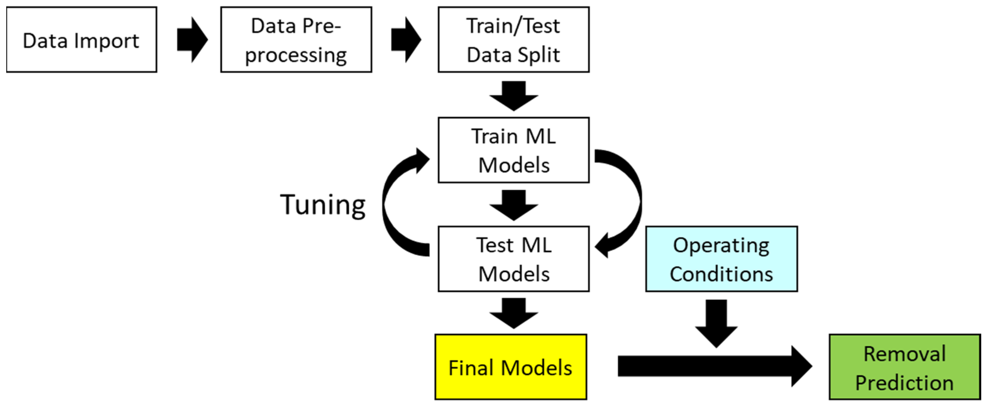
2.2. Development of Data-Based Model (Machine Learning Model)

Two types of machine learning models—regression and classification—were developed using data generated by the physics-based model created in this study. Regression models predict the arsenic removal performance of the EC wastewater system using numerical values, while classification models categorize EC performance into two classes: satisfactory or unsatisfactory removal. A process diagram illustrating the machine learning workflow is shown in Figure 3.

2.2.1. Data Preprocessing

If the feature values used for training the model vary significantly in magnitude, preprocessing is crucial to ensure that they are zero-centered with a unit standard deviation. Machine learning algorithms, particularly distance-based methods, like support vector machines (SVM) and K-nearest neighbors (KNN), perform more effectively when the data are standardized, as they are sensitive to the scale of the features [35,36,37,38]. Standardization prevents features with large numerical values from dominating the learning process, leading to faster convergence and improved model performance. In this study, the dataset was preprocessed using the standard scaling method, as defined in Equation (41), which normalizes the data based on their mean and standard deviation.

$$X_{scaled}={\displaystyle \frac{X-\overline{X}}{\sigma }}$$

(41)

where $\sigma$ denotes the standard deviation of data, $\overline{X}$ is the average value, and $X$ is the feature data.

The dataset is divided into a training set and a testing set, with 75% allocated for model training and the remaining 25% reserved for testing and evaluation. For classification tasks, a stratified split is used to ensure that both the training and testing sets maintain the same class distribution [35,36,37,38]. This approach helps mitigate the impact of class imbalance, resulting in more reliable model development and evaluation.

2.2.2. Machine Learning Algorithms

• K-Nearest Neighbors (KNN)

K-nearest neighbors (KNN) is a distance-based algorithm that classifies or predicts a data point based on its proximity to nearby data points. In classification tasks, KNN assigns a data point to the class that is most frequently represented among its K-nearest neighbors, as determined by the distance formula (Equation (42)). To avoid ties, K should not be an even number or a multiple of the number of classes. For regression tasks, the predicted value is calculated as the average of the K-nearest data points [35,36,37,38].

$$d=\sqrt{{\left(x_2-x_1\right)}^2+{\left(y_2-y_1\right)}^2}$$

(42)

where $x_1$ and $y_1$ are coordinates of data point 1 in a dimensional space, and $x_2$ and $y_2$ denote the coordinates of a surrounding data point.

Support Vector Machine (SVM)

A support vector machine (SVM) is a powerful and versatile machine learning model capable of performing both classification and regression, whether linear or nonlinear. In classification, an SVM constructs a decision boundary, known as a hyperplane, to separate different categories. Predictions for new data points are made based on their position relative to this hyperplane. The algorithm optimizes the placement of the hyperplane by maximizing the margin between it and the closest data points, known as support vectors. The hyperplane is defined by a set of learned weights and an intercept [35,36,37,38].

$$g\left(x\right)=w_0{x}_1+w_1{x}_2+b$$

(43)

where $x_1$ and $x_2$ are the input features, $w_0$ and $w_1$ are the weight vectors, and $b$ is the bias. If the value of g is ≥1, the point specified is in Class 1, and if the value of g is ≤−1, then the point is in Class 2. The goal of an SVM is to find the widest margins that divide the classes.

When used for regression, an SVM adopts a different approach. Instead of maximizing the margin between classes, it seeks to fit as many data points as possible within a defined margin. The algorithm identifies a hyperplane that best captures the majority of the data within these margins, and predictions are made based on the equation of this hyperplane.

• Decision Tree and Random Forest

Decision trees are powerful algorithms capable of capturing complex patterns in data. They are trained using the classification and regression tree (CART) algorithm, which recursively splits the training set into subsets. At each step, the algorithm selects a feature, k, and a threshold, t_k, that yield the purest possible subsets, weighted by their size [35,36,37,38].

$$J\left(k,t_k\right)={\displaystyle \frac{m_{left}}{m}}{G}_{left}+{\displaystyle \frac{m_{right}}{m}}{G}_{right}$$

(44)

where $G_{left/right}$ measures the impurity of the left/right subset, and $m_{left/right}$ is the number of instances in the left/right subset.

Once the training set is split into two subsets, the algorithm applies the same logic recursively to each subset, further dividing them into smaller groups. This process continues until a predefined stopping criterion, such as the maximum tree depth, is reached. The impurity of each split is typically measured using the Gini impurity. Random forest is an ensemble of decision trees, typically trained using the bagging method, where multiple trees are built from different subsets of the training data. The number of samples used for each tree (max. samples) is usually set to match the size of the original training set.

• Lasso and Ridge Regression

Ridge regression is a regularized extension of linear regression, where a regularization term is added to the mean squared error (MSE) in Equation (45). This modification not only helps the model fit the data but also encourages smaller weight values, reducing the risk of overfitting. The regularization term is given by $\alpha \left({‖w‖}_2^2\right)/m$, where w is the vector of feature weights, and ${‖w‖}_2$ represents the ${\mathcal{l}}_2$ norm of the weight vector. Similarly, Lasso regression introduces a regularization term to the cost function, but it employs the ${\mathcal{l}}_1$ norm of the weight vector instead. Hyperparameter α controls the strength of the penalty: when α = 0, the model behaves like standard linear regression, while very large values of α shrink the weight significantly, resulting in a nearly constant model (a horizontal line) [35,36,37,38].

$$J\left(\theta \right)=MSE\left(\theta \right)+{\displaystyle \frac{\alpha }{m}}\sum _{i=1}^n{\theta }_i^2$$

(45)

$$J\left(\theta \right)=MSE\left(\theta \right)+2\alpha \sum _{i=1}^n\left|{\theta }_i\right|$$

(46)

• Logistic Regression

Logistic regression models the relationship between input features and output classes by fitting the data to a sigmoid function, which maps real-valued inputs to a probability range between 0 and 1. A probability threshold, typically set at 50%, is used to classify data points into different categories. The model is trained to optimize the parameters ${\beta }_0$ and ${\beta }_1$ to achieve the most accurate predictions [35,36,37,38].

$$P={\displaystyle \frac{1}{1+e^{-\left({\beta }_0+{\beta }_{1}x\right)}}}$$

(47)

• Voting Ensemble Method

The predictions of multiple models can be combined to improve accuracy by a technique known as the ensemble method. In this approach, models aggregate their results through a voting mechanism. For classification tasks, voting can be either hard or soft. Hard voting assigns equal weight to each model, with the final prediction determined by the majority vote. In contrast, soft voting considers both the predicted class and its probability. Models with higher confidence in their predictions contribute more heavily to the final decision. For regression tasks, ensemble methods, such as the voting regressor, combine individual model predictions by averaging their outputs, leading to a more robust final prediction [35,36,37,38].

2.2.3. Test Methods of Machine Learning Models

• Cross-Validation

The method used for model evaluation is cross-validation. In this process, the dataset is divided into multiple sections, or folds. The model is trained on n − 1 folds and tested on the remaining fold. The result of cross-validation is a set of n accuracy scores, which indicate how well the model generalizes to new data. For classification tasks, stratified cross-validation is employed, where the dataset is split in a way that preserves the same class distribution across all the folds [35,36,37,38].

• Classification

The methods used to evaluate the performance of classification models include the confusion matrix and the receiver operating characteristic (ROC) curve. The confusion matrix is a 2 × 2 table used for binary classification, where the main diagonal represents correct predictions, and the opposite diagonal shows incorrect predictions. The model’s accuracy can be calculated by dividing the number of correct predictions by the total number of predictions.

The ROC curve provides a graphical representation of the model’s performance by plotting the true positive rate (TPR) against the false positive rate (FPR) at various threshold levels. The threshold refers to the probability value at which a prediction is assigned to a specific class. The area under the ROC curve (AUC) is a numerical metric that summarizes the model’s overall performance, with an AUC of 1 indicating a perfect model. As the ROC curve moves inward, the area under the curve decreases, indicating a reduction in the model’s accuracy [35,36,37,38].

• Regression

For a regression model, the performance is evaluated using the R-squared value (coefficient of determination), which can be calculated from the total sum of squares (TSS) and the residual sum of squares (RSS), as shown in Equations (48)–(50) [35,36,37,38].

$$R^2=1-{\displaystyle \frac{RSS}{TSS}}={\displaystyle \frac{\sum _{i=1}^n{\left({\widehat{y}}_i-\overline{y}\right)}^2}{\sum _{i=1}^n{\left(y_i-\overline{y}\right)}^2}}$$

(48)

$$TSS=\sum _{i=1}^n{\left(y_i-\overline{y}\right)}^2$$

(49)

$$RSS=\sum _{i=1}^n{\left(y_i-{\widehat{y}}_i\right)}^2$$

(50)

where $y_i$ is the true label value, ${\widehat{y}}_i$ is the calculated (or predicted) value from the machine learning models, and $\overline{y}$ is the average of the predicted value.

Machine learning models were developed using various open-source modules and libraries in the Python environment, including Scikit-learn for traditional machine learning algorithms, TensorFlow and Keras for neural network algorithms, Pandas for data processing, NumPy for array computations, and Matplotlib for data visualization.

3. Results and Discussion

3.1. Physics-Based Model

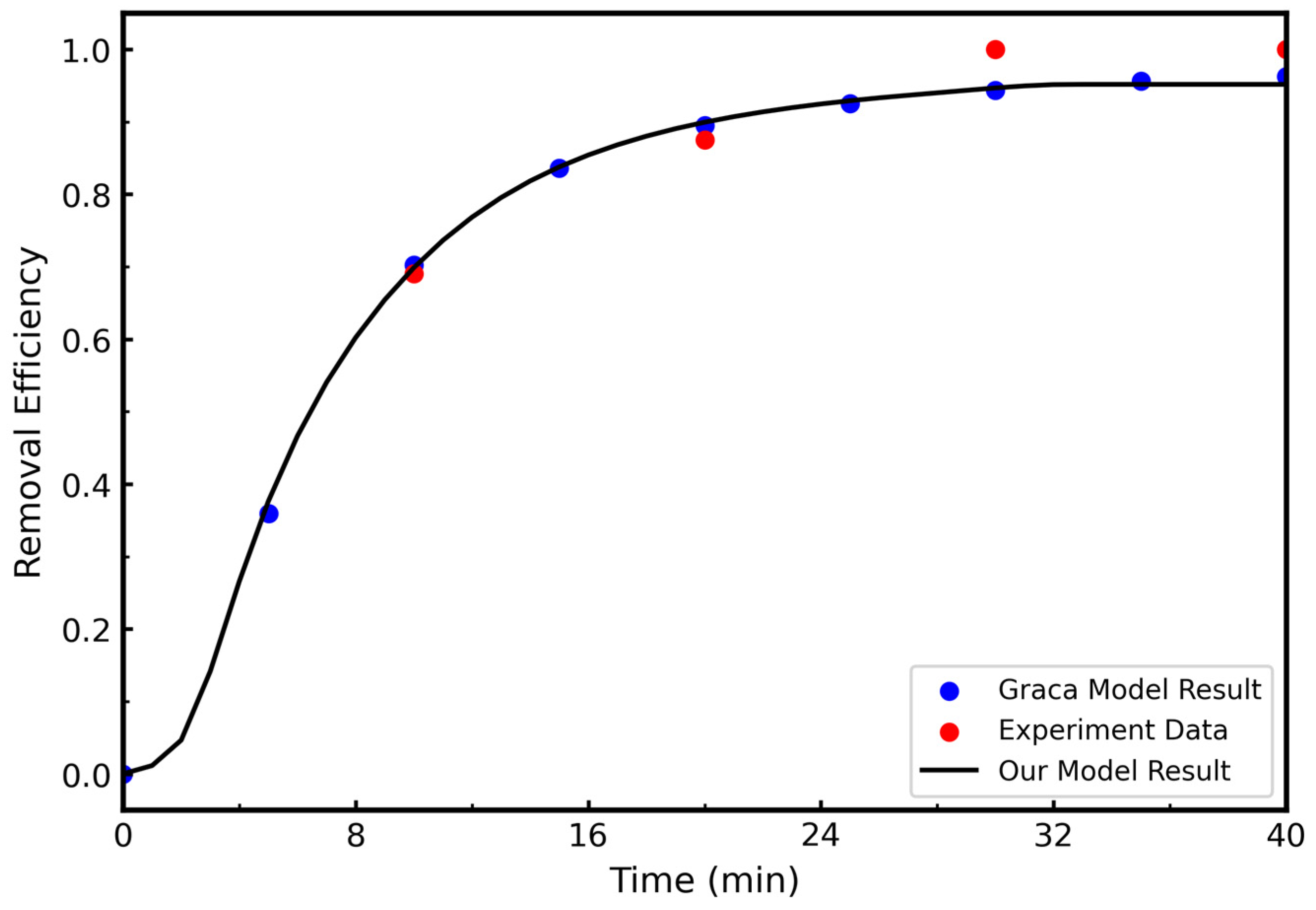
3.1.1. Model Validation

The model predictions were validated using experimental data obtained from ref. [16]. To align with the conditions under which the experimental data were measured, the model was converted to a batch mode (i.e., zero-dimensional model), and the initial arsenic concentration and electrolysis time were set to the same values as those used in the experiment. The surface flux (mol/m²·s) conditions in the model were converted to volumetric generation rates. A better match between the model and experimental data was achieved by adjusting the values of the Langmuir isotherm constants, the separation factor K, and the solid capacity Q in Equation (37). Different values for K and Q were tested to assess their impact on the model’s fit to the experimental data (refer to Appendix A.1). After tuning, the model predictions closely matched the experimental results and model prediction of ref. [16], and a comparison of the model results is shown in Figure 4.

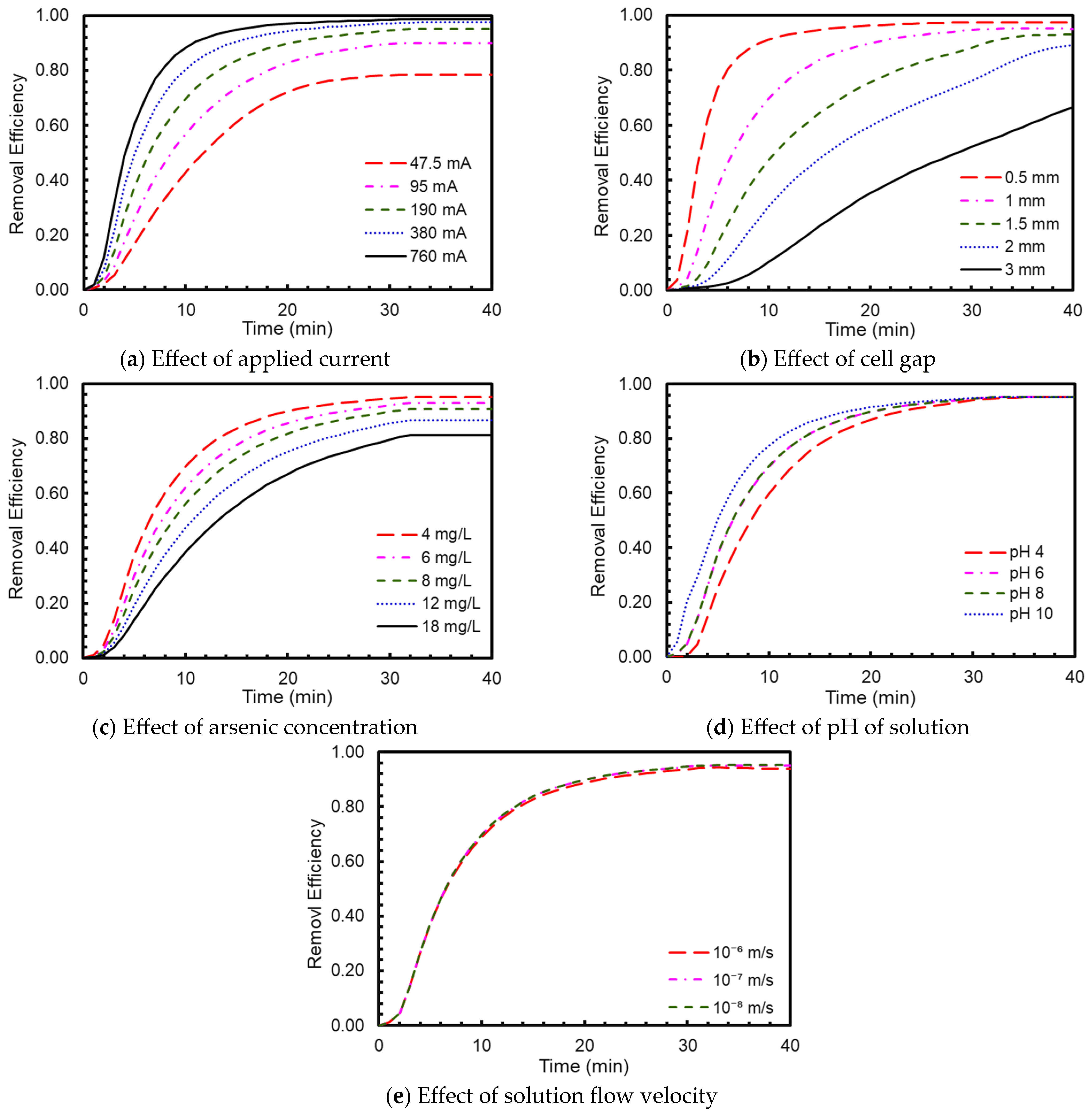
3.1.2. Parametric Study

To generate the data for training the machine learning models, the physics-based model is solved for various combinations of parameters. The resulting data will be used to train the machine learning model, which aims to understand the impact of these parameters and make predictions on the removal percentage. Each parameter is varied individually to isolate its effect on removal performance. A set of baseline values is provided in

Table 3. Baseline parameter values.

Parameter	Value	Units
pH	7	-
Current	190	mA
Cell Gap	1	mm
Initial Arsenic Concentration	4	mg/L
Flow Velocity	$1\times {10}^{-7}$	m/s

, and the parametric study test matrix is presented in

Table 4. Test matrix for parametric study.

Test	Parameter and Range
Parametric Study 1	pH: 4–10
Parametric Study 2	Current: 190 mA, ×0.5, ×0.25, ×2, ×4
Parametric Study 3	Cell gap: 0.5 mm–4mm
Parametric Study 4	Arsenic concentration: 4–20 mg/L
Parametric Study 5	Flow: $1\times {10}^{-6},1\times {10}^{-7},1\times {10}^{-8} \mathrm{m}/\mathrm{s}$

.

It is known that the performance of electrocoagulation (EC) systems is influenced by both system design parameters and processing conditions. Key design parameters include electrode materials (e.g., iron, aluminum, and alloys), electrode configurations (e.g., monopolar, bipolar, parallel, or series), the inter-electrode gap, and reactor types (e.g., batch or continuous-flow reactors). The processing parameters include pH, treatment time, initial pollutant concentration, solution temperature, current intensity, and stirring speed [1,2,3,14].

In this study, we focused on evaluating the effects of the most critical processing parameters on an EC system that is based on aluminum electrodes arranged in a monopolar configuration within a continuous-flow reactor. Additionally, we analyzed the impact of electrode spacing as a key system design parameter. The framework presented in this work is adaptable and can be readily extended to other EC systems with different design configurations of interest.

The effect of current on removal performance is shown in Figure 5a, where the current was varied from 47.5 mA to 700 mA. After 15 min of operation, the initial removal performance was 61%, 74%, 84%, 91%, and 95% for current levels of 47.5, 95, 190, 380, and 760 mA, respectively. The maximum removal rates after 40 min were 78%, 90%, 95%, 98%, and 99% for the same current levels, indicating that current significantly influences the removal rate. This result is attributed to the higher generation rates of Al³⁺ and OH⁻ at higher applied currents, which directly enhance the formation of flocs that adsorb arsenics.

Figure 5b illustrates the effect of the cell gap (i.e., the distance between the two electrodes), where five different gaps—0.5, 1, 1.5, 2, and 3 mm—were compared. After 15 minutes, the removal rates were 95%, 84%, 64%, 48%, and 23% as the cell gap increased from 0.5 mm to 3 mm. The maximum removal rates were 97%, 95%, 93%, 89%, and 67% for the same cell gap conditions, respectively, highlighting the significant impact of cell gap on removal efficiency. The cell gap determines the distance that the ions generated at each electrode must travel to undergo chemical reactions. As the gap increases, the ions take more time to reach the reaction sites, reducing the rate of floc formation and, consequently, lowering arsenic removal efficiency.

The effect of the initial arsenic concentration is shown in Figure 5c. The removal rate decreased as the arsenic concentration increased. After 15 min, the removal rates were 84%, 78%, 73%, 65%, and 56%, while the maximum removal rates were 95%, 93%, 91%, 87min%, and 81% as the arsenic concentration decreased from 18 mg/L to 4 mg/L. As the arsenic concentration increases, more flocs are required to extract them from the polluted solution, which requires more time.

Figure 5d presents the effect of pH on removal efficiency. As the pH increased, the removal rate improved. Notably, when the solution was neutral (pH 6–8), the removal rate remained unaffected. Higher pH levels enhanced arsenic removal, as this is the preferred condition for the agglomeration of flocs.

The effect of flow rate was examined at $1\times {10}^{-6}, 1\times {10}^{-7}, \mathrm{a}\mathrm{n}\mathrm{d} 1\times {10}^{-8} \mathrm{m}/\mathrm{s}$, as illustrated in Figure 5e. While lower flow rates resulted in slightly higher removal efficiency due to longer retention time, the overall effect of the flow rate on removal performance was minimal in the flow rate used in this study. However, the effect of the flow rate is expected to be more significant under higher flow rate conditions, as they impact the retention time of arsenic to be treated.

The arsenic removal behaviors for the various operating conditions agree with the literature [16,17,18,19,20,31], and a detailed analysis of the operating conditions on removal efficiency can be found in our previous research [31].

The parametric studies generated 1150 data points. The data points were organized with respect to the operating conditions and removal percentage. A few data points are shown in

Table 5. Example of test matrix for parametric study.

Time (min)	Current (mA)	${\mathbf{C}}_{\mathbf{0}}\mathbf{(}\mathbf{m}\mathbf{g}\mathbf{/}\mathbf{L}\mathbf{)}$	pH	Flow (m/s)	Cell Gap (mm)	RR (%)
0	190	4	4	$1.0\times {10}^{-7}$	1	0
5	190	4	4	$1.0\times {10}^{-7}$	1	25.3
10	190	4	4	$1.0\times {10}^{-7}$	1	59.7
20	190	4	4	$1.0\times {10}^{-7}$	1	87
30	190	4	4	$1.0\times {10}^{-7}$	1	94

as an example. The dataset should be independent, so duplicates of the baseline were removed.

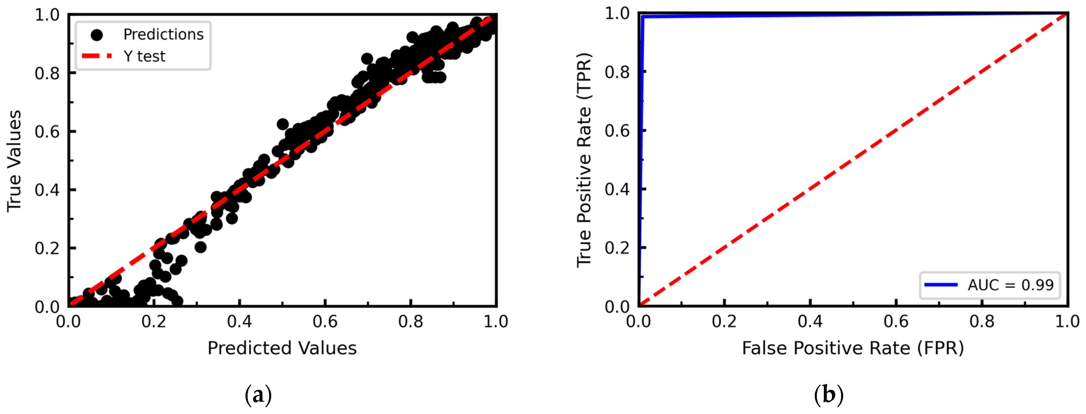
3.2. Data-Based Model

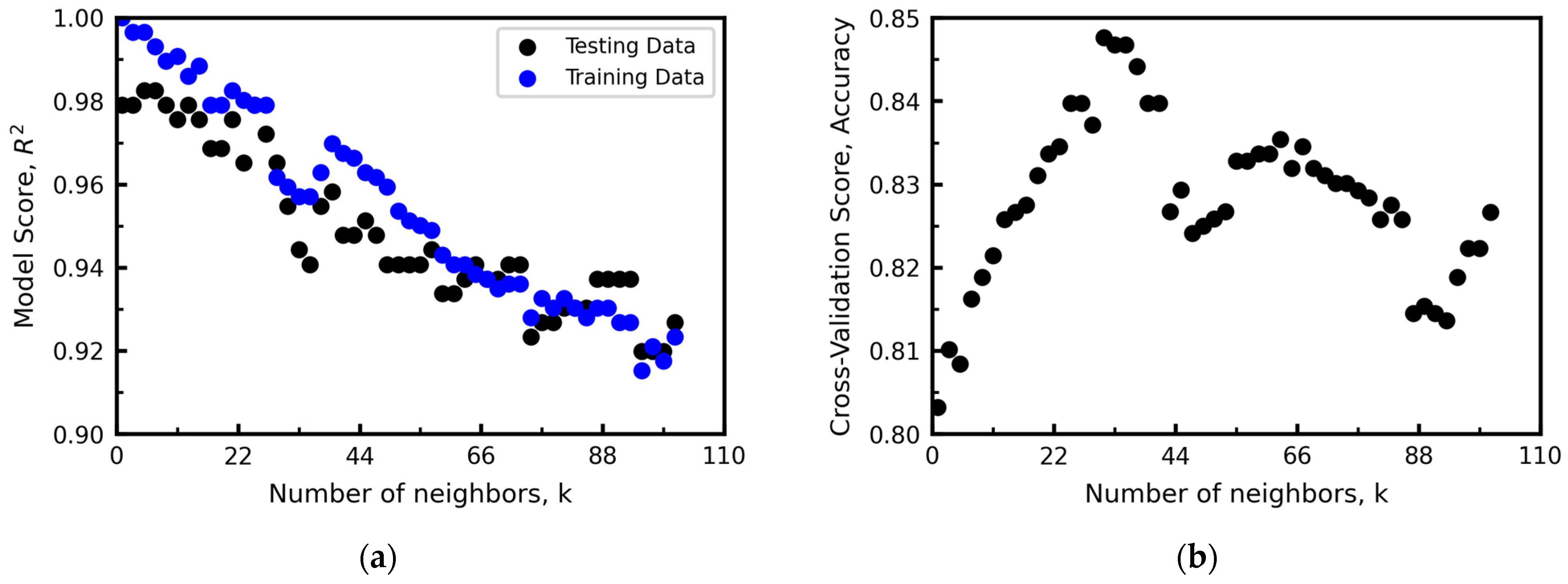
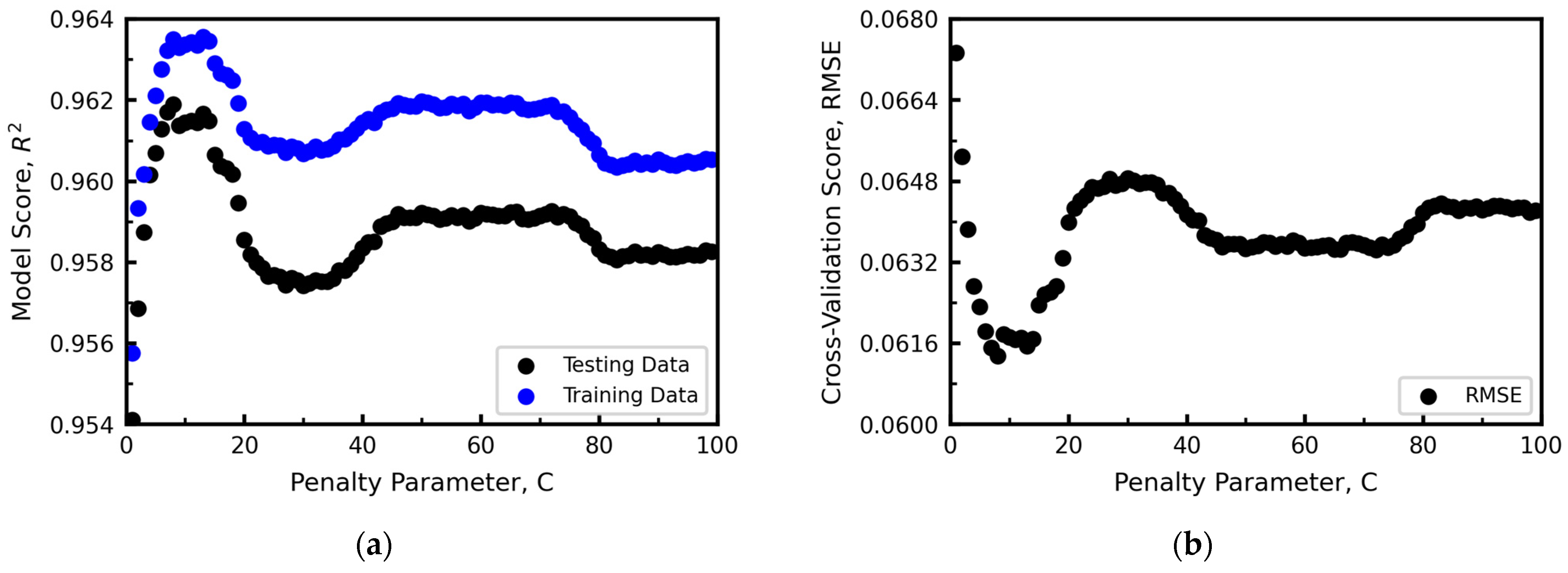
Hyperparameter Optimization

Hyperparameters are parameters that influence the prediction accuracy of machine learning models. These parameters are adjusted during the training process until the prediction accuracy reaches its maximum. Using optimal hyperparameter values is crucial for achieving high predictive performance. In this study, seven machine learning models were employed, each with their own set of hyperparameters. The hyperparameters considered and their effects on the algorithms are summarized in

Table 6. Range of hyperparameter values.

Algorithm	Hyperparameter/Effect	Range Considered
Lasso	α: Strength of penalty	0.01–1
Ridge	α: Strength of penalty	0.01–1
KNN	K: Number of neighbors	1–99 (odd number)
SVM	-Kernel: transform data into linear form -C: high C minimizes error low C maximizes hyperplane margin	RBF, poly, linear1–2000
Decision Tree	-Max. depth: max layers in tree -Min. sample split: minimum points to split node	2–no limit2–10
Random Forest	Number of estimators	1–1000
Voting	Feature weights (regression) Hard/soft (classification)	-

.

The KNN classification algorithm has a key hyperparameter, which is the number of neighbors (K). If K is too small, the model’s predictions will be overly influenced by outliers and will fail to create smooth decision boundaries between classes. On the other hand, if K is too large, the model’s prediction accuracy will decrease. Therefore, the optimal value of K must be determined before applying KNN. Cross-validation accuracy was evaluated for different values of K, with the maximum accuracy achieved at K = 31.

A support vector machine (SVM) uses kernels to transform nonlinear data into a linear form by mapping it into higher-dimensional space. Three types of kernels—linear, polynomial, and radial basis function (RBF)—were used in this study. An SVM also has a regularization parameter, C. As the C value increases, the margin between the hyperplane and the data becomes narrower, improving the classification. However, if C is set too high, the model may overfit by memorizing the training data. Conversely, if C is too low, the hyperplane will have wider margins, allowing for misclassification, which may lead to underfitting. Therefore, selecting the appropriate kernel and C value is critical. In this study, the prediction accuracy of the SVM was compared with respect to these hyperparameters to identify the optimal configuration (refer to Appendix A.2).

For the decision tree classification algorithm, the key hyperparameters are max. depth and min. sample split. The best performance was achieved using the default parameter values in the Scikit-learn library. The optimal parameters for the machine learning algorithms used in this study are summarized in

Table 7. Optimal hyperparameter values for regression.

Algorithm (Regression)	Hyperparameter	Result
Lasso	α	0.01
Ridge	α	1
KNN	K	3
SVM	Kernel, C	RBF, C = 8
Decision Tree	Max. depth, min. sample split	Default (a)
Random Forest	Number of estimates	100
Voting	Feature weights	Equal

^(a) The default value of the model in the Scikit-learn library was used.

for the regression models and

Table 8. Optimal hyperparameter values for classification.

Algorithm (Classification)	Hyperparameter	Result
KNN	K	31
SVM	Kernel, C	RBF, C = 1100
Decision Tree	Max. depth, min. sample split	Default (b)
Random Forest	Number of estimators	Default (c)
Voting	Hard/soft	Soft

^{(b), (c)} The default value of the model in the Scikit-learn library was used.

for the classification models.

Voting ensemble was used as the final algorithm to further advance the prediction accuracy calculated from all the individual algorithms. The mean squared error is 0.0007, and the R² value is 0.99 for the regression model, and for classification, the F1 score is 0.98, and the AUC is 0.99, as shown in Figure 6.

3.3. Generation of Processing Map

The trained machine learning models were used to generate two processing maps, namely, a regression map and a classification map, which illustrate the arsenic removal behavior across a range of operating conditions in electrocoagulation (EC). These maps serve as essential guidelines for operating or designing a continuous EC system. The regression map was converted into a classification map using a 90% removal rate as the decision threshold. Removal rates above this threshold are classified as acceptable (represented by the blue region in the map), while rates below this threshold are classified as unacceptable (indicated by the red region in the map). This classification map can be customized by adjusting the threshold value to meet the desired removal rates for specific systems.

3.3.1. Processing Map: Effect of Cell Gap

The arsenic removal performance is shown in Figure 7a, where varying color intensities represent the removal rate. As time increases and the cell gap decreases, the removal performance improves. This is because more flocs are generated as the operation time increases, and as the cell gap decreases, ions can more easily pass through the electrodes, enhancing the necessary reactions. This map helps us to understand the combined effect of cell gap and operation time on the removal rate and provides valuable operational guidelines. The plot can also be converted into a classification map, offering clear operational conditions to achieve the desired removal rate. Figure 7b was generated using a 90% removal rate as the decision threshold and clearly shows the cell gap and operating conditions required to reach the blue region. As the figure illustrates, achieving the target removal rate is impossible if the cell gap exceeds 1.9 mm, and even with the smallest cell gap of 0.5 mm, at least 10 min of operation is required to reach the desired removal rate.

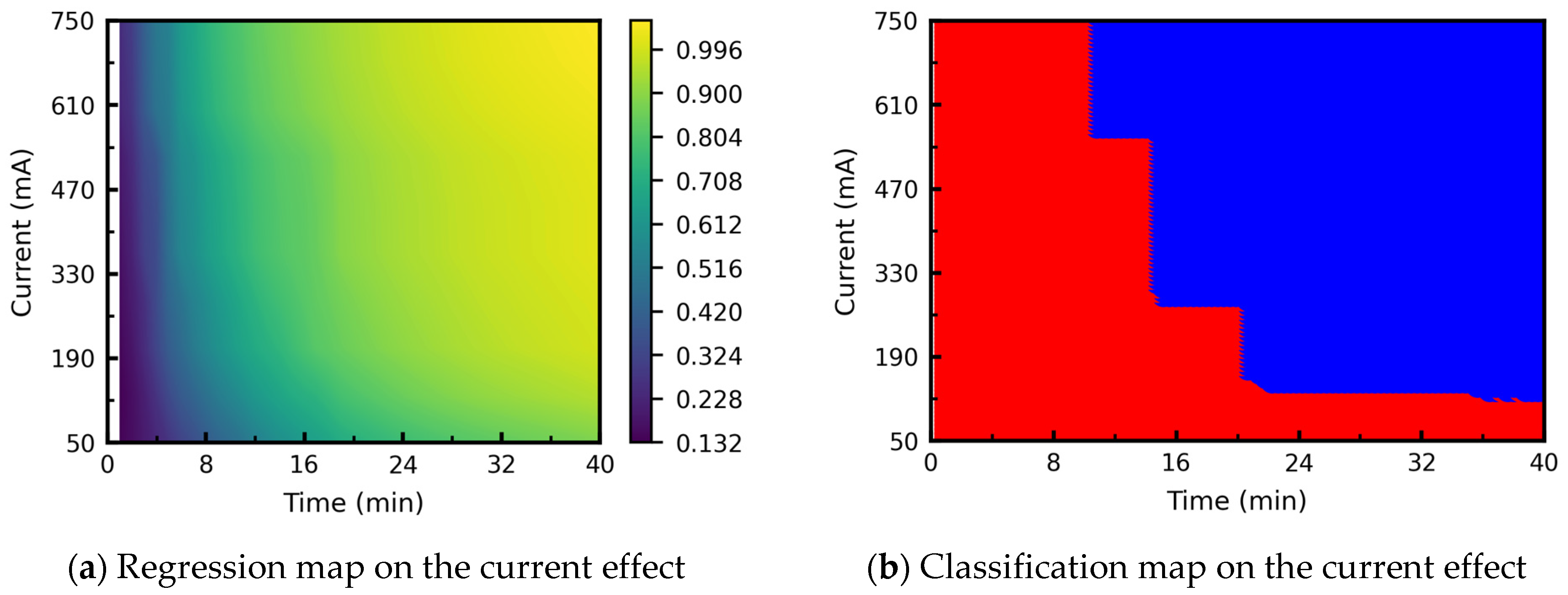
3.3.2. Processing Map: Effect of Current

One of the key operating conditions for EC is the current intensity, which requires guidelines to select appropriate values. A regression map was developed to show removal rates across a range of currents from 50 to 750 mA over a 40 min operation, as shown in Figure 8a. As the applied current and operation time increase, the removal rate also increases due to the enhanced floc generation resulting from a higher current and longer operation time. These effects are clearly depicted in the classification map, which was created using a 90% removal rate as the decision threshold. As shown in Figure 8b, if the current is below 170 mA, achieving an acceptable removal rate is impossible. Additionally, even with the highest applied current of 750 mA, at least 12 min are required to reach the desired removal rate. This map provides clear guidance on how to design and operate the EC system.

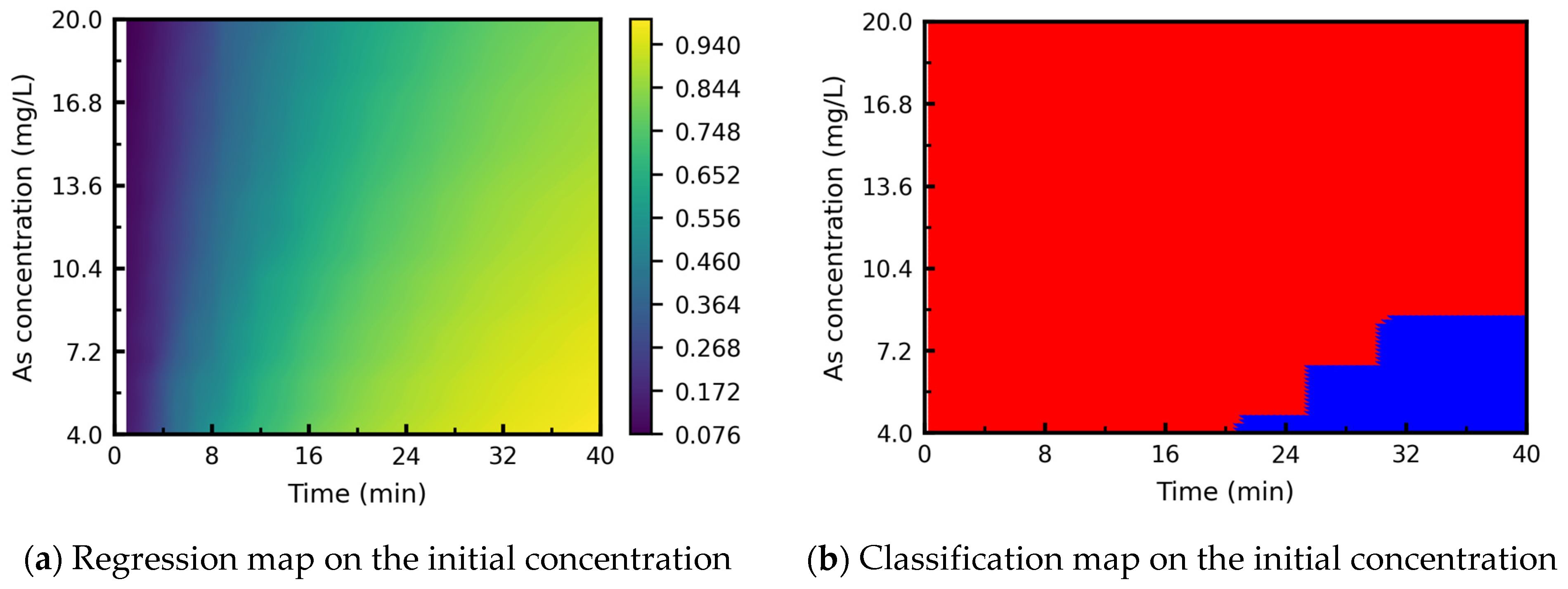
3.3.3. Processing Map: Effect of Initial Arsenic Concentration

EC operation needs to be adjusted based on factors such as the degree of pollution in the wastewater. The effect of the initial arsenic concentration on the removal rate is shown in two operation maps—regression and classification maps—across a concentration range from 4 to 20 mg/L. The removal efficiency increased as the initial concentration decreased and the operation time increased. This effect is clearly depicted in the classification map, which was created using a 90% removal rate as the decision threshold. As shown in Figure 9b, if the initial concentration exceeds 8.8 mg/L, the desired removal rate cannot be achieved within 40 min. Even at the lowest concentration of 4 mg/L, at least 20 min of operation time is required. These processing maps were generated for the operating conditions utilized in this study but they can be customized for different operating scenarios to provide tailored operating guidelines.

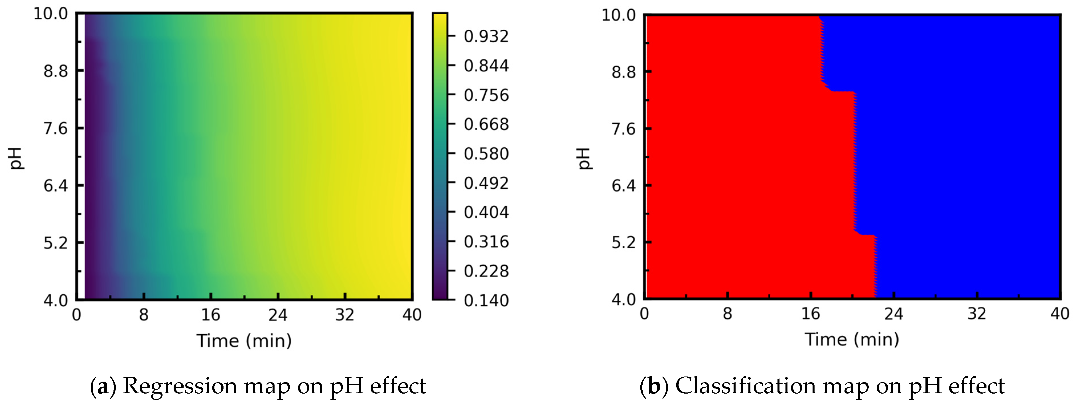
3.3.4. Processing Map: Effect of pH

Wastewater often contains various impurities that can influence its pH levels. Therefore, understanding the effect of pH on EC performance is crucial for determining optimal operating conditions for the EC system. The removal performance is presented in the processing maps in Figure 10, which show the relationship between pH and operation time. Higher pH values (i.e., basic conditions) result in a slight increase in removal performance, while lower pH values (i.e., acidic conditions) lead to a slight decrease in performance. This effect is further illustrated in the classification map in Figure 10b, where approximately 20 min of operation is required under neutral conditions, and 16 min are sufficient for a basic condition at pH 10, while 22 min are required for an acidic condition at 4.

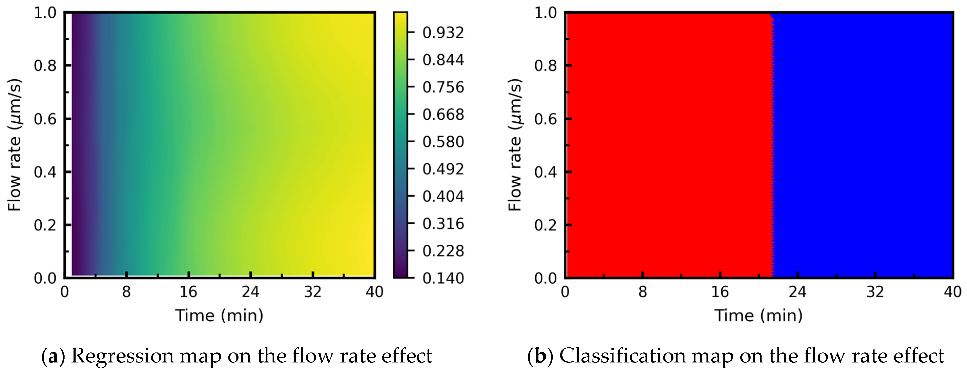
3.3.5. Processing Map: Effect of Flow Rate

This system is a continuous EC system in which wastewater circulates between the EC cell and a storage tank. The flow rate of this circulation is another key operating condition that needs to be determined. Figure 11 illustrates the operation map showing the effect of flow rate on the removal rate. The removal rate did not change significantly, likely due to the low flow rates used in this study, ranging from 1 × 10⁻⁶ to 1 × 10⁻⁸ m/s. These values were chosen due to convergence issues in the computational simulations, which were constrained by the limited resources available. However, this research lays the groundwork for future studies in this field. The classification map indicates that the removal rate is primarily influenced by the operation time. If the flow rate is too high, the species may be swept out of the cell before they have a chance to interact. It is anticipated that at very high flow velocities, the flow could break up the flocs, leading to reduced performance. Investigating the effect of flow rate at higher velocities will be the focus of our future work.

4. Conclusions

In this study, a more realistic two-dimensional unsteady-state mathematical model was developed for a continuous electrocoagulation (EC) system. The model incorporates comprehensive multiphysics phenomena, including electrochemical and chemical reactions, ionic mass transport via diffusion and convection, physical adsorption of pollutants onto flocs, and the recirculation effect between the external tank and the EC cell. The simulation results provide valuable insights into the impact of various operating parameters on the pollutant removal efficiency of the EC system.

After validation, the developed physics-based model was used to generate data on removal efficiency under a wide range of operating conditions, including applied current, inter-electrode gap, initial arsenic concentration, flow rate, and pH. These data were then used to train seven machine learning (ML) algorithms: Lasso, Ridge, K-nearest neighbors (KNN), support vector machine (SVM), decision tree, random forest, and voting (soft/hard). To improve prediction accuracy, rigorous hyperparameter tuning was performed, and the models were further enhanced through ensemble learning. The validated model was also employed to generate processing maps at a 90% removal rate as the decision threshold, which correlates the removal efficiency with the key operating parameters.

This study revealed that multiple operational parameters significantly influence the removal rate. For the cell gap, achieving the target removal rate is not possible when it exceeds 1.9 mm, and even at the minimum gap of 0.5 mm, at least 10 min of operation are necessary. Regarding the applied current, values below 170 mA are insufficient to attain an acceptable removal rate, while even at the maximum current of 750 mA, a minimum of 12 min is still required. In terms of the initial arsenic concentration, concentrations above 8.8 mg/L prevent reaching the desired removal rate within 40 min, and even at the lowest tested concentration of 4 mg/L, a minimum of 20 min is needed. The solution pH also plays a role, with approximately 20 min required under neutral conditions, 16 min at pH 10, and 22 min at pH 4. Lastly, the flow rate had minimal impact on removal efficiency due to the low flow rates used, but it is anticipated that excessively high flow velocities could sweep reactive species out of the cell prematurely or break up flocs, thereby reducing treatment performance.

This study presents a comprehensive framework for analyzing electrocoagulation (EC) systems by integrating physics-based and data-driven modeling approaches. The proposed methodology provides valuable insights for system developers aiming to understand EC fundamentals, while also serving as a practical guide for system operators to optimize EC performance. Although this study focuses on arsenic-contaminated wastewater due to the availability of experimental data, the framework can be applied to the analysis of various types of wastewater.

While the current model effectively simulates the EC system, several opportunities for future enhancement remain. On the physics-based modeling side, future efforts should consider incorporating the formation and evolution of floc structures and their role in arsenic adsorption, electrode passivation phenomena, the influence of ionic migration on species transport, and the effects of turbulence promoters to enhance mixing. On the data-driven modeling side, exploring more advanced neural network architectures, such as hybrid models combining convolutional neural networks (CNNs) and recurrent neural networks (RNNs), could further improve predictive accuracy.

References

1. Patel, S.K.; Shukla, S.C.; Natarajan, B.R.; Asaithambi, P.; Dwivedi, H.K.; Sharma, A.; Singh, D.; Nasim, M.; Raghuvanshi, S.; Sharma, D.; et al. State of the art review for industrial wastewater treatment by electrocoagulation process: Mechanism, cost and sludge analysis. Desalination Water Treat. 2025, 321, 100915. [Google Scholar] [CrossRef]
2. Jo, S.; Kadam, R.; Jang, H.; Seo, D.; Park, J. Recent Advances in Wastewater Electrocoagulation Technologies: Beyond Chemical Coagulation. Energies 2024, 17, 5863. [Google Scholar] [CrossRef]
3. Mao, Y.; Zhao, Y.; Cotterill, S. Examining Current and Future Applications of Electrocoagulation in Wastewater Treatment. Water 2023, 15, 1455. [Google Scholar] [CrossRef]
4. Silva, J.F.A.; Graça, N.S.; Ribeiro, A.M.; Rodrigues, A.E. Electrocoagulation process for the removal of co-existent fluoride, arsenic and iron from contaminated drinking water. Sep. Purif. Technol. 2018, 197, 237–243. [Google Scholar] [CrossRef]
5. Fajardo, A.S.; Rodrigues, R.F.; Martins, R.C.; Castro, L.M.; Quinta-Ferreira, R.M. Phenolic wastewaters treatment by electrocoagulation process using Zn anode. Chem. Eng. J. 2015, 275, 331–341. [Google Scholar] [CrossRef]
6. İrdemez, Ş.; Demircioğlu, N.; Yıldız, Y.Ş.; Bingül, Z. The effects of current density and phosphate concentration on phosphate removal from wastewater by electrocoagulation using aluminum and iron plate electrodes. Sep. Purif. Technol. 2006, 52, 218–223. [Google Scholar] [CrossRef]
7. Grich, N.B.; Attour, A.; Mostefa, M.L.P.; Tlili, M.; Lapicque, F. Fluoride removal from water by electrocoagulation with aluminium electrodes: Effect of the water quality. Desalination Water Treat. 2019, 144, 145–155. [Google Scholar] [CrossRef]
8. Nidheesh, P.V.; Singh, T.S.A. Arsenic removal by electrocoagulation process: Recent trends and removal mechanism. Chemosphere 2017, 181, 418–432. [Google Scholar] [CrossRef]
9. Amrose, S.; Gadgil, A.; Srinivasan, V.; Kowolik, K.; Muller, M.; Huang, J.; Kostecki, R. Arsenic removal from groundwater using iron electrocoagulation: Effect of charge dosage rate. J. Environ. Sci. Health Part A 2013, 48, 1019–1030. [Google Scholar] [CrossRef]
10. Gomes, J.A.G.; Daida, P.; Kesmez, M.; Weir, M.; Moreno, H.; Parga, J.R.; Irwin, G.; McWhinney, H.; Grady, T.; Peterson, E.; et al. Arsenic removal by electrocoagulation using combined Al–Fe electrode system and characterization of products. J. Hazard. Mater. 2007, 139, 220–231. [Google Scholar] [CrossRef]
11. Lai, C.L.; Lin, S.H. Electrocoagulation of chemical mechanical polishing (CMP) wastewater from semiconductor fabrication. Chem. Eng. J. 2003, 95, 205–211. [Google Scholar] [CrossRef]
12. Wang, C.-T.; Chou, W.-L.; Chen, L.-S.; Chang, S.-Y. Silica particles settling characteristics and removal performances of oxide chemical mechanical polishing wastewater treated by electrocoagulation technology. J. Hazard. Mater. 2009, 161, 344–350. [Google Scholar] [CrossRef] [PubMed]
13. Chen, G. Electrochemical technologies in wastewater treatment. Sep. Purif. Technol. 2004, 38, 11–41. [Google Scholar] [CrossRef]
14. Moussa, D.T.; El-Naas, M.H.; Nasser, M.; Al-Marri, M.J. A comprehensive review of electrocoagulation for water treatment: Potentials and challenges. J. Environ. Manag. 2017, 186, 24–41. [Google Scholar] [CrossRef]
15. Magnisali, E.; Yan, Q.; Vayenas, D.V. Electrocoagulation as a revived wastewater treatment method-practical approaches: A review. J. Chem. Technol. Biotechnol. 2022, 97, 9–25. [Google Scholar] [CrossRef]
16. Graça, N.S.; Ribeiro, A.M.; Rodrigues, A.E. Modeling the electrocoagulation process for the treatment of contaminated water. Chem. Eng. Sci. 2019, 197, 379–385. [Google Scholar] [CrossRef]
17. Matteson, M.J.; Dobson, R.L.; Glenn, R.W.; Kukunoor, N.S.; Waits, W.H.; Clayfield, E.J. Electrocoagulation and separation of aqueous suspensions of ultrafine particles. Colloids Surf. A: Physicochem. Eng. Asp. 1995, 104, 101–109. [Google Scholar] [CrossRef]
18. Khemis, M.; Leclerc, J.-P.; Tanguy, G.; Valentin, G.; Lapicque, F. Treatment of industrial liquid wastes by electrocoagulation: Experimental investigations and an overall interpretation model. Chem. Eng. Sci. 2006, 61, 3602–3609. [Google Scholar] [CrossRef]
19. Lacasa, E.; Cañizares, P.; Sáez, C.; Martínez, F.; Rodrigo, M.A. Modelling and cost evaluation of electro-coagulation processes for the removal of anions from water. Sep. Purif. Technol. 2013, 107, 219–227. [Google Scholar] [CrossRef]
20. Carmona, M.; Khemis, M.; Leclerc, J.-P.; Lapicque, F. A simple model to predict the removal of oil suspensions from water using the electrocoagulation technique. Chem. Eng. Sci. 2006, 61, 1237–1246. [Google Scholar] [CrossRef]
21. Lu, J.; Li, Y.; Yin, M.; Ma, X.; Lin, S. Removing heavy metal ions with continuous aluminum electrocoagulation: A study on back mixing and utilization rate of electro-generated Al ions. Chem. Eng. J. 2015, 267, 86–92. [Google Scholar] [CrossRef]
22. Song, P.; Song, Q.; Yang, Z.; Zeng, G.; Xu, H.; Li, X.; Xiong, W. Numerical simulation and exploration of electrocoagulation process for arsenic and antimony removal: Electric field, flow field, and mass transfer studies. J. Environ. Manag. 2018, 228, 336–345. [Google Scholar] [CrossRef]
23. Dubrawski, K.L.; Du, C.; Mohseni, M. General Potential-Current Model and Validation for Electrocoagulation. Electrochim. Acta 2014, 129, 187–195. [Google Scholar] [CrossRef]
24. Chen, X.; Chen, G.; Yue, P.L. Investigation on the electrolysis voltage of electrocoagulation. Chem. Eng. Sci. 2002, 57, 2449–2455. [Google Scholar] [CrossRef]
25. Balasubramanian, N.; Kojima, T.; Srinivasakannan, C. Arsenic removal through electrocoagulation: Kinetic and statistical modeling. Chem. Eng. J. 2009, 155, 76–82. [Google Scholar] [CrossRef]
26. Amani-Ghadim, A.R.; Aber, S.; Olad, A.; Ashassi-Sorkhabi, H. Optimization of electrocoagulation process for removal of an azo dye using response surface methodology and investigation on the occurrence of destructive side reactions. Chem. Eng. Process. Process Intensif. 2013, 64, 68–78. [Google Scholar] [CrossRef]
27. Garg, K.K.; Prasad, B. Development of Box Behnken design for treatment of terephthalic acid wastewater by electrocoagulation process: Optimization of process and analysis of sludge. J. Environ. Chem. Eng. 2016, 4, 178–190. [Google Scholar] [CrossRef]
28. Akoulih, M.; Tigani, S.; Byoud, F.; Rharib, M.E.; Saadane, R.; Pierre, S.; Chehri, A.; Ghachtouli, S.E. Electrocoagulation-based AZO DYE (P4R) Removal Rate Prediction Model using Deep Learning. Procedia Comput. Sci. 2024, 236, 51–58. [Google Scholar] [CrossRef]
29. Bhagawati, P.B.; Kiran Kumar, H.S.; Lokeshappa, B.; Malekdar, F.; Sapote, S.; Adeogun, A.I.; Chapi, S.; Goswami, L.; Mirkhalafi, S.; Sillanpää, M. Prediction of electrocoagulation treatment of tannery wastewater using multiple linear regression based ANN: Comparative study on plane and punched electrodes. Desalination Water Treat. 2024, 319, 100530. [Google Scholar] [CrossRef]
30. Shirkoohi, M.G.; Tyagi, R.D.; Vanrolleghem, P.A.; Drogui, P. A comparison of artificial intelligence models for predicting phosphate removal efficiency from wastewater using the electrocoagulation process. Digit. Chem. Eng. 2022, 4, 100043. [Google Scholar] [CrossRef]
31. Dey, S.; Adejinle, A.; Cho, K.T. Modeling Study of Aluminum-Based Electrocoagulation System for Wastewater Treatment. J. Environ. Eng. 2024, 150, 04023099. [Google Scholar] [CrossRef]
32. Newman, J.S.; Thomas-Alyea, K.E. Electrochemical Systems, 3rd ed.; J. Wiley: Hoboken, NJ, USA, 2004. [Google Scholar]
33. Kundu, P.K.; Cohen, I.M.; Dowling, D.R.; Tryggvason, G. Fluid Mechanics, 6th ed.; Elsevier: Amsterdam, The Netherlands, 2016. [Google Scholar]
34. Xiao, F.; Zhang, B.; Lee, C. Effects of low temperature on aluminum(III) hydrolysis: Theoretical and experimental studies. J. Environ. Sci. 2008, 20, 907–914. [Google Scholar] [CrossRef] [PubMed]
35. Murphy, K.P. Machine Learning—A Probabilistic Perspective; MIT Press: Cambridge, MA, USA, 2014. [Google Scholar]
36. Goodfellow, I.; Bengio, Y.; Courville, A. Deep Learning; The MIT Press: Cambridge, MA, USA, 2016. [Google Scholar]
37. Bishop, C.M.; Bishop, H. Deep Learning: Foundations and Concepts; Springer: Cham, Switzerland, 2024. [Google Scholar]
38. Lee, W.-M. Python Machine Learning; John Wiley and Sons: Indianapolis, IN, USA, 2019. [Google Scholar]
Figure 1. A typical electrocoagulation system.
Sustainability 17 04604 g001
Figure 2. Diagram of continuous flow electrocoagulation (EC) test system. (1) External mixing tank, (2) pump, (3) tubing, (4) inlet of EC cell, (5) anode electrode, (6) cathode electrode, (7) outlet of EC cell, and white arrows indicate the flow direction of wastewater.
Sustainability 17 04604 g002
Figure 3. Overall procedure for training machine learning models and generating predictions.
Sustainability 17 04604 g003
Figure 4. Validation of model prediction with experimental data and model prediction from ref. [16].
Sustainability 17 04604 g004
Figure 5. Effect of operation conditions on arsenic removal efficiency.
Sustainability 17 04604 g005
Figure 6. Prediction performance of final ensemble model for regression and classification. (a) Comparison of true and predicted values for regression. (b) Receiver operating characteristic (ROC) curve for classification.
Sustainability 17 04604 g006
Figure 7. Arsenic removal plot for the effects of operating time and cell gap. The color bar in Figure (a) represents the arsenic removal rate from wastewater, and in Figure (b), the blue region denotes acceptable removal rates, whereas the red region indicates unacceptable levels.
Sustainability 17 04604 g007
Figure 8. Arsenic removal plot for the effects of operating time and current. The color bar in Figure (a) represents the arsenic removal rate from wastewater, and in Figure (b), the blue region denotes acceptable removal rates, whereas the red region indicates unacceptable levels.
Sustainability 17 04604 g008
Figure 9. Arsenic removal for the effects of operating time and arsenic concentration. The color bar in Figure (a) represents the arsenic removal rate from wastewater, and in Figure (b), the blue region denotes acceptable removal rates, whereas the red region indicates unacceptable levels.
Sustainability 17 04604 g009
Figure 10. Arsenic removal plot for the effects of operating time and pH. The color bar in Figure (a) represents the arsenic removal rate from wastewater, and in Figure (b), the blue region denotes acceptable removal rates, whereas the red region indicates unacceptable levels.
Sustainability 17 04604 g010
Figure 11. Arsenic removal plot for the effects of operating time and flow. The color bar in Figure (a) represents the arsenic removal rate from wastewater, and in Figure (b), the blue region denotes acceptable removal rates, whereas the red region indicates unacceptable levels.
Sustainability 17 04604 g011