A State-Specific Approach for Visualizing Overburdened Communities: Lessons from the Connecticut Environmental Justice Screening Tool 2.0

Abstract

While multiple federal screening tools have previously been developed for mapping communities facing environmental injustice and health disparities, many states across the United States have seen value in developing state-specific screening tools. This article provides an overview of a recent addition to the list of state screening tools, the Connecticut Environmental Justice Screening Tool (CT EJScreen). CT EJScreen identifies communities disproportionately affected by environmental and socioeconomic burdens at the census tract level. The tool integrates geospatial data on potential pollution sources, exposures, health sensitivities, and socioeconomic factors to produce a cumulative Environmental Justice Index. This article describes the development process of the tool, its methodological framework, the multi-pronged public engagement during the development process, preliminary correlation analyses, lessons learned, and recommendations for future iterations. Spearman correlation and Principal Component Analysis were applied to assess variable relationships and guide indicator refinement. Stakeholder engagement with Connecticut’s environmental justice communities ensured that the tool reflects both quantitative data and lived experiences. CT EJScreen provides important information for policy implementation covering areas such as funding, public health issues, and permitting. The CT EJScreen process might serve as a useful template for other states looking to devise state-specific adjunct screening systems.

1. Introduction

Online mapping tools have been commonly used to identify and visualize environmental justice (EJ) concerns over the last decade. The Environmental Protection Agency’s (EPA) nationwide EJScreen, released to the public in 2015 [1], along with similar tools from the Centers for Disease Control and Prevention [2] and the Council on Environmental Quality [3], highlights communities impacted by environmental and socioeconomic burdens [4,5]. These tools can serve as initial screening mechanisms, directing resources to areas in need [6].

While federal tools provide broad insights, they often fail to capture state-specific environmental and demographic conditions [7] and can be vulnerable to changes in federal administrations. In response, states such as California, Colorado, Michigan, and Washington have developed their own EJ screening tools [8,9,10,11]. State-specific tools address federal shortcomings, ensuring screening aligns with local policy needs and community priorities [12].

Connecticut has a longstanding history of environmental justice efforts, particularly in Bridgeport, New Haven, and Hartford. Industrialization throughout the 20th century led to disproportionate pollution and hazardous waste exposure in marginalized communities. The 1993 Environmental Equity Policy marked the state’s first acknowledgment of environmental injustice, but a lack of standardized, high-resolution data hindered its implementation.

In 2021, Governor Lamont’s Executive Order No. 21-3 established the Connecticut Equity and Environmental Justice Advisory Council (CEEJAC) to guide pollution reduction and climate resiliency efforts. Despite progress, policymakers lacked a centralized, Connecticut-specific screening tool to identify at-risk communities and guide interventions. In response, the Connecticut Institute for Resilience and Climate Adaptation (CIRCA) and the Connecticut Department of Energy and Environmental Protection (CT DEEP) developed the Connecticut Environmental Justice Screening Tool (CT EJScreen). The first public version, CT EJScreen version 2.0 [13], was released in August 2023 after an iterative development process incorporating advisory committee input, community forums, and public comments.

The goal of this study is to document the development of a state-level cumulative impact screening tool that is applied to support environmental justice efforts. Specifically, we answer the research question of how the Connecticut Environmental Justice Screening Tool (CT EJScreen) identifies and addresses areas of disproportionate environmental and health burdens and what its potential impact is on shaping future environmental justice policies and practices in Connecticut. This study presents CT EJScreen as a first screening roadmap for identifying and addressing environmental and health disparities in Connecticut. We showcase its development, methodology, and statistical analyses to demonstrate its effectiveness in capturing disparities tied to environmental justice. Additionally, we assess its applicability to policy, determine its limitations, and propose recommendations for developing the next iteration, CT EJScreen 3.0. This case study emphasizes the necessity for state-level environmental justice tools amidst federal uncertainty and offers a model to ensure such tools are scientifically robust, policy-relevant, and community-driven.

2. Materials and Methods

The development of CT EJScreen 2.0 was led by CIRCA at the University of Connecticut. CIRCA’s involvement went beyond combining data; it integrated stakeholder participation, advisory feedback, and review of methods, thereby ensuring that CT EJScreen is scientifically valid and community-based. Contrary to conventional exposure analyses that respond to single hazards, CT EJScreen considers the cumulative impacts of multiple stressors on public health. CT EJScreen shares core methodological features with leading environmental justice tools such as EPA’s EJScreen [14], CalEnviroScreen [4,9], and Washington’s Environmental Health Disparities Map [6,11], but it also incorporates key distinctions that reflect Connecticut’s specific environmental and social landscape. CT EJScreen adopts a cumulative impact framework that combines environmental burdens with health sensitivity and socioeconomic stressors into a multi-layered index like CalEnviroScreen and Washington’s tool. CT EJScreen relies on census tract-level spatial resolution, similar to 76% of reviewed EJ tools [15]. Some federal data (e.g., ACS, EPA datasets) are used as supplements when local data are lacking, but emphasis was given to Connecticut-specific inputs (e.g., DPH-provided health indicators, land use datasets), consistent with best practices identified for effective state tools.

Unlike some national tools that primarily highlight pollution exposures (e.g., EPA’s EJScreen), CT EJScreen also integrates social determinants like food insecurity, education, and mental health, aligning more closely with CalEnviroScreen’s and Colorado EnviroScreen’s [8] comprehensive vulnerability models. CT EJScreen also includes an iterative stakeholder engagement process to reflect the emerging issues with the tool design. For more details on all the indicator calculations and the whole project, please refer to the technical report [13].

2.1. Literature Review and Indicator Selection

Initially, the indicators were chosen based on an analysis of national- and state-level environmental justice screening tools through literature review and their community relevance by the Connecticut Governor’s Council on Climate Change’s (GC3) Equity and Environmental Justice Workgroup [16]. This workgroup report [16] prioritized indicators that represent aspects of environmental justice, have scientific evidence from other state tools to link environmental or health burdens, were of sufficient quality, minimized redundancy, and have replicability. The indicators were further refined throughout the project by incorporating the feedback from the State Data Advisory Committee (SDAC), the Connecticut Department of Public Health (CT DPH), and the Connecticut Department of Energy and Environmental Protection (CT DEEP) to enhance their relevance, data quality, geographic specificity, consistency, and policy applicability throughout developing different versions of the tool [13]. Key selection criteria included statewide data availability, public accessibility, compatibility with census tract-level resolution, data quality, and relevance to environmental and health vulnerabilities observed in Connecticut. We also considered redundancy, spatial granularity, and cumulative impacts. The data processing steps followed are as follows:

• Dataset Collection: Data were collected on potential pollution exposure, potential pollution sources, socioeconomic factors, and health sensitivities (Table 1). CT EJScreen has 48 indicators that provide a broader range of information. Its sub-categories allow flexible analyses of overlapping burdens [15].
• Geospatial Assignment: Raw data were assigned to census tracts to balance geographic accuracy with statistical stability. Buffers were used around pollution source point locations to account for the impact of dispersion [13]. A standard 1 km (km) buffer radius was used, with the assumption that communities within this distance are most likely to be affected [4,9]. This 1 km radius was subdivided into four distance-based zones—250 m, 500 m, 750 m, and 1000 m—with decreasing weights (1, 0.5, 0.25, and 0.1, respectively) to reflect attenuated impacts over distance. Locations beyond 1 km were assigned a weight of zero. For pollution sources associated with odors or air quality complaints (e.g., landfills, incinerators), double buffer distances up to 2 km were applied with proportionally scaled weights (1, 0.5, 0.25, and 0.1) to reflect their broader community impact [4,9,17]. The weighted values were summed per census tract spatial intersection and then converted into percentiles and decile ranks. This structured approach ensures consistency in evaluating relative exposure potential across tracts while reflecting the spatial decay of pollution impact. Other indicator categories did not need buffering. A step-by-step calculation of each indicator is detailed in [13].
• Percentile Ranking and Normalization: Raw values were converted to percentiles (0–100) to enable comparisons and then normalized to a 0–10 scale for comparability. The linear normalization is performed by

$${Rank}_n={\displaystyle \frac{\left(P_n-P_{min}\right)}{\left(P_{max}-P_{min}\right)}}+\left(Decile Range\right),$$

(1)

where $P_n$ is the original percentile for a particular tract n; $P_{min}$ is the minimum value among all the tracts, which is 0 for percentiles; $P_{max}$ is the maximum value among all the tracts; and $Decile Range$ is the difference between the maximum and minimum values of the new range, which is 10 − 0 = 10, in this case. A 0 percentile and rank often mean there are no data available below that tract. An example of a step-by-step calculation is given in Appendix A.

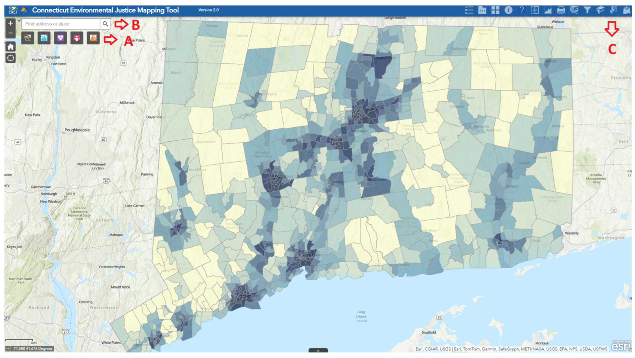
• Map Development: Processed indicators were integrated into an online Geographic Information System (GIS) web format, using the ArcGIS Online Web Application (https://www.arcgis.com/index.html, accessed 11 May 2025).

Table 1. List of indicators used in CT EJScreen version 2.0. Please refer to [13] for the methodology of each calculation. (Accessed date for all sources: 25 March 2025).

Indicator Category	Indicator	Source
Potential Pollution Sources	Brownfield Sites	CT DEEP Hazardous Waste Inventory 2021, Brownfields
	EPCRA Tier II/Facilities Managing Chemicals	EPCRA Tier II Locations, CT DEEP-CT SERC, 2021
	Lead Paint Risk in Housing	2017–2021 American Community Survey 5-Year Estimates
	Impervious Surfaces	2021 MRLC Impervious Land Cover
	Incinerators/Resource Recovery Facilities	CT Resource Recovery Facilities, 2020
	Landfills	Active Landfills 2020 and Affecting Facilities 2021
	Municipal Transfer Stations	2020 CT DEEP Municipal Waste Disposal Data
	Potentially Contaminated Sites	2021 CT DEEP Hazard Waste Inventory, Remediation Department
	Proximity to Superfund Sites	2022 EPA CERCLIS
	Recycling Processing Facilities/Materials Recovery Facilities	2018 CT DEEP Recycling Processing Facilities
	Significant Environmental Hazards/Proximity to Facilities with Highly Toxic Substances	2023 Significant Environmental Hazards, CT DEEP
	Underground Storage Tanks (USTs)—Active Facilities	2021 CT Gov Active Underground Storage Tank (UST) Facilities
	Wastewater Discharge	2019 Risk-Screening Environmental Indicators (RSEI) modeled results by EPA’s Office of Pollution Prevention and Toxics on 15 March 2021
Potential Pollution Exposure	Diesel Particulate Matter (PM) Emissions	EPA EJSCREEN 2022, National Emissions Inventory, EPA Hazardous Air Pollutants 2017
	EPA Air Toxins Assessment Respiratory Hazard Index	Air Toxics Data Update, EPA EJSCREEN 2022
	EPA Air Toxins Assessment Cancer Risk	Air Toxics Data Update, EPA EJSCREEN 2022
	Facilities Releasing Toxins	TRI Form R and A 2021 CT DEEP and U.S. Environmental Protection Agency and CT Department of Energy and Environmental Protection
	Minor Facilities with Permit-Limited Emissions Potential	2023 Section 22a-174 33a and 33b facilities CT DEEP Bureau of Air Management Title V permits—CT DEEP Bureau of Air Management
	Noise	U.S. Department of Transportation, Bureau of Transportation Statistics, National Transportation Noise Map, 2018
	Ozone	NASA Socioeconomic Data and Applications Center [18],
	Particulate Matter (PM) 2.5	Atmospheric Composition Analysis, Washington University in St. Louis [19]
	Permitted Major Air Pollution Sources	2021 Title V permits—CT DEEP Bureau of Air Management Title V permits—CT DEEP Bureau of Air Management
	Permitted Minor Air Pollution Sources/Equipment/Processes	2021 New Source Review Permits—CT DEEP Bureau of Air Management
	Traffic Density	2020 Traffic Monitoring Annual Average Daily Traffic Report, CT Department of Transportation
	Urban Heat Index	2003–2018 UHI Earth Engine Data Catalog
Health Sensitivity	Asthma Emergency Department Visits	2015–2019 CT DPH—Connecticut Inpatient Hospitalization and Emergency Department Visit Dataset
	Chronic Obstructive Pulmonary Disease (COPD) Emergency Department Visits	2013–2017 Connecticut State Department of Public Health COPD Health Viewer
	Childhood Elevated Blood Lead Levels	2016–2020 Connecticut State Department of Public Health Childhood Lead Poisoning Surveillance Report
	Coronary Heart Disease	2021 PLACES—Center for Disease Control and Prevention
	Depression Rates	2020 PLACES—Center for Disease Control and Prevention
	Diabetes	2021 PLACES—Center for Disease Control and Prevention
	Low Birthweight Rate of Infants	2016–2020 CT DPH Health Statistics and Surveillance Section, Births Dataset
	Poor Mental Health	2021 PLACES—Center for Disease Control and Prevention
Socioeconomic Factors	Educational Attainment	2017–2021 American Community Survey 5-Year Data
	Elderly Population
	Housing Burden
	Food Insecurity
	Linguistic Isolation
	Median Income
	Mobile Homes
	Multi-Unit Housing
	Population without Health Insurance
	Race/Ethnicity
	Poverty
	Population with Disability
	Population under 5 Years Old
	Rent–Ownership Ratio
	Single-Parent Household
	Lack of Tree Canopy	2021 MRLC Tree Canopy Cover
	Energy Burden	2020 Low-Income Energy Affordability Data (LEAD)
	Unemployment	2023 Connecticut Department of Labor Current Monthly Data

Table 1. List of indicators used in CT EJScreen version 2.0. Please refer to [13] for the methodology of each calculation. (Accessed date for all sources: 25 March 2025).

Indicator Category	Indicator	Source
Potential Pollution Sources	Brownfield Sites	CT DEEP Hazardous Waste Inventory 2021, Brownfields
	EPCRA Tier II/Facilities Managing Chemicals	EPCRA Tier II Locations, CT DEEP-CT SERC, 2021
	Lead Paint Risk in Housing	2017–2021 American Community Survey 5-Year Estimates
	Impervious Surfaces	2021 MRLC Impervious Land Cover
	Incinerators/Resource Recovery Facilities	CT Resource Recovery Facilities, 2020
	Landfills	Active Landfills 2020 and Affecting Facilities 2021
	Municipal Transfer Stations	2020 CT DEEP Municipal Waste Disposal Data
	Potentially Contaminated Sites	2021 CT DEEP Hazard Waste Inventory, Remediation Department
	Proximity to Superfund Sites	2022 EPA CERCLIS
	Recycling Processing Facilities/Materials Recovery Facilities	2018 CT DEEP Recycling Processing Facilities
	Significant Environmental Hazards/Proximity to Facilities with Highly Toxic Substances	2023 Significant Environmental Hazards, CT DEEP
	Underground Storage Tanks (USTs)—Active Facilities	2021 CT Gov Active Underground Storage Tank (UST) Facilities
	Wastewater Discharge	2019 Risk-Screening Environmental Indicators (RSEI) modeled results by EPA’s Office of Pollution Prevention and Toxics on 15 March 2021
Potential Pollution Exposure	Diesel Particulate Matter (PM) Emissions	EPA EJSCREEN 2022, National Emissions Inventory, EPA Hazardous Air Pollutants 2017
	EPA Air Toxins Assessment Respiratory Hazard Index	Air Toxics Data Update, EPA EJSCREEN 2022
	EPA Air Toxins Assessment Cancer Risk	Air Toxics Data Update, EPA EJSCREEN 2022
	Facilities Releasing Toxins	TRI Form R and A 2021 CT DEEP and U.S. Environmental Protection Agency and CT Department of Energy and Environmental Protection
	Minor Facilities with Permit-Limited Emissions Potential	2023 Section 22a-174 33a and 33b facilities CT DEEP Bureau of Air Management Title V permits—CT DEEP Bureau of Air Management
	Noise	U.S. Department of Transportation, Bureau of Transportation Statistics, National Transportation Noise Map, 2018
	Ozone	NASA Socioeconomic Data and Applications Center [18],
	Particulate Matter (PM) 2.5	Atmospheric Composition Analysis, Washington University in St. Louis [19]
	Permitted Major Air Pollution Sources	2021 Title V permits—CT DEEP Bureau of Air Management Title V permits—CT DEEP Bureau of Air Management
	Permitted Minor Air Pollution Sources/Equipment/Processes	2021 New Source Review Permits—CT DEEP Bureau of Air Management
	Traffic Density	2020 Traffic Monitoring Annual Average Daily Traffic Report, CT Department of Transportation
	Urban Heat Index	2003–2018 UHI Earth Engine Data Catalog
Health Sensitivity	Asthma Emergency Department Visits	2015–2019 CT DPH—Connecticut Inpatient Hospitalization and Emergency Department Visit Dataset
	Chronic Obstructive Pulmonary Disease (COPD) Emergency Department Visits	2013–2017 Connecticut State Department of Public Health COPD Health Viewer
	Childhood Elevated Blood Lead Levels	2016–2020 Connecticut State Department of Public Health Childhood Lead Poisoning Surveillance Report
	Coronary Heart Disease	2021 PLACES—Center for Disease Control and Prevention
	Depression Rates	2020 PLACES—Center for Disease Control and Prevention
	Diabetes	2021 PLACES—Center for Disease Control and Prevention
	Low Birthweight Rate of Infants	2016–2020 CT DPH Health Statistics and Surveillance Section, Births Dataset
	Poor Mental Health	2021 PLACES—Center for Disease Control and Prevention
Socioeconomic Factors	Educational Attainment	2017–2021 American Community Survey 5-Year Data
	Elderly Population
	Housing Burden
	Food Insecurity
	Linguistic Isolation
	Median Income
	Mobile Homes
	Multi-Unit Housing
	Population without Health Insurance
	Race/Ethnicity
	Poverty
	Population with Disability
	Population under 5 Years Old
	Rent–Ownership Ratio
	Single-Parent Household
	Lack of Tree Canopy	2021 MRLC Tree Canopy Cover
	Energy Burden	2020 Low-Income Energy Affordability Data (LEAD)
	Unemployment	2023 Connecticut Department of Labor Current Monthly Data

2.2. Developing Cumulative Impact Model

CT EJScreen employs a cumulative impact framework [4,20,21,22,23,24,25] to quantify environmental and social burdens at the census tract level. The cumulative impact model accounts for the combined effects of multiple environmental and social stressors. This methodology follows the principle [26]:

Risk = Threat × Vulnerability

(2)

The threat in the model represents the community’s pollution burden, while vulnerability comes from the community’s characteristics. Equation (2) transforms into

Environmental Justice Index (EJ_Index) = Pollution Burden × Sensitive Population

(3)

Pollution Burden (Threat) consists of pollution sources and pollution exposures, and Sensitive Populations (Vulnerability) includes health sensitivity and socioeconomic factors in Equation (3).

$$Pollution Burden= {\displaystyle \frac{0.5\times average \left(Potential Pollution Sources\right)+average (Potential Pollution Exposure) }{1.5}}$$

(4)

$$Sensitive Population={\displaystyle \frac{average\left(Socieoeconomic Factors\right)+average(Health Sensitivity)}{2}}$$

(5)

The model generates seven cumulative indices, which are then combined into an overall Environmental Justice Index (EJ_Index). Within the composite category of Pollution Burden were two sub-categories, pollution sources and pollution exposures, with pollution sources weighted at 50% of pollution exposures to reflect actual exposure risks, with pollution exposures weighted more heavily than pollution sources [9] (Equation (4)). The composite category Sensitive Population consisted of two combined sub-categories: socioeconomic factors and health sensitivity (Equation (5)). All four sub-categories (potential pollution sources, potential pollution exposures, socioeconomic factors, and health sensitivity) were compiled from a series of individual indicator layers representing different pollution or sensitivity factors. Each indicator (represented in Table 1) has equal weight under each sub-category due to not having enough scientific evidence to apply a weighting between indicators [27]. Indicator averages represent the related sub-category index. The step-by-step index calculation is given in Appendix A.

CT EJScreen version 2.0 calculates layers at the census tract level. Smaller geographic units, such as block groups, were deemed less reliable due to higher variability in small population estimates. Similarly to indicator calculations, all indices are calculated by combining their normalized scores, converting them to percentiles, and then creating a new normalized ranking of 0–10 across census tracts. By assigning numerical values and ranks to each census tract, the tool displays the communities’ relative standing. The darker areas on the map indicate a higher potential impact of the EJ.

2.3. Stakeholder Engagement

We recognized that data alone cannot fully capture environmental injustices. To actively integrate diverse stakeholder participation into the tool’s development, we held public forums, advisory committees, and public feedback mechanisms. The tool reflected both quantitative data and lived experiences via these engagement activities. Feedback from engagement sessions directly informed improvements throughout the eight versions developed until reaching version 2.0, such as simplifying the fact sheet layout, expanding map layer options, translating the tool into Spanish, and incorporating contextually relevant layers like energy burden and odor pollution indicators. The Mapping Tool Advisory Committee (MTAC) further guided the design by recommending clearer legends, more intuitive color scales, and a more accessible layout for turning map layers on and off. Additionally, CIRCA created visual tutorials and revised web content to clarify complex methodological concepts, a direct response to confusion expressed in forums. Participants’ input also led to the decision to develop a standalone website for the tool, improving its accessibility and visibility for communities statewide.

2.3.1. Public Forums

We partnered with local community-based organizations to hold the tool evaluation sessions in Bridgeport, Hartford, Groton, Waterbury, and New Haven, all of which are recognized as environmental justice communities by the State of Connecticut. Partner organizations included youth programs, social services organizations, a neighborhood revitalization zone community group, and a local health department, leading to a diverse array of participants. Three evaluation sessions were held in English, and two were held in Spanish; accompanying materials were provided in both languages. Participants tested a beta version of the tool, provided feedback on usability and accuracy, and voiced their local concerns. Financial compensation was provided to community partners through stipends and to participants through gift cards for their time and input.

2.3.2. Advisory Committees

To include the perspectives and different points of view of state agencies and data providers in the developing process of CT EJScreen, advisory committees were developed to provide their technical expertise, guidance, and insights. These committees played a crucial role in refining indicator selection, ensuring data accuracy as well as the tool’s compatibility with Connecticut’s environmental justice policies and regulatory frameworks.

• State Data Advisory Committee (SDAC): Representatives from state agencies, research institutions, and non-governmental organizations provided technical expertise on data sources, indicator inclusion, and methodological consistency. These included the Office of Policy & Management, Yale Center on Climate Change & Health, DataHaven, Department of Economic and Community Development, Department of Transportation, Department of Public Health, Department of Emergency Services and Public Protection, the Clean Air Association of the Northeast States, and the Connecticut Data Collaborative. This diverse coalition provided technical expertise, data insights, and policy alignment of the tool.
• Mapping Tool Advisory Committee (MTAC): This committee comprised community-based organizations and individuals with lived experience reflecting how environmental burdens manifest in local communities. MTAC members included representatives from Operation Fuel and Groundwork Bridgeport, as well as community members with lived environmental justice experiences from Bridgeport, Windsor, and New Haven. Operation Fuel provides energy assistance to low-income households, while Groundwork Bridgeport focuses on environmental sustainability and urban revitalization. This committee was established through a competitive grant application process in Fall 2022, after which all applications were reviewed by the Grant Advisory Committee and six applicants were selected. Participants were financially compensated through monthly stipends for the duration of the project to ensure broad representation and equitable participation.
• Grant Advisory Committee: This committee played a key role in selecting applicants for the MTAC and supporting broader grant-making efforts. Experts from state and federal agencies, universities, and advocacy organizations guided funding mechanisms to support environmental justice initiatives. Additionally, CIRCA meets with this committee to administer Climate and Equity Grants, which provide funding to nonprofit organizations working on environmental justice, climate resilience, and community engagement initiatives. These grant programs further align with CT EJScreen’s mission by directing resources to organizations that serve historically overburdened communities, reinforcing the tool’s role in equitable decision-making and capacity-building across the state.

2.3.3. Public Feedback

The tool was released for public review through a webinar, and feedback was collected via online surveys during the comment periods. Over 200 responses were reviewed for refinements and openly addressed.

2.4. WebMap Features and User Resources

CT EJScreen is hosted on ArcGIS Online Web AppBuilder to provide convenient access to environmental justice data (Figure 1) and is available at https://connecticut-environmental-justice.circa.uconn.edu/ (accessed on 10 May 2025). This interactive, user-friendly interface allows users to explore spatial disparities in pollution burden and community sensitivities. Users can navigate the map by entering addresses or adjusting it manually. The tool includes various widgets for contextual analysis, overlaying context layers, changing base maps, and filtering tracts by ranking, reporting, charting, and comparing layers. The processed indicators and indices are hosted in ArcGIS Hub to ensure accessibility.

CT EJScreen is also available in Spanish to enhance usability and inclusivity. We developed a comprehensive set of resources in both English and Spanish, including fact sheets, a WebMap, and user guides consisting of two-page mini-guides, widget descriptions, and step-by-step written and video tutorials.

The platform provides extensive resources on potential applications, ideas for action, and supplementary resources to support community advocacy and policy efforts. All the supporting materials can be accessed through the website given supporting information can be downloaded at https://connecticut-environmental-justice.circa.uconn.edu/ (accessed on 12 May 2025). A high school lesson plan designed for second-language speakers, along with an FAQ section and a glossary, is provided so that the tool is accessible to diverse audiences.

3. Results

There are a total of 879 tracts defined in Connecticut based on the 2020 Census. Based on the normalized decile rank categorization ranging from 0 to 10, 85 tracts are categorized as the lowest (rank between 0 and 0.99), and the number of tracts was relatively consistent across intermediate ranks, ranging from 9.7% to 10.1% of tracts from 1 to 9. Only five tracts, or about 0.6% of the total, are between the ranks 9.01 and 10. This distribution reinforces the importance of targeting interventions not only at the very highest-scoring tracts but also at the broader range of highly impacted areas (ranks 6–10) comprising about 40% of tracts.

We also compared how many highly impacted tracts identified by CT_EJScreen were also identified by block groups qualified as EJ communities by CT State Statute 22a-20a [28] CT State Statute 22a-20a defines EJ block groups as any block groups in which 30% or more of the population lives below 200% of the federal poverty level. There are 753 EJ block groups identified, and about 75% of them fall within CT_EJScreen rank values of 6 to 10. This demonstrates strong alignment between statutory socioeconomic criteria and the tool’s cumulative burden assessments.

Spearman correlation and Principal Component Analysis (PCA) were applied to understand the relationship between the indicators and indices. Spearman correlation was used to assess the strength and direction of pairwise relationships between individual indicators, revealing how different stressors may co-occur across census tracts. However, it does not capture the multivariate dataset structure or indicate whether there can be a more concise set of indicators that can represent the full data. PCA was performed to identify dominant patterns and evaluate whether a smaller subset of variables could represent the same cumulative indices. PCA also informs potential weighting schemes for future iterations of the tool. Together, these methods support the refinement of indicator selection and weighting strategies for future versions of CT EJScreen. In this article, dataset names used within CT EJScreen are presented in the Courier font (e.g., Impervious_Surfaces) to distinguish them from general references to the same concept.

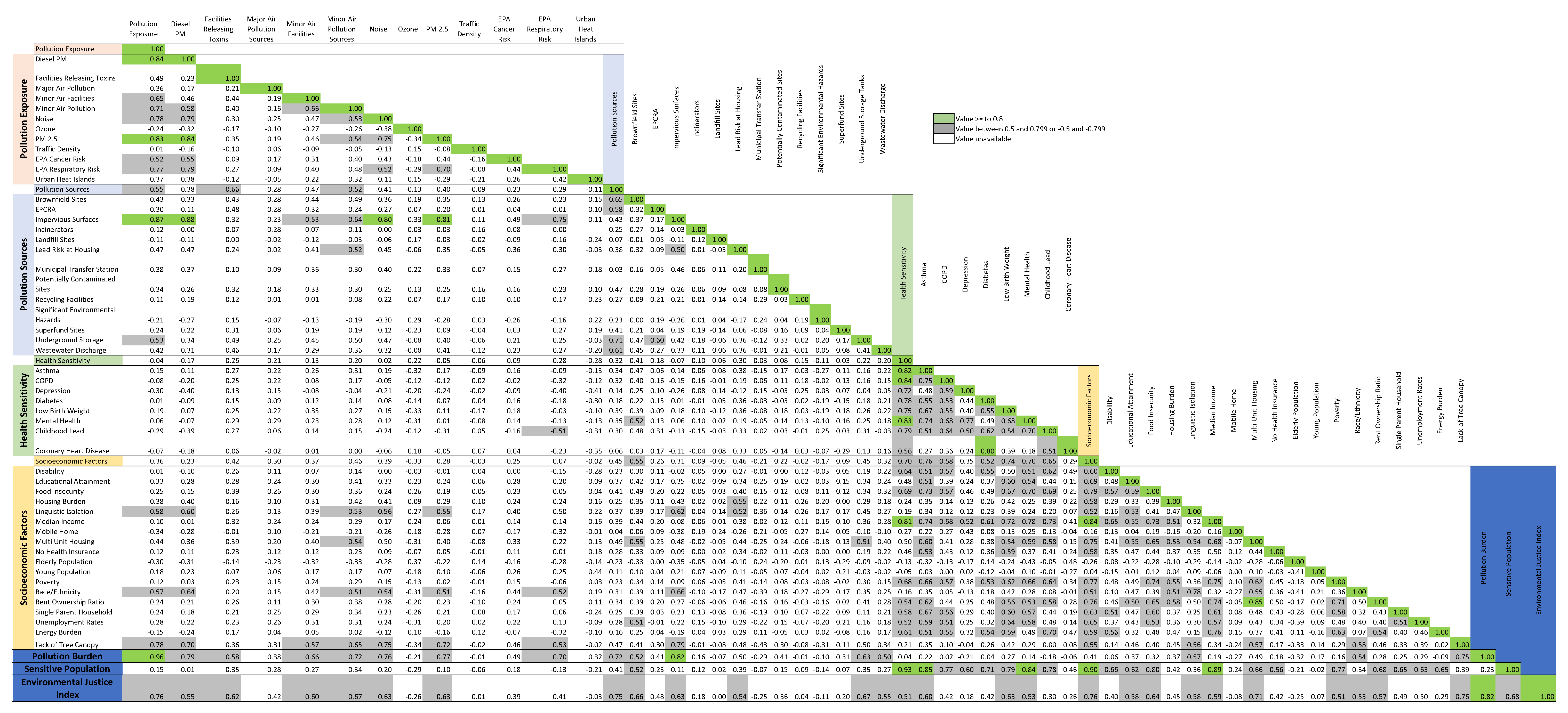
3.1. Spearman Analysis

A Spearman correlation test was used to identify statistically significant strengths and directional relationships between indicator values in the EJ_Index. Spearman correlation was useful for identifying statistically significant relationships between indicators and understanding how different environmental, health, and socioeconomic factors interact within CT EJScreen. Spearman detected patterns of co-occurrence and showed where the overlapping content of two indicators occurred. Similarly to [6]’s approach, a correlation coefficient above 0.8 was considered a strong correlation, while values between 0.5 and 0.8 indicated moderate correlations, and any coefficient lower than 0.5 was considered a low correlation (Figure 2).

3.1.1. Spearman Analysis of Potential Pollution Exposure

PM2.5_Emission and Diesel_PM_Emissions are strongly correlated (p = 0.84), suggesting they frequently co-occur in high-exposure areas. Both indicators also showed strong correlations with the Pollution_Exposure_Index (p = 0.83 and p = 0.84, respectively), confirming their dominant contribution to cumulative pollution burdens. Notable moderate correlations highlight high-traffic areas and industrial sources as overlapping contributors to environmental burdens. For example, Diesel_PM_Emissions is moderately correlated with Noise (p = 0.71) and Minor_Air_Pollution_Sources (p = 0.65), suggesting shared origins in transportation or industrial activity. Similarly, clusters of industrial activity appear where urban noise and air pollution co-occur, as seen in the correlations between Minor_Air_Pollution_Sources and Minor_Air_Pollution_Facilities (p = 0.60), and between EPA_AirToxinAssessment_Respiratory_Risk and both Noise (p = 0.59) and PM2.5 (p = 0.61). There is some association between cancer and respiratory risk indices and air pollution (EPA_AirToxinAssessment_Cancer_Risk and Diesel_PM_Emissions (p = 0.63), EPA_AirToxinAssessment_Respiratory_Risk and Diesel_PM_Emissions (p = 0.68)), which raises concerns over the long-term health impacts of air pollution.

3.1.2. Spearman Analysis of Potential Pollution Sources

Impervious_Surfaces demonstrated strong correlations with multiple pollution sources, including Diesel_PM_Emissions (p = 0.88), PM2.5 (p = 0.81), and Noise (p = 0.80), indicating that densely built areas coincide with air and noise pollution. Other moderate correlations highlight the relationship between industrial activity and pollution clustering (such as those between Impervious_Surfaces and Minor_Air_Pollution_Facilities (p = 0.61) and between Impervious_Surfaces and Minor_Air_Pollution_Sources (p = 0.62)). Further correlations indicate overlaps between industrial contamination sources, such as between EPCRA_Facilities and Underground_Storage_Tanks (p = 0.60), reflecting the co-location of hazardous chemical storage and industrial facilities. The correlation between Lead_Risk_in_Housing and Impervious_Surfaces (p = 0.58) suggests the possibility of legacy pollution in high-density urban areas.

3.1.3. Spearman Analysis of Health Sensitivity

Health_Sensitivity_Index was highly correlated with Asthma_ER_Visits (p = 0.82), COPD_Rates (p = 0.84), and Poor_Mental_Health (p = 0.83), indicating chronic illnesses and mental health as health stressors. Diabetes and Coronary_Heart_Disease exhibited a strong correlation (p = 0.80), reinforcing the need to consider co-occurring health conditions in cumulative health burdens.

3.1.4. Spearman Analysis of Socioeconomic Factors

Multi-Unit_Housing and Rent_Ownership_Ratio strongly correlated (p = 0.85), demonstrating rental-heavy communities. The Socioeconomic_Factors_Index was highly correlated with Median_Income (p = 0.84), further indicating the role of economic disparity.

3.1.5. Cross-Category Correlations of Spearman Analysis

Several cross-category correlations reveal how pollution exposure aligns with social and environmental disparities. Notably, Diesel_PM_Emissions correlated with Linguistic_Isolation (p = 0.58), Race (p = 0.63), and Lack_of_Tree_Canopy (p = 0.55), suggesting that diverse racial groups and linguistically isolated populations may be disproportionately exposed to air pollution. Similarly, Impervious_Surfaces correlated with Linguistic_Isolation (p = 0.58), Race (p = 0.64), and Lack_of_Tree_Canopy (p = 0.57), reflecting patterns of environmental inequities in urbanized areas. Brownfield_Sites were linked to socioeconomic hardship (Multi-Unit_Housing (p = 0.57) and Unemployment (p = 0.59)), emphasizing the connection between industrial legacies and economic disadvantages.

3.1.6. Key Findings of Spearman Analysis

The Environmental Justice Index (EJ_Index) was closely correlated with the Pollution_Burden_Index (p = 0.82). This strong connection shows that pollution significantly contributes to environmental injustice. The results of the Spearman correlation analysis provide important insights for understanding the drivers of environmental injustice in Connecticut.

Pollution primarily contributes to overall environmental justice concerns, especially in urbanized areas with high impervious surface coverage. Brownfield_Sites and Underground_Storage_Tanks correlate with Multi-Unit_Housing, Poor_Mental_Health, and Unemployment. These patterns suggest that former industrial areas are now often home to densely populated and economically stressed communities, where residents may also face heightened mental health challenges, although not necessarily as a direct result of housing type.

Health_Sensitivity_Index is heavily affected by chronic conditions such as Asthma_ER_Visits, COPD, and Poor_Mental_Health issues, showing the importance of public health data in cumulative impact assessments. Asthma_ER_Visits, COPD, and Low_Birth_Weight correlate with Food_Insecurity, Unemployment, and Housing_Burden, showing that further investigation is needed on how economic hardship exacerbates health risks.

Socioeconomic vulnerabilities closely overlap with health sensitivities, highlighting the intersections between poverty, housing conditions, and health outcomes. Impervious_Surfaces and Diesel_PM_Emissions correlate with Race, Linguistic_Isolation, and Lack_of_Tree_Canopy, indicating pollution hotspots in marginalized communities. Even though these correlations do not reflect causation, these findings emphasize the need for further investigation of environmental, health, and socioeconomic stressors that frequently co-occur in areas.

3.2. Principal Component Analysis (PCA)

PCA was used to reduce the dataset, identify dominant patterns, and see if a smaller subset of indicators would give us the current picture of CT EJScreen. Unlike Spearman correlation, which uses pairwise associations, PCA examines the overall interactions of the data and how different indicators contribute to the cumulative pollution burdens and sensitive population characteristics. PCA is also used widely among EJScreen tools and recommended by the State Data Advisory Committee (SDAC) as the most suitable technique for its interpretability for dimension reduction.

Table 2. The PCA variances for indicators of CT EJScreen version 2.0.

Index	Total Variance	PC1 Variance (%)	PC2 Variance (%)	PC1 Dominant Indicators	PC2 Dominant Indicators	Highest cos2 Indicators
Pollution_Exposure	76.90%	49.80%	27.10%	EPA Respiratory Risk, Diesel PM Emissions, EPA Cancer Risk, PM2.5	Minor Air Sources, Urban Heat, Ozone	Diesel PM Emissions, EPA Respiratory Risk, PM2.5
Pollution_Sources	54.50%	29.90%	24.60%	Impervious Surfaces, Superfund Sites, Lead Risk in Housing, EPCRA Facilities	Wastewater Discharge, Landfills, Recycling Facilities	Impervious Surfaces, Superfund Sites, Lead Risk
Health_Sensitivity	75.70%	58.50%	17.20%	Coronary Heart Disease, Diabetes, Mental Health, Depression	Asthma, COPD, Childhood Lead Exposure	Coronary Heart Disease, Diabetes, Asthma
Socioeconomic Factors	98.00%	82.60%	15.40%	Mobile Homes, Single-Parent Households, Housing Burden, SNAP Enrollment, Multi-Unit Housing, Poverty	Linguistic Isolation, Race, Median Income, Rent–Ownership Ratio	Mobile Homes, Housing Burden, SNAP Enrollment
Pollution Burden	66.10%	42.50%	23.60%	EPA Respiratory Risk, Diesel PM Emissions, EPA Cancer Risk, PM2.5, Impervious Surfaces	Wastewater Discharge, Landfills, Industrial Pollution	Diesel PM Emissions, EPA Respiratory Risk, PM2.5, Impervious Surfaces
Sensitive Populations	88.90%	83.10%	5.80%	Mobile Homes, Housing Burden, Single-Parent Households, SNAP Enrollment, Multi-Unit Housing, Poverty	Diabetes, Asthma, Childhood Lead Exposure, Depression, COPD, Coronary Heart Disease	Mobile Homes, Housing Burden, Single-Parent Households, SNAP Enrollment, Poverty.
EJ Index	81.90%	71.80%	10.10%	Mobile Homes, Housing Burden, SNAP Enrollment, Single-Parent Households, Multi-Unit Housing, Energy Burden, Poverty, No Health Insurance	EPA Respiratory Risk, Diesel PM Emissions, PM2.5, Superfund Sites, Lead Risk in Housing, Impervious Surfaces	Housing Burden, Diesel PM Emissions, SNAP Enrollment

and Figure 3 present the key PCA results for each category of sub-indices (i.e., Potential_Pollution_Exposure, Potential_Pollution_Sources, Health_Sensitivity, and Socioeconomic_Factors) including the total variance explained from the scree plot and variance analysis, the dominant indicators in the first two principal components (PC1 and PC2), and the highest cos² values (how well the variable is characterized by the principal component). Each principal component (PC) represents a weighted combination of the original indicators that captures a specific dimension of variation in the data. The first two principal components explain a substantial proportion of variance across all indices, confirming that the primary environmental justice burdens are well captured. The second principal component (PC2), orthogonal to PC1, captures the next most important pattern that is uncorrelated with the first. The details of Table 2 are elaborated in the following section.

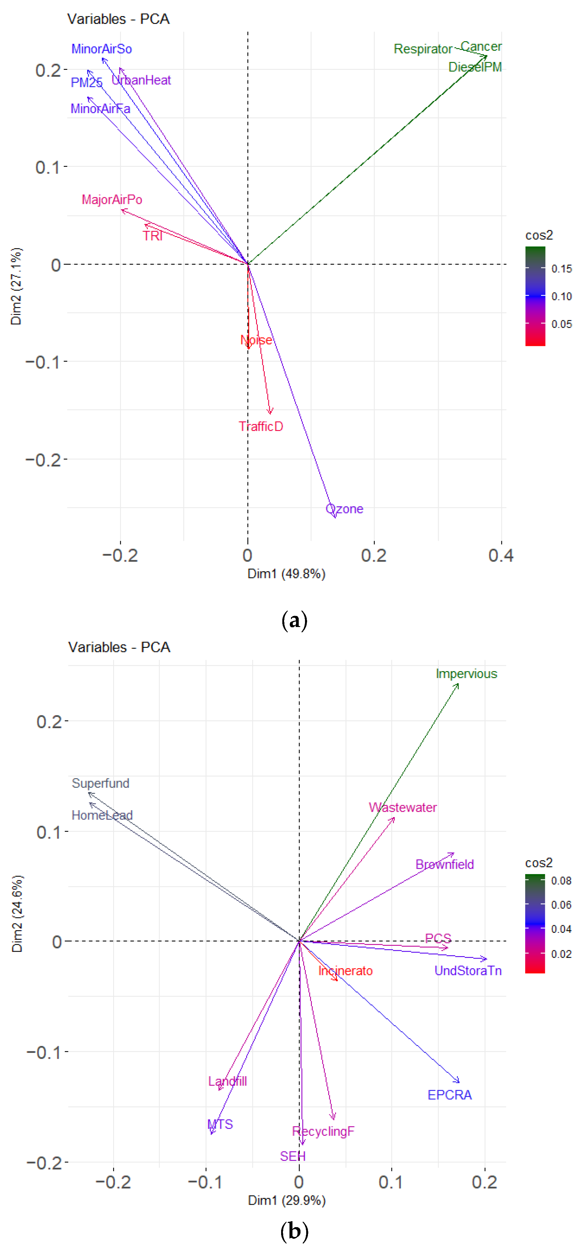
3.2.1. PCA of Potential Pollution Exposure

PC1 and PC2 together explained 76.9% of the variance in Potential_Pollution_Exposure indicators, with PC1 (49.8%) representing urban–industrial air pollution (EPA_AirToxinAssessment_Respiratory_Risk, Diesel_PM_Emissions, EPA_AirToxinAssessment_Cancer_Risk, and PM2.5_Emissions) and PC2 (27.1%) capturing broader air quality (Minor_Air_Sources, Ozone, and Urban_Heat_Island). High cos² values suggest future iterations could streamline this index using only these dominant indicators.

3.2.2. PCA of Potential Pollution Sources

The first two components explained 54.5% of the variance. PC1 (29.9%) highlighted dense urban pollution sources (Impervious_Surfaces, Superfund_Sites, and Housing_Lead_Risk), while PC2 (24.6%) focused on localized waste (Landfills, Wastewater_Discharge, and Recycling_Facilities). High cos² values for impervious surfaces and hazardous facilities support their central role in future pollution source assessments.

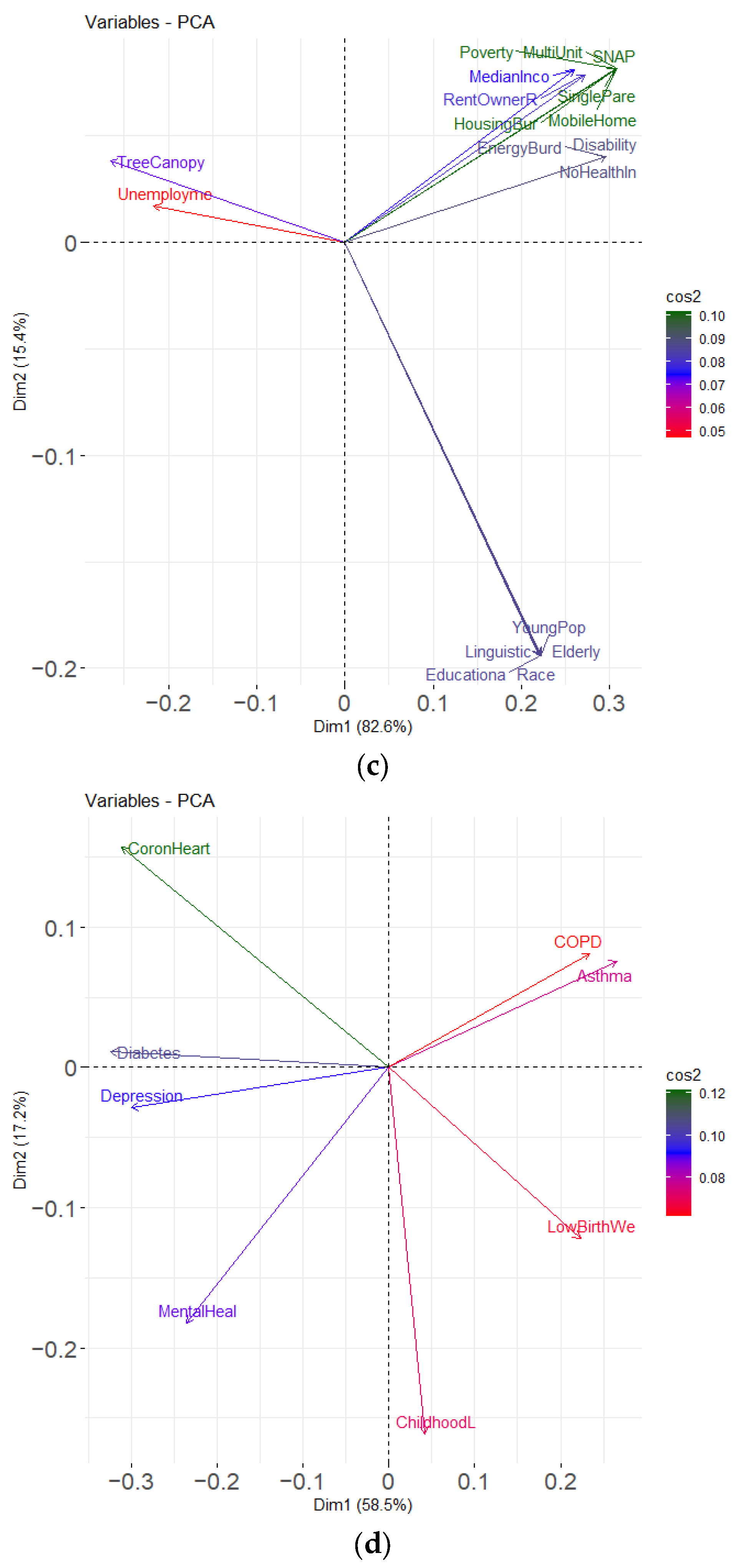
3.2.3. PCA of Health Sensitivity

PC1 and PC2 captured 75.7% of the variance. PC1 (58.5%) reflected chronic disease burden (Coronary_Heart_Disease, Diabetes, Depression, and Poor_Mental_Health), while PC2 (17.2%) reflected respiratory and developmental stressors (Asthma_ER_Visits, COPD, and Childhood_Lead_Exposure).

3.2.4. PCA of Socioeconomic Factors

PC1 (82.6%) and PC2 (15.4%) explained 98% of the variance together. PC1 represented economic strain and housing vulnerability (Food_Insecurity, Mobile_Homes, and Housing_Burden), while PC2 reflected demographic barriers (Linguistic_Isolation, Race, and Median_Income). These results support the separate tracking of economic and demographic stressors in future tools.

3.2.5. PCA of Pollution Burden

PC1 (42.5%) and PC2 (23.6%) explained 66.1% of the variance. PC1 showed large-scale industrial air pollution (Diesel_PM_Emissions, PM2.5_Emissions, EPA_AirToxinsAssessment_Cancer_Risk, and Impervious_Surfaces), while PC2 highlighted land-based waste and hazardous sites (Wastewater_Discharge, Landfills, and Facilities_Releasing_Toxins). These findings support dual-pronged strategies for air and land pollution in high-burden areas.

3.2.6. PCA of Sensitive Populations

PC1 explained 83.1% of the variance in Sensitive_Populations, capturing socioeconomic vulnerability (Single_Parent_Households, Housing_Burden, and Food Insecurity). PC2 (5.8%) explained chronic health burdens (Diabetes, Asthma_ER_Visits, and Depression). These insights validate the strong influence of economic precarity and chronic disease on vulnerability scores.

3.2.7. PCA of Environmental Justice Index

PC1 (71.8%) and PC2 (10.1%) explained 81.9% of the total variance in the EJ_Index. PC1 captured cumulative socioeconomic stressors (Food Insecurity, Housing_Burden, and Poverty), while PC2 represented pollution burdens (Diesel_PM_Emissions, PM2.5_Emissions, and EPA_AirToxinsAssessment_Cancer_Risk). Pollution exposure and socioeconomic indicators emerged as the most critical dimensions of environmental justice disparities.

3.2.8. Key Findings of PCA

Air pollution indicators (Diesel_PM_Emissions, PM2.5_Emissions, and EPA_AirToxinsAssessment_Respiratory_Risk) are the main drivers of the pattern of cumulative environmental disparities. Similarly, socioeconomic factors and health sensitivity indices are strongly influenced by economic stressors (Housing_Burden, Food_Insecurity, and Poverty) and chronic diseases (Coronary_Heart_Disease, Diabetes, and Asthma_ER_Visits). These results suggest that economic disparity (PC1-driven) and pollution burden (PC2-driven) could improve EJScreen’s effectiveness. Also, PCA-driven EJ scores can be used to help state agencies prioritize funding for environmental remediation projects and strengthen compliance monitoring in high-burden census tracts. The dominant PC1 and PC2 contributors should be optimized in future EJScreen tools to make them more policy-applicable. PCA results suggest that CT EJScreen version 2.0 could be optimized by reducing indicator redundancy and refining weighting strategies. The strongest contributors in each category should be prioritized in future iterations to streamline the process without losing key environmental justice insights.

4. Discussion

4.1. Importance in Planning and Policymaking

CT EJScreen provides a data-driven approach for identifying sensitive communities at the census tract scale to help guide equitable resource allocation and support environmental justice decision-making. The tool aids in identifying high-burden areas, prioritizing funding, guiding interagency collaboration, supporting grant applications, and facilitating public education. These applications align with precedents set by other state-specific EJ mapping tools, such as Washington’s identification of “highly impacted communities” [6], California’s Transformative Climate Communities grant program [29], New Jersey’s environmental impact assessments [30], and Colorado’s prioritization of public water system inspections [8,31]. While the ultimate uses of the tool in Connecticut will be decided primarily by state legislators and state agencies, Connecticut shares many characteristics of the other states that have incorporated mapping tools into their policymaking, such as state-administered grant programs, participation in a cap-and-invest program (the Regional Greenhouse Gas Initiative (Regional Greenhouse Gas Initiative https://www.rggi.org/)), and a state-administered permitting process for affecting facilities.

Community feedback sessions emphasized the tool’s practical utility; every audience asked, in essence, the same question: “How do we make our community better with this information?” In response, we prepared a list of starting-point actions inspired by similar mapping tools in other states and by ideas proposed by community participants during the feedback sessions [32]. Any community member can use the tool to understand potential burdens around them and advocate for policy change by engaging with local decision-makers. Community-based organizations can leverage reports from EJScreen to support their advocacy efforts and grant applications, ultimately reaching their equity goals. Municipalities and regional planners can integrate the tool into conservation, hazard mitigation, and economic development plans by targeting highly impacted census tracts to receive necessary investments. At the state level, agencies can use CT EJScreen to prioritize infrastructure funding, assess past practices, refine permitting processes, and enhance environmental justice considerations in grant allocations and policy implementation.

As former state tools influenced CT EJScreen, it may serve as a model for future state-led efforts. Its iterative development process, including extensive beta testing, public engagement, and transparency measures, enhanced usability and trust. The structured process—community-based evaluation forums, advisory committee compensation, public comment periods, and clear documentation of feedback implementation—represents an adaptable model for other states developing their own screening tools.

4.2. Challenges and Limitations of Creating a State-Specific EJScreen

4.2.1. Interpreting and Applying the Tool Correctly

As with any complex tool, CT EJScreen requires initial training to make accurate interpretations and applications of its results. To mitigate this challenge, the tool is available as open-source software, accompanied by supporting materials. However, it is not appropriate for standalone risk assessment purposes and can be misinterpreted without basic training. While correlations might be noted, the tool does not establish causal relationships between environmental toxins and health effects. Policymakers, activists, and researchers using this tool to inform their decision-making must understand this distinction, and good communication should be used to underscore this.

4.2.2. Limitations of Mapping and Data Coverage

CT EJScreen, like all tools created for the task of mapping environmental justice, has inherent limitations linked to both spatial and data extent. Although the tool provides a general analysis of inequalities at the census tract level, the environmental impacts often vary at the neighborhood or single housing unit level. This can lead to underrepresenting highly localized pollution hotspots or socioeconomic vulnerabilities within larger tracts. Large census tracts can mask pollution or vulnerability hotspots, while the lack of statewide datasets related to indoor air quality, drinking water pollution, and residential mold limits the tool’s overall completeness.

Tool variability can stem from a variety of sources, including differences in data sources, spatial resolution differences, and the basic methodological assumptions underlying the analyses. Sources of pollution are usually modeled as discrete point sources, whereas health, socioeconomic, and modeled pollution data can represent larger geographic areas, which may mask localized environmental injustice.

Balancing scientific integrity with community demands for additional indicators remains a key challenge. The current tool aimed to address the concerns of the public to capture cumulative burdens; however, it also introduced potential redundancy, as revealed in the Spearman correlation and PCA analyses. Even though the methodology followed established best practices [4], indicator weighting relies on expert judgment and requires continuous refinement and validation.

4.2.3. Data Accuracy, Timeliness, and Granularity

CT EJScreen relies on the quality, accuracy, completeness, and timeliness of datasets that were available from different sources. Some key limitations include the following:

• Temporal Resolution: There is no standardized frequency of updates on every dataset, leading to potential discrepancies between current conditions and mapped data.
• Geographic Resolution Limitations: The tool operates at the census tract level, which may not accurately reflect smaller-scale discrepancies. Large tracts containing both high- and low-burden areas might receive a low-impact score, despite containing pockets of severe environmental burdens. The opposite case is also possible.
• Data Availability: Certain indicators, such as indoor air pollution, pesticide use, and water contamination, lack comprehensive statewide datasets and are thus excluded from the tool.

4.2.4. Balancing State and Community Priorities

One of the major challenges faced during the development of CT EJScreen was balancing the varying expectations of state agencies and local community groups. State agencies sought a standardized, legally viable tool that was in compliance with existing regulations, while community groups highlighted the need to incorporate experiential information and qualitative data. Although it was not possible to meet every expectation of every party, in general, we tried to prioritize state agency input regarding categorization and presentation of the data layers provided by those agencies or related to their fields of service, while we prioritized community input regarding user-friendliness, accompanying resources, the repository of indicator layers available, and overall clarity. There needs to be an ongoing interaction between policymakers and community groups to balance the scientific credibility of the tool with its ability to reflect public interests.

Some residents expressed concerns about potential misuse of the map (e.g., redlining by financial institutions), while state agencies emphasized their role in directing financial and policy allocations to communities that are both overburdened and under-resourced. Additionally, some stakeholders advocated for the inclusion of community-reported data, but the lack of standardization and verification challenges led us to decide against that. We documented every piece of feedback received during the advisory meetings, community evaluation sessions, and public comment period, and for each piece of feedback, we documented our response, including why we could not or did not implement some of the suggestions. Creating transparency in the use of this tool in decision-making will be critical to building public trust.

4.2.5. Evolving State Goals and the Tool’s Future Development

As the CT EJScreen project progressed, the state changed its priorities and goals for the tool. Originally, the tool was intended to be a comprehensive environmental justice screening tool and a hub to consolidate all relevant information in one place. Since then, the state has decided to separate the cumulative impact assessment from the broader EJ screening process in the upcoming version 3.0. Although this choice allows for more newly oriented in-depth analysis aligned with a recently passed cumulative impact legislation (No. 23-202 [33]), it also raises issues of consistency, ease of use, and compatibility with previous versions. Nevertheless, the lessons learned from Connecticut’s process could be a useful model for other areas in designing their own environmental justice mapping tools.

4.3. Lessons Learned

4.3.1. Balancing Science and Public Needs

One of the key lessons from CT EJScreen’s development is the need to balance statistical independence in data layers with public demand for more indicators. While scientific integrity is key to credibility, adding more layers based on community concerns makes for a more holistic environmental justice assessment. The challenge is to avoid duplication while being relevant, which requires an iterative refinement process guided by both statistical validation and stakeholder input [27].

4.3.2. Refining Data Selection and Indicator Weighting

Future versions should explore more advanced statistical techniques (i.e., PCA weighting on indicators) to refine the weighting mechanism, so index scores accurately reflect environmental justice burdens. Composite index calculations require a robust and transparent weighting approach. Lessons from other composite indices in environmental science (i.e., [25]) suggest being adaptable to new methods is key to long-term tool effectiveness. Additionally, the methodology uses datasets with different update frequencies, which creates inconsistencies. Establishing standardized update protocols and integrating error estimates from sources like the American Community Survey (ACS) will improve long-term reliability.

4.3.3. Ensuring Scientific Integrity Through Nonpartisan Research Facilities

The credibility of environmental justice screening tools depends on the ability to remain objective and independent from political influences, which was accomplished with CT EJScreen version 2.0. To maintain their integrity and avoid political instability, nonpartisan monitoring during the development and upgrade stages is crucial. If these instruments are caught up in unstable political influences, their objectivity and reliability will be put in jeopardy. Creating a research-oriented, nonpartisan body that is tasked with continually upgrading these instruments would create additional buffers against interference from government politics, thus leading to a more open and evidence-driven approach to policy development concerning environmental justice.

4.4. Future Research and Policy Recommendations

4.4.1. Roadmap for CT EJScreen 3.0 and Beyond

Future versions of CT EJScreen should enhance spatial resolution by incorporating finer geographic scales such as block groups where statistically reliable. Also, future tools should seek to leverage emerging technologies, such as machine learning and real-time environmental sensors, to improve accuracy. Additionally, the expansion of datasets to include emerging contaminants and new health trends will increase the tool’s relevance to current environmental and public health challenges [34]. These technologies can enable predictive analytics, more dynamic exposure modeling, and automated data updates. Incorporating emerging contaminants (e.g., PFAS, microplastics) and evolving health trends (e.g., long-term COVID impacts, heat vulnerability) will ensure the tool’s alignment with new environmental and public health research priorities. Future studies can focus on the validity of cumulative burden indices on health outcomes, explore causal pathways linking environmental burdens to health disparities, or test the effectiveness of environmental interventions in high-scoring tracts. Moreover, researchers can refine weighting strategies through comparative analyses of PCA-driven models, Bayesian networks, or ensemble methods.

A critical component of future development is sustained stakeholder engagement. The tool should not merely serve as a technical platform but as a communal framework that embraces input from policymakers, researchers, and community stakeholders. Establishing feedback mechanisms and routine iterative revisions will support continual improvement and long-term use over time.

4.4.2. Integrating CT EJScreen into Decision-Making

• Regulatory Integration: Use CT EJScreen in permitting and land use planning to address cumulative environmental impacts and enforce stricter reviews in high-impact areas. High-impact areas can be defined as those with EJ_Index scores between 6 and 10. At the same time, a broader review of all ranks should be encouraged to capture emerging or context-specific vulnerabilities.
• Resource Allocation: Prioritize funding for green infrastructure, renewable energy, resilience programs, and environmental remediation in overburdened communities.
• Community Engagement: Expand the integration of the tool and environmental justice into the education curriculum and improve data transparency to support public awareness and local advocacy efforts.
• Cross-Agency Collaboration: Establish an interagency task force to standardize tool use across sectors and collaborate with academic institutions to refine methodologies and datasets.

5. Conclusions

This study describes the Connecticut Environmental Justice Screening Tool (CT EJScreen), detailing its development, methodology, statistical analyses, and policy applications. Spearman correlation and Principal Component Analysis (PCA) identified key indicators driving cumulative indices, highlighting opportunities to refine variable selection, weighting methodologies, and policy applications. CT EJScreen is a significant step in state-level environmental justice mapping, as it overcomes the limitations of federal tools by incorporating localized data and community input. Its use of state-specific data coupled with statistical modeling makes it a standard for adaptive and transparent environmental justice policy.

CT EJScreen should evolve to meet the changing policy and research needs. Future improvements should prioritize PCA-driven weighting refinements and expand regulatory integration. By integrating CT EJScreen into Connecticut’s environmental justice policy framework, the state can ensure ongoing utility as a regulatory measure tool, funding allocation, and environmental health protection. The lessons learned can be a model for other states developing EJ screening tools, advancing equitable and data-driven environmental policies nationally.

References

1. United States Environmental Protection Agency. How Was EJScreen Developed? Available online: https://19january2021snapshot.epa.gov/ejscreen/how-was-ejscreen-developed_.html#:~:text=Development%20of%20EJSCREEN%20began%20in,newest%20and%20best%20data%20available. (accessed on 10 May 2025).
2. Centers for Disease Control and Prevention, Agency for Toxic Substances and Disease Registry. Environmental Justice Index. Available online: https://www.atsdr.cdc.gov/place-health/php/eji/?CDC_AAref_Val=https://www.atsdr.cdc.gov/placeandhealth/eji/index.html (accessed on 12 May 2025).
3. Council on Environmental Quality Climate and Economic Justice Screening Tool. Available online: https://ndcpartnership.org/knowledge-portal/climate-toolbox/climate-and-economic-justice-screening-tool-cejst#:~:text=The%20tool%20has%20an%20interactive,that%20are%20experiencing%20these%20burdens (accessed on 10 May 2025).
4. Meehan August, L.; Faust, J.B.; Cushing, L.; Zeise, L.; Alexeeff, G.V. Methodological Considerations in Screening for Cumulative Environmental Health Impacts: Lessons Learned from a Pilot Study in California. Int. J. Environ. Res. Public Health 2012, 9, 3069–3084. [Google Scholar] [CrossRef] [PubMed]
5. United States Environmental Protection Agency. How Does EPA Use EJScreen? Available online: https://19january2017snapshot.epa.gov/ejscreen/how-does-epa-use-ejscreen_.html (accessed on 10 May 2025).
6. Min, E.; Gruen, D.; Banerjee, D.; Echeverria, T.; Freelander, L.; Schmeltz, M.; Saganić, E.; Piazza, M.; Galaviz, V.E.; Yost, M.; et al. The Washington State Environmental Health Disparities Map: Development of a Community-Responsive Cumulative Impacts Assessment Tool. Int. J. Environ. Res. Public Health 2019, 16, 4470. [Google Scholar] [CrossRef] [PubMed]
7. Konisky, D.; Gonzalez, D.; Leatherman, K. Mapping for Environmental Justice: An Analysis of State Level Tools; Environmental Resilience Institute at Indiana University: Bloomington, IN, USA, 2021. [Google Scholar]
8. Colorado EnviroScreen 2.0 Team. Colorado EnviroScreen Tool Technical Document; Colorado EnviroScreen 2.0 Team: Denver, CO, USA, 2024. [Google Scholar]
9. August, L.; Bangia, K.; Plummer, L.; Prasad, S.; Ranjbar, K.; Slocombe, A.; Wieland, W. Office of Environmental Health Hazard Assessment, CalEnviroScreen 4.0. 2021. Available online: https://oehha.ca.gov/media/downloads/calenviroscreen/report/calenviroscreen40reportf2021.pdf (accessed on 10 May 2025).
10. Kruse, K.; Bunting, A.; Esch, J.; Goodwin, K.; Vandenberg, C.; Albright, D.; Allen, D.; Office of the Environmental Justice Public Advocate. MiEJScreen Michigan Environmental Justice Mapping and Screening Tool. 2022. Available online: https://www.michigan.gov/egle/-/media/Project/Websites/egle/Documents/Maps-Data/MiEJScreen/Report-2024-07-MiEJScreen-Technical.pdf (accessed on 10 May 2025).
11. Department of Environmental; Occupational Health Sciences, University of Washington; Washington State Department of Health. Washington Environmental Health Disparities Map: Cumulative Impacts of Environmental Health Risk Factors Across Communities of Washington State; Washington State Department of Health: Washington, DC, USA, 2019. [Google Scholar]
12. Sotolongo, M. Defining Environmental Justice Communities: Evaluating Digital Infrastructure in Southeastern States for Justice40 Benefits Allocation. Appl. Geogr. 2023, 158, 103057. [Google Scholar] [CrossRef]
13. Onat, Y.; Buchanan, M.; Wozniak-Brown, J.; Massidda, C.; Duskin, L.; Alpdogan, D.; Morris, K.; Torres, A.; Peate, B.; Pimenta, M.; et al. CT Environmental Justice Screening Tool Report—Version 2.0; University of Connecticut: Groton, CT, USA, 2023. [Google Scholar] [CrossRef]
14. United States Environmental Protection Agency. What Is EJSCREEN? | EJSCREEN: Environmental Justice Screening and Mapping Tool; US EPA: Washington, DC, USA, 2019; pp. 1–17. [Google Scholar]
15. Besse, H.; Rojas-Rueda, D. Environmental Justice Mapping Tools in the United States: A Review of National and State Tools. Sci. Total Environ. 2025, 962, 178449. [Google Scholar] [CrossRef] [PubMed]
16. del Fierro, S.; McInerney, E.; Musco, J.; Swab, E.; Teirstein, M.; Engelman-Lado, M. Scoping and Recommendations for the Development of a Connecticut Environmental Justice Mapping Tool; Yale University: New Haven, CT, USA, 2021. [Google Scholar]
17. Heaney, C.D.; Wing, S.; Campbell, R.L.; Caldwell, D.; Hopkins, B.; Richardson, D.; Yeatts, K. Relation between Malodor, Ambient Hydrogen Sulfide, and Health in a Community Bordering a Landfill. Environ. Res. 2011, 111, 847–852. [Google Scholar] [CrossRef] [PubMed]
18. Requia, W.J.; Di, Q.; Silvern, R.; Kelly, J.T.; Koutrakis, P.; Mickley, L.J.; Sulprizio, M.P.; Amini, H.; Shi, L.; Schwartz, J. An Ensemble Learning Approach for Estimating High Spatiotemporal Resolution of Ground-Level Ozone in the Contiguous United States. Environ. Sci. Technol. 2020, 54, 11037–11047. [Google Scholar] [CrossRef] [PubMed]
19. Van Donkelaar, A.; Hammer, M.S.; Bindle, L.; Brauer, M.; Brook, J.R.; Garay, M.J.; Hsu, N.C.; Kalashnikova, O.V.; Kahn, R.A.; Lee, C.; et al. Monthly Global Estimates of Fine Particulate Matter and Their Uncertainty. Environ. Sci. Technol. 2021, 55, 15287–15300. [Google Scholar] [CrossRef] [PubMed]
20. Alexeeff, G.V.; Faust, J.B.; August, L.M.; Milanes, C.; Randles, K.; Zeise, L.; Denton, J. A Screening Method for Assessing Cumulative Impacts. Int. J. Environ. Res. Public Health 2012, 9, 648–659. [Google Scholar] [CrossRef] [PubMed]
21. Morello-Frosch, R.; Pastor, M.; Porras, C.; Sadd, J. Environmental Justice and Regional Inequality in Southern California: Implications for Future Research. Environ. Health Perspect. 2002, 110, 149–154. [Google Scholar] [CrossRef] [PubMed]
22. Huang, H.; Wang, A.; Morello-Frosch, R.; Lam, J.; Sirota, M.; Padula, A.; Woodruff, T.J. Cumulative Risk and Impact Modeling on Environmental Chemical and Social Stressors. Curr. Environ. Health Rep. 2018, 5, 88–99. [Google Scholar] [CrossRef] [PubMed]
23. Krieg, E.J.; Faber, D.R. Not so Black and White: Environmental Justice and Cumulative Impact Assessments. Environ. Impact Assess. Rev. 2004, 24, 667–694. [Google Scholar] [CrossRef]
24. Murphy, S.R.; Prasad, S.B.; Faust, J.B.; Alexeeff, G.V. Community-Based Cumulative Impact Assessment: California’s Approach to Integrating Nonchemical Stressors into Environmental Assessment Practices. In Chemical Mixtures and Combined Chemical and Nonchemical Stressors; Springer: Cham, Switzerland, 2018; pp. 515–544. ISBN 9783319562322. [Google Scholar]
25. Lee, C. A Game Changer in the Making? Lessons From Advancing Strategies, Environmental Justice through Mapping and Cumulative Impact Strategies. Environ. Law Inst. 2009, 50, 10203–10215. [Google Scholar]
26. Brody, T.M.; Di Bianca, P.; Krysa, J. Analysis of Inland Crude Oil Spill Threats, Vulnerabilities, and Emergency Response in the Midwest United States. Risk Anal. 2012, 32, 1741–1749. [Google Scholar] [CrossRef] [PubMed]
27. Morello-Frosch, R.; Jesdale, B.M. Separate and Unequal: Residential Segregation and Estimated Cancer Risks Associated with Ambient Air Toxins in U.S. Metropolitan Areas. Environ. Health Perspect. 2006, 114, 386–393. [Google Scholar] [CrossRef] [PubMed]
28. Connecticut General Assembly. Connecticut General Statutes § 22a-20a—Environmental Justice; Connecticut General Assembly: Hartford, CT, USA, 2023; Sec.22a-20a. [Google Scholar]
29. California Strategic Growth Council Transformative Climate Communities: Community-Led Transformation for a Sustainable California. Available online: https://sgc.ca.gov/programs/TCC/ (accessed on 6 November 2023).
30. New Jersey Department of Environmental Protection Environmental Justice Law. Available online: https://dep.nj.gov/ej/law/ (accessed on 6 November 2023).
31. Colorado Environmental Public Health Tracking Colorado EnviroScreen: An Environmental Justice Mapping Tool. Available online: https://coepht.colorado.gov/blog-post/colorado-enviroscreen-an-environmental-justice-mapping-tool (accessed on 6 November 2023).
32. Connecticut Institute for Resilience and Climate Adaptation (CIRCA) Ideas for What to Do With the CT EJ Screening Tool. Available online: https://connecticut-environmental-justice.circa.uconn.edu/now-what-actions-after-ct-ej-screening-tool/ (accessed on 6 November 2023).
33. Connecticut General Assembly. An Act Concerning the Environmental Justice Program of the Department of Energy and Environmental Protection; Connecticut General Assembly: Hartford, CT, USA, 2023; Substitute Senate Bill No. 1147. [Google Scholar]
34. Kloog, I.; Chudnovsky, A.A.; Just, A.C.; Nordio, F.; Koutrakis, P.; Coull, B.A.; Lyapustin, A.; Wang, Y.; Schwartz, J. A New Hybrid Spatio-Temporal Model for Estimating Daily Multi-Year PM2.5 Concentrations across Northeastern USA Using High Resolution Aerosol Optical Depth Data. Atmos. Environ. 2014, 95, 581–590. [Google Scholar] [CrossRef] [PubMed]
Figure 1. CT EJScreen version 2.0 web interface. The first layer shown on the map is the EJ_Index, with tracts highlighted in darker to lighter shading. The darker the colors on the tract, the higher the potential cumulative index values represented. All the sub-category indicator layers can be toggled on and off and are grouped under their categories with respective icons (Marked A). Additionally, the tool has features for easy navigation, such as typing an address, zooming in/out, returning to the home view, and location sharing (Marked B), as shown in the figure. In the top right corner (Marked C), the tool has the following widgets arranged from left to right: Legend, Context Layers, Boundaries, Basemap Gallery, Info Page, How to use the App, Swipe, Chart, Print, Report, Filter, Bookmark, Select and Add Data.
Sustainability 17 04535 g001
Figure 2. Spearman analysis coefficients of the indicators of CT EJScreen version 2.0.
Sustainability 17 04535 g002
Figure 3. Principal Component Analysis (PCA) plots for key indices in CT EJScreen. The visualization of PCA results in biplots (Figure 3) helps users see clustering of similar indicators and their directional contribution to each component. The axes represent the proportion of variance explained by PC1 and PC2, which together capture most of the variability in each dataset. Vectors represent individual indicators, and their orientation and length indicate their influence on each component. Indicators pointing in the same direction are positively correlated, while those at opposing angles are negatively correlated. The cos2 values indicate the contribution of each variable to the principal components—higher values (green) indicate stronger contributions to the selected components, while lower values (red/blue) imply a weaker influence. (a) Pollution Exposure: PC1 (49.8%) explains urban–industrial air pollution, while PC2 (27.1%) captures broader air quality impacts; (b) Pollution Sources: PC1 (29.9%) represents impervious surfaces and industrial pollution, while PC2 (24.6%) highlights waste-related contamination; (c) Socioeconomic Factors: PC1 (82.6%) captures economic and housing stressors, while PC2 (15.4%) represents demographic disparities; (d) Health Sensitivity: PC1 (58.5%) captures chronic disease patterns, while PC2 (17.2%) represents respiratory and developmental health burdens.
Sustainability 17 04535 g003aSustainability 17 04535 g003b