Article

Performance Evaluation of Computational Fluid Dynamics and Gaussian Plume Models: Their Application in the Prairie Grass Project

by
Ruben Cabello
1,
Carles Troyano Ferré
1,
Alexandra Elena Plesu Popescu
1,
Jordi Bonet
1,
Joan Llorens
1 and
Raúl Arasa Agudo
2,*
1
Department of Chemical Engineering and Analytical Chemistry, University of Barcelona, Martí I Franquès, 1, 08028 Barcelona, Spain
2
Applied Research, Meteosim, Baldiri I Reixac 10th, 08028 Barcelona, Spain
*
Author to whom correspondence should be addressed.
Sustainability 2025, 17(10), 4403; https://doi.org/10.3390/su17104403
Submission received: 6 February 2025 / Revised: 19 April 2025 / Accepted: 7 May 2025 / Published: 12 May 2025
(This article belongs to the Section Energy Sustainability)

Abstract

:
Nowadays, industries and society are very concerned about pollution, well-being, health, air quality, and the possible negative effects of industrial emissions on a property’s surroundings. This gas dispersion is typically estimated with Gaussian Plume/Puff Models or software that uses these models with slight adjustments. The issue regarding these models is that they do not consider the surroundings’ particularities, for instance, when obstacles are present, and they require experimental data to adapt to specific scenarios. Therefore, the aim of this work is to validate the use of ANSYS Fluent® 2022 R1 for modelling atmospheric gas dispersion. This validation is performed by comparing the ANSYS Fluent® 2022 R1 findings to published experimental data, Gaussian Plume Models (GPM in this case corresponds to the application of the Gaussian Equation or Gaussian Fit, and does not correspond to a specific dispersion model), and ALOHA 5.4.7 software. A comparison between these three alternatives was not available in the literature. In terms of downwind dispersion, the findings of the three models are extremely comparable. However, ANSYS Fluent® has a propensity to overestimate the concentration at higher heights. Validation using ANSYS Fluent® in atmospheric gas dispersion applications enables confident results to be obtained in other scenarios. Differences in pollutant estimation between models are clear when studying more complex cases containing turbulence-inducing geometries. In these cases, CFD exhibits a more realistic description of the transport phenomena than the other models considered. The Prairie Grass Project is used as a tool to validate the CFD model, and to demonstrate its potential for more complex cases.

1. Introduction

Atmospheric pollution is acknowledged as one of the main societal issues [1,2], having a high impact on human health [3] and ecosystems and contributing to climate change [4]. Consequently, both wealthy and developing countries often experience episodes of poor air quality. This poor air quality is not only due to anthropogenic emissions, mainly from traffic and industry, but also from natural emissions, such as dust [5] from arid or semiarid regions, which may be carried over considerable distances. In this context, air quality modelling represents a relevant tool for managing air quality and atmospheric pollution, benefiting both public administration and the private sector, and promoting more sustainable cities and regions.
Gas dispersion is a highly studied topic due to its great relevance, whether in unit operations, safety and risk assessment issues, or in determining the possible environmental or human health impacts. Atmospheric gas dispersion is particularly important for assessing pollutant concentrations at a specific location point under given conditions related to air quality and for estimating any potential effects on human health. Pollution and air quality are two very pressing concerns in society. As a consequence of this, recently, the European Union has approved a new Ambient Air Quality Directive which sets more restrictive limit values, focuses on modelling as a tool to improve air quality management, and prepares the legal framework to establish more effective and exhaustive action and short-term plans [6]. This will have indirect effects over industrial emissions. Modelling tools, as used in this paper, will have a more relevant role in this legal framework during the following years in comparison with previous Directives.
The investigation of the atmospheric dispersion of pollutants arose some time ago with the use of flues to dilute stuffs. Nowadays, it is also important to be able to foresee the effects of accidental emissions of polluting or toxic substances on the impact area [7] or to locate the origin of a leak [8]. However, this is a subject that is still being studied because of its immense complexity and the fact that there are many variables to consider [9], for example, the wind velocity, temperature, or solar radiation, among others. Due to its relevance, many experiments have been carried out since the 1950s. As a result, a significant amount of data are available for diverse climatic conditions, terrains, and substances. Chang and Hanna summed up a collection of atmospheric dispersion data sets [10].
To briefly mention a few atmospheric dispersion data sets, Dipole Pride 26’s experiments studied instantaneous and continuous SF6 discharges at the ground level. The concentration measurements were taken in arcs about one, five, and twenty kilometres downwind of the source. In this case, radiosondes and pilot balloon stations were used to gather meteorological data [11]. Another example of the experimental data summed up in Chang and Hanna is the FLADIS case, in which the investigation focused on continuous NH3 dispersion [10]. The gas emissions were about 0.5 kg NH3/s for 20 min. Concentration measurements were taken using sensors located in arcs at 20 m, 70 m, and 240 m intervals [11]. Despite there being data of several dispersion cases, the Prairie Grass Project stands out for its available data, which is obtainable on the Irwin website [12].
The Prairie Grass Project, conducted in 1956 near O’Neill, Nebraska, was an atmospheric dispersion study designed to quantify the diffusion of tracer gases, specifically sulphur dioxide, over grassland terrain under diverse meteorological conditions. Measures of tracer concentrations at various downwind distances and different heights were performed (up to 70 tracer data collection periods) and correlated with detailed meteorological data. The Prairie Grass Project used a methodical approach to the sampling and release of the tracer. With the exception of trials 63–68, when the height was changed to 1.5 m, SO2 was continuously discharged horizontally from a two-inch plastic pipe at a height of 0.46 m. Receptors were placed at a height of 1.5 m, and downwind sampling was carried out across five semicircular arcs at 50, 100, 200, 400, and 800 m. Each arc was 180 degrees long and centred on the release; the outermost 800 m arc had a receptor spacing of one degree, while the inner four arcs had a spacing of two degrees. The semicircle was covered from west to east. Six lightweight metal towers were positioned at 14-degree intervals around the 100 m arc to measure vertical dispersion, yielding samples at nine different heights ranging from 0.5 to 17.5 m. During the field experiments, meteorological data were collected at two distinct locations, both at a height of 2 m above the ground. These locations were as follows: (a) 25 m west of the tracer release point, and (b) 450 m downwind and 30 m west of the centre of the receptor array. Meteorological results were analyzed for both the 10 min and 20 min periods. Notably, the 20 min period encompassed the 10 min tracer sampling period, starting 5 min prior. At the release location, the 10 min meteorological data directly coincided with the 10 min tracer sampling. However, at the downwind location, the start of the 10 min meteorological data was delayed by the travel time of the plume. The aim of the Prairie Grass Project was to provide empirical data for enhancing atmospheric dispersion models. Their experiments established a foundation for understanding how gases move through the lower atmosphere, making it a landmark study in atmospheric science. Semi-empirical models were developed from the collected data, such as those data from the Prairie Grass Project [10] whose field data are usually used in the literature as a reference [13].
These semi-empirical models are commonly used to authorize industrial sources and assess the risk of hazardous leaks in legal situations [14], and therefore, this study focuses on its collected data. Moreover, public safety and security can be enhanced by modelling and understanding the repercussions of a failure, such as a natural gas pipeline breakdown [15] or a nuclear plant failure [16]. Given the necessity for highly dependable estimations, these models have been refined throughout the years. In addition, some software appeared to make calculations easier to manage. Areal Location of Hazardous Atmosphere (ALOHA) [17] is especially famous for modelling accidents like atmospheric gas releases [18] and therefore will be considered as a basis for comparison in this study. Although the semi-empirical models have been extended to some simple geometries, such as in the case of parallel boundaries [19], the semi-empirical models do not consider the details and particularities of the scenario.
Semi-empirical models such as ALOHA usually work in defined meteorological conditions, such as considering atmospheric stability, and do not consider the real atmospheric conditions. The following paragraph presents some cases where the semi-empirical models have been applied and the next one presents some cases where Computational Fluid Dynamics (CFD) is required. Although CFD results are not used nowadays as a legal reference, in the case of complex scenarios, they provide valuable information to various stakeholders such as authorities, decision-makers, or even air quality modellers [20]. Studies supporting the validity of CFD results and providing reference parameters for the simulation are required to provide legal validity to CFD versus the classically used tools.
Pakchotanon et al. study the consequences of an accidental amine leak in the carbon capture and storage system of a coal-fired power plant located in Saskatchewan, Canada [21]. In particular, the CALPUFF model (a Lagrangian Gaussian Puff dispersion model) is used to find the concentration at ground level. Because air speed and velocity vary throughout the year, various simulated concentration distributions are seen depending on the season [21]. This shows that air velocity has a significant impact on gas dispersion. The dispersion of pollutants is conditioned at a meteorological level fundamentally by three factors: large-scale meteorological factors, such as the presence of persistent anticyclones [22]; atmospheric stratification for vertical dispersion [22,23], such as when thermal inversions occur; and topographic and local effects, such as when pollutants are transported by sea breezes or drainage winds [24,25,26]. Iskender is concerned about the industrial utilization risks of acetone [27], a very common chemical. Therefore, a storage tank release is carried out with ALOHA obtaining the risk distribution zones [27]. Ahmad et al. investigate the best location to build a methanol plant’s reactor, avoiding any deaths in the surrounding area in case of an accident [28]. HYSYS software is used to characterize the chemical mixture release before calculating the effect with ALOHA [28].
The inverse problem is likewise addressed: the acquired data indicates a release, but its location is unclear. Sánchez-Pérez et al. forecast the position, release time, and mass release rate of an unknown gas emission using ALOHA software and Matlab programming [29]. Shojaee Barjoee et al. reflect on the need to compare the different models to determine which is most appropriate for each case [30]. Mouilleau et al. discuss the validation of discharge and subsequent atmospheric dispersion for both unpressurised and pressurized carbon dioxide releases using the consequence modelling package PHAST [31]. Particularly, ALOHA and PHAST are compared, and the results show that PHAST is more conservative. The empirical results of an LNG road tank discharge under class B atmospheric conditions show a similar gas propagation to that obtained using the Gaussian gas model of EFFECTS software [32].
Despite their widespread use, some of these models contain scenarios in which the estimation of concentration is inaccurate, for example, in complex terrain, in the presence of obstacles, with chemical reactions like combustion [33], with very low wind speeds, or in the presence of dense gases, among others. In these cases, there is a tendency to resort to wind tunnel experiments or CFD simulations [34]. Gant et al. [35] review the challenges of CFD dispersion modelling, which include the reliable representation of atmospheric boundary layers, suitable grid resolution, and model variability. But according to Wang et al., CFD software is able to simulate and visualize plume drift more precisely than a Gaussian diffusion model or wind tunnel tests [36]. In this sense, CFD programmes such as ANSYS Fluent® [37] may be used to assess the abovementioned situations; however, they require a mesh that can adjust to the features of the terrain.
There are many examples showing the applicability of CFD to complex terrains and urban areas. Gianfelice et al. accurately predict the wind conditions in a complex terrain such as Toronto city [38]. They find that CFD can provide real-time estimations of the wind field at multiple elevations. Oliver et al. analyze the emissions produced by a large emitter in the surroundings of Barcelona [39]. This research utilizes a mesoscale meteorological model with a minimal resolution of up to 1 km. They remark on the necessity of comparing their model against other subgrid-scale methods. CFD allows street canyon ventilation enhancement to be studied by using wind flow deflectors [40] or by strategically planting trees [41]. Shen et al. highlight the importance of the presence, number, and location of inlet boundary conditions for gas dispersion cases, as they greatly impact turbulence and wind speed in the domain [42]. These reviewed articles show the importance that the mesh generation and boundary conditions have on the accuracy of the results.
Since there are many different cases and a lot of variables involved, more experimental data are needed to validate CFD studies and ensure they use good approaches]. Schleder et al. review wind flow studies around buildings, because a correct simulation highly depends on an accurate modelling of the wind flow [43]. CFD is more widely used in aerospace engineering than in any other field. Escarti-Guillem et al. predict the unsteady plume resulting from a rocket by using OpenFOAM [44]. Synylo et al. analyze, using the OpenFOAM CFD code, the pollutant plumes produced by aircraft near airports to improve air quality [45].
In recent years, CFD has seen an increase in its usage for safety and environmental problems. San José et al. use CFD modelling to infer the effects of climate change on the temperature and air pollution of urban areas [46]. They then estimate the cost on human health that climate change will have on the next 10 to 80 years. Hanjalic and Kenjeres simulate the pollutant accumulation in a town when the atmosphere is capped by an inversion layer, which is a weather condition that prevents the pollutant from leaving the region [47]. Wójtowicz-Wróbel et al. recreate a typical urban domain in non-central areas and numerically investigate the dispersion of gases produced by a thermal waste treatment plant in various wind directions [48]. Xin et al. study dispersion on uneven mountain terrain over various kilometres [49]. They find how the rough terrain greatly impacts the diffusion mechanisms.
Mehdi and Panin study the gas dispersion in complex terrain, concluding that RANS turbulence models, particularly the k-Ɛ model, are adequate for such situations [50]. Akhter et al. simulate the pollutant dispersion in urban areas with a k-Ɛ model and conclude that the building height has a high impact on dispersing pollutants [51]. Using data from a real fire in an urban area, Clements et al. compare CFD (LES model) with GPM (Gaussian Plume Model) [52]: CFD provides a higher resolution and accuracy and is more flexible to include physical parameters such as wind vertical profiles or the fire buoyancy effect but requires more computational power and skills to properly implement and simulate the case to obtain reliable results. Although nowadays the GPM provides a real time response, increasing computer power can also provide, in the near future, a fast response for CFD. Da Silva et al. confirm the SST turbulence model with results obtained from a wind tunnel [53] and then analyze the breathability in a city [54]. Determining the most likely location of an unknown pollutant release is also possible with CFD. Particularly, Sharma et al. provide a quick, accurate, and efficient approach for determining the location of contamination sources in real time [55]. A CFD model is not limited to open spaces but can also be used also for closed spaces, e.g., a leakage in a utility tunnel [56].
Semi-empirical models, which are based on the classical Gaussian Plume Model, are widely used and have been implemented in specialized software such as ALOHA. Nevertheless, when the terrain has some particularities that differ from the original conditions where the semi-empirical model parameters were regressed, e.g., the presence of any obstacles, then CFD simulation is applied. CFD has been increasingly applied to atmospheric gas dispersion problems, especially for scenarios where semi-empirical models are considered not suitable or reliable. However, CFD also has some challenges and limitations, such as the computational cost and time. This study directly compares, for a specific gas dispersion scenario, the experimental data with CFD simulations, ALOHA, and the application of the Gaussian Equation (referred to as Gaussian Plume Model, GPM). Two different models, or a model and CFD, were previously compared, but this work uniquely integrates all three elements, clearly showing their strengths and weaknesses in predicting real-world gas dispersion. The insights gained from this validated CFD model underline the reliability of the CFD simulation and serve as a basis for creating better forecasting techniques.
This research is focused on potential emissions injected into the atmosphere in emergencies or accidental situations, and how we can analyze the dispersion of these pollutants in the atmosphere and their effects over near receptors.

2. Materials and Methods

The material and methods described here are used to check the reliability of CFD as a tool for predicting an atmospheric dispersion of a gas. Particularly, the CFD analysis is carried out with the SST k-ω model, which is commonly used in the literature reviewed. To evaluate the model’s accuracy, a diverse set of experiments from the Prairie Grass Project, specifically releases n° #5, #9, #11, #15, #16, #18, #19, #22, #26, #31–33, #39, #42, #44, #54, #56, #59, and #61, encompassing a range of meteorological conditions and release scenarios, are simulated and subsequently compared against the corresponding empirical measurements. Concentration is also predicted with a Gaussian Plume Model (GPM) and ALOHA and is critically compared with the CFD results. The GPM corresponds to the application of the Gaussian equation or Gaussian fit. To compare the CFD modelling carried out, we have selected GPM and ALOHA [17] because our analysis is focused on the effects of pollutants injected into the atmosphere over distances less than 500 m–1 km. Other models, like CALPUFF [57], have difficulties obtaining accurate results in receptors near the sources in comparison to other Gaussian models like AERMOD [58].

2.1. Material

The material used in this investigation is a computer with an Intel® Core i9-10940X processor and an NVIDIA Quadro RTX 5000 graphics card. On this computer, the CFD simulation run with ANSYS Fluent® 2022 R1 requires around six computing hours per studied case. The additional modelling tools used are Gaussian Plume Modelling and ALOHA 5.4.7 software.

2.2. Simulation Setup

The domain for the CFD simulation is a rectangular base prism with a release pipe positioned 50 m away from the prism base (Figure 1). It is made up of two inlets (air and emission), an outlet, and four walls (top, bottom, right, and left side). The bottom wall is defined as a no-slip boundary condition. The other walls are set to have zero shear stress, as if the air flowing outside the domain has the same velocity as the air flowing by the wall, or in other words, there is a zero velocity gradient towards the wall.
The domain dimensions to simulate the atmospheric gas dispersion, which are shown in Table 1, are chosen based on the experimental data collected from the Prairie Grass Project [59] and the computational time and cost.
The simulation setup mirrors the Prairie Grass experiment (near O’Neill, Nebraska, summer 1956), replicating the emission source and dimensions up to the measurement locations. Although the experiment included sampling up to 800 m, these furthest measurements are excluded from our analysis due to the significant computational cost and time associated with long-distance CFD simulations. The computational domain’s width and height are determined to prevent the artificial confinement of the plume, since the domain boundaries (top, bottom, right, and left) are treated as walls. An adequate domain width and height must ensure that the plume does not reach these boundary walls with a significant pollutant concentration, which could skew results. A maximum concentration threshold of 0.5 mg/m3 at the domain walls is used as a criterion, which is significantly lower than plume core concentrations, and preliminary simulations confirm that this limit is not exceeded with the chosen domain size.
The furthest studied point from the Prairie Grass Project is the 400 m point. The domain is lengthened by 50 m before the emission source and after the 400 m point, leading to a 500 m total domain, to ensure that inlet and outlet boundary conditions do not affect the simulation results. Considering the aforementioned information, the final dimensions of the domain are summarized in Table 1. The selected dimensions are like those found in Zhang et al. [60], where a risk analysis of toxic gas leakage is performed with CFD for a real gas gathering station of H2S.
All geometries and simulations are created and performed in ANSYS 2022 R1. The turbulence model, the energy equation, and the species transport equation used are implemented in this software. In particular, the selected models are the SST k-ω, as it smoothly blends wall resolving k-ω equations for near-the-ground phenomena, and the k-ε model, for bulk-free shear air flow in upper layers. The SST model provides acceptable results for a gas dispersion study comparing various turbulent models [61]. Further details on this model can be found in ANSYS Fluent Theory Guide [62]. The simulation employs pseudo-transient time-advancement iterations to facilitate convergence to the steady-state solution. The specified gas mixture contains air and the studied species, which, in the case of the Prairie Grass Project, is sulphur dioxide (SO2) [59]. Pure SO2 is fed into the emission inlet at the same ratio as performed in the experiment. It is important to note that SO2 gas is a relatively inert pollutant in the atmosphere, which aids in comparing the different models, as ALOHA and GPM are unable to estimate the reactivity of gases. The differences between these models and experimental results would likely be more pronounced if a more reactive pollutant had been used.
Different meshes are created to determine the configuration that allows the minimum cell number and does not affect the results (mesh independence study). The unstructured polyhedral mesh has been used for its capacity to fill the space without considerably increasing the number of nodes. This type of mesh is commonly used to increase efficiency and accuracy [63] and it has been used for all of the simulations in this study. To properly represent the concentration curve, we refine the cells where the concentration gradient is large. We do this by calculating a mesh correction function and, where this function exceeds the refinement criteria, the cell is divided into six different cells. We do this iteratively with the refinement performed six times in total at intervals of 50 iterations. A mesh correction function that depends on the CRL (the Cell Refine Level: the number of times the cell has already been divided) is implemented (Equation (1)). The factor 2−3·CRL ensures no excessive refinement, avoiding extra computational costs. Only the high gradient cells are refined further. This function is evaluated in all cells, and those whose value is over the refinement criteria are further refined. Cells are also refined if they are in the vicinity of a solid boundary. The selected solution algorithm to resolve the simulations is coupled.
f M e s h C o r r e c t i o n = X p · 2 3 · C R L ,
An ideal gas model is used for estimating the density of the gases involved. The other air properties are kept constant. For the SO2, the specific heat is set as a piecewise polynomial, and the thermal conductivity and viscosity are calculated with the kinetic theory. Mixture properties are evaluated using the mixing law approximation, except for the mass diffusivity, where kinetic theory is applied [62]. The solar radiation intensity generates a temperature gradient between heights. A heat flux at the ground surface is used to simulate this phenomenon, assuming the radiation bounces off the ground in the form of heat and is not absorbed by the chemical compounds of the domain. The side walls are adiabatic. The accumulation of thermal energy is prevented by restricting the top side to the same heat flow as the bottom. An initial simulation is run to estimate the temperature profile at the outlet and to use this as the inlet boundary condition. By addressing the simulation in this manner, a stabilized temperature profile is created in the domain which describes the atmospheric conditions.
The air inlet is defined with three formulas which are presented in Open Foam [64]: the velocity profile regarding the height, the turbulent kinetic energy (k), and the dissipation rate (ω). For defining the velocity profile, the mean wind speed is used, particularly that from near the release location during the sampling array (the 10 min period). The temperature is also indicated. For describing the emission inlet, the mass flow is required. This term is changed in each simulation, since the mass flow differs from one experiment to another. The same happens with the weather conditions.

2.3. Gaussian Plume Model (GPM)

The CFD results are compared with the GPM, as shown in Equation (2):
c x , y , z = w 2 · π · v w · σ y · σ z · e y 2 2 · σ y 2 · e z h 2 2 · σ z 2 + e z + h 2 2 · σ z 2 ,
where the concentration is a function of the distance from the emission source: the along-wind distance (x), the perpendicular distance to the wind direction (y), the height from the ground (z). The wind velocity (vw), the leakage flow rate (w), and its height (h) are also included. The horizontal (σy) and vertical (σz) dispersion coefficients are also called standard deviations. There are several ways to estimate these coefficients. In this case, Martin’s formulas [65] are used. The empirical parameters that describe the dispersion must be selected depending on the atmospheric stability class. This classification goes from A to F, with A being extremely unstable conditions and F extremely stable [66]. Consistent with Section 2.2, the wind velocity is set using the empirical mean wind speed measured near the release location over a 10 min period.

2.4. ALOHA

ALOHA is the hazard modelling tool for the Computer-Aided Management of Emergency Operations software package, which is used to prepare for and respond to chemical crises [67]. ALOHA simulates hazardous gas clouds, flammable gas clouds, or boiling liquid expanding vapour explosions, among others [68]. There is no need to perform any calculations when analyzing gas dispersion with this software; everything is already implemented. This study is performed to find the ground level pollutant outdoor concentration. For each experiment, the relevant weather conditions and emission characteristics are presented individually. These include the following: wind speed (determined by the 10 min average empirical wind speed measured near the release location, as detailed in Section 2.2 and Section 2.3), temperature, pollutant amount, and the emission duration (e.g., a continuous source lasting ten minutes). The software has two models available: heavy gas and Gaussian dispersion. Model selection depends on the released compound and the meteorological conditions. For instance, in the Prairie Grass Project, where SO2 was consistently released, the dispersion could have exhibited heavy gas behaviour under specific weather conditions. This consideration of SO2 as a heavy gas is also reflected in other software, such as SLAB [69].

2.5. Gas Dispersion Case in the Presence of Obstacles

Atmospheric dispersion is studied in the presence of obstacles to test the performance of ALOHA and CFD. It is often assumed that ALOHA and other GPM-based methods do not properly estimate the dispersion in the presence of abrupt geometries, and that is one of the main advantages of CFD codes.
The studied geometry is like the previous cases with regard to the general domain dimensions and the emission nozzle, but contains four rectangular-shaped bumps that are 10 m tall and 25 m wide with a 36 m separation between them. The dimensions are chosen to be like a set of streets separated by rows of houses (Figure 2).
The only way to input obstacles in ALOHA is by estimating the terrain’s roughness, which has been estimated according to the recommendations found in the NOAA database [70]. The final roughness value according to NOAA for a city with tall buildings and structures like the ones found in the domain is R o = 2 m, which is the maximum value admissible by the ALOHA software.
The value typically used by ALOHA in urban environments is 1 m, which is also tested giving identical results. ALOHA has two estimation methods available for this case: heavy gas and Gaussian, both of which are compared against the simulation. The meshing is performed using a similar sizing as the one described in Section 3.1.

3. Results and Discussion

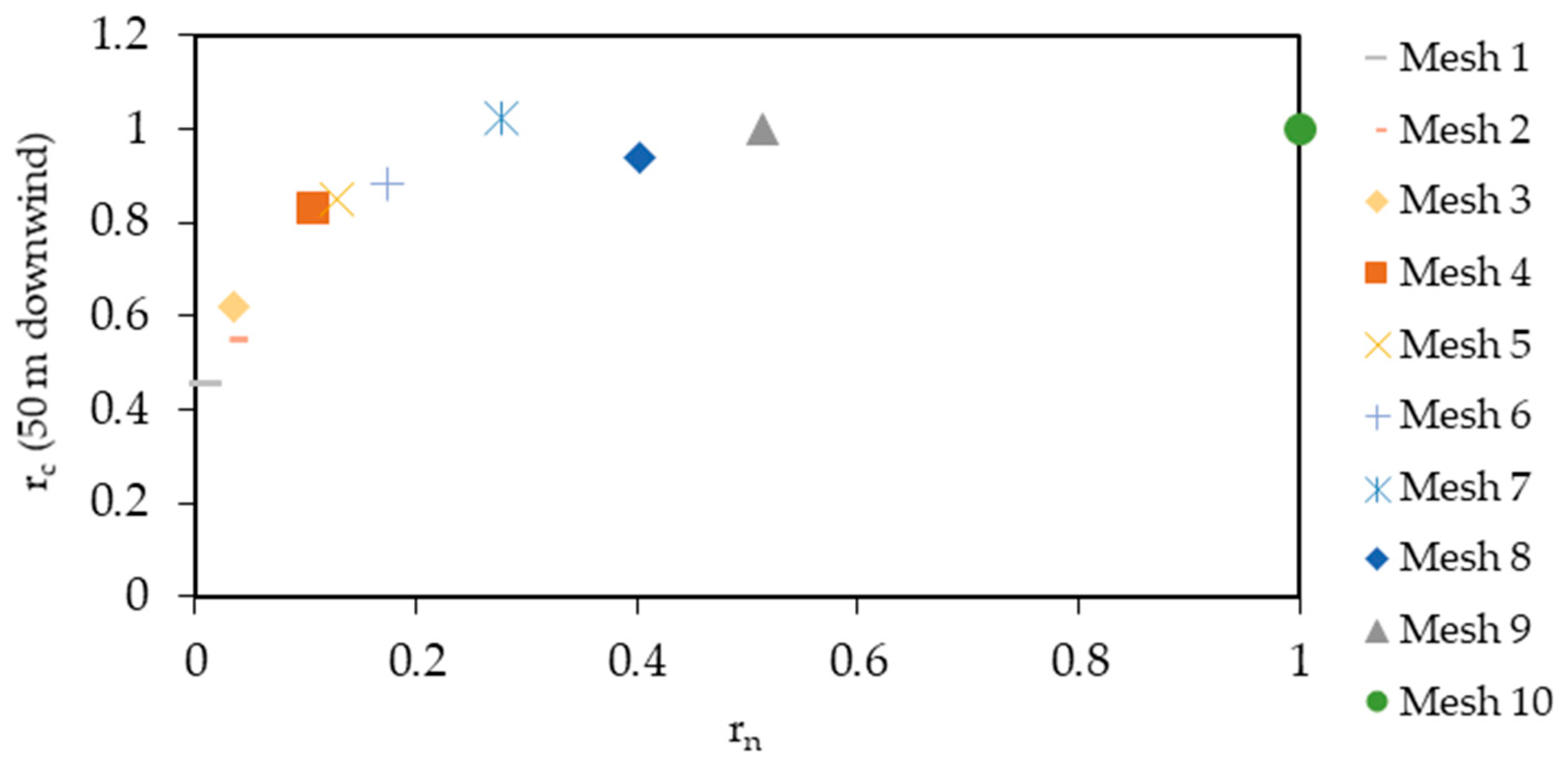
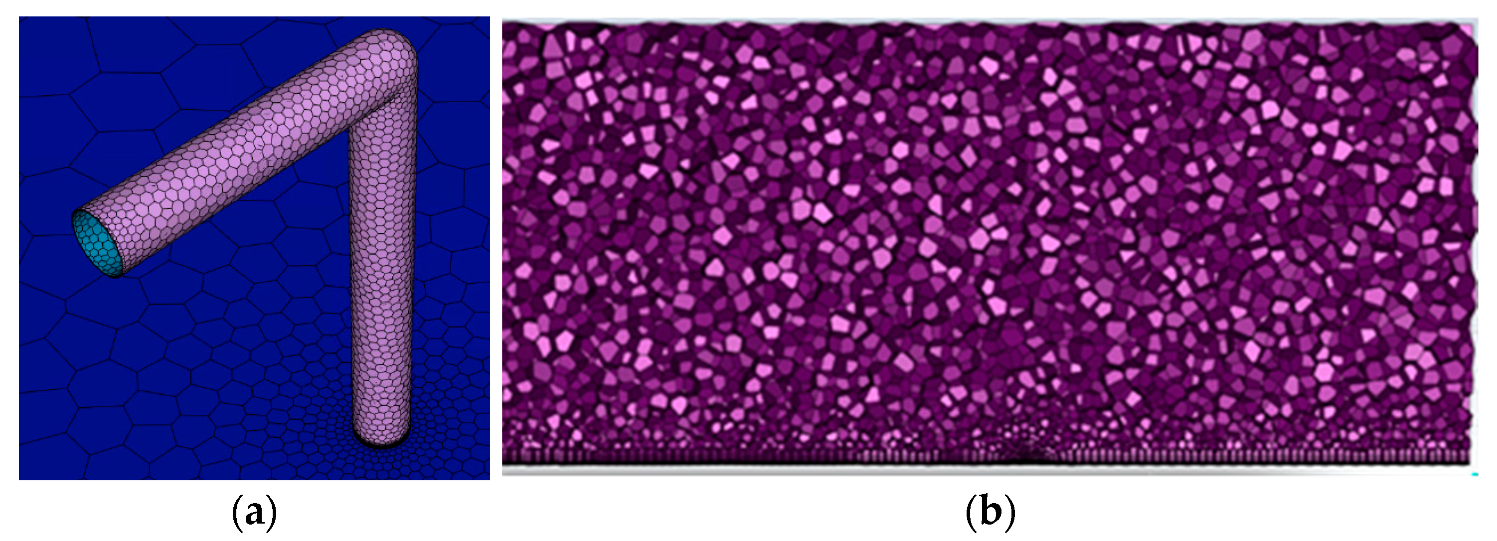
3.1. Mesh Independency

The mesh independence study is performed with the following parameters: the element size, the ground surface sizing, the inflation layers, the use or lack of use of a mesh adaptation function, and the refinement criteria. The ground surface sizing indicates the mesh size at the ground level. The inflation layers, as defined for this case, are a mesh technique that refine the mesh near the ground and gradually increase in size as they move away from the ground. This analysis has accomplished obtaining a mesh that does not affect the results by using a reasonable number of nodes. In other words, there is no appreciable difference in results when further increasing the nodes. The tested mesh characteristics are summarized in Table 2.
The relevance of each parameter (maximum sizing, inflation layers, etc.) is determined by grouping similar meshes. For example, Mesh 9 only differs from Mesh 10 in the refinement criteria. So, the difference in the response is caused by the influence of the studied parameter, which in this case corresponds to the refinement criteria. Comparing both results allows us to interpret the significance of this parameter. Therefore, the concentration and node ratios are plotted (Figure 3). The concentration ratio (rc) is the relationship between the concentration results of a mesh and the mesh with maximum nodes, which in this case is Mesh 10. Similarly, the node ratio (rn) indicates the fraction of mesh nodes over the maximum mesh nodes.
Mesh 10 is used as a reference. Its large number of nodes allows us to assume that it is close to the analytical solution of the model. Mesh 7 (Figure 4) is used to run the simulations as it proves to provide a good balance between accuracy and computational time. Further tests are performed to prove whether y + (non-dimensional distance from the wall [71]) values in the bottom wall have a significant impact on the results. From the later mesh optimization and the tests, it is proven that for this case y + values ranging from 30 to 1000 do not present significantly different results. This may be due to the scarce presence of obstacles and the plain geometry of the system added to the fact that the relevant transport phenomena occur far from the walls.

3.2. Convergence Analysis

The error or imbalance in the solved equations at each iteration is expressed by residuals. Lower residuals imply greater convergence and a more stable solution, and they show how well the present solution meets the governing equations. The continuity equation criterion is set to 10−5. All other residuals are set to converge to at least 10−6 to become acceptable. Figure 5a shows the evolution of those residuals in a simulation. The spikes in convergence correspond to the instances where the mesh is refined. Tracking is also performed in critical zones like the sampling points, where the SO2 concentration is plotted in each iteration to see whether it oscillates significantly at the end of the simulation (Figure 5b). From Figure 5, it can be seen that the mesh refinement has a significant effect on the results.

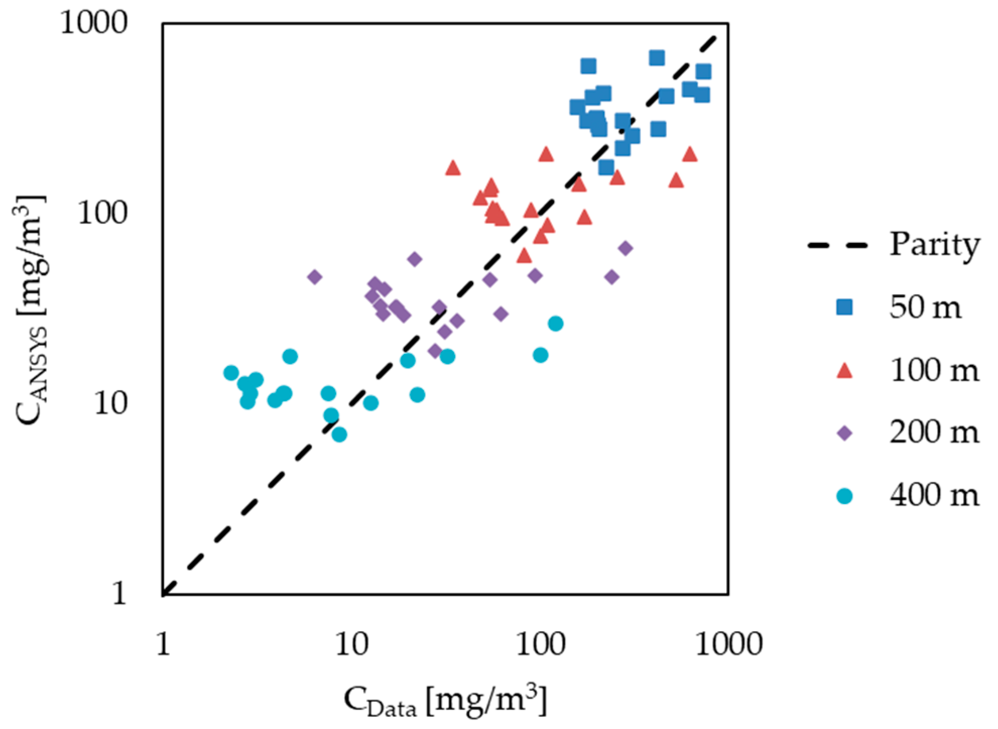
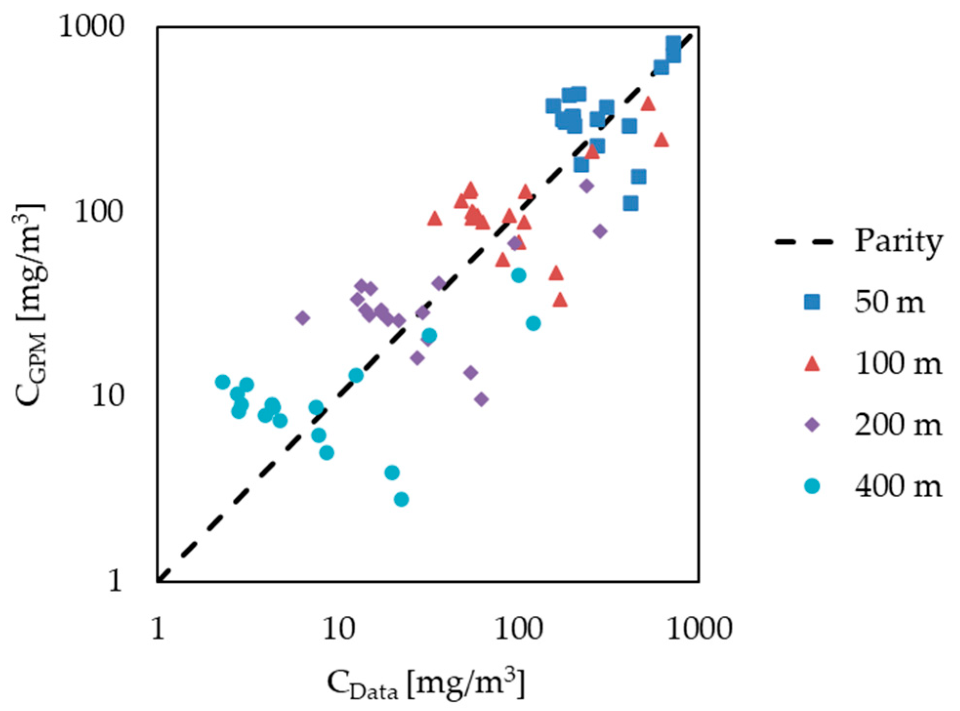
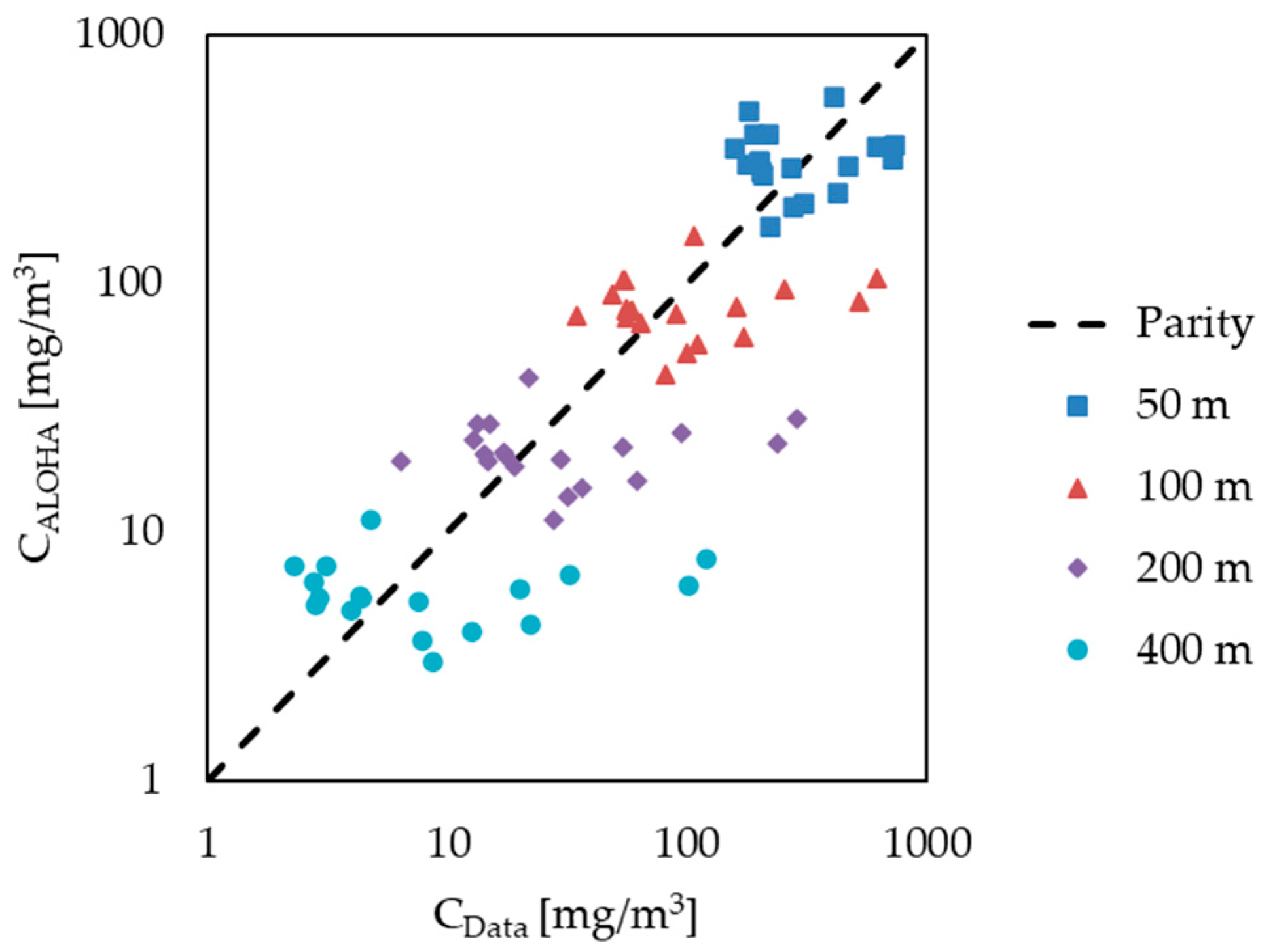
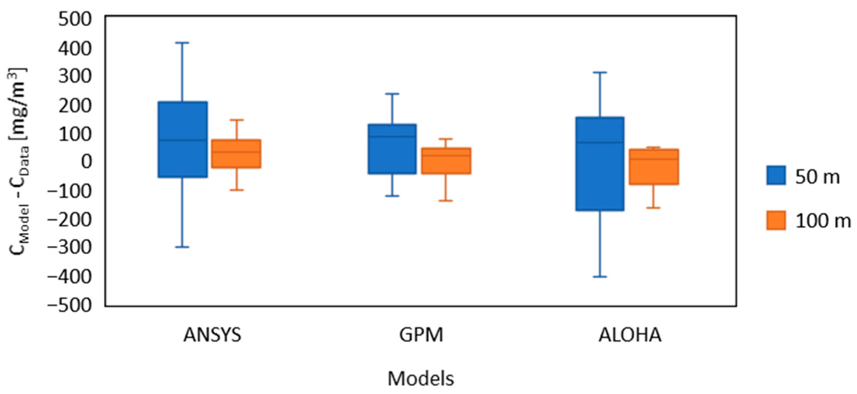
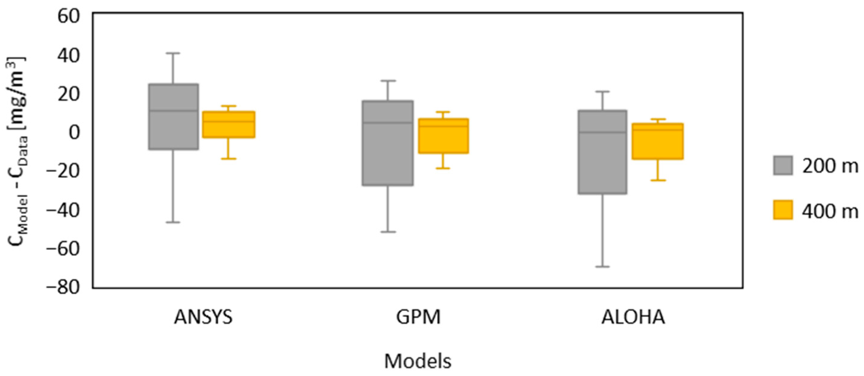
3.3. Comparison Against Experimental Data

The Prairie Grass Project sampling arrays are made up of five concentric arcs located 50, 100, 200, and 400 downwind of the release. The 180-degree arcs are centred on the release and are positioned in the direction of the predominant air velocity. The measurements are taken at a height of 1.5 m. There is also a vertical sampling array providing measurements at nine heights at the 100 m arc: 0.5, 1.0, 1.5, 2.5, 4.5, 7.5, 10.5, 13.5, and 17.5 m [12]. A total of seventy experiments are performed in the Prairie Grass Project, with flow rates between 50 and 100 g/s [59]. SO2 is employed as a tracer. The release pipe has a diameter of two inches (5.08 cm) and a slight right-angle bend at the top to facilitate a horizontal release. The height of the release is 0.46 m for all experiments (Table 1) [12]. As in any empirical experiment, some incidents occur, and they are listed in the Prairie Grass Project volumes. For example, the gas release rate varied over 50% of the average rate in run n° 47 [59]. Olesen et al. categorize these data to be eliminated since they are highly likely to include anomalies [72]. Similarly, this sort of experiment, as well as those with a 1.5 m release height, will not be studied. A total of 19 experiments (releases n° #5, #9, #11, #15, #16, #18, #19, #22, #26, #31–33, #39, #42, #44, #54, #56, #59, and #61) have been selected to be simulated with ANSYS Fluent®, the Gaussian Plume Model (GPM), and ALOHA. Each of these experiments has different parameters that are considered in each simulation. Discrete receptors are placed in the models at the exact same locations where samples are taken in the field experiment. The computational cost of GPM and ALOHA are negligible as results can be obtained almost instantly. Only the know-how time can be considered. For CFD simulations, it takes six hours of computation.
Figure 6 and Figure 7 show how concentration changes with distance and height, using experiment data #61 as an example. In these figures, it is essential to differentiate between experimental and model (GPM, ALOHA, and ANSYS) results. Experimental concentrations represent the peak values within each distance–height range. Model results, however, show concentration at specific points in the downwind direction. This adjustment in experimental concentration is made to minimize the influence of wind fluctuations on the concentration. Since wind changes cannot be replicated because they are not mentioned in the literature, this adjustment also helps to make experimental and model concentration values comparable. The different model profiles mimic the experimental concentration distribution pattern (Figure 6 and Figure 7). Da Silva et al. [53] make the same assessment, comparing the findings of the wind tunnel experiment to the simulations performed with ANSYS Fluent®. ALOHA only provides results at the floor level and therefore is not included in Figure 7.
In both figures, GPM and CFD values are higher than in the experiment. Simulation results being higher than experimental results is a common thing. In the research performed by Habib et al., similar overestimations are found when comparing CFD [73]. They also find that models based on Lagrangian methods can even be more precise than CFD for simple geometry cases. Their research studies concentrations at different distances downwind, and some of the overestimations or underestimations are often due to changes in wind direction, which are not always possible to reproduce in the simulation domains. The present study focuses on steady-state runs, as no transient data are available from the experiment. Since it is not possible to simulate changes in wind direction and velocity, which highly impact the atmospheric dispersion, this may explain the overestimation of vertical concentration. In relation to that, the formula used to describe how wind velocity varies with height [64] may not clearly mimic the real conditions of the experiment. Another possibility is that the criterion used to describe the domain (see Section 2.2) may not be restrictive enough to ensure no spreading restriction in the domain, hindering the vertical dispersion.
ANSYS Fluent® has the benefit of easily visualizing the dispersion phenomena. Planes, lines, or points can be generated across the domain to represent the required variables using various sorts of graphics and charts. As an example, Figure 8 shows the SO2 concentration contour plot at the release point.
Although each case can be examined individually, the model performance is more clearly demonstrated when all simulation results are seen together. The simulation concentration is represented in relation to the experimental concentration. Figure 9, Figure 10 and Figure 11 plot the downwind results of ANSYS Fluent®, GPM, and ALOHA, respectively.
The downwind concentration points of ANSYS Fluent® and GPM are seen to be positioned around the parity line, and visually, the points might be regarded as being evenly dispersed above and below it. In the case of ALOHA, it seems to return slightly lower results than expected. Despite this, the discrepancy between the actual and predicted values in all models is rather large. It is usual to see readings that are twice or half, with the maximum absolute error for all cases and models being around 400 mg/m3 at 50 m. When the measurements are taken diluted away from the release point, this value decreases steadily, reaching 55 mg/m3 at 400 m.
A tendency to overestimate is evident in the ANSYS Fluent® vertical dispersion (Figure 12). Furthermore, because the values decrease with height, a “little” variation in a tiny concentration value reflects a very significant relative difference. To quantify this, we have used the statistical parameter MAE that corresponds to the difference between the modelled and the observed values in terms of absolute value. The MAEs, considering all the measurements at different heights, are 44.4 mg/m3 for ANSYS Fluent® and 30.3 mg/m3 for GPM. As the height increases, the system experiences more turbulence-inducing behaviours that have not been characterized, such as lateral air current entries. These promote contaminant dispersion, and the lack of dispersion found in the simulations is most likely owing to this. At lower heights, the Gaussian model’s concentration predictions usually generate “slight” overestimations (Figure 13). With rising height, there is a trend towards less exact values. The results at the highest elevation (17.5 m) show a significant underestimation. Determining the concentration at high altitudes seems problematic for both ANSYS Fluent® and GPM, although the response is not the same. ALOHA only estimates concentration at ground level; hence, vertical dispersion data are unavailable.
Olesen et al.’s results also show an overestimation in the OML and AERMOD models, especially when the wind velocities are very low [72]. This trend is more accentuated in the AERMOD model. By contrast, the values for the mean concentration profiles are underestimated in the CFD of Da Silva et al.’s study [53]. Despite the possible deviations, CFD adjusts well to reality. This allows for the study of more complex situations that cannot be studied with the other models due to their limitations.

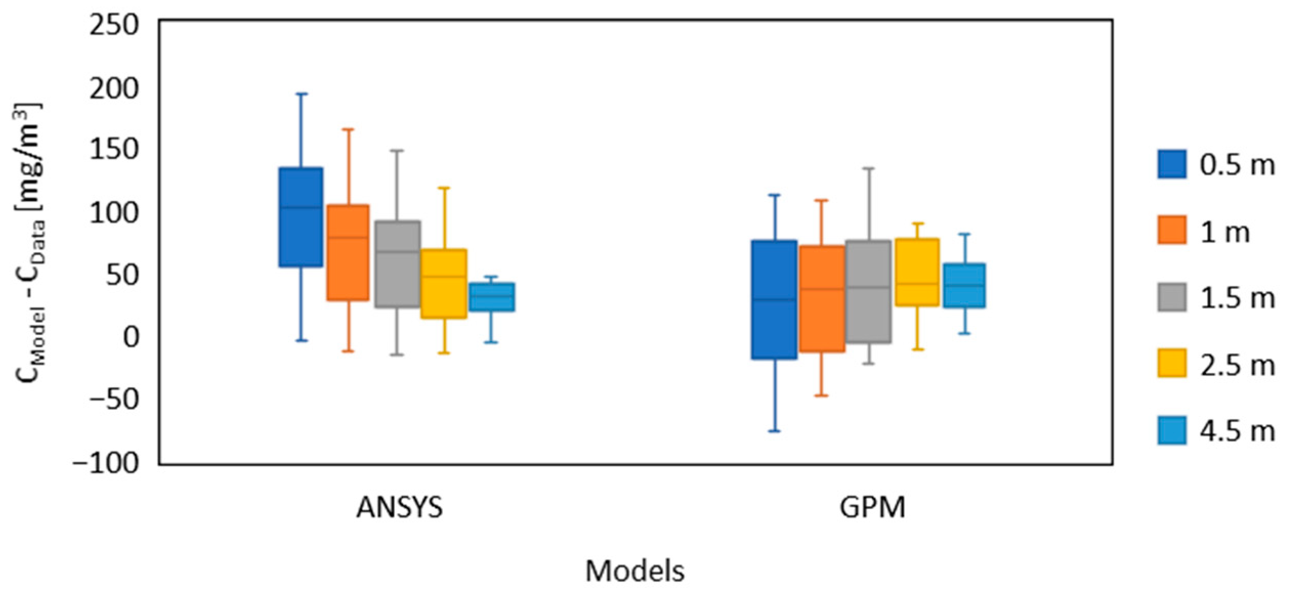
3.4. Model Comparison

The ANSYS Fluent® model’s range of values at 50 m is quite similar to that of ALOHA, with GPM exhibiting less data dispersion (Figure 14). Despite this, the mean concentration variation across models is relatively close: the MAE values for ANSYS Fluent® and ALOHA exhibit a similar deviance from the experimental values (MAEANSYS = 150 mg/m3, MAEALOHA = 167 mg/m3), and GPM produces more accurate results in the emission vicinity (MAEGPM = 108 mg/m3). At the 50 and 100 m downwind distances, the ALOHA model has a larger interquartile range, indicating that the data are less densely clustered.
The extreme errors achieved with the three models at 200 m are comparable, with most of them being between ±40 mg/m3 (Figure 15). ALOHA yields the lowest values (−60 mg/m3). Similar results are observed at 400 m. The 400 m ANSYS Fluent® MAE value is between those from GPM (MAEGPM = 9.4 mg/m3) and ALOHA (MAEALOHA = 6.5 mg/m3).
The overall MAE for downwind dispersion is 61 mg/m3 for ANSYS Fluent®, which is between the GPM and ALOHA values (54 mg/m3 and 63 mg/m3, respectively). For RMSE (Root Mean Square Error), the values for each method are 99 mg/m3, 87 mg/m3, and 107 mg/m3 for the CFD, GPM, and ALOHA models. Finally, the most biased method is CFD, with a Fractional Bias (FB) of 0.16. GPM also overestimates its predictions on average, with an FB of 0.088. ALOHA is the least biased method, with an FB of −0.051. Other statistics are represented in Table 3. The CFD results are of the same magnitude as the ones found in Wang et al. [61]. The equations for these statistical indicators are provided in the Supplementary Materials.
Table 4 represents the FAC2 values of each model at different downwind distances. FAC2 represents the probability (expressed on a unit basis) that the value provided by a model falls between half and twice the experimental value. The FAC2 values for all models increase as the measurement is made closer to the source, which indicates that they decrease in accuracy as we move away from the source. CFD is the model that works best according to this statistical value at closer ranges, which is an expected result since it is a tool often used for close-range gas dispersion.
Even though the errors across the models are of comparable ranges (Figure 16), those provided by ANSYS Fluent® are frequently greater than zero. This suggests an overestimation. Similar phenomena happen with the GPM at heights of 4.5 m or 7.5 m; the model corrects this trend and achieves results closer to the empirical data at heights over 13 m (Figure 17). The vertical towers are located one hundred metres from the emission source, though not at all distances. Consequently, only a portion of the 1.5 m data in the horizontal dispersion are represented in the vertical comparisons (Figure 16).
The average absolute error of ANSYS Fluent® in the vertical dispersion is always higher than GPM. Nevertheless, the MAE values are quite similar, excluding the last two heights. The mean value for all height points is similar: 63 mg/m3 for ANSYS Fluent® and 43 mg/m3 for GPM, which are like those found in the downwind pollutant travel. The RMSE values are higher, 115 mg/m3 for CFD and 95 mg/m3 for GPM, suggesting that some cases have larger errors than in the case of downwind dispersion.
As shown in Table 5, the accuracy and precision of both models, ANSYS and GPM, significantly decreases at 100 m and at different height measurements relative to the results for all distances combined. This suggests that for this case, either the steady-state assumption or other assumptions that both simulations share are not as feasible, or that the conditions in the experiment generate a substantial positive bias, as seen in the FB values of both models. This is better expressed in Table 6, where FB increases as the height of the measurement increases.

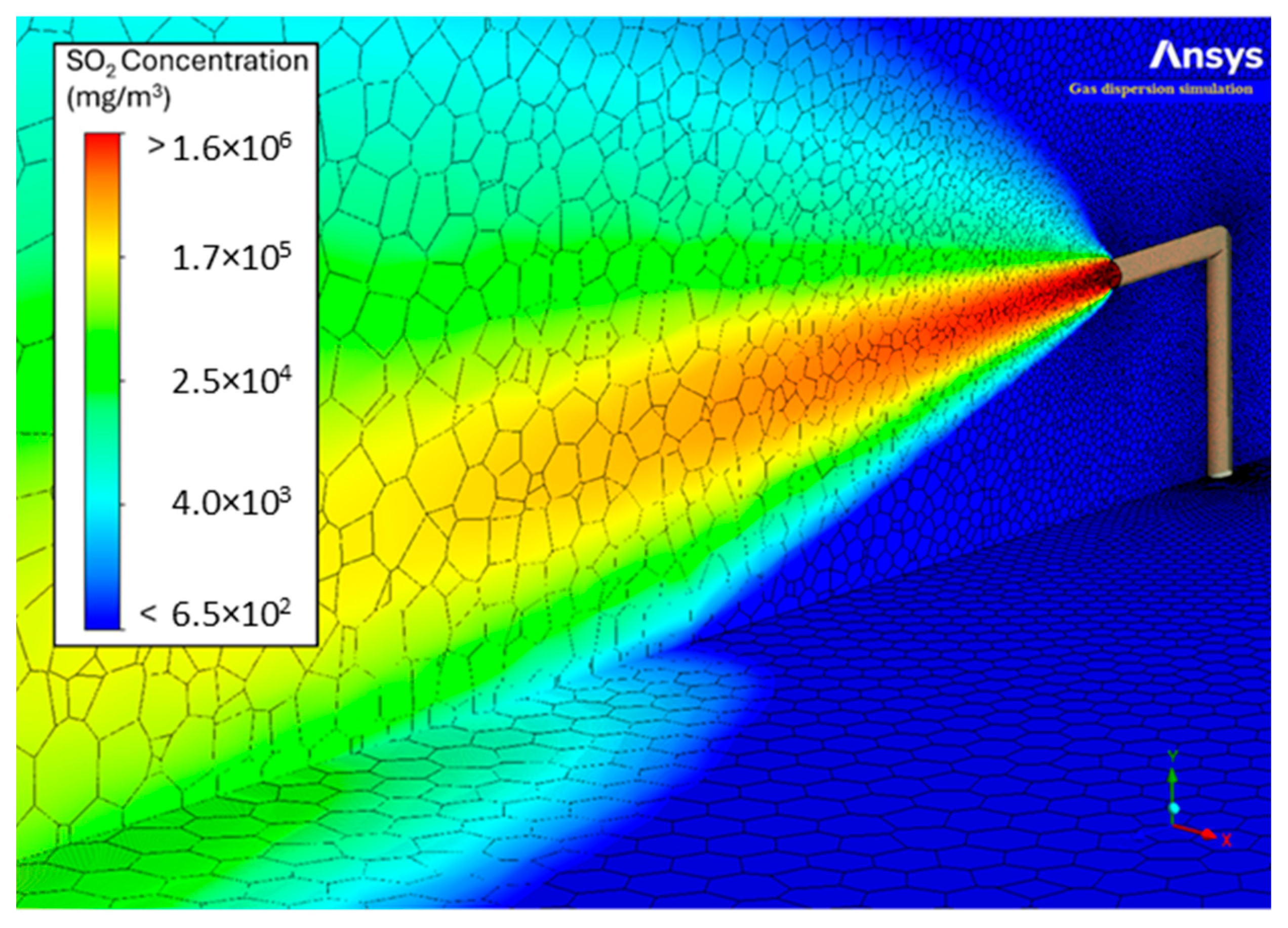
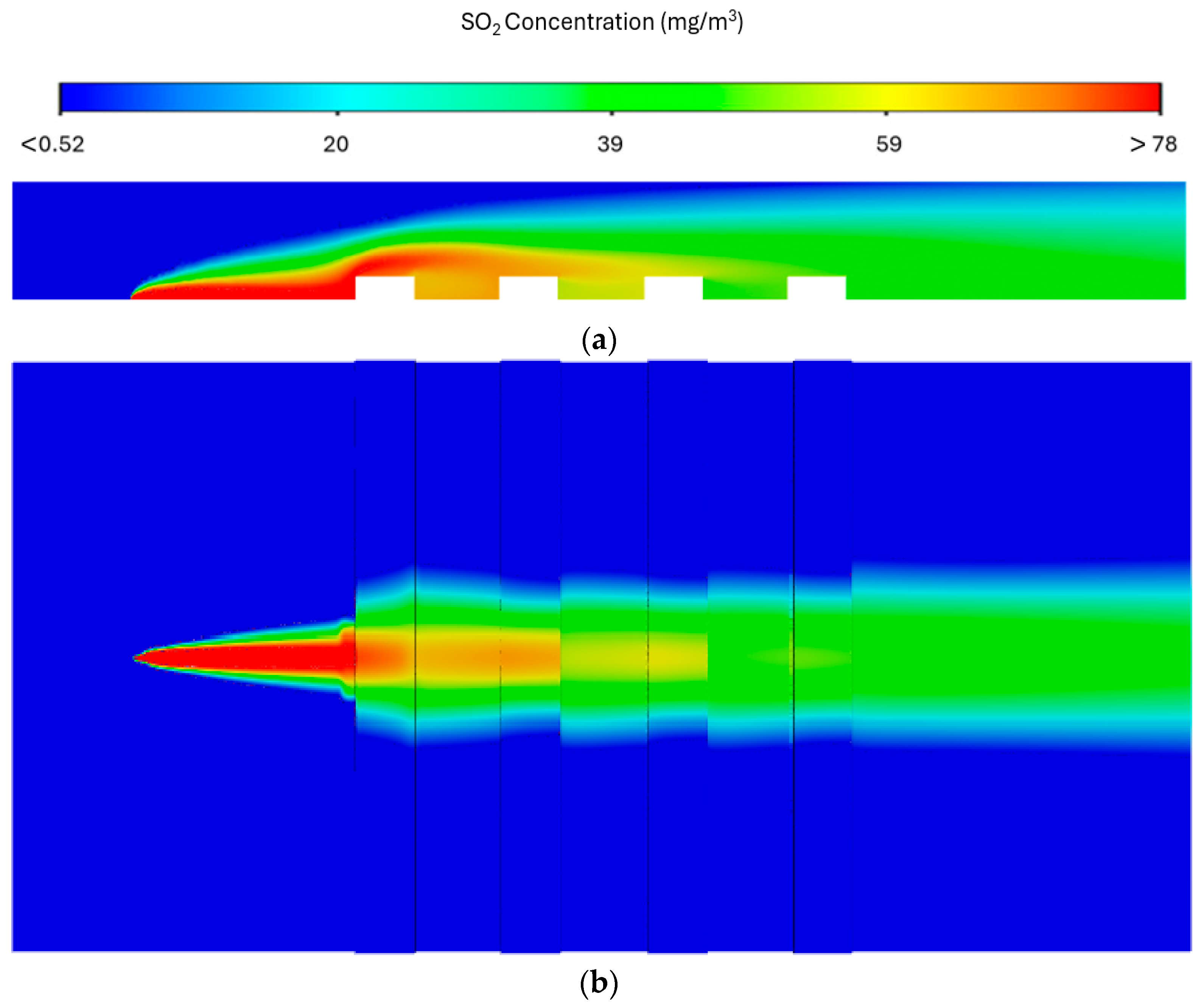
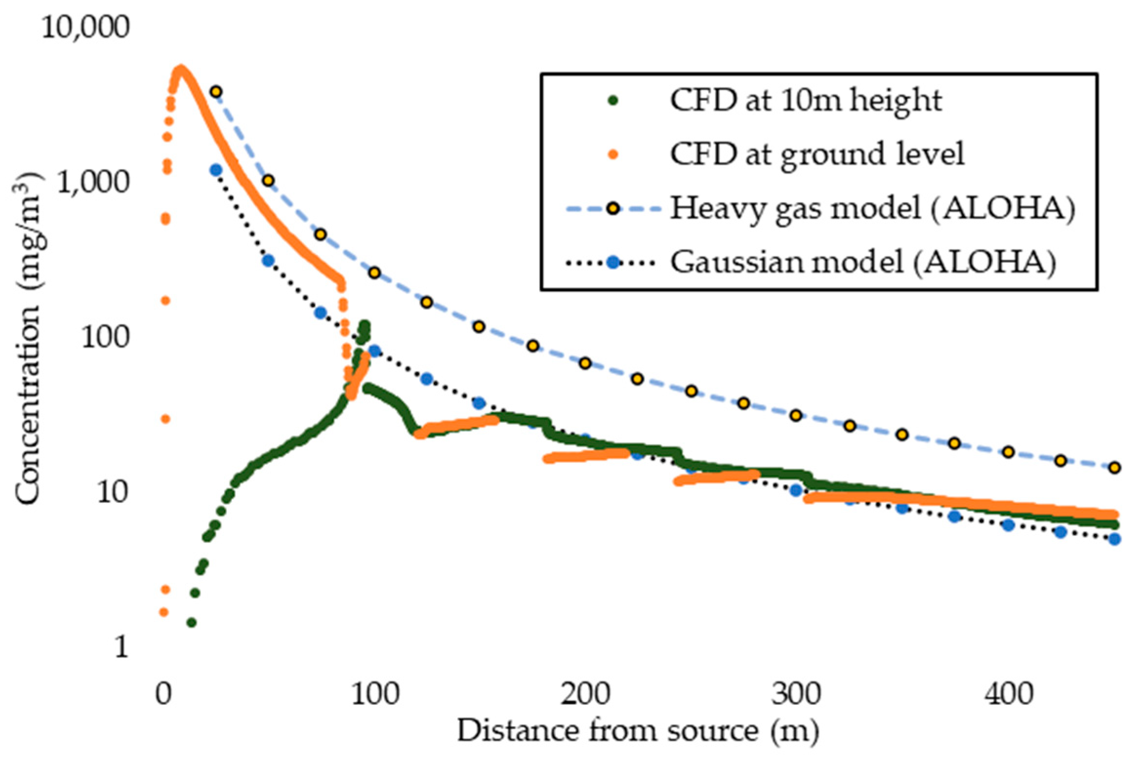
3.5. Results of Gas Dispersion in the Presence of Obstacles

The simulation results display a deflection of the pollutant in the first layer of buildings which considerably decreases the concentration of SO2 at ground level after it passes the obstacles. Figure 18 depicts this phenomenon, showcasing in red 78 mg/m3, which is equivalent to 30 ppm, a value considered to be of high risk by the AEGL-3 [74]. The low (AEGL-1) 0.52 mg/m3 concentrations correspond to 0.2 ppm, a concentration that does not seem to have immediate risks to human health [75].
A comparison between models is shown in Figure 19, where the different models are compared between themselves. Until the first obstacle is encountered, the CFD concentration is between the heavy gas and Gaussian models, as it has a moderately high relative density with respect to air. Once the first obstacle is encountered, the CFD concentration resembles the one seen in Gaussian modelling. Zones where Gaussian and CFD differ are found just after each of the obstacles, as CFD displays a clear decrease in concentration around 125 and 175 m. This is because, in CFD, velocity and turbulence carry the pollutants around, while ALOHA does not take into account the changes in speed and turbulence induced by the obstacles. It is also important to note the concentration at 10 m, that is, at the top of the buildings, which is higher than the concentration on the ground when the air passes over the obstacles. These obstacles act as a protection that decreases ground level pollution, but when the presence of obstacles ceases, the ground concentration returns to being higher than that at 10 m. It can be concluded that ALOHA and CFD can both give similar overall results, but when the interest is on zones near abrupt geometries, CFD gives an edge for understanding the concentration distributions.
This study has shown that CFD may model air pollution spread as accurately as simpler models, like Gaussian Plume Models. However, it is important to recognize that CFD has limits in very simple situations, like the Prairie Grass Project, in which quite long distances are analyzed. In those situations, e.g., flat terrain without obstacles and non-reactive substance dispersion, simpler models give results that are good enough and are faster to calculate. CFD is more complex, needing a detailed mesh and a long calculation time, which may not be necessary for those situations. Therefore, for quick estimations or first looks in simple environments, Gaussian models are still very useful tools. However, it is important to understand that when the situation becomes more complex, like in the simulations of gas dispersion in the presence of obstacles proposed in this paper, Gaussian models become less accurate. In those cases, the detailed simulations from CFD give a more realistic and dependable picture of how air pollution spreads.

4. Conclusions

The accurate prediction of pollutant dispersion is essential to determining the impact of these atmospheric pollutants on human health. SO2, which is a pollutant generated by the combustion of sulphur-containing fuels, is used as a tracer in this research for comparing the dispersion results of different models: ALOHA, GPM, and CFD. The CFD’s advantages are clearly seen near the emission source, in complex terrains, or in its capacity to consider pollutant reactions. However, the Prairie Grass scenario measures concentrations up to 800 m away from the emission source, the emission is performed in a quite flat open terrain, and it uses a low reactive pollutant. So, it may be said that this studied scenario “benefits” GPM and ALOHA. Moreover, the GPM uses Prairie Grass experiments to fit this model, ALOHA works well at distances up to 2 km, and both are unable to introduce pollutant reactions. Despite this, the results show that CFD is a valuable tool for emission analysis, performing comparably to established models like GPM and ALOHA, while offering greater versatility across a wider range of scenarios.
When comparing the models, the CFD (ANSYS Fluent®) shows a similar accuracy to GPM and ALOHA for downwind dispersion predictions near the ground, but CFD overestimates the concentration towards the top of the plume. Interestingly, GPM occasionally displays similar overestimation tendencies, which may validate the correct configuration of our CFD model for predicting atmospheric gas dispersion in open terrain. Despite that, it must be considered that the lack of data results in an inaccurate representation of the atmospheric conditions, reducing vertical dispersion. CFD predictions are expected to be improved with a clear and wide atmospheric database throughout the emission, which is able to reproduce the real-world atmospheric conditions that affect dispersion.
In terms of the time needed to obtain the results, this CFD setup takes roughly six hours to compute, whereas GPM or ALOHA take just a few minutes. So, just looking at the required time, GPM or ALOHA are better for basic cases and in situations where you are running out of time, e.g., emergencies. Otherwise, CFD has the potential to adapt itself to a particular scenario: terrain, obstacles, substance, or reaction, as clearly seen in the case of the presence of an obstacle.
The results of this research can contribute to generating tools to analyze the impact of industrial emissions on the air quality of a region. These modelling-based tools can be powerful resources for environmental managers across various industries (e.g., petrochemistry, wastewater plants, mining, smelters), helping them to adopt appropriate decisions to reduce the impact of their activity on air quality, favouring sustainable development. Similarly, these tools can effectively handle the risk situations associated with uncontrolled or unexpected emissions into the atmosphere.

Supplementary Materials

The following supporting information can be downloaded at: https://www.mdpi.com/article/10.3390/su17104403/s1, Table S1: Concentration values (kmol/m3) for the different meshes tested at various downwind distances.

Author Contributions

Conceptualization, A.E.P.P., J.B. and J.L.; methodology, R.C.; software, R.C. and C.T.F.; validation, R.C.; formal analysis, R.C. and C.T.F.; investigation, R.C. and C.T.F.; resources, A.E.P.P., J.B. and J.L.; data curation, C.T.F.; writing—original draft preparation, R.C. and C.T.F.; writing—review and editing, A.E.P.P., J.B. and R.A.A.; visualization, R.C. and C.T.F.; supervision, A.E.P.P., J.B. and R.A.A.; project administration, A.E.P.P. and J.B.; funding acquisition, A.E.P.P., J.B. and J.L. All authors have read and agreed to the published version of the manuscript.

Funding

This research was funded by the Agency for Management of University and Research Grants (“Agència de Gestió d’Ajuts Universitaris i de Recerca”), grant number 2022 DI 00024, and by the Mir Puig Private Foundation (“Fundació Privada Mir Puig”).

Institutional Review Board Statement

Not applicable.

Informed Consent Statement

Not applicable.

Data Availability Statement

Data will be made available on request.

Conflicts of Interest

Author Raúl Arasa Agudo was employed by the Meteosim. The remaining authors declare that the research was conducted in the absence of any commercial or financial relationships that could be construed as a potential conflict of interest.

Abbreviations

The following abbreviations are used in this manuscript:
ALOHAAreal Location of Hazardous Atmosphere
CFDComputational Fluid Dynamics
CRLCell Refine Level
FAC2Fraction of the Prediction Within a Factor of 2 of the Observations
GPMGaussian Plume Model
MAEMean Absolute Error
FBFractional Bias
NMSENormalized Mean Square Error
RMSERoot Mean Square Error
SO2Sulphur Dioxide
SSTShear Stress Transport

References

  1. EEA. How Air Pollution Affects Our Health; European Environment Agency: Copenhagen, Denmark, 2024; Available online: https://www.eea.europa.eu/en/topics/in-depth/air-pollution/eow-it-affects-our-health (accessed on 18 December 2024).
  2. WHO. Air Pollution: The Invisible Health Threat; World Health Organization: Geneva, Switzerland, 2024; Available online: https://www.who.int/news-room/feature-stories/detail/air-pollution--the-invisible-health-threat (accessed on 18 December 2024).
  3. Newby, D.E.; Manucci, P.M.; Grethe, S.T.; Baccarelli, A.A.; Brook, R.D.; Donaldson, K.; Forastiere, F.; Franchini, M.; Franco, O.H.; Graham, I.; et al. Expert Position Paper on Air Pollution and Cardiovascular Disease. Eur. Heart J. 2015, 36, 83–93. [Google Scholar] [CrossRef] [PubMed]
  4. Crutzen, P.J. New Directions: The Growing Urban Heat and Pollution Island Effect-Impact on Chemistry and Climate. Atmos. Environ. 2004, 38, 3539–3540. [Google Scholar] [CrossRef]
  5. Salvador, A.; Arasa, R.; Codina, B. Aeolian Dust Forecast in Arid and Semiarid Regions of Peru and Chile and Their Contribution over Particulate Matter Concentration. J. Geosci. Environ. Prot. 2016, 4, 128–152. [Google Scholar] [CrossRef]
  6. Directive-EU-2024/2881-EN-EUR-Lex. Available online: https://eur-lex.europa.eu/eli/dir/2024/2881/oj (accessed on 28 January 2025).
  7. Lacome, J.-M.; Leroy, G.; Joubert, L.; Truchot, B. Harmonisation in Atmospheric Dispersion Modelling Approaches to Assess Toxic Consequences in the Neighbourhood of Industrial Facilities. Atmosphere 2023, 14, 1605. [Google Scholar] [CrossRef]
  8. Li, D.; Liu, G.; Mao, Z. Leak Detection and Localization in Multi-Grid Space Using Improved Gaussian Plume Model. Sensors 2023, 23, 6209. [Google Scholar] [CrossRef]
  9. Leelőssy, Á.; Molnár, F.; Izsák, F.; Havasi, Á.; Lagzi, I.; Mészáros, R. Dispersion Modeling of Air Pollutants in the Atmosphere: A Review. Cent. Eur. J. Geosci. 2014, 6, 257–278. [Google Scholar] [CrossRef]
  10. Chang, J.C.; Hanna, S.R. Modelers’ Data Archive. A Collection of Atmospgeric Transport and Dispersion Data Sets. In Proceedings of the 16th AMS Conference on Air Pollution Meteorology, Atlanta, GA, USA, 17 January 2010. [Google Scholar]
  11. George Mason University. Field Data Sets. Available online: http://camp.cos.gmu.edu/FieldDatasetInventory.htm (accessed on 4 February 2023).
  12. Irwin, J.S. Project Prairie Grass—Atmospheric Transport and Diffusion Data Archive. Available online: https://www.harmo.org/jsirwin/PrairieGrassDiscussion.html (accessed on 4 February 2023).
  13. Lu, J.; Huang, M.; Wu, W.; Wei, Y.; Liu, C. Application and Improvement of the Particle Swarm Optimization Algorithm in Source-Term Estimations for Hazardous Release. Atmosphere 2023, 14, 1168. [Google Scholar] [CrossRef]
  14. Venkatram, A.; Thé, J. Introduction to Gaussian Plume Models. In Air Quality Modeling—Theories, Methodologies, Computational Techniques, and Available Databases and Software; Zannetti, P., Ed.; The EnviroComp Institute and the Air & Waste Management Association: New York, NY, USA, 2003; Volume 1, pp. 185–207. [Google Scholar]
  15. Ahmed, S.K.; Kabir, G.; Khan, M.S.A. Development of a Consequence-Based Decision-Making Framework for Natural Gas Transmission Pipeline. Innov. Infrastruct. Solut. 2022, 7, 307. [Google Scholar] [CrossRef]
  16. Ren, Y.; Zhang, G.; Zheng, J.; Miao, H. An Integrated Solution for Nuclear Power Plant On-Site Optimal Evacuation Path Planning Based on Atmospheric Dispersion and Dose Model. Sustainability 2024, 16, 2458. [Google Scholar] [CrossRef]
  17. National Oceanic and Atmospheric Administration (NOAA). ALOHA® (Areal Locations of Hazardous Atmospheres) 5.4.4: Technical Documentation; NOAA: Seattle, WA, USA, 2013. [Google Scholar]
  18. Terzioglu, L.; Iskender, H. Modeling the Consequences of Gas Leakage and Explosion Fire in Liquefied Petroleum Gas Storage Tank in Istanbul Technical University, Maslak Campus. Process Saf. Prog. 2021, 40, 319–326. [Google Scholar] [CrossRef]
  19. Micallef, A.; Micallef, C. The Gaussian Plume Model Equation for Atmospheric Dispersion Corrected for Multiple Reflections at Parallel Boundaries: A Mathematical Rewriting of the Model and Some Numerical Testing. Sci 2024, 6, 48. [Google Scholar] [CrossRef]
  20. Boikos, C.; Rapkos, N.; Ioannidis, G.; Oppo, S.; Armengaud, A.; Siamidis, P.; Tsegas, G.; Ntziachristos, L. Factors affecting pedestrian-level ship pollution in port areas: CFD in the service of policy-making. Build. Environ. 2024, 258, 111594. [Google Scholar] [CrossRef]
  21. Pakchotanon, P.; Veawab, A.; Aroonwilas, A.; Sema, T. Atmospheric Dispersion of Gaseous Amine Emitted from Absorption-Based Carbon Capture Plants in Saskatchewan, Canada. Energies 2022, 15, 1221. [Google Scholar] [CrossRef]
  22. Whiteman, C.D.; Hoch, S.W.; Horel, J.D.; Charland, A. Relationship between Particulate Air Pollution and Meteorological Variables in Utah’s Salt Lake Valley. Atmos. Environ. 2014, 94, 742–753. [Google Scholar] [CrossRef]
  23. Yuval; Tritscher, T.; Raz, R.; Levi, Y.; Levy, I.; Broday, D.M. Emissions vs. Turbulence and Atmospheric Stability: A Study of Their Relative Importance in Determining Air Pollutant Concentrations. Sci. Total Environ. 2020, 733, 139300. [Google Scholar] [CrossRef]
  24. Udina, M.; Rosa Soler, M.; Arasa, R. Effects of Nocturnal Thermal Circulation and Boundary Layer Structure on Pollutant Dispersion in Complex Terrain Areas: A Case Study. Int. J. Environ. Pollut. 2012, 48, 47–59. [Google Scholar] [CrossRef]
  25. Soler, M.R.; Arasa, R.; Merino, M.; Olid, M.; Ortega, S. Modelling Local Sea-Breeze Flow and Associated Dispersion Patterns Over a Coastal Area in North-East Spain: A Case Study. Bound. Layer Meteorol. 2011, 140, 37–56. [Google Scholar] [CrossRef]
  26. Chemel, C.; Burns, P. Pollutant Dispersion in a Developing Valley Cold-Air Pool. Bound. Layer Meteorol. 2015, 154, 391–408. [Google Scholar] [CrossRef]
  27. Iskender, H. Risk Assessment for an Acetone Storage Tank in a Chemical Plant in Istanbul, Turkey: Simulation of Dangerous Scenarios. Process Saf. Prog. 2021, 40, 234–239. [Google Scholar] [CrossRef]
  28. Ahmad, M.A.; Rashid, Z.A.; El-Harbawi, M.; Al-Awadi, A.S. High-Pressure Methanol Synthesis Case Study: Safety and Environmental Impact Assessment Using Consequence Analysis. Int. J. Environ. Sci. Technol. 2022, 19, 8555–8572. [Google Scholar] [CrossRef]
  29. Sánchez-Pérez, J.F.; García-Ros, G.; Castro, E. Simultaneous Determination of the Position, Release Time and Mass Release Rate of an Unknown Gas Emission Source in Short-Term Emissions by Inverse Problem. Chem. Eng. J. 2022, 445, 136782. [Google Scholar] [CrossRef]
  30. Shojaee Barjoee, S.; Elmi, M.R.; Talebi Varaoon, V.; Keykhosravi, S.S.; Karimi, F. Hazards of Toluene Storage Tanks in a Petrochemical Plant: Modeling Effects, Consequence Analysis, and Comparison of Two Modeling Programs. Environ. Sci. Pollut. Res. 2022, 29, 4587–4615. [Google Scholar] [CrossRef] [PubMed]
  31. Mouilleau, Y.; Champassith, A. CFD Simulations of Atmospheric Gas Dispersion Using the Fire Dynamics Simulator (FDS). J. Loss Prev. Process Ind. 2009, 22, 316–323. [Google Scholar] [CrossRef]
  32. Węsierski, T.; Piec, R.; Majder-łopatka, M.; Król, B.; Gawroński, W.; Kwiatkowski, M. Hazards Generated by an LNG Road Tanker Leak: Field Investigation of Vapour Propagation Under Class B Conditions of Atmospheric Stability. Energies 2021, 14, 8483. [Google Scholar] [CrossRef]
  33. Zhang, Z.; Lv, J.; Li, W.; Long, J.; Wang, S.; Tan, D.; Yin, Z. Performance and Emission Evaluation of a Marine Diesel Engine Fueled with Natural Gas Ignited by Biodiesel-Diesel Blended Fuel. Energy 2022, 256, 124662. [Google Scholar] [CrossRef]
  34. New Zealand. Ministry for the Environment. National Institute of Water and Atmospheric Research (N.Z.); Aurora Pacific (Firm); Earth Tech (Firm) Good Practice Guide for Atmospheric Dispersion Modelling; Ministry for the Environment: Wellington, New Zealand, 2004; ISBN 0478189419. [Google Scholar]
  35. Gant, S.E.; Tucker, H. Computational Fluid Dynamics (CFD) Modelling of Atmospheric Dispersion for Land-Use Planning around Major Hazards Sites in Great Britain. J. Loss Prev. Process Ind. 2018, 54, 340–345. [Google Scholar] [CrossRef]
  36. Wang, X.; Bao, W.; Huang, X.; Wang, X.; Du, F.; Wang, D.; Wang, B. A CFD Model Based on Wet Deposition of Large-Scale Natural Draft Cooling Tower. Rev. Int. De Contam. Ambient. 2019, 35, 23–32. [Google Scholar] [CrossRef]
  37. Ansys. Engineering Simulation Software. Available online: https://www.ansys.com/ (accessed on 9 February 2023).
  38. Gianfelice, M.; Aboshosha, H.; Ghazal, T. Real-Time Wind Predictions for Safe Drone Flights in Toronto. Results Eng. 2022, 15, 100534. [Google Scholar] [CrossRef]
  39. Oliver, A.; Arasa, R.; Pérez-Foguet, A.; Ángeles González, M. Simulating Large Emitters Using CMAQ and a Local Scale Finite Element Model. Analysis of the Surroundings of Barcelona. Int. J. Environ. Pollut. 2017, 62, 155–183. [Google Scholar] [CrossRef]
  40. Vasudevan, M.; Pilla, F.; McNabola, A. Enhancing ventilation in street canyons using adjustable roof-level wind flow de-flectors. Energy Built Environ. 2025, 6, 201–218. [Google Scholar] [CrossRef]
  41. Gao, S.; Chen, Q.; Chen, Y.; Ye, J.; Chen, L. A Study on Street Tree Planting Strategy in Pingtan Island Based on Road Wind Environment Simulation. Sustainability 2024, 16, 6252. [Google Scholar] [CrossRef]
  42. Shen, Z.; Lang, J.; Li, M.; Mao, S.; Hu, F.; Xuan, B. Impact of Inlet Boundary Number and Locations on Gas Diffusion and Flow in a Typical Chemical Industrial Park near Uneven Terrain. Process Saf. Environ. Prot. 2022, 159, 281–293. [Google Scholar] [CrossRef]
  43. Schleder, A.M.; Martins, M.R. Experimental Data and CFD Performance for CO2 Cloud Dispersion Analysis. J. Loss Prev. Process Ind. 2016, 43, 688–699. [Google Scholar] [CrossRef]
  44. Escarti-Guillem, M.S.; Hoyas, S.; García-Raffi, L.M. Rocket Plume URANS Simulation Using OpenFOAM. Results Eng. 2019, 4, 100056. [Google Scholar] [CrossRef]
  45. Synylo, K.; Krupko, A.; Zaporozhets, O.; Makarenko, R. CFD Simulation of Exhaust Gases Jet from Aircraft Engine. Energy 2020, 213, 118610. [Google Scholar] [CrossRef]
  46. San José, R.; Pérez, J.L.; Pérez, L.; Gonzalez Barras, R.M. Effects of Climate Change on the Health of Citizens Modelling Urban Weather and Air Pollution. Energy 2018, 165, 53–62. [Google Scholar] [CrossRef]
  47. Hanjalić, K.; Kenjereš, S. Dynamic Simulation of Pollutant Dispersion Over Complex Urban Terrains: A Tool for Sustainable Development, Control and Management. Energy 2005, 30, 1481–1497. [Google Scholar] [CrossRef]
  48. Wójtowicz-Wróbel, A.; Kania, O.; Kocewiak, K.; Wójtowicz, R.; Dzierwa, P.; Trojan, M. Thermal-Flow Calculations for a Thermal Waste Treatment Plant and CFD Modelling of the Spread of Gases in the Context of Urban Structures. Energy 2023, 263, 125952. [Google Scholar] [CrossRef]
  49. Xin, B.; Dang, W.; Yan, X.; Yu, J.; Bai, Y. Dispersion Characteristics and Hazard Area Prediction of Mixed Natural Gas Based on Wind Tunnel Experiments and Risk Theory. Process Saf. Environ. Prot. 2021, 152, 278–290. [Google Scholar] [CrossRef]
  50. Mehdi, M.; Panin, M.P. Use of Computational Fluid Dynamics Tools to Calculate the Dispersion of Gas and Aerosol Emissions in Conditions of a Complex Terrain. Nucl. Energy Technol. 2021, 7, 21–26. [Google Scholar] [CrossRef]
  51. Akhter, M.N.; Ali, M.E.; Rahman, M.M.; Hossain, M.N.; Molla, M.M. Simulation of Air Pollution Dispersion in Dhaka City Street Canyon. AIP Adv. 2021, 11, 065022. [Google Scholar] [CrossRef]
  52. Clements, D.; Coburn, M.; Cox, S.J.; Bulot, F.M.J.; Xie, Z.-T.; Vanderwel, C. Comparing Large-Eddy Simulation and Gaussian Plume Model to Sensor Measurements of an Urban Smoke Plume. Atmosphere 2024, 15, 1089. [Google Scholar] [CrossRef]
  53. Da Silva, F.T.; Costa Reis, N., Jr.; Meri Santos, J.; Valentim Goulart, E.; Engel de Alvarez, C. The Impact of Urban Block Typology on Pollutant Dispersion. J. Wind Eng. Ind. Aerodyn. 2021, 210, 104524. [Google Scholar] [CrossRef]
  54. Da Silva, F.T.; Reis, N.C.; Santos, J.M.; Goulart, E.V.; de Alvarez, C.E. Influence of Urban Form on Air Quality: The Combined Effect of Block Typology and Urban Planning Indices on City Breathability. Sci. Total Environ. 2022, 814, 152670. [Google Scholar] [CrossRef]
  55. Sharma, H.; Vaidya, U.; Ganapathysubramanian, B. Contaminant Source Identification from Finite Sensor Data: Perron–Frobenius Operator and Bayesian Inference. Energies 2021, 14, 6729. [Google Scholar] [CrossRef]
  56. Wang, R.; Zhang, Z.; Gong, D. Simulation Study on Gas Leakage Law and Early Warning in a Utility Tunnel. Sustainability 2023, 15, 15375. [Google Scholar] [CrossRef]
  57. Scire, J.S.; Strimaitis, D.G.; Yamartino, R.J. A User’s Guide for the CALPUFF Dispersion Model; Earth Technology Inc.: Cedar City, UT, USA, 2000. [Google Scholar]
  58. Jittra, N.; Pinthong, N.; Thepanondh, S. Performance Evaluation of AERMOD and CALPUFF Air Dispersion Models in Industrial Complex Area. Air Soil Water Res. 2015, 8, 87–95. [Google Scholar] [CrossRef]
  59. Morton, L. Barad Project Prairie Grass; Air Force Cambridge Research Laboratories: Bedford, UK, 1958; Volume I and II. [Google Scholar]
  60. Zhang, B.; Chen, G.M. Quantitative Risk Analysis of Toxic Gas Release Caused Poisoning—A CFD and Dose-Response Model Combined Approach. Process Saf. Environ. Prot. 2010, 88, 253–262. [Google Scholar] [CrossRef]
  61. Wang, J.; You, R. Evaluating different categories of turbulence models for calculating air pollutant dispersion in street canyons with generic and real urban layouts. J. Wind Eng. Ind. Aerodyn. 2024, 255, 105948. [Google Scholar] [CrossRef]
  62. Ansys Fluent Theory Guide; ANSYS, Inc.: Canonsburg, PA, USA, 2022.
  63. Guevara Luna, F.A.; Guevara Luna, M.A.; Belalcázar Cerón, L.C. CFD modeling and validation of tracer gas dispersion to evaluate self-pollution in School Buses. Asian J. Atmos. Environ. 2019, 13, 1–10. [Google Scholar] [CrossRef]
  64. OpenFOAM: User Guide: AtmBoundaryLayer. Available online: https://www.openfoam.com/documentation/guides/latest/doc/guide-bcs-inlet-atm-atmBoundaryLayer.html (accessed on 21 September 2022).
  65. Martin, D.O. Comment On “The Change of Concentration Standard Deviations with Distance”. J. Air Pollut. Control Assoc. 1976, 26, 145–147. [Google Scholar] [CrossRef]
  66. Air Resources Laboratory. READY Tools—Pasquill Stability Classes. Available online: https://www.ready.noaa.gov/READYpgclass.php (accessed on 15 January 2023).
  67. ALOHA. Office of Environment, Health, Safety & Security. Department of Energy. Available online: https://www.energy.gov/ehss/aloha (accessed on 29 January 2023).
  68. U.S. Department of Veterans Affairs. ALOHA (Areal Locations of Hazardous Atmospheres). Available online: https://www.oit.va.gov/Services/TRM/ToolPage.aspx?tid=9015 (accessed on 29 January 2023).
  69. Ermak, D.L. User’s Manual for SLAB: An Atmospheric Dispersion Model for Denser-Than-Air-Releases; Lawrence Livermore National Laboratory (LLNL): Livermore, CA, USA, 1990. [Google Scholar] [CrossRef]
  70. World Meteorological Organization. Guide to Meteorological Instruments and Methods of Observation, 6th ed.; Secretariat of the World Meteorological Organization: Geneva, Switzerland, 1996. [Google Scholar]
  71. Schlichting, H.; Gersten, K. Boundary-Layer Theory, 8th ed.; Springer: Berlin/Heidelberg, Germany, 2000; pp. 522–530. [Google Scholar] [CrossRef]
  72. Olesen, H.R.; Berkowicz, R.; Løfstrøm, P. Evaluation of OML and AERMOD. In Proceedings of the International Conference on Harmonisation within Atmospheric Dispersion Modelling for Regulatory Purposes, Cambridge, UK, 2–5 July 2007. [Google Scholar]
  73. Habib, A.; Schalau, B.; Schmidt, D. Comparing Tools of Varying Complexity for Calculating the Gas Dispersion. Process Saf. Environ. Prot. 2014, 92, 305–310. [Google Scholar] [CrossRef]
  74. National Research Council (U.S.). Acute Exposure Guideline Levels for Selected Airborne Chemicals. Volume 8. 9-Sulfur Dioxide; National Academy Press: Washington, DC, USA, 2010; ISBN 0309145163. [Google Scholar]
  75. INSST. Documentación Toxicológica Para El Establecimiento Del Límite de Exposición Profesional Del Dióxido de Azufre; INSST: Madrid, Spain, 2014. (In Spanish) [Google Scholar]
Figure 1. Description of the simulation domain: (a) boundaries; (b) elbow emission flue geometry.
Sustainability 17 04403 g001
Figure 2. Domain with obstacles (orange). The emission is produced in the location of the coordinate axis.
Sustainability 17 04403 g002
Figure 3. Mesh independence study results for concentrations at 50 m downwind from the source.
Sustainability 17 04403 g003
Figure 4. Resulting mesh: (a) surface mesh around the emission nozzle, an exact reproduction of the one used in the experiment [59]; (b) side view of a cut mesh in the downwind plane.
Sustainability 17 04403 g004
Figure 5. Convergence analysis: (a) residuals of a typical simulation with mesh refinement; (b) tracking of SO2 concentration at various distances from the emission at each of the 600 iterations.
Sustainability 17 04403 g005
Figure 6. Release #61—Sulphur dioxide concentration distribution downwind at 1.5 m height.
Sustainability 17 04403 g006
Figure 7. Release #61—Sulphur dioxide concentration height distribution at 100 m distance.
Sustainability 17 04403 g007
Figure 8. Example of SO2 concentration plot in ANSYS Fluent®. The high values of SO2 at the emission source are of almost pure SO2 gas.
Sustainability 17 04403 g008
Figure 9. ANSYS Fluent® findings at different downwind distances in relation to experimental data.
Sustainability 17 04403 g009
Figure 10. Gaussian Plume Model downwind findings in relation to experimental data.
Sustainability 17 04403 g010
Figure 11. ALOHA findings in relation to experimental data and downwind dispersion.
Sustainability 17 04403 g011
Figure 12. Vertical dispersion results in ANSYS Fluent®.
Sustainability 17 04403 g012
Figure 13. GPM outcomes at different heights.
Sustainability 17 04403 g013
Figure 14. Box-and-whisker diagram for concentrations at 50 and 100 m downwind.
Sustainability 17 04403 g014
Figure 15. Box-and-whisker diagram for 200 and 400 m downwind concentrations.
Sustainability 17 04403 g015
Figure 16. Box-and-whisker diagram for heights less than 5 m.
Sustainability 17 04403 g016
Figure 17. Box-and-whisker diagram for heights from 7.5 m to 17.5 m.
Sustainability 17 04403 g017
Figure 18. Simulation results of an emission with obstacles: (a) side view; (b) top view of the lowest level concentration (floor or rooftop).
Sustainability 17 04403 g018
Figure 19. Comparison between ALOHA Gaussian model, ALOHA heavy gas model, and CFD at different heights considering obstacles.
Sustainability 17 04403 g019
Table 1. Simulating domain configurations.
ParameterValueUnit
DomainLength500m
Width250m
Height50m
Prairie Grass
emission pipe [59]
Height0.46m
Diameter0.0508m
Table 2. Mesh characteristics.
Mesh
Name
Max Sizing
[m]
Ground Surface Sizing [m]Inflation
Layers
Refinement
Criteria
Nodes
(106)
Mesh 155--1.1
Mesh 233--4.3
Mesh 333-10−64.6
Mesh 42.5615-13.7
Mesh 52.56110-16.5
Mesh 62.56120-22.3
Mesh 7 *2.5611010−735.6
Mesh 82.560.510-51.7
Mesh 92.560.51010−666.0
Mesh 102.560.51010−7128.7
* Chosen option, as discussed below.
Table 3. Model comparison statistics for concentration estimations versus experimental results on average for all downwind measurements at 1.5 m height.
MethodMAE (mg/m3)RMSE (mg/m3)FBFAC2NMSE
ANSYS CFD61990.160.640.58
GPM54870.0880.600.49
ALOHA63107−0.0510.610.85
Table 4. FAC2 values at different distances downwind at 1.5 m height.
Method50 m100 m200 m400 m
ANSYS CFD0.840.760.560.41
GPM0.740.650.610.41
ALOHA0.740.820.560.35
Table 5. Model comparison statistics for concentration estimations versus experimental results on average for all different heights at 100 m downwind.
MethodMAE (mg/m3)RMSE (mg/m3)FBFAC2NMSE
ANSYS CFD631150.270.192.74
GPM43950.150.422.05
Table 6. FB and NMSE for ANYS and GPM methods at different heights.
Measurement HeightANSYS CFDGPM
FBNMSEFBNMSE
0.5 m0.161.8−0.0861.6
1 m0.111.80.0091.3
1.5 m0.101.50.0810.9
2.5 m0.310.90.410.5
4.5 m0.720.80.801.0
7.5 m1.021.70.911.4
10.5 m1.071.80.601.0
13.5 m1.031.50.0770.68
17.5 m0.931.3−0.702.4
Disclaimer/Publisher’s Note: The statements, opinions and data contained in all publications are solely those of the individual author(s) and contributor(s) and not of MDPI and/or the editor(s). MDPI and/or the editor(s) disclaim responsibility for any injury to people or property resulting from any ideas, methods, instructions or products referred to in the content.

