
Projecting Daily Maximum Temperature Using an Enhanced Hybrid Downscaling Approach in Fujian Province, China

Abstract
1. Introduction
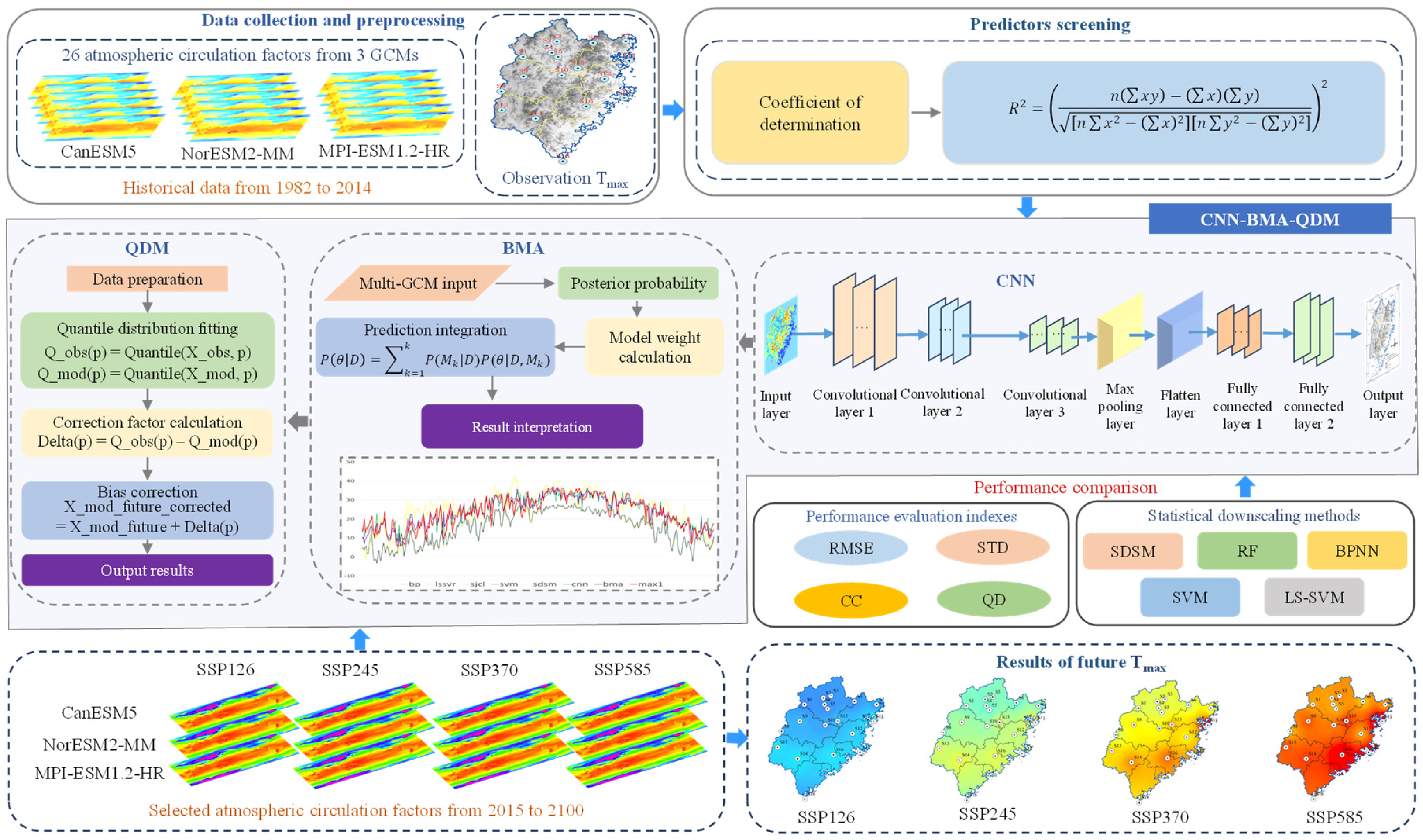
2. Methods
2.1. Statistical Downscaling Model
2.1.1. CNN
2.1.2. SDSM
2.1.3. RF
2.1.4. SVM
2.1.5. LS-SVM
2.1.6. BPNN
2.2. BMA
2.3. QDM
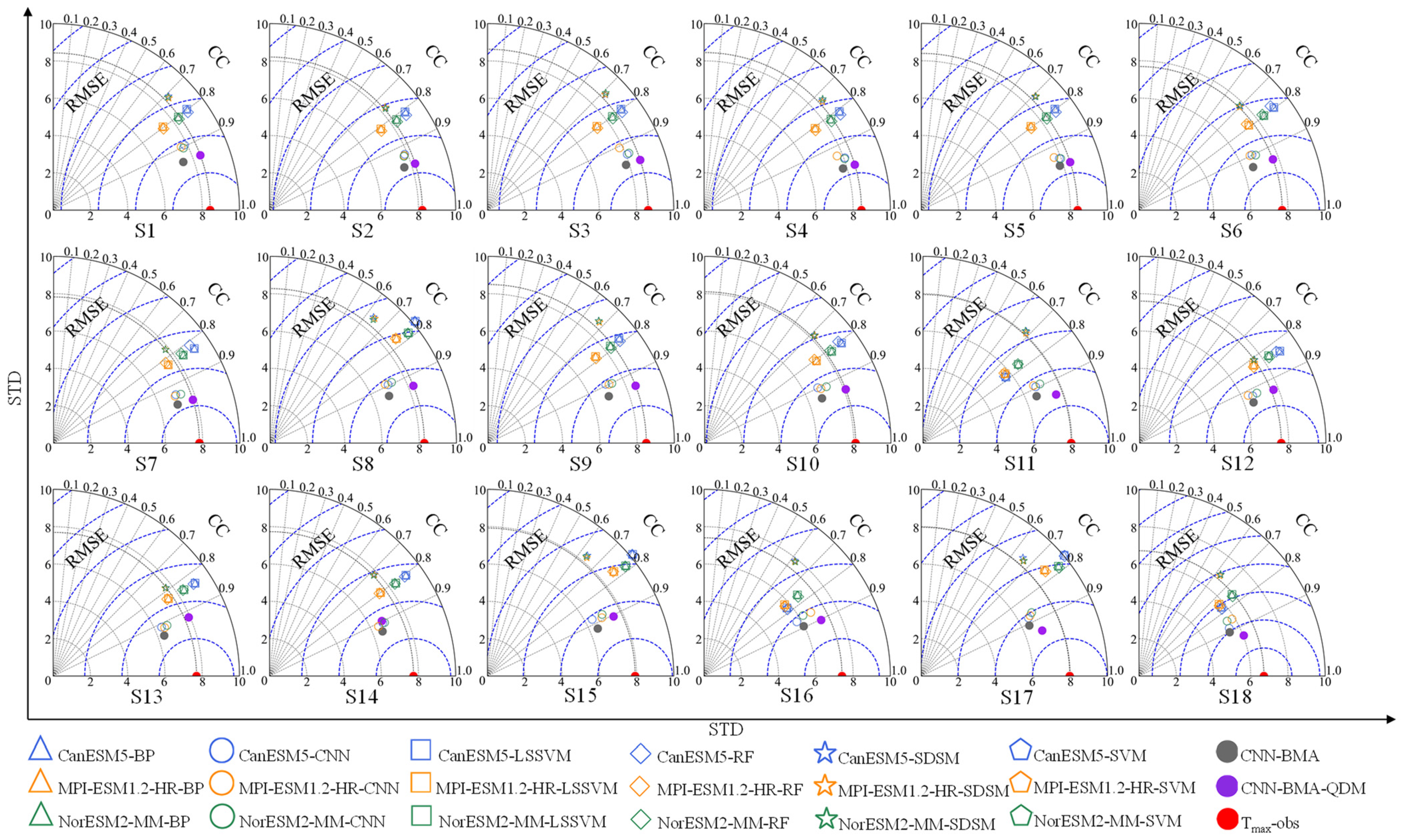
2.4. Performance Evaluation Metrics
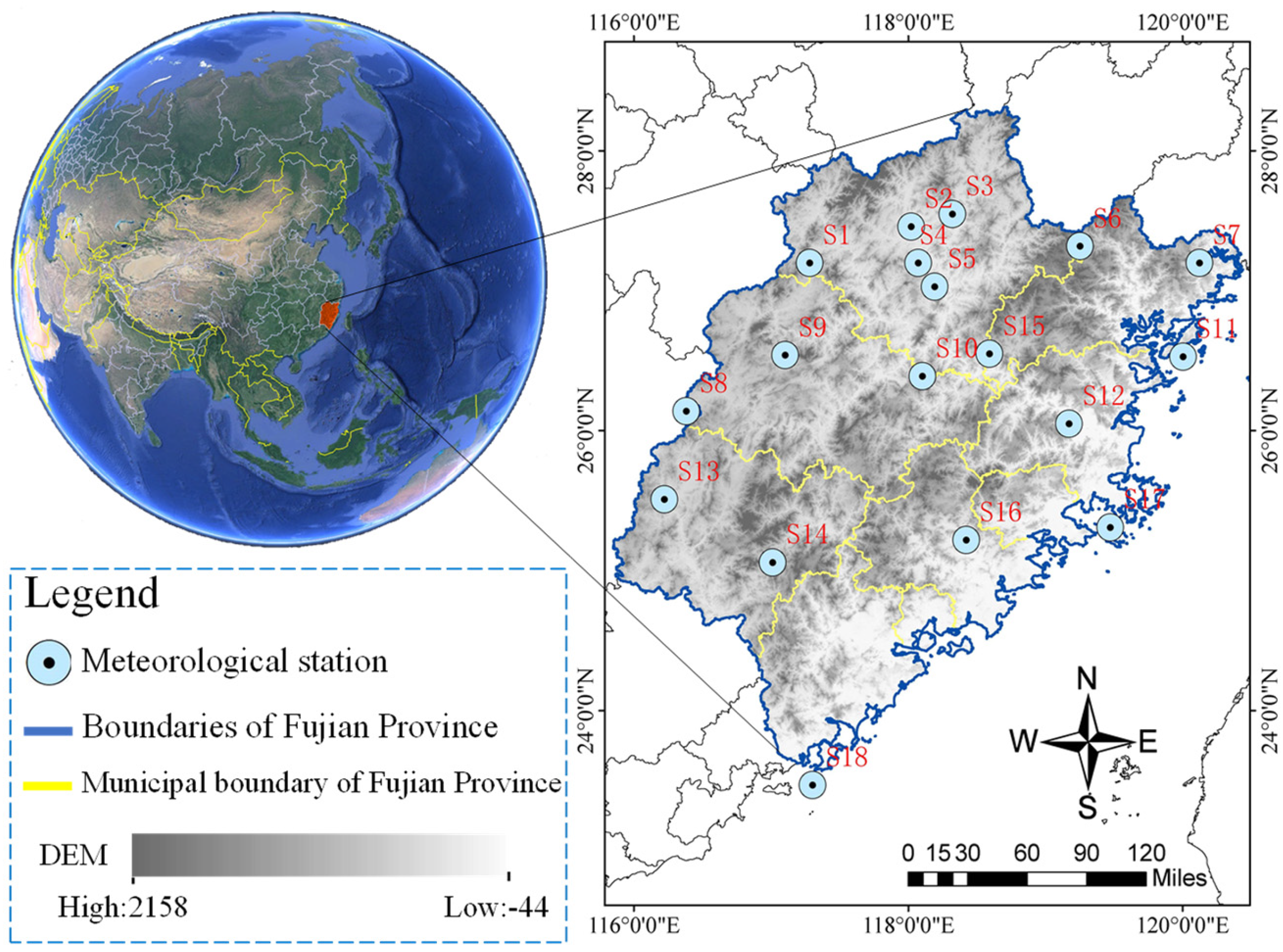
3. Study Area and Data
3.1. Study Area
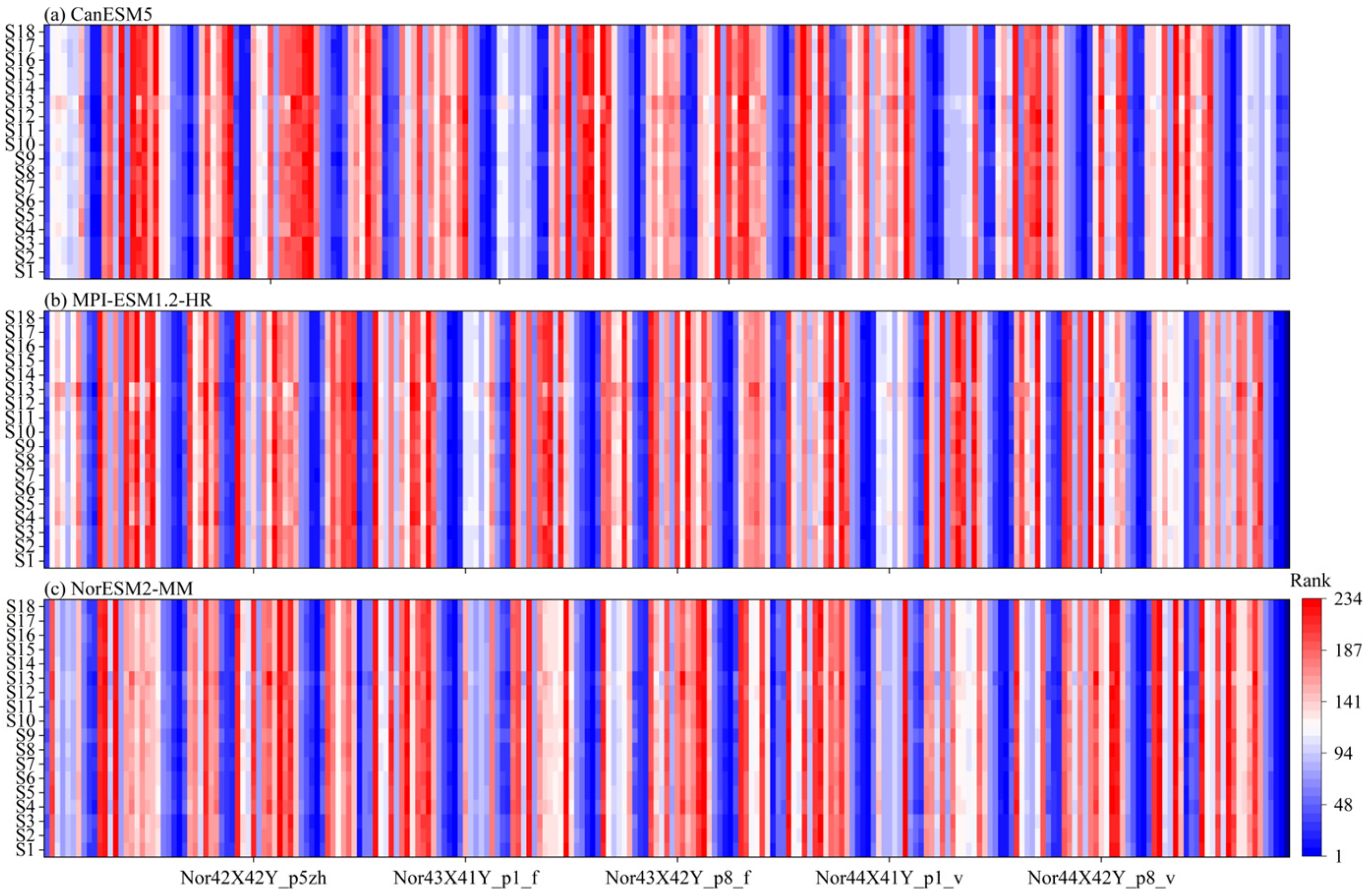
3.2. Data Sources and Preprocessing
4. Results
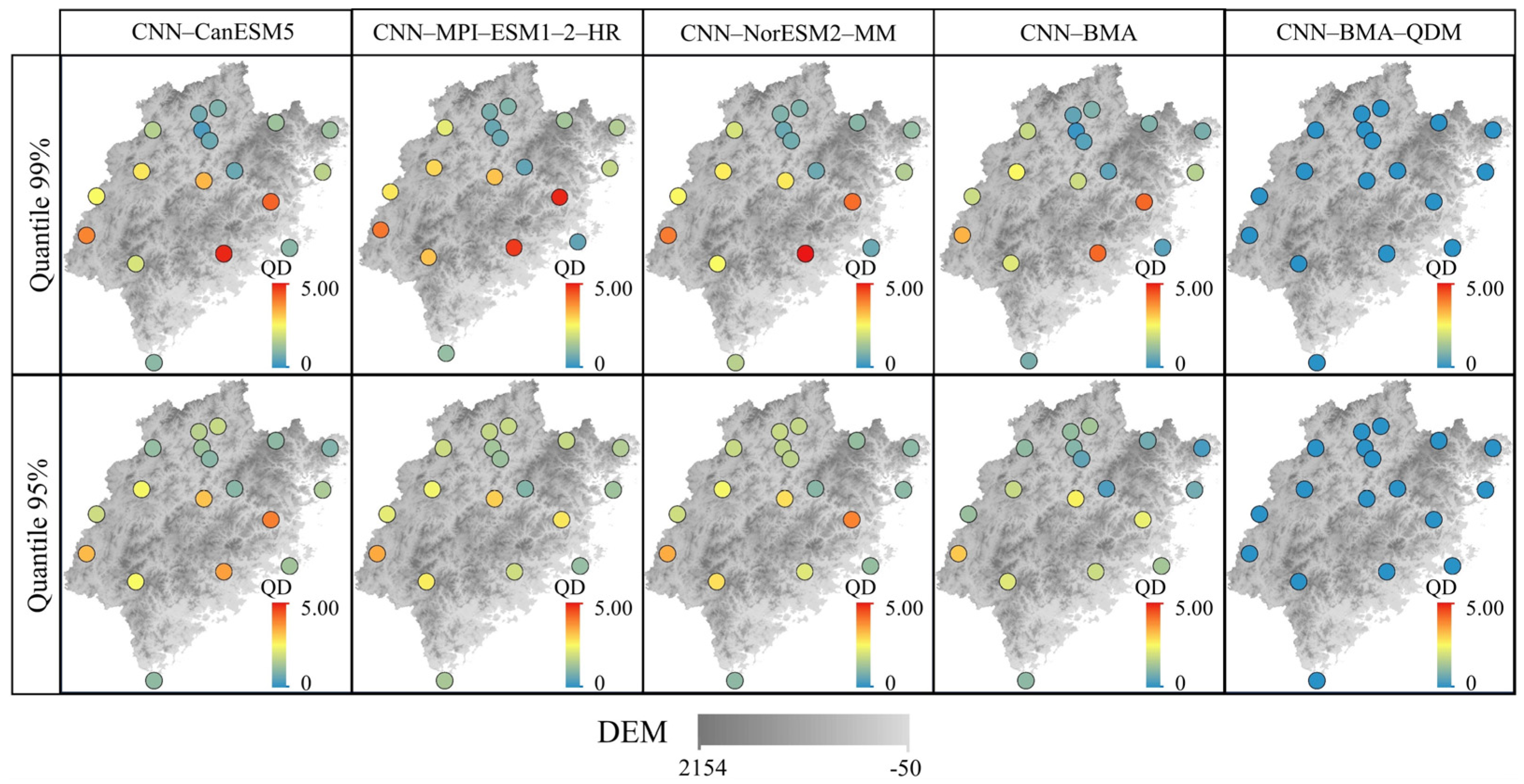
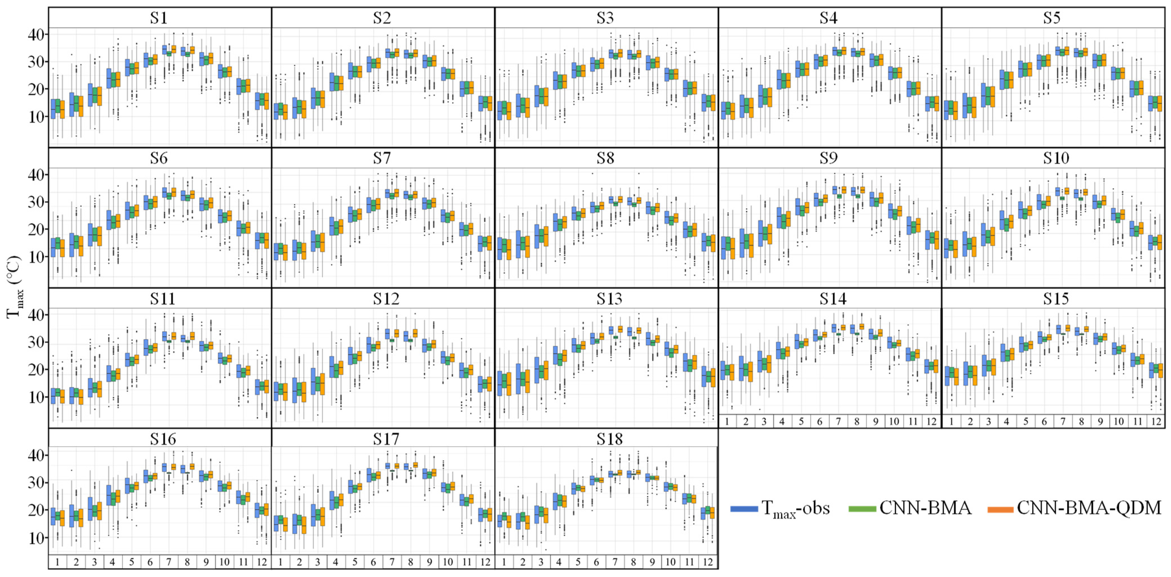
4.1. The Performance of CNN-BMA-QDM
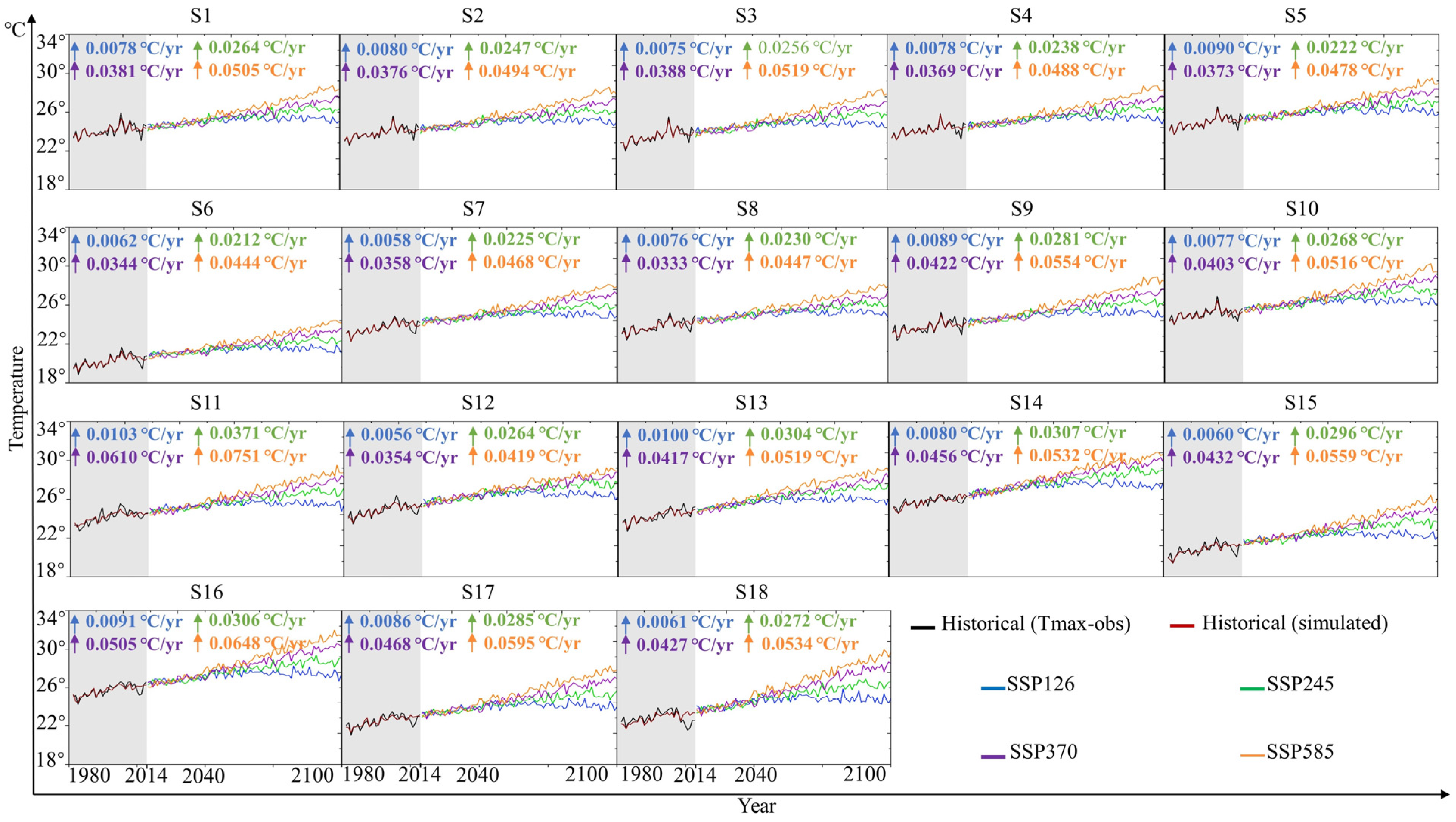
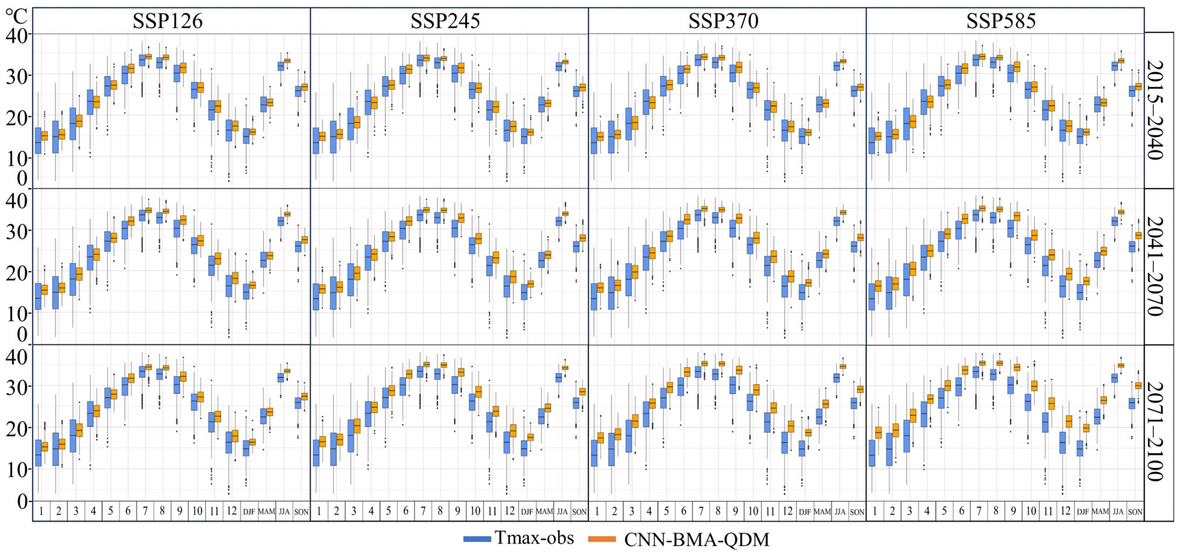
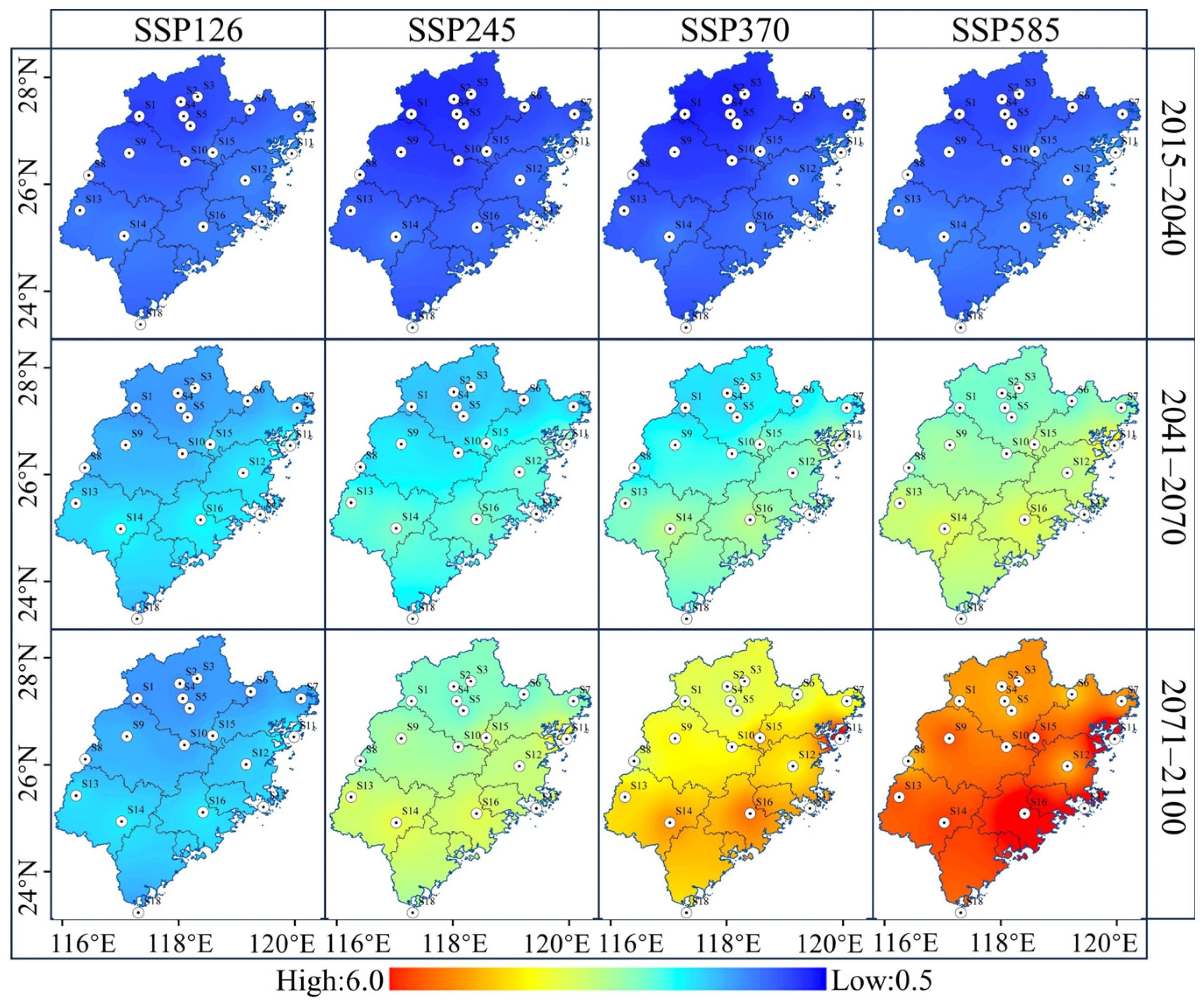
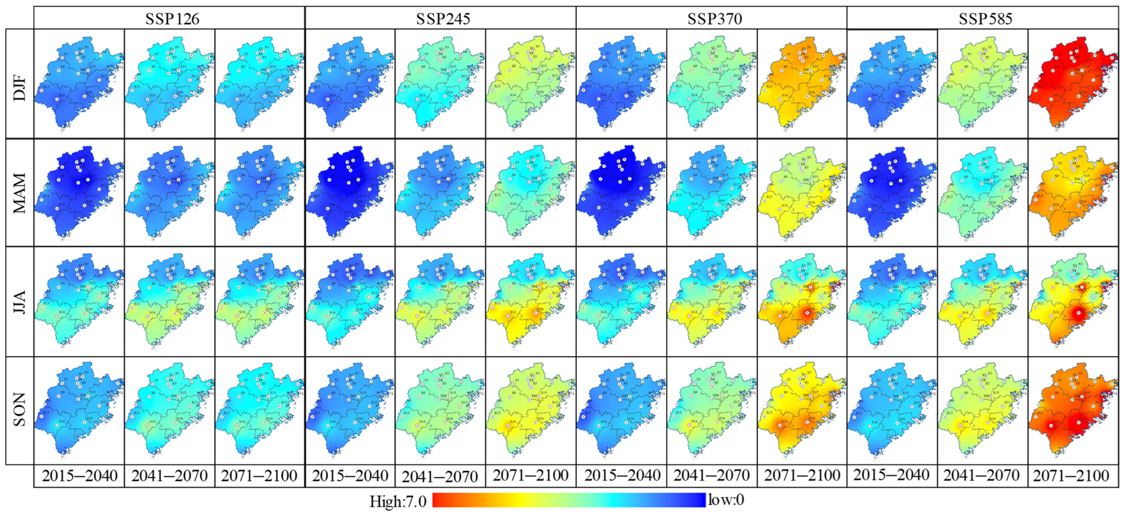
4.2. Spatiotemporal Evolution of Projected Tmax
5. Discussion
6. Conclusions
Supplementary Materials
Author Contributions
Funding
Institutional Review Board Statement
Informed Consent Statement
Data Availability Statement
Acknowledgments
Conflicts of Interest
References
- IPCC. Climate Change 2022: Impacts, Adaptation, and Vulnerability. In Contribution of Working Group II to the Sixth Assessment Report of the Intergovernmental Panel on Climate Change; IPCC: Geneva, Switzerland, 2022. [Google Scholar]
- Hai, Z.; Perlman, R.L. Extreme weather events and the politics of climate change attribution. Sci. Adv. 2022, 8, eabo2190. [Google Scholar] [CrossRef] [PubMed]
- Li, D.; Belitz, M.; Campbell, L.; Guralnick, R. Extreme weather events have strong but different impacts on plant and insect phenology. Nat. Clim. Change 2025, 15, 321–328. [Google Scholar] [CrossRef]
- Khraishah, H.; Alahmad, B.; Ostergard, R.L., Jr.; AlAshqar, A.; Albaghdadi, M.; Vellanki, N.; Chowdhury, M.M.; Al-Kindi, S.G.; Zanobetti, A.; Gasparrini, A.; et al. Climate change and cardiovascular disease: Implications for global health. Nat. Rev. Cardiol. 2022, 19, 798–812. [Google Scholar] [CrossRef] [PubMed]
- Chandio, A.A.; Gokmenoglu, K.K.; Dash, D.P.; Khan, I.; Ahmad, F.; Jiang, Y. Exploring the energy-climate-agriculture (ECA) nexus: A roadmap toward agricultural sustainability in Asian countries. Environ. Dev. Sustain. 2024, 20, 1–27. [Google Scholar] [CrossRef]
- Marshall, A.; Grubert, E.; Warix, S. Temperature overshoot would have lasting impacts on hydrology and water resources. Water Resour. Res. 2025, 61, e2024WR037950. [Google Scholar] [CrossRef]
- Zhao, J.; Li, F.; Zhang, Q. Impacts of renewable energy resources on the weather vulnerability of power systems. Nat. Energy 2024, 9, 1407–1414. [Google Scholar] [CrossRef]
- Zhang, Q.; Liu, B.; Li, S.; Zhou, T. Understanding models’ global sea surface temperature bias in mean state: From CMIP5 to CMIP6. Geophys. Res. Lett. 2023, 50, e2022GL100888. [Google Scholar] [CrossRef]
- Vance, T.C.; Huang, T.; Butler, K.A. Big data in Earth science: Emerging practice and promise. Science 2024, 383, eadh9607. [Google Scholar] [CrossRef]
- De Lima Moraes, A.G.; Khoshnood Motlagh, S. The climate data for adaptation and vulnerability assessments and the spatial interactions downscaling method. Sci. Data. 2024, 11, 1157. [Google Scholar] [CrossRef]
- Qiu, Y.; Feng, J.; Yan, Z.; Wang, J.; Li, Z. High-resolution dynamical downscaling for regional climate projection in Central Asia based on bias-corrected multiple GCMs. Clim. Dyn. 2022, 58, 777–791. [Google Scholar] [CrossRef]
- Gibson, P.B.; Stuart, S.; Sood, A.; Stone, D.; Rampal, N.; Lewis, H.; Morgenstern, O. Dynamical downscaling CMIP6 models over New Zealand: Added value of climatology and extremes. Clim. Dyn. 2024, 62, 8255–8281. [Google Scholar] [CrossRef]
- Buster, G.; Benton, B.N.; Glaws, A.; King, R.N. High-resolution meteorology with climate change impacts from global climate model data using generative machine learning. Nat. Energy 2024, 9, 894–906. [Google Scholar] [CrossRef]
- Xia, H.; Wang, K. PreciDBPN: A customized deep learning approach for hourly precipitation downscaling in eastern China. Atmos. Res. 2024, 311, 107705. [Google Scholar] [CrossRef]
- Tefera, G.W.; Ray, R.L.; Wootten, A.M. Evaluation of statistical downscaling techniques and projection of climate extremes in Central Texas, USA. Weather Clim. Extrem. 2024, 43, 100637. [Google Scholar] [CrossRef]
- George, J.; Athira, P. A multi-stage stochastic approach for statistical downscaling of rainfall. Water Resour. Manag. 2023, 37, 5477–5492. [Google Scholar] [CrossRef]
- Chen, C.; He, Q.; Li, Y. Downscaling and merging multiple satellite precipitation products and gauge observations using random forest with the incorporation of spatial autocorrelation. J. Hydrol. 2024, 632, 130919. [Google Scholar] [CrossRef]
- Michalek, A.T.; Villarini, G.; Kim, T. Understanding the impact of precipitation bias-correction and statistical downscaling methods on projected changes in flood extremes. Earth’s Future 2024, 12, e2023EF004179. [Google Scholar] [CrossRef]
- Furrer, E.M.; Katz, R.W. Generalized linear modeling approach to stochastic weather generators. Clim. Res. 2007, 34, 129–144. [Google Scholar] [CrossRef]
- Perez, J.; Menendez, M.; Camus, P.; Mendez, F.J.; Losada, I.J. Statistical multi-model climate projections of surface ocean waves in Europe. Ocean Model 2015, 96, 161–170. [Google Scholar] [CrossRef]
- Mandal, S.; Srivastav, R.K.; Simonovic, S.P. Use of beta regression for statistical downscaling of precipitation in the Campbell River basin, British Columbia, Canada. J. Hydrol. 2016, 538, 49–62. [Google Scholar] [CrossRef]
- Eingrüber, N.; Korres, W. Climate change simulation and trend analysis of extreme precipitation and floods in the mesoscale Rur catchment in western Germany until 2099 using Statistical Downscaling Model (SDSM) and the Soil & Water Assessment Tool (SWAT model). Sci. Total Environ. 2022, 838, 155775. [Google Scholar] [PubMed]
- Kumar, Y.P.; Maheswaran, R.; Agarwal, A.; Sivakumar, B. Intercomparison of downscaling methods for daily precipitation with emphasis on wavelet-based hybrid models. J. Hydrol. 2021, 599, 126373. [Google Scholar] [CrossRef]
- Jafarzadeh, A.; Pourreza-Bilondi, M.; Khashei Siuki, A.; Ramezani Moghadam, J. Examination of various feature selection approaches for daily precipitation downscaling in different climates. Water Resour. Manag. 2021, 35, 407–427. [Google Scholar] [CrossRef]
- Wu, Y.; Zhang, Z.; Crabbe, M.J.C.; Chandra Das, L. Statistical learning-based spatial downscaling models for precipitation distribution. Adv. Meteorol. 2022, 2022, 3140872. [Google Scholar] [CrossRef]
- Pan, H.; Lin, H.; Xu, Y.; Yang, Y. Future projections of temperature extremes over East Asia based on a deep learning downscaled CMIP6 high-resolution (0.1°) dataset. Atmos. Res. 2024, 305, 107448. [Google Scholar] [CrossRef]
- Wani, O.A.; Mahdi, S.S.; Yeasin, M.; Kumar, S.S.; Gagnon, A.S.; Danish, F.; Mattar, M.A. Predicting rainfall using machine learning, deep learning, and time series models across an altitudinal gradient in the North-Western Himalayas. Sci. Rep. 2024, 14, 27876. [Google Scholar] [CrossRef]
- Bird, L.J.; Bodeker, G.E.; Clem, K.R. Sensitivity of extreme precipitation to climate change inferred using artificial intelligence shows high spatial variability. Commun. Earth Environ. 2023, 4, 469. [Google Scholar] [CrossRef]
- Ling, F.; Lu, Z.; Luo, J.J.; Bai, L.; Behera, S.K.; Jin, D.; Yamagata, T. Diffusion model-based probabilistic downscaling for 180-year East Asian climate reconstruction. NPJ Clim. Atmos. Sci. 2024, 7, 131. [Google Scholar] [CrossRef]
- Rampal, N.; Gibson, P.B.; Sood, A.; Stuart, S.; Fauchereau, N.C.; Brandolino, C.; Noll, B.; Meyers, T. High-resolution downscaling with interpretable deep learning: Rainfall extremes over New Zealand. Weather Clim. Extremes 2022, 38, 100525. [Google Scholar] [CrossRef]
- Sun, L.; Lan, Y.; Jiang, R. Using CNN framework to improve multi-GCM ensemble predictions of monthly precipitation at local areas: An application over China and comparison with other methods. J. Hydrol. 2023, 623, 129866. [Google Scholar] [CrossRef]
- Asfaw, T.G.; Luo, J.J. Downscaling seasonal precipitation forecasts over East Africa with deep convolutional neural networks. Adv. Atmos. Sci. 2024, 41, 449–464. [Google Scholar] [CrossRef]
- Sa’adi, Z.; Alias, N.E.; Yusop, Z.; Iqbal, Z.; Houmsi, M.R.; Houmsi, L.N.; Muhammad, M.K.I. Application of relative importance metrics for CMIP6 models selection in projecting basin-scale rainfall over Johor River basin, Malaysia. Sci. Total Environ. 2024, 912, 169187. [Google Scholar] [CrossRef] [PubMed]
- Sun, Z.; Liu, Y.; Chen, H.; Zhang, J.; Jin, J.; Bao, Z.; Tang, L. Evaluation of future climatology and its uncertainty under SSP scenarios based on a bias processing procedure: A case study of the Lancang-Mekong River Basin. Atmos. Res. 2024, 298, 107134. [Google Scholar] [CrossRef]
- Weigel, A.P.; Knutti, R.; Liniger, M.A.; Appenzeller, C. Risks of model weighting in multimodel climate projections. J. Clim. 2010, 23, 4175–4191. [Google Scholar] [CrossRef]
- Han, F.; Yu, J.; Zhou, G.; Li, S.; Sun, T. Projected urban flood risk assessment under climate change and urbanization based on an optimized multi-scale geographically weighted regression. Sustain. Cities Soc. 2024, 112, 105642. [Google Scholar] [CrossRef]
- Zhou, T.; Wen, X.; Feng, Q.; Yu, H.; Xi, H. Bayesian model averaging ensemble approach for multi-time-ahead groundwater level prediction combining the GRACE, GLEAM, and GLDAS data in arid areas. Remote Sens. 2023, 15, 188. [Google Scholar] [CrossRef]
- Massoud, E.C.; Lee, H.K.; Terando, A.; Wehner, M. Bayesian weighting of climate models based on climate sensitivity. Commun. Earth Environ. 2023, 4, 365. [Google Scholar] [CrossRef]
- Yumnam, K.; Guntu, R.K.; Rathinasamy, M.; Agarwal, A. Quantile-based Bayesian Model Averaging approach towards merging of precipitation products. J. Hydrol. 2022, 604, 127206. [Google Scholar] [CrossRef]
- Azad, N.; Ahmadi, A. Assessment of CMIP6 models and multi-model averaging for temperature and precipitation over Iran. Sci. Rep. 2024, 14, 24165. [Google Scholar] [CrossRef]
- Bao, Q.; Ding, J.; Wang, J. Quantifying the Impact of Different Precipitation Data Sources on Hydrological Modeling Processes in Arid Basin Using Transfer Entropy. Environ. Model. Softw. 2025, 187, 106376. [Google Scholar] [CrossRef]
- Wang, F.; Tian, D. Multivariate bias correction and downscaling of climate models with trend-preserving deep learning. Clim. Dyn. 2024, 62, 9651–9672. [Google Scholar] [CrossRef]
- Reder, A.; Fedele, G.; Manco, I.; Mercogliano, P. Estimating pros and cons of statistical downscaling based on EQM bias adjustment as a complementary method to dynamical downscaling. Sci. Rep. 2025, 15, 621. [Google Scholar] [CrossRef]
- Fulton, D.J.; Clarke, B.J.; Hegerl, G.C. Bias correcting climate model simulations using unpaired image-to-image translation networks. Artif. Intell. Earth Syst. 2023, 2, e220031. [Google Scholar] [CrossRef]
- Li, J.; Li, Y.; Zhang, T.; Feng, P. Research on the future climate change and runoff response in the mountainous area of Yongding watershed. J. Hydrol. 2023, 625, 130108. [Google Scholar] [CrossRef]
- Taie Semiromi, M.; Koch, M. Statistical downscaling of precipitation in northwestern Iran using a hybrid model of discrete wavelet transform, artificial neural networks, and quantile mapping. Theor. Appl. Climatol. 2024, 155, 6591–6621. [Google Scholar] [CrossRef]
- Maqsood, J.; Wang, X.; Farooque, A.A.; Nawaz, R.A. Future projections of temperature-related indices in Prince Edward Island using ensemble average of three CMIP6 models. Sci. Rep. 2024, 14, 12661. [Google Scholar] [CrossRef]
- Zhao, R.; Zhou, X.; Li, Y.; Liu, J.; Huang, G.; Gao, P. Quantile delta-mapped spatial disaggregation analysis for summertime compound extremes over China. Clim. Dyn. 2024, 62, 8453–8473. [Google Scholar] [CrossRef]
- RahimiMovaghar, M.; Najafi, M.R.; Shrestha, R.R.; Liu, Y. Successive warm-wet and warm-dry events in the Great Lakes Basin: Future projections using CMIP6 models. Clim. Dyn. 2025, 63, 80. [Google Scholar] [CrossRef]
- Vidrio-Sahagún, C.T.; He, J.; Pietroniro, A. Improved correction of extreme precipitation through explicit and continuous nonstationarity treatment and the metastatistical approach. Water Resour. Res. 2025, 61, e2024WR037721. [Google Scholar] [CrossRef]
- Secci, D.; Tanda, M.G.; D’Oria, M.; Todaro, V. Artificial intelligence models to evaluate the impact of climate change on groundwater resources. J. Hydrol. 2023, 627, 130359. [Google Scholar] [CrossRef]
- Chapman, W.E.; Berner, J. Improving climate bias and variability via CNN-based state-dependent model-error corrections. Geophys. Res. Lett. 2025, 52, e2024GL114106. [Google Scholar] [CrossRef]
- Wilby, R.L.; Dawson, C.W.; Yu, D.; Herring, Z.; Baruch, A.; Ascott, M.J.; Murphy, C. Spatial and temporal scaling of sub-daily extreme rainfall for data sparse places. Clim. Dyn. 2023, 60, 3577–3596. [Google Scholar] [CrossRef]
- Wilby, R.L.; Dawson, C.W. SDSM 4.2-A Decision Support Tool for the Assessment of Regional Climate Change Impacts User Manual. Available online: https://sdsm.org.uk/SDSMManual.pdf (accessed on 29 March 2025).
- Gan, Y.; Li, Y.; Wang, L.; Zhao, L.; Fan, L.; Xu, H.; Yin, Z. Machine-learning downscaling of GPM satellite precipitation products in mountainous regions: A case study in Chongqing. Atmos. Res. 2024, 311, 107698. [Google Scholar] [CrossRef]
- Hutengs, C.; Vohland, M. Downscaling land surface temperatures at regional scales with random forest regression. Remote Sens. Environ. 2016, 178, 127–141. [Google Scholar] [CrossRef]
- Cortes, C.; Vapnik, V. Support-vector networks. Mach. Learn. 1995, 20, 273–297. [Google Scholar] [CrossRef]
- Pande, C.B.; Kushwaha, N.L.; Orimoloye, I.R.; Kumar, R.; Abdo, H.G.; Tolche, A.D.; Elbeltagi, A. Comparative assessment of improved SVM method under different kernel functions for predicting multi-scale drought index. Water Resour. Manag. 2023, 37, 1367–1399. [Google Scholar] [CrossRef]
- Pham, Q.B.; Yang, T.C.; Kuo, C.M.; Tseng, H.W.; Yu, P.S. Coupling singular spectrum analysis with least square support vector machine to improve accuracy of SPI drought forecasting. Water Resour. Manag. 2021, 35, 847–868. [Google Scholar] [CrossRef]
- Hecht-Nielsen, R. Theory of the backpropagation neural network. In Neural Networks for Perception; Academic Press: San Diego, CA, USA, 1992; pp. 65–93. [Google Scholar]
- Jiang, S.; Ma, Y.; Deng, F.; Lei, L. A deep learning framework for enhanced retrieval of atmospheric temperature and humidity profiles across China: Unifying inversion algorithms across multiple stations. Atmos. Res. 2025, 315, 107793. [Google Scholar] [CrossRef]
- Wu, H.; Su, X.; Singh, V.P.; Niu, J. Predicting compound agricultural drought and hot events using a Cascade Modeling framework combining Bayesian Model Averaging ensemble with Vine Copula (CaMBMAViC). J. Hydrol. 2024, 642, 131901. [Google Scholar] [CrossRef]
- Hoeting, J.A.; Madigan, D.; Raftery, A.E.; Volinsky, C.T. Bayesian model averaging: A tutorial. Stat. Sci. 1999, 14, 382–417. [Google Scholar]
- Huang, T.; Merwade, V. Improving Bayesian model averaging for ensemble flood modeling using multiple Markov Chains Monte Carlo sampling. Water Resour. Res. 2023, 59, e2023WR034947. [Google Scholar] [CrossRef]
- Alloun, W.; Berkani, M.; Shavandi, A.; Beddiar, A.; Pellegrini, M.; Garzia, M.; Lakhdari, D.; Ganachari, S.V.; Aminabhavi, T.M.; Vasseghian, Y.; et al. Harnessing artificial intelligence-driven approach for enhanced indole-3-acetic acid from the newly isolated Streptomyces rutgersensis AW08. Environ. Res. 2024, 252, 118933. [Google Scholar] [CrossRef] [PubMed]
- Cantalejo, M.; Cobos, M.; Millares, A.; Baquerizo, A. A non-stationary bias adjustment method for improving the inter-annual variability and persistence of projected precipitation. Sci. Rep. 2024, 14, 25923. [Google Scholar] [CrossRef] [PubMed]
- Jahanshahi, A.; Booij, M.J.; Patil, S.D.; Gupta, H. An ensemble-based projection of future hydro-climatic extremes in Iran. J. Hydrol. 2024, 642, 131892. [Google Scholar] [CrossRef]
- Kim, S.; Joo, K.; Kim, H.; Shin, J.Y.; Heo, J.H. Regional quantile delta mapping method using regional frequency analysis for regional climate model precipitation. J. Hydrol. 2021, 596, 125685. [Google Scholar] [CrossRef]
- Huang, B.; Liu, Z.; Liu, S.; Duan, Q. Investigating the performance of CMIP6 seasonal precipitation predictions and a grid-based model heterogeneity-oriented deep learning bias correction framework. J. Geophys. Res. Atmos. 2023, 128, e2023JD039046. [Google Scholar] [CrossRef]
- Xu, C.; Zhong, P.A.; Zhu, F.; Xu, B.; Wang, Y.; Yang, L.; Wang, S.; Xu, S. A hybrid model coupling process-driven and data-driven models for improved real-time flood forecasting. J. Hydrol. 2024, 638, 131494. [Google Scholar] [CrossRef]
- Fujian Provincial Bureau of Statistics; National Bureau of Statistics Fujian Survey Team. 2024 Statistical Communiqué of Fujian Province on National Economic and Social Development. Fujian Provincial Bureau of Statistics. Available online: https://tjj.fujian.gov.cn/xxgk/tjgb/202503/t20250313_6779048.htm (accessed on 14 March 2025).
- Wang, F.; Wang, Y. Potential role of local contributions to record-breaking high-temperature event in Xiamen, China. Weather Clim. Extrem. 2021, 33, 100338. [Google Scholar] [CrossRef]
- Pan, W.; Wang, S.; Su, C.; Yu, Y.; Li, L.; Weng, S. Spatio-temporal characteristics and variability of GNSS-derived atmospheric precipitable water vapor from 2010 to 2023 in Fujian province, China. Earth Space Sci. 2024, 11, e2024EA003627. [Google Scholar] [CrossRef]
- Hobeichi, S.; Nishant, N.; Shao, Y.; Abramowitz, G.; Pitman, A.; Sherwood, S.; Bishop, C.; Green, S. Using machine learning to cut the cost of dynamical downscaling. Earth’s Future 2023, 11, e2022EF003291. [Google Scholar] [CrossRef]
- Mu, B.; Cui, Y.; Yuan, S.; Qin, B. Incorporating heat budget dynamics in a Transformer-based deep learning model for skillful ENSO prediction. NPJ Clim. Atmos. Sci. 2024, 7, 208. [Google Scholar] [CrossRef]
- Wu, X.; Liu, Z.; Duan, Q. A combined wavelet analysis–quantile mapping (WA-QM) method for bias correction: Capturing the intra-annual temporal patterns in climate model precipitation simulations and projections. Environ. Res. Lett. 2025, 61, e2024WR037721. [Google Scholar] [CrossRef]

| Station | Longitude (°E) | Latitude (°N) | Altitude (0.1 m) |
|---|---|---|---|
| S1 | 117.28 | 27.20 | 1915 |
| S2 | 118.02 | 27.46 | 2206 |
| S3 | 118.32 | 27.55 | 2769 |
| S4 | 118.07 | 27.20 | 1811 |
| S5 | 118.19 | 27.03 | 1549 |
| S6 | 119.25 | 27.32 | 8294 |
| S7 | 120.12 | 27.20 | 362 |
| S8 | 116.38 | 26.14 | 3589 |
| S9 | 117.10 | 26.54 | 3429 |
| S10 | 118.10 | 26.39 | 1256 |
| S11 | 120.00 | 26.53 | 122 |
| S12 | 119.17 | 26.05 | 838 |
| S13 | 116.22 | 25.51 | 3100 |
| S14 | 117.01 | 25.06 | 3423 |
| S15 | 118.59 | 26.55 | 8695 |
| S16 | 118.42 | 25.22 | 777 |
| S17 | 119.47 | 25.31 | 324 |
| S18 | 117.30 | 23.47 | 533 |
| No. | GCMs | Resolution | Institutions |
|---|---|---|---|
| 1 | CanESM5 | 2.767 3° × 2.812 5° | Canadian Centre for Climate Modelling and Analysis (Canada) |
| 2 | MPI-ESM1.2-HR | 1.865° × 1.875° | Max Planck Institutefor Meteorology (Germany) |
| 3 | NorESM2-MM | 0.942° × 1.25° | Norwegian Climate Centre (Norway) |
| No. | Variable ID | Predictor Variable |
|---|---|---|
| 1 | mslp | Mean sea level pressure |
| 2 | p1_f | 1000 hPa wind speed |
| 3 | p1_u | 1000 hPa Zonal wind component |
| 4 | p1_v | 1000 hPa meridional wind component |
| 5 | p1_z | 1000 hPa relative vorticity of true wind |
| 6 | p1th | 1000 hPa wind direction |
| 7 | p1zh | 1000 hPa divergence of true wind |
| 8 | p5_f | 500 hPa wind speed |
| 9 | p5_u | 500 hPa zonal wind component |
| 10 | p5_v | 500 hPa meridional wind component |
| 11 | p5_z | 500 hPa relative vorticity of true wind |
| 12 | p5th | 500 hPa wind direction |
| 13 | p5zh | 500 hPa divergence of true wind |
| 14 | p8_f | 850 hPa wind speed |
| 15 | p8_u | 850 hPa zonal wind component |
| 16 | p8_v | 850 hPa meridional wind component |
| 17 | p8_z | 850 hPa relative vorticity of true wind |
| 18 | p8th | 850 hPa wind direction |
| 19 | p8zh | 850 hPa divergence of true wind |
| 20 | p500 | 500 hPa geopotential |
| 21 | p850 | 850 hPa geopotential |
| 22 | prcp | Total precipitation |
| 23 | s500 | 500 hPa specific humidity |
| 24 | s850 | 850 hPa specific humidity |
| 25 | shum | 1000 hPa specific humidity |
| 26 | temp | Air temperature at 2 m |
Disclaimer/Publisher’s Note: The statements, opinions and data contained in all publications are solely those of the individual author(s) and contributor(s) and not of MDPI and/or the editor(s). MDPI and/or the editor(s) disclaim responsibility for any injury to people or property resulting from any ideas, methods, instructions or products referred to in the content. |
© 2025 by the authors. Licensee MDPI, Basel, Switzerland. This article is an open access article distributed under the terms and conditions of the Creative Commons Attribution (CC BY) license (https://creativecommons.org/licenses/by/4.0/).
Share and Cite
Gao, P.; Sun, Y.; Liu, Z.; Zhou, H.; Li, X. Projecting Daily Maximum Temperature Using an Enhanced Hybrid Downscaling Approach in Fujian Province, China. Sustainability 2025, 17, 4360. https://doi.org/10.3390/su17104360
Gao P, Sun Y, Liu Z, Zhou H, Li X. Projecting Daily Maximum Temperature Using an Enhanced Hybrid Downscaling Approach in Fujian Province, China. Sustainability. 2025; 17(10):4360. https://doi.org/10.3390/su17104360
Chicago/Turabian StyleGao, Pangpang, Yuanke Sun, Zhihao Liu, Hejie Zhou, and Xiao Li. 2025. "Projecting Daily Maximum Temperature Using an Enhanced Hybrid Downscaling Approach in Fujian Province, China" Sustainability 17, no. 10: 4360. https://doi.org/10.3390/su17104360
APA StyleGao, P., Sun, Y., Liu, Z., Zhou, H., & Li, X. (2025). Projecting Daily Maximum Temperature Using an Enhanced Hybrid Downscaling Approach in Fujian Province, China. Sustainability, 17(10), 4360. https://doi.org/10.3390/su17104360