
Investigating the Impact of Green Space Ratio and Layout on Bioaerosol Concentrations in Urban High-Density Areas: A Simulation Study in Beijing, China

Abstract
1. Introduction
2. Materials and Methods
2.1. ENVI-Met Software Introduction
2.2. Study Site
2.3. Study Date and Time
2.4. Pollution Source Identification
2.4.1. Current Roads and Pedestrian Flow Statistics
2.4.2. Calculation of Bioaerosol Release Rates
2.5. Simulation Plan Development
2.5.1. Configuration of ENVI-Met Main Parameters
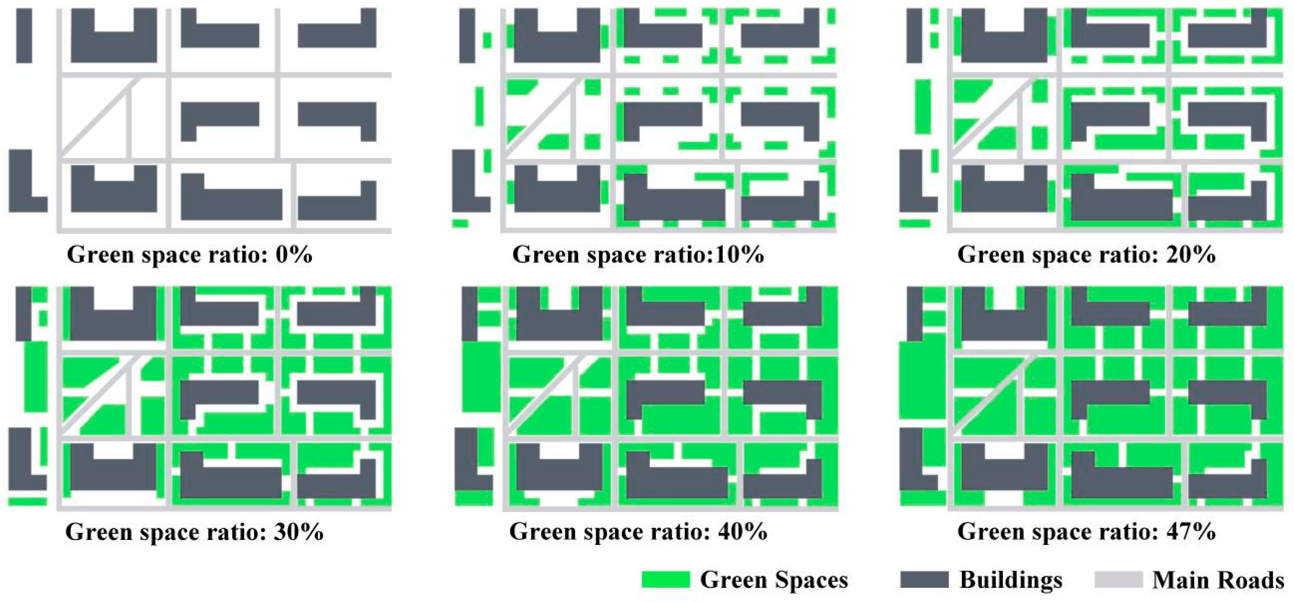
2.5.2. Model Construction: Impact of Green Space Ratios on Bioaerosol Concentrations
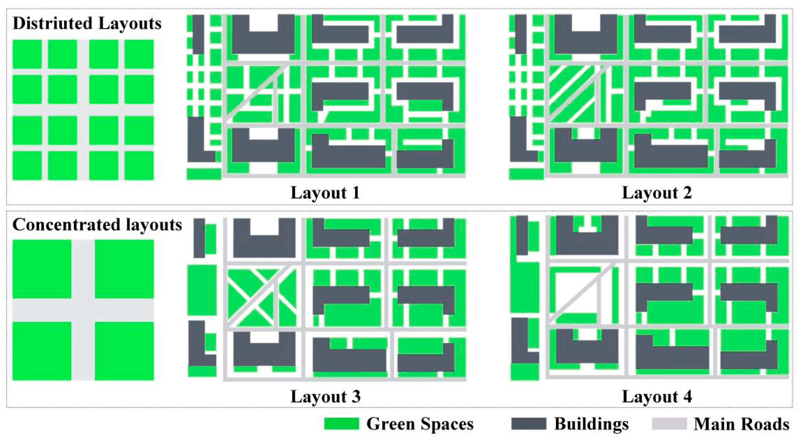
2.5.3. Model Construction: Impact of Green Space Layouts on Bioaerosol Concentrations
Overall Layouts
- Group 1: Distributed and Concentrated Layouts
Local Layouts
- Group 2: Roadside Green Spaces Retreat
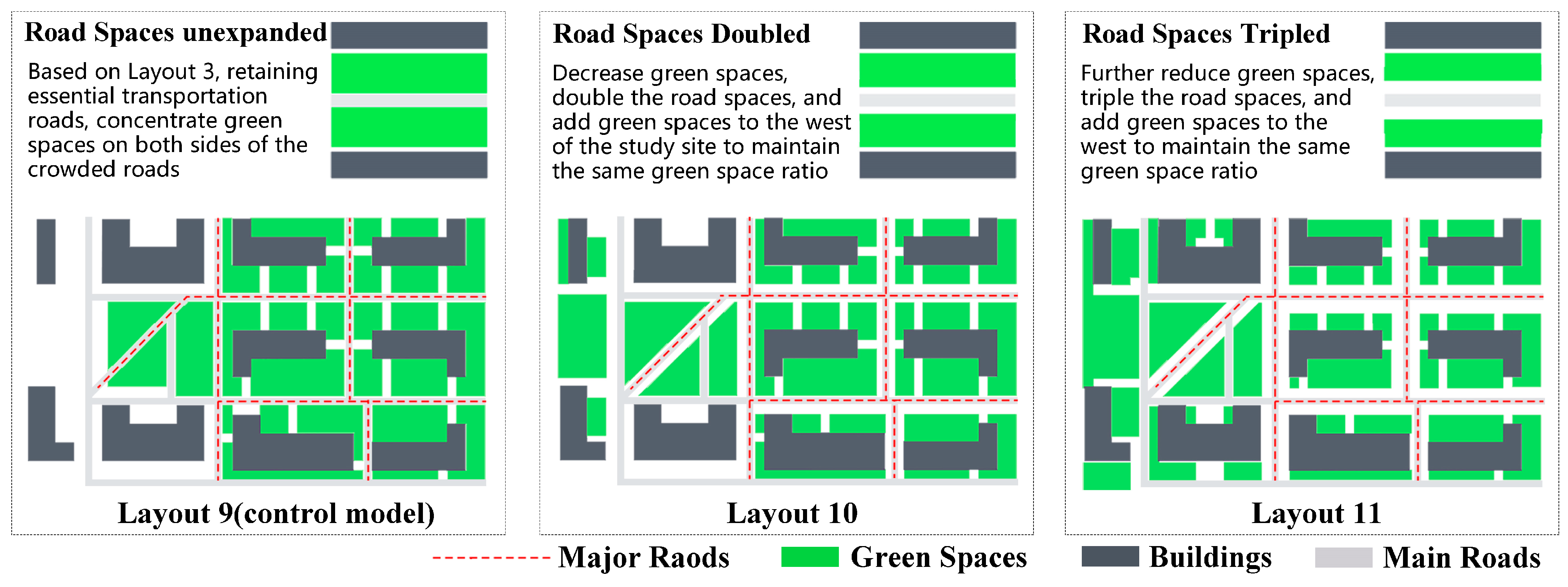
- Group 3: Road Spaces Expansion
- Group 4: Intersection Green Spaces Chamfering
2.6. Data Processing
3. Results
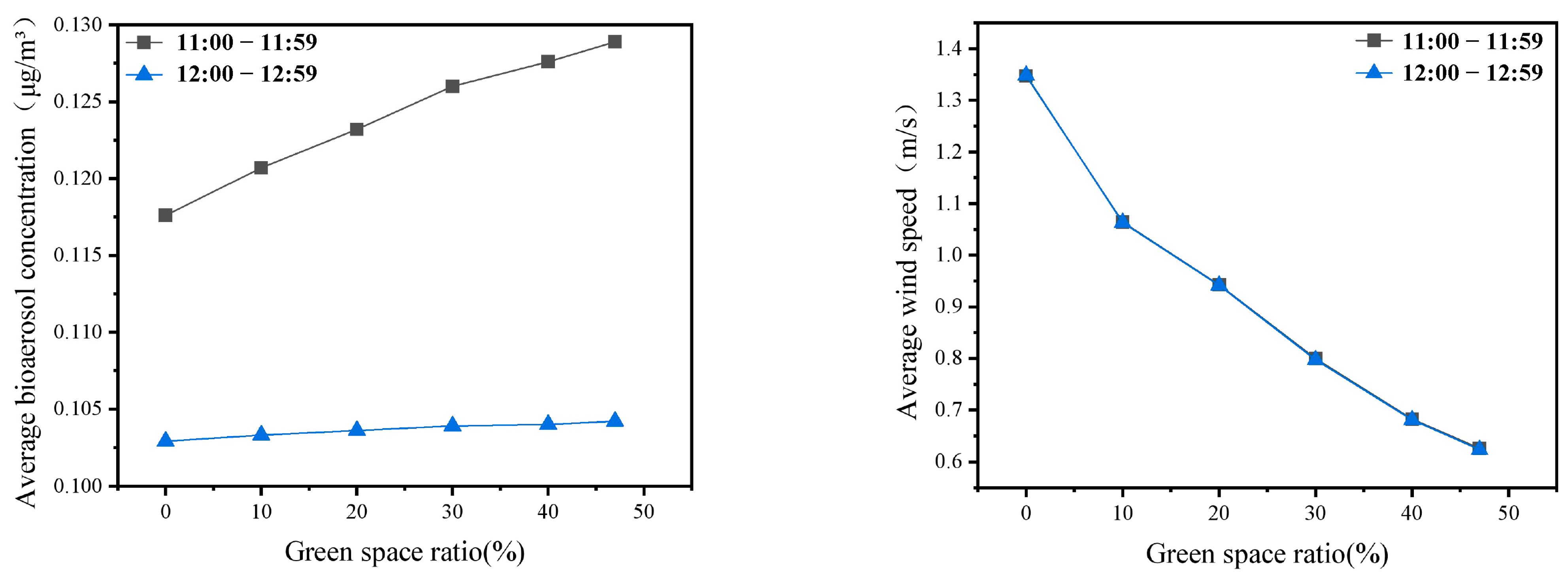
3.1. Impact of Green Space Ratios on Bioaerosol Concentrations
3.2. Impact of Green Space Layouts on Bioaerosol Concentrations
3.2.1. Overall Layouts
- Group 1: Distributed and Concentrated Layouts
3.2.2. Local Layouts
- Group 2: Roadside Green Spaces Retreat
- Group 3: Road Spaces Expansion
- Group 4: Intersection Green Spaces Chamfering
4. Discussion
5. Conclusions
Author Contributions
Funding
Institutional Review Board Statement
Informed Consent Statement
Data Availability Statement
Acknowledgments
Conflicts of Interest
Nomenclature
| r | radius of bioaerosol droplets, 2.5 × 10⁻⁶ m; |
| ρ | density of bioaerosol droplets, 1 × 10¹⁵ μg/m3; |
| m | mass of a single biological bioaerosol droplet, μg; |
| n | the number of bioaerosol droplets produced by a single cough, 1 × 10⁶; |
| k | ratio of bioaerosol droplets produced by breathing to coughing, 1/10; |
| M | mass of bioaerosol produced in a single breath, μg; |
| v | walking speed of an adult, 1.5 m/s; |
| t | duration of a single adult breath, 3 s; |
| l | distance covered by an adult during a single breath, m; |
| V0 | bioaerosol pollution release rate from an adult, µg/m·s·person; |
| N | pedestrian flow on the road, person/min (Table 1); |
| V | release rate of the linear pollution source, µg/m·s; |
References
- Brandl, H. Bioaerosols in Indoor Environment—A Review with Special Reference to Residential and Occupational Locations. Open Environ. Biol. Monit. J. 2011, 4, 83–96. [Google Scholar] [CrossRef]
- Ariya, P.A.; Amyot, M. New Directions: The Role of Bioaerosols in Atmospheric Chemistry and Physics. Atmos. Environ. 2004, 38, 1231–1232. [Google Scholar] [CrossRef]
- Archer, J.; McCarthy, L.P.; Symons, H.E.; Watson, N.A.; Orton, C.M.; Browne, W.J.; Harrison, J.; Moseley, B.; Philip, K.E.J.; Calder, J.D.; et al. Comparing Aerosol Number and Mass Exhalation Rates from Children and Adults during Breathing, Speaking and Singing. Interface Focus 2022, 12, 20210078. [Google Scholar] [CrossRef] [PubMed]
- Yan, J.; Grantham, M.; Pantelic, J.; Bueno De Mesquita, P.J.; Albert, B.; Liu, F.; Ehrman, S.; Milton, D.K.; EMIT Consortium; Adamson, W.; et al. Infectious Virus in Exhaled Breath of Symptomatic Seasonal Influenza Cases from a College Community. Proc. Natl. Acad. Sci. USA 2018, 115, 1081–1086. [Google Scholar] [CrossRef] [PubMed]
- Van Doremalen, N.; Bushmaker, T.; Morris, D.H.; Holbrook, M.G.; Gamble, A.; Williamson, B.N.; Tamin, A.; Harcourt, J.L.; Thornburg, N.J.; Gerber, S.I.; et al. Aerosol and Surface Stability of SARS-CoV-2 as Compared with SARS-CoV-1. N. Engl. J. Med. 2020, 382, 1564–1567. [Google Scholar] [CrossRef] [PubMed]
- Acuto, M. COVID-19: Lessons for an Urban(Izing) World. One Earth 2020, 2, 317–319. [Google Scholar] [CrossRef] [PubMed]
- Bolashikov, Z.D.; Melikov, A.K. Methods for Air Cleaning and Protection of Building Occupants from Airborne Pathogens. Build. Environ. 2009, 44, 1378–1385. [Google Scholar] [CrossRef] [PubMed]
- Zhen, Q.; Fang, Z.G.; Wang, Y.Q.; Ouyang, Z.Y. Bacterial characteristics in atmospheric haze and potential impacts on human health. Acta Ecol. Sin. 2019, 39, 2244–2254. [Google Scholar] [CrossRef]
- Hu, W.X.; Ding, F.; Song, W.H.; Liu, X.H. The Influence of Green Space Disposition Mode on Bacteria Content in Air. J. Environ. Health 2009, 26, 546. [Google Scholar] [CrossRef]
- Rendana, M. Impact of the Wind Conditions on COVID-19 Pandemic: A New Insight for Direction of the Spread of the Virus. Urban Clim. 2020, 34, 100680. [Google Scholar] [CrossRef]
- Coccia, M. How Do Low Wind Speeds and High Levels of Air Pollution Support the Spread of COVID-19? Atmospheric Pollut. Res. 2021, 12, 437–445. [Google Scholar] [CrossRef] [PubMed]
- Meo, S.A.; Almutairi, F.J.; Abukhalaf, A.A.; Usmani, A.M. Effect of Green Space Environment on Air Pollutants PM2.5, PM10, CO, O3, and Incidence and Mortality of SARS-CoV-2 in Highly Green and Less-Green Countries. Int. J. Environ. Res. Public Health 2021, 18, 13151. [Google Scholar] [CrossRef] [PubMed]
- Wu, X.; Nethery, R.C.; Sabath, M.B.; Braun, D.; Dominici, F. Air pollution and COVID-19 mortality in the United States: Strengths and limitations of an ecological regression analysis. Sci. Adv. 2020, 6, eabd4049. [Google Scholar] [CrossRef]
- Bouketta, S.; Bouchahm, Y. Numerical Evaluation of Urban Geometry’s Control of Wind Movements in Outdoor Spaces during Winter Period. Case Mediterr. Climate. Renew. Energy 2020, 146, 1062–1069. [Google Scholar] [CrossRef]
- Leng, J.; Wang, Q.; Liu, K. Sustainable Design of Courtyard Environment: From the Perspectives of Airborne Diseases Control and Human Health. Sustain. Cities Soc. 2020, 62, 102405. [Google Scholar] [CrossRef] [PubMed]
- El Samaty, H.S.; Waseef, A.A.E.; Badawy, N.M. The Effects of City Morphology on Airborne Transmission of COVID-19. Case Study: Port Said City, Egypt. Urban Clim. 2023, 50, 101577. [Google Scholar] [CrossRef] [PubMed]
- Zhang, J.; Yu, Z.; Zhao, B.; Sun, R.; Vejre, H. Links between Green Space and Public Health: A Bibliometric Review of Global Research Trends and Future Prospects from 1901 to 2019. Environ. Res. Lett. 2020, 15, 063001. [Google Scholar] [CrossRef]
- Jabbar, M.; Yusoff, M.M.; Shafie, A. Assessing the Role of Urban Green Spaces for Human Well-Being: A Systematic Review. GeoJournal 2022, 87, 4405–4423. [Google Scholar] [CrossRef] [PubMed]
- Yli-Pelkonen, V.; Setälä, H.; Viippola, V. Urban Forests near Roads Do Not Reduce Gaseous Air Pollutant Concentrations but Have an Impact on Particles Levels. Landsc. Urban Plan. 2017, 158, 39–47. [Google Scholar] [CrossRef]
- Oksanen, E.; Kontunen-Soppela, S. Plants Have Different Strategies to Defend against Air Pollutants. Curr. Opin. Environ. Sci. Health 2021, 19, 100222. [Google Scholar] [CrossRef]
- Lei, Y.; Davies, G.M.; Jin, H.; Tian, G.; Kim, G. Scale-Dependent Effects of Urban Greenspace on Particulate Matter Air Pollution. Urban For. Urban Green. 2021, 61, 127089. [Google Scholar] [CrossRef]
- Diener, A.; Mudu, P. How Can Vegetation Protect Us from Air Pollution? A Critical Review on Green Spaces’ Mitigation Abilities for Air-Borne Particles from a Public Health Perspective—With Implications for Urban Planning. Sci. Total Environ. 2021, 796, 148605. [Google Scholar] [CrossRef] [PubMed]
- Huang, Z.; Wu, C.; Teng, M.; Lin, Y. Impacts of Tree Canopy Cover on Microclimate and Human Thermal Comfort in a Shallow Street Canyon in Wuhan, China. Atmosphere 2020, 11, 588. [Google Scholar] [CrossRef]
- Guo, Y.; Xiao, Q.; Ling, C.; Teng, M.; Wang, P.; Xiao, Z.; Wu, C. The Right Tree for the Right Street Canyons: An Approach of Tree Species Selection for Mitigating Air Pollution. Build. Environ. 2023, 245, 110886. [Google Scholar] [CrossRef]
- Xing, Y.; Brimblecombe, P. Trees and Parks as “the Lungs of Cities”. Urban For. Urban Green. 2020, 48, 126552. [Google Scholar] [CrossRef]
- Corada, K.; Woodward, H.; Alaraj, H.; Collins, C.M.; De Nazelle, A. A Systematic Review of the Leaf Traits Considered to Contribute to Removal of Airborne Particulate Matter Pollution in Urban Areas. Environ. Pollut. 2021, 269, 116104. [Google Scholar] [CrossRef] [PubMed]
- Ortolani, C. The Importance of Local Scale for Assessing, Monitoring and Predicting of Air Quality in Urban Areas. Sustain. Cities Soc. 2016, 26, 150–160. [Google Scholar] [CrossRef]
- Huang, C.-W.; Lin, M.-Y.; Khlystov, A.; Katul, G. The Effects of Leaf Area Density Variation on the Particle Collection Efficiency in the Size Range of Ultrafine Particles (UFP). Environ. Sci. Technol. 2013, 47, 11607–11615. [Google Scholar] [CrossRef]
- Wróblewska, K.; Jeong, B.R. Effectiveness of Plants and Green Infrastructure Utilization in Ambient Particulate Matter Removal. Environ. Sci. Eur. 2021, 33, 110. [Google Scholar] [CrossRef]
- Shi, Y.; Ren, C.; Lau, K.K.-L.; Ng, E. Investigating the Influence of Urban Land Use and Landscape Pattern on PM2.5 Spatial Variation Using Mobile Monitoring and WUDAPT. Landsc. Urban Plan. 2019, 189, 15–26. [Google Scholar] [CrossRef]
- Taleghani, M.; Clark, A.; Swan, W.; Mohegh, A. Air pollution in a microclimate; the impact of different green barriers on the dispersion. Sci. Total Environ. 2020, 711, 134649. [Google Scholar] [CrossRef] [PubMed]
- Dai, F.; Deng, Y.; Chen, M.; Guo, X.H. Effects of Green Space Layout on PM2.5 in Different Types of Residential Areas Based on ENVI-met Simulation. Landsc. Archit. 2021, 28, 70–76. [Google Scholar] [CrossRef]
- Huang, Y.; Lei, C.; Liu, C.-H.; Perez, P.; Forehead, H.; Kong, S.; Zhou, J.L. A Review of Strategies for Mitigating Roadside Air Pollution in Urban Street Canyons. Environ. Pollut. 2021, 280, 116971. [Google Scholar] [CrossRef] [PubMed]
- Jin, X.; Yang, L.; Du, X.; Yang, Y. Transport Characteristics of PM2.5 inside Urban Street Canyons: The Effects of Trees and Vehicles. Build. Simul. 2017, 10, 337–350. [Google Scholar] [CrossRef]
- Xue, F. The Impact of Roadside Trees on Traffic Released PM10 in Urban Street Canyon: Aerodynamic and Deposition Effects. Sustain. Cities Soc. 2017, 30, 195–204. [Google Scholar] [CrossRef]
- Tomson, M.; Kumar, P.; Barwise, Y.; Perez, P.; Forehead, H.; French, K.; Morawska, L.; Watts, J.F. Green Infrastructure for Air Quality Improvement in Street Canyons. Environ. Int. 2021, 146, 106288. [Google Scholar] [CrossRef] [PubMed]
- Jeanjean, A.P.R.; Buccolieri, R.; Eddy, J.; Monks, P.S.; Leigh, R.J. Air quality affected by trees in real street canyons: The case of Marylebone neighbourhood in central London. Urban For. Urban Green. 2017, 22, 41–53. [Google Scholar] [CrossRef]
- Chen, M.; Dai, F.; Yang, B.; Zhu, S. Effects of Urban Green Space Morphological Pattern on Variation of PM2.5 Concentration in the Neighborhoods of Five Chinese Megacities. Build. Environ. 2019, 158, 1–15. [Google Scholar] [CrossRef]
- Li, K.; Li, C.; Liu, M.; Hu, Y.; Wang, H.; Wu, W. Multiscale Analysis of the Effects of Urban Green Infrastructure Landscape Patterns on PM2.5 Concentrations in an Area of Rapid Urbanization. J. Clean. Prod. 2021, 325, 129324. [Google Scholar] [CrossRef]
- Cai, L.; Zhuang, M.; Ren, Y. A landscape scale study in Southeast China investigating the effects of varied green space types on atmospheric PM2.5 in mid-winter. Urban For. Urban Green. 2020, 49, 126607. [Google Scholar] [CrossRef]
- Wu, H.; Yang, C.; Chen, J.; Yang, S.; Lu, T.; Lin, X. Effects of Green Space Landscape Patterns on Particulate Matter in Zhejiang Province, China. Atmos. Pollut. Res. 2018, 9, 923–933. [Google Scholar] [CrossRef]
- Bi, S.; Dai, F.; Chen, M.; Xu, S. A new framework for analysis of the morphological spatial patterns of urban green space to reduce PM2.5 pollution: A case study in Wuhan, China. Sustain. Cities Soc. 2022, 82, 103900. [Google Scholar] [CrossRef]
- Wu, J.; Xie, W.; Li, W.; Li, J. Effects of Urban Landscape Pattern on PM2.5 Pollution—A Beijing Case Study. PLoS ONE 2015, 10, e0142449. [Google Scholar] [CrossRef] [PubMed]
- Zhao, S.; Guo, Q.; Gao, N. Influence of Different Vertical Greening Modes on Bioaerosol Control: A Case Study of Environment Simulation of Liujiaojing Future Community in Linhai City, Zhejiang Province. Landsc. Archit. 2023, 30, 94–101. [Google Scholar] [CrossRef]
- Bruse, M. ENVI-Met Implementation of the Gas/Particle Dispersion and Deposition Model PDDM. Available online: https://www.envi-met.net/documents/sources.PDF (accessed on 12 June 2023).
- Salata, F.; Golasi, I.; De Lieto Vollaro, R.; De Lieto Vollaro, A. Urban microclimate and outdoor thermal comfort. A proper procedure to fit ENVI-met simulation outputs to experimental data. Sustain. Cities Soc. 2016, 26, 318–343. [Google Scholar] [CrossRef]
- Nasrollahi, N.; Hatami, M.; Khastar, S.R.; Taleghani, M. Numerical evaluation of thermal comfort in traditional courtyards to develop new microclimate design in a hot and dry climate. Sustain. Cities Soc. 2017, 35, 449–467. [Google Scholar] [CrossRef]
- Deshmukh, P.; Isakov, V.; Venkatram, A.; Yang, B.; Zhang, K.M.; Logan, R.; Baldauf, R. The effects of roadside vegetation characteristics on local, near-road air quality. Air Qual. Atmos. Health 2019, 12, 259–270. [Google Scholar] [CrossRef] [PubMed]
- Morakinyo, T.E.; Lai, A.; Lau, K.K.-L.; Ng, E. Thermal benefits of vertical greening in a high-density city: Case study of Hong Kong. Urban For. Urban Green. 2019, 37, 42–55. [Google Scholar] [CrossRef]
- Ma, X.; Zhao, J.; Zhang, L.; Wang, M.; Cheng, Z. The Deviation Between the Field Measurement and ENVI-Met Outputs in Winter- A Cases Study in a Traditional Dwelling Settlement of Northern China. Envrion. Model Assess. 2023, 28, 817–830. [Google Scholar] [CrossRef]
- Gu, K.; Qian, Z.; Fang, Y.H.; Sun, Z.; Wen, H. Influence of vegetation arrangement on PM2.5 in urban roadside based on ENVImet. Acta Ecol. Sin. 2020, 40, 4340–4350. [Google Scholar]
- Liu, J.; Guo, H.; Zhang, L.; Lu, L. Impact of Urbanization on Vegetation Phenology: A Study in the Beijing-Tianjin-Tangshan Region. Remote Sens. Technol. Appl. 2014, 29, 286–292. [Google Scholar]
- Cox, C.S. Physical Aspects of Bioaerosol Particles. In Bioaerosols Handbook; Taylor & Francis: Oxfordshire, UK, 1955; pp. 15–25. [Google Scholar] [CrossRef]
- Papineni, R.S.; Rosenthal, F.S. The Size Distribution of Droplets in the Exhaled Breath of Healthy Human Subjects. J. Aerosol Med. 1997, 10, 105–116. [Google Scholar] [CrossRef] [PubMed]
- Xie, X.; Li, Y.; Chwang, A.T.Y.; Ho, P.L.; Seto, W.H. How Far Droplets Can Move in Indoor Environments ? Revisiting the Wells Evaporation?Falling Curve. Indoor Air 2007, 17, 211–225. [Google Scholar] [CrossRef] [PubMed]
- Kong, F.; Nakagoshi, N. Spatial-Temporal Gradient Analysis of Urban Green Spaces in Jinan, China. Landsc. Urban Plan. 2006, 78, 147–164. [Google Scholar] [CrossRef]
- Yu, Z.; Yang, G.; Zuo, S.; Jørgensen, G.; Koga, M.; Vejre, H. Critical Review on the Cooling Effect of Urban Blue-Green Space: A Threshold-Size Perspective. Urban For. Urban Green. 2020, 49, 126630. [Google Scholar] [CrossRef]
- Ferrini, F.; Fini, A.; Mori, J.; Gori, A. Role of Vegetation as a Mitigating Factor in the Urban Context. Sustainability 2020, 12, 4247. [Google Scholar] [CrossRef]
- Nieuwenhuijsen, M.J. New Urban Models for More Sustainable, Liveable and Healthier Cities Post Covid19; Reducing Air Pollution, Noise and Heat Island Effects and Increasing Green Space and Physical Activity. Environ. Int. 2021, 157, 106850. [Google Scholar] [CrossRef] [PubMed]
- Elmqvist, T.; Setälä, H.; Handel, S.; Van Der Ploeg, S.; Aronson, J.; Blignaut, J.; Gómez-Baggethun, E.; Nowak, D.; Kronenberg, J.; De Groot, R. Benefits of Restoring Ecosystem Services in Urban Areas. Curr. Opin. Environ. Sustain. 2015, 14, 101–108. [Google Scholar] [CrossRef]
- Tian, F.; Yu, Z.; Cai, M. Numerical Simulation of Gaseous Pollutants Dispersion at Street-Canyon Road Intersection. Res. Environ. Sci. 2008, 2, 2180–2183. [Google Scholar] [CrossRef]


| Road Numbers | Road Pedestrian Flow (People/min) 11:00–11:59 AM | Road Pedestrian Flow (People/min) 12:00–12:59 AM | ||||||||||
|---|---|---|---|---|---|---|---|---|---|---|---|---|
| 5.5 | 5.8 | 5.9 | 5.10 | 5.11 | 5-Day Average | 5.5 | 5.8 | 5.9 | 5.10 | 5.11 | 5-Day Average | |
| 1 | 14 | 17 | 17 | 12 | 13 | 15 | 13 | 9 | 6 | 13 | 16 | 11 |
| 2 | 6 | 11 | 22 | 9 | 7 | 11 | 10 | 9 | 10 | 11 | 12 | 10 |
| 3 | 13 | 10 | 9 | 9 | 13 | 11 | 12 | 9 | 10 | 14 | 10 | 11 |
| 4 | 2 | 1 | 2 | 1 | 2 | 2 | 1 | 2 | 1 | 4 | 2 | 2 |
| 5 | 3 | 3 | 3 | 3 | 4 | 3 | 3 | 3 | 6 | 3 | 2 | 3 |
| 6 | 16 | 34 | 24 | 21 | 29 | 25 | 22 | 17 | 25 | 21 | 16 | 20 |
| 7 | 12 | 7 | 10 | 8 | 10 | 9 | 10 | 7 | 4 | 7 | 12 | 8 |
| 8 | 13 | 16 | 17 | 13 | 19 | 16 | 8 | 11 | 17 | 14 | 16 | 13 |
| 9 | 9 | 16 | 13 | 12 | 20 | 14 | 11 | 10 | 14 | 11 | 13 | 12 |
| 10 | 11 | 13 | 15 | 11 | 14 | 13 | 8 | 9 | 11 | 10 | 14 | 10 |
| 11 | 9 | 8 | 10 | 6 | 5 | 8 | 9 | 5 | 5 | 4 | 8 | 6 |
| 12 | 14 | 9 | 12 | 9 | 13 | 11 | 10 | 9 | 12 | 12 | 9 | 10 |
| 13 | 6 | 6 | 9 | 5 | 4 | 6 | 5 | 5 | 7 | 4 | 10 | 6 |
| 14 | 3 | 2 | 1 | 3 | 4 | 3 | 0 | 1 | 1 | 2 | 2 | 1 |
| Road Numbers | Bioaerosol Release Rate for Linear Pollutant Source, 11:00–11:59 AM (μg/m·s) | Bioaerosol Release Rate for Linear Pollutant Source, 12:00–12:59 AM (μg/m·s) |
|---|---|---|
| 1 | 0.118 | 0.092 |
| 2 | 0.089 | 0.084 |
| 3 | 0.087 | 0.089 |
| 4 | 0.013 | 0.016 |
| 5 | 0.026 | 0.027 |
| 6 | 0.200 | 0.163 |
| 7 | 0.076 | 0.065 |
| 8 | 0.126 | 0.107 |
| 9 | 0.113 | 0.095 |
| 10 | 0.103 | 0.084 |
| 11 | 0.061 | 0.050 |
| 12 | 0.092 | 0.084 |
| 13 | 0.049 | 0.050 |
| 14 | 0.021 | 0.010 |
| Parameter Category | Parameter Name | Input Value |
|---|---|---|
| Geographic location | Latitude and longitude | Beijing, China (39.96° N, 116.30° E) |
| Time zone | Time zone | China Standard Time/GMT + 8 |
| Simulation time | Start time | 10 May 2023, 11:00 AM |
| End time | 10 May 2023, 1:00 PM | |
| Duration | 2 h | |
| Meteorological conditions (Sourse: The real-time data from http://hz.hjhj-e.com/, accessed on 15 May 2023) | Wind direction (0:N, 90:E, 180:S, 270:W) | 135 |
| Wind speed | 2 m/s | |
| Initial temperature | 24 °C | |
| Relative humidity | 24% | |
| Plant parameters | Grass | 25 mm height, 2D grass |
| Trees | 10 m height, 2D trees | |
| Pollution source settings | Pollution source type | Linear (line) |
| Pollution source category | Particle | |
| Background pollution concentration | 0.1 μg/m3 | |
| Linear pollutant source release rate | Refer to Table 2 |
| Layouts | Number of Patches (NP) | Landscape Split Index (LSI) |
|---|---|---|
| Layout 1 | 60 | 42.0525 |
| Layout 2 | 70 | 44.7683 |
| Layout 3 | 38 | 25.1016 |
| Layout 4 | 39 | 23.9367 |
| 11:00–11:59 AM Average Bioaerosol Concentration | 12:00–12:59 AM Average Bioaerosol Concentration | |
|---|---|---|
| Green space ratio | 0.994 ** | 0.986 ** |
| 11:00–11:59 AM Average wind speed | −0.993 ** | |
| 12:00–12:59 AM Average wind speed | −0.997 ** |
| Green Space Ratio (%) | 11:00–11:59 AM Average Bioaerosol Concentration (μg/m3) | 11:00−11:59 AM Average Wind Speed (m/s) | 12:00−12:59 AM Average Bioaerosol Concentration (μg/m3) | 12:00–12:59 AM Average Wind Speed (m/s) |
|---|---|---|---|---|
| 0 | 0.1176 | 1.3474 | 0.1029 | 1.3487 |
| 10 | 0.1207 | 1.0641 | 0.1033 | 1.0632 |
| 20 | 0.1232 | 0.9425 | 0.1036 | 0.9416 |
| 30 | 0.1260 | 0.7997 | 0.1039 | 0.7973 |
| 40 | 0.1276 | 0.6824 | 0.1040 | 0.6809 |
| 47 | 0.1289 | 0.6260 | 0.1042 | 0.6234 |
| Simulation Plan Number | Average Bioaerosol Concentration (μg/m³) | Average Wind Speed (m/s) |
|---|---|---|
| Layout 1 | 0.1271 | 0.7062 |
| Layout 2 | 0.1272 | 0.6946 |
| Layout 3 | 0.1256 | 0.8145 |
| Layout 4 | 0.1256 | 0.8228 |
| Simulation Plan Number | Average Bioaerosol Concentration (μg/m3) | Average Wind Speed (m/s) |
|---|---|---|
| Layout 9 | 0.1273 | 0.8283 |
| Layout 10 | 0.1261 | 0.8391 |
| Layout 11 | 0.1243 | 0.8314 |
Disclaimer/Publisher’s Note: The statements, opinions and data contained in all publications are solely those of the individual author(s) and contributor(s) and not of MDPI and/or the editor(s). MDPI and/or the editor(s) disclaim responsibility for any injury to people or property resulting from any ideas, methods, instructions or products referred to in the content. |
© 2024 by the authors. Licensee MDPI, Basel, Switzerland. This article is an open access article distributed under the terms and conditions of the Creative Commons Attribution (CC BY) license (https://creativecommons.org/licenses/by/4.0/).
Share and Cite
Jian, W.; He, H.; Wang, B.; Liu, Z. Investigating the Impact of Green Space Ratio and Layout on Bioaerosol Concentrations in Urban High-Density Areas: A Simulation Study in Beijing, China. Sustainability 2024, 16, 3688. https://doi.org/10.3390/su16093688
Jian W, He H, Wang B, Liu Z. Investigating the Impact of Green Space Ratio and Layout on Bioaerosol Concentrations in Urban High-Density Areas: A Simulation Study in Beijing, China. Sustainability. 2024; 16(9):3688. https://doi.org/10.3390/su16093688
Chicago/Turabian StyleJian, Wenchen, Hao He, Boya Wang, and Zhicheng Liu. 2024. "Investigating the Impact of Green Space Ratio and Layout on Bioaerosol Concentrations in Urban High-Density Areas: A Simulation Study in Beijing, China" Sustainability 16, no. 9: 3688. https://doi.org/10.3390/su16093688
APA StyleJian, W., He, H., Wang, B., & Liu, Z. (2024). Investigating the Impact of Green Space Ratio and Layout on Bioaerosol Concentrations in Urban High-Density Areas: A Simulation Study in Beijing, China. Sustainability, 16(9), 3688. https://doi.org/10.3390/su16093688