Enhancing Traffic Sustainability: An Analysis of Isolation Intersection Effectiveness through Fixed Time and Logic Control Design Using VisVAP Algorithm

Abstract

This paper addresses the limitations of the fixed-time approach in traffic signal control, which can lead to bottlenecks and inefficiencies. Proposing an alternative algorithm based on design logic control, the study integrates data from inductive detectors and non-linear traffic flow rates to optimize signaling plans. Analytical models are developed for both fixed and semi-actuated traffic signal control approaches, with PTV Vissim software (version 8, 64 bit) used for simulation. The design logic control dynamically adjusts signaling plans, determining the duration of the green interval for the secondary road based on arrival traffic flow. In the absence of traffic, it eliminates the green interval, advancing to the next phase, thereby reducing cycle time. This dynamic adjustment follows a conditional “if-then” statement, optimizing traffic signal operation. The design logic control algorithm was tested in a real isolation intersection with four scenarios, using non-linear traffic flow rate data for one peak hour. Results demonstrated that the proposed design logic control, based on the Semi-Actuated Traffic Signal Control (SATSC) approach, outperformed the commonly used Fixed-Time Signal Control (FTSC) with overall reduction of queue lengths by 39.6% and reduction of vehicle delays by 51.3%. The findings suggest its viability as a solution for many cities, contributing to a more sustainable traffic system.

1. Introduction

In an era of rapid urbanization, the challenges of urban traffic become increasingly complex, directly impacting the quality of life in modern cities. This is accompanied by a rise in motorization levels, leading to time loss, increased fuel consumption, and various environmental problems [1]. Traffic congestion in urban areas has emerged as a significant issue globally, prompting researchers to consistently explore systems that can mitigate this phenomenon and enhance permeability within existing road networks. Additionally, the absence of effective traffic management significantly contributes to this situation [2]. The efficiency of traffic regulation at road intersections through traffic signal control (TSC) depends on the ability to balance the flow of vehicles without worsening queue lengths, delays, and density [3]. Despite these challenges, TSC play a crucial role in providing effective solutions to the complexities of road traffic, ensuring optimal control within the network, while simultaneously informing drivers as active participants in road traffic [4]. However, due to the poorly synchronized timing of the signalization plan, TSCs often create obstacles to the normal flow of traffic on the road network. Prior to exploring the various operational modalities of TSC, it is crucial to acknowledge that the majority of intersections adopt efficient and well-managed signal control strategies [5].

These strategies include Fixed-Time Signal Control (FTSC), Actuated Time Signal Control (ATSC), or a combination of both, along with Semi Actuated Traffic Signal Control (SATSC) and Adaptive Traffic Signal Control (ADTSC). Understanding these operational modes is crucial for comprehending the nuanced dynamics of traffic signalization and its impact on intersection efficiency. In FTSC, control is based on specific signal durations, while in ATSC, control utilizes predetermined reductions and extensions to adjust phases based on vehicle detection. On the other hand, ADTSC is characterized by its continuous sensitivity to traffic conditions, adjusting signal timing in accordance with the prevailing circumstances [6].

Due to the non-linearity of traffic flow during different time periods at signalized intersections, unfortunately, it is difficult to define optimal values for the phases or extensions for green intervals in long-term periods [7]. The predefined nature of signalization plans further limits the adaptability of these strategies to varying traffic demands throughout the day, particularly during unexpected events [8]. As a result, such strategies tend to cause long queues and excessive delays due to overestimated or underestimated timing. The optimization of signal performance at signalized intersections stands as a paramount concern for traffic engineers in urban areas. The goal is to enhance performance indicators and promote sustainable transport efficiency for all users without requiring infrastructure interventions. To address these challenges, this paper [9] proposes a design control logic as an alternative approach, focusing on the inherent nature of the issues rather than treating them solely as optimization problems.

The selection of the design control logic as a new TSC strategy is motivated by the desire to improve flexibility, adaptability, and efficiency in traffic flow management. In this study, a specific investigation was conducted by implementing design logic control to assess the impact of the SATSC strategy at signalized intersections, extending the FTSC strategy. The analysis and comparison of the results aimed at identifying improvements in the current situation and presenting an optimal solution. The design logic control operates by utilizing the arrival flow rate as input to determine the appropriate cycle duration. In this scenario, the cycle is calculated by proportionally splitting the effective green time based on the Semi Actuated Traffic Signal Control (SATSC) strategy [10]. According to this strategy, the design logic control can effectively adjust the signal plan to clear queues formed during red intervals at the traffic light, thereby improving the operational performance of the intersection. This improvement manifests through reductions in delays, queue length, and density. The proposed design logic control is algorithm-based, relying on the minimum and maximum values of the expected arrival traffic flow from the secondary road, as well as the cycle duration determined by the programming logic in the Vehicle Actuated Program (VAP) language (PTV Vissim version 8, 64 bit). Furthermore, the proposed algorithm is grounded in sequential logic, employing if-then statements.

The performance of the designed logic control was assessed using a microsimulation model within the PTV Vissim software, focusing on a specific real-world intersection—namely, the intersection of ‘Mother Theresa’ and ‘Hajrulla Zymi’ roads, which was also a subject of treatment in the Sustainable Mobility Plan of FusheKosovo [11]. Four scenarios were constructed based on field-collected data for a ‘peak hour’. By implementing the simulation according to this algorithm as a test, necessary comparisons were made concerning queue length and delay indicators, as compared to the FTSC strategy. The simulation results indicate that the SATSC with design logic control proves significantly more effective than the FTSC approach, especially when accompanied by interventions in the hardware infrastructure of the signaling system at the intersection.

The structure of the paper is organized into the following chapters. Section 2 provides a literature review. Section 3 presents a detailed overview of the methodology for constructing models related to Traffic Control Signals. In Section 4, a simulation model for the FTSC and SATSC strategies is presented using a specific example as a case study. Section 5 contains the results and necessary evaluations. Finally, Section 6 presents concluding remarks.

2. Related Works

Many authors in their studies have emphasized the need for addressing this topic and have developed various traditional or contemporary design logic control approaches to find the most satisfactory solutions.

Authors in papers [12,13] have been engaged in the application and optimization of TSC using FTSC strategy. However, due to the dynamic nature of traffic, these may not be suitable, because fixed signal plans cannot accommodate every traffic condition. Another approach is ATSC strategy, where the phases of the signaling plan are activated upon the detection of vehicles by detectors on the road [14]. So, for the enhancement of positive effects on intersection performance, strategies such as ATSC have begun to be implemented, due to the advantages it brings in comparison to FTSC [15]. The main effect related the fact that the operation according to ATSC is associated with the ability to update parameters in response to the arrivals of vehicles at the intersection entrance. This is achieved by adjusting the parameters of ATSC strategy, such as the minimum green time interval (MinGT), maximum green time interval (MaxGT), and cycle length. The subsequent section offers an overview of studies conducted in this field.

The application of ATSC strategy is typically found in isolated intersections where TSC operates independently [16]. Akcelik, in his study, proposed a method to assess the average green interval and cycle length with ATSC strategy, respectively aiming to optimize the cycle length based on predicted vehicle arrival headways [17]. Kim and Courage, in their work, proposed a method for designing the maximum green interval with ATSC strategy, aiming to minimize delays for vehicles moving through the intersection [18]. Wu et al., defined the maximum green interval in relation to the movement of the maximum number of left-turning vehicles, where the predetermined number was set at 10 vehicles per lane [19]. In the papers mentioned above, signal control parameters were defined solely in a static manner, based on the expertise of professionals and engineers, along with statistical analyses considering historical data related to vehicular traffic flow at intersection. Moreover, alongside static signal control, dynamic signal control methods for adjusting the duration of the green interval were also explored in response to non-linearity in traffic flow [20]. Therefore, Zhang and Wang, based on data from queue lengths obtained from point detectors, developed a method for dynamically controlling the green interval, including both minimum (MinGT) and maximum (MaxGT) values [21]. Based on the recommendations of HCM 2010 regarding the determination of the typical green time interval and signals provided by static detectors on the road for measurement queue length, Shirvani, Shiri, and Maleki proposed a “fuzzy logic control” approach that dynamically determines the green interval as (MaxGT) [22]. As mentioned earlier, in addition to determining the green interval, another crucial factor in phase timing is the cycle duration. Among the pioneers and well-known figures addressing this issue was Webster, who, as early as 1958, developed the TRRL model with the objective of controlling and minimizing overall delays at intersections [23]. Furthermore, Akcelik extended his research to encompass the number of stops at intersections, providing a more comprehensive exploration of the subject [24].

Additionally, HCM [25] presents a model for calculating cycle duration based on intersection critical demand and measures capacity utilization using the Peak Hour Factor (PHF) in relation to traffic flow over saturation (i.e., v/c ratio, where based on anticipated congestion, the cycle duration can be applied according to various traffic conditions [25].

Swaminathan et al., developed a model related to ATSC for a road segment [26]. As a result of the analysis, it was observed that the average delays reduced by 28% compared to the existing condition through FTSC strategy. Wang et al., addressed the challenge of extending the green time in ATSC strategy, and their results revealed that the optimal values of critical headways, a significant parameter for green interval extension, decreased as traffic demand increased [27]. In comparison to ATSC strategy, which utilize detectors from all branches, specifically the lanes at the intersection’s entrance, to control signal groups, and FTSC strategy that do not use detectors at all, it is possible to combine these two approaches, creating systems referred to as SATSC strategy [28]. In these systems, detectors are only used on secondary roads without the need for detectors on the main road. An advantage of these systems is that they can be effectively applied in coordinated signal control systems. Furthermore, when compared to FTSC strategy, delays on the main road are reduced during low traffic flow conditions [29].

In their paper, Yaru Guo and Jihui Ma proposed a model related to the improvement of the ATSC strategy to enhance the efficiency of intersection movement [30]. For the construction of the model, PTV Vissim software was used to simulate the operational state of different time intervals under the FTSC and ATSC strategies, and improved ATSC strategy based on the actual traffic flow, signal timing, and other intersection data. The simulation results indicated that travel times and delays were reduced with the application of the Adaptive Traffic Signal Control in all considered time periods, as reported in the study [31]. In his study, Dabiri et al. [32], proposes a cost-effective approach to reduce delays in semi-actuated coordinated signal operation without incurring additional costs for installing new detectors or developing adaptive controller systems.

Based on the reviewed studies, it can be observed that optimizing the duration of the green phase, considering parameters such as (MinGT) and (MaxGT) for the optimal choice of the cycle duration, has demonstrated numerous benefits in terms of efficiency and enhancing intersection performance. However, in addition to these considerations, the complete elimination of a phase and its transfer to the subsequent phase in the absence of traffic flow during specific intervals in a certain direction, particularly from the secondary road, according to the repeating cyclical method, remains an issue that has not been adequately addressed. So, for this reason, in this study, both parameters were considered: the selection of optimal parameters for the green interval and the elimination/transfer of the green phase in the absence of traffic flows from the secondary road. This is based on developing an algorithm according to design logic control. This algorithm facilitates the numerical calculation and simulation of optimal parameters under various conditions. The process allows for a comparison of results obtained through simulations and validates the analytical analysis.

3. Material and Methodology

3.1. Overview of the Methodology

In this paper, the concept for measuring the performance parameters of the intersection has been developed by applying the FTSC and SATSC approaches. This concept is composed of three fundamental components that are interconnected among themselves: input parameters, the analytical model, and the simulation model, as presented in Figure 1. In Component 1 of the framework, various elements such as intersection geometry, traffic volume, traffic lights, and detectors are included. This component primarily addresses the physical aspects of the intersection, encompassing factors like layout, traffic volume, configuration of traffic lights, and the use of detectors to monitor traffic conditions.

Analytical models have been developed to calculate signaling plan elements under the FTSC and SATSC strategies. These models offer a systematic and mathematical representation, considering factors like traffic conditions, timings, and relevant parameters. Their purpose is to optimize signaling plans for improved intersection performance under both FTSC and SATSC approaches. The FTSC model utilizes parameters such as signal plan, intervals, critical traffic, lost times, cycle time, and green time. In the SATSC model, three additional parameters—minimum green time, unit extension, and maximal green time—are typically considered, in addition to those used in the FTSC model.

The optimization of the signal plan involves defining performance indicators derived from the simulation model to serve as objectives for signal control. These objectives may encompass minimizing delays or queue length and maximizing throughput. After performing calculations according to analytical models, these parameters were used as inputs for the simulation models built in PTV Vissim software. In both simulation models, FTSC and SATSC, in addition to general parameters like lanes and connectors, vehicle compositions, vehicle inputs, routings, area conflicts, and desired speed, additional modules within the PTV Vissim software framework were applied.

Thus, for the design of signaling plans in the FTSC model, the additional module “Vissig” has been applied, while for the SATSC model, the additional module “VisVAP” has been applied with *.vap and *.pua files. The simulation model is linked to signal control, and movements through the intersection occur according to signal indications.

The signal control component implements the control logic for the intersection and the parameters associated with this logic [33].

The data recording is done by the detector, which is activated by vehicles upon their arrival. The information regarding activation is transmitted to the control logic unit. Vehicles progress in this manner, moving from detector to the stop line, continuing their movement. The detector continuously monitors the queue length in the side lane at each time interval. If the presence of minimal and maximal vehicles in the queue between the stop line and the upstream detector is detected at any time interval, the detector is activated for that specific interval.

Throughout the effective green time, vehicles are discharged from the queue at the saturation flow rate in a deterministic manner. As a result, the optimization module can set parameter values for the simulation model, run the model, and extract performance values from the simulation results. This iterative process continues until an optimal solution is identified. In the following, detailed explanations are provided for the components related to control methods, calculations, and simulations for TSC in one specific case study.

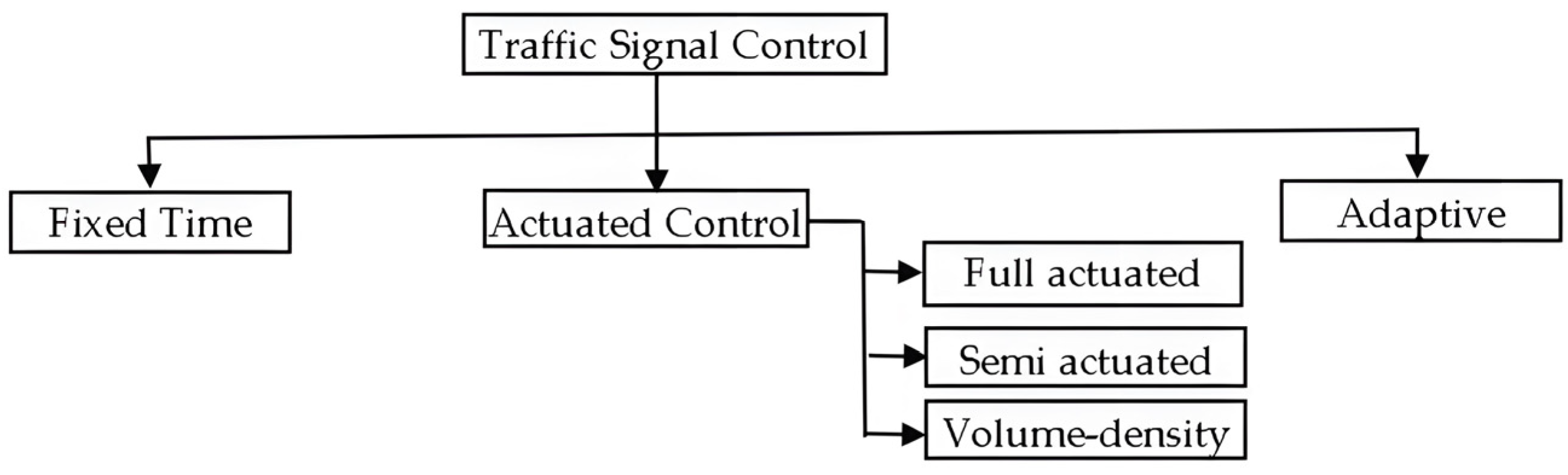
3.2. Methods of Traffic Signal Controls

Traffic Signal Control (TSC) can operate according to basic and intelligent control [34]. The basic control is applied through FTSC, and ATSC strategies includes the control of FATSC (Full Actuated Traffic Signal Control), SATSC (Semi Actuated Traffic Signal Control), and Adaptive Traffic Signal Control (ADTSC). These signal controls respond to traffic demands based on data collected from detectors. Various detection technologies, such as loop detectors and video systems, are utilized to enhance vehicle presence detection capabilities [33]. Inductive loop detectors are more common and widely used in traffic control systems [35]. The basic operating types of TSC are illustrated in Figure 2 [6].

The FTSC mode operates on fixed phases and a predetermined cycle duration, while other modes have dynamic cycle parameters that adjust to traffic demands. FATSC is effective when traffic loads are approximately equal on all roads, while SATSC performs better with less traffic on secondary roads. ADTSC uses detector data for optimal coordination plans. Focusing on FTSC and SATSC for analysis, the choice is influenced by the current FTSC operation at the intersection, facilitating necessary comparisons of performance indicators with SATSC approach.

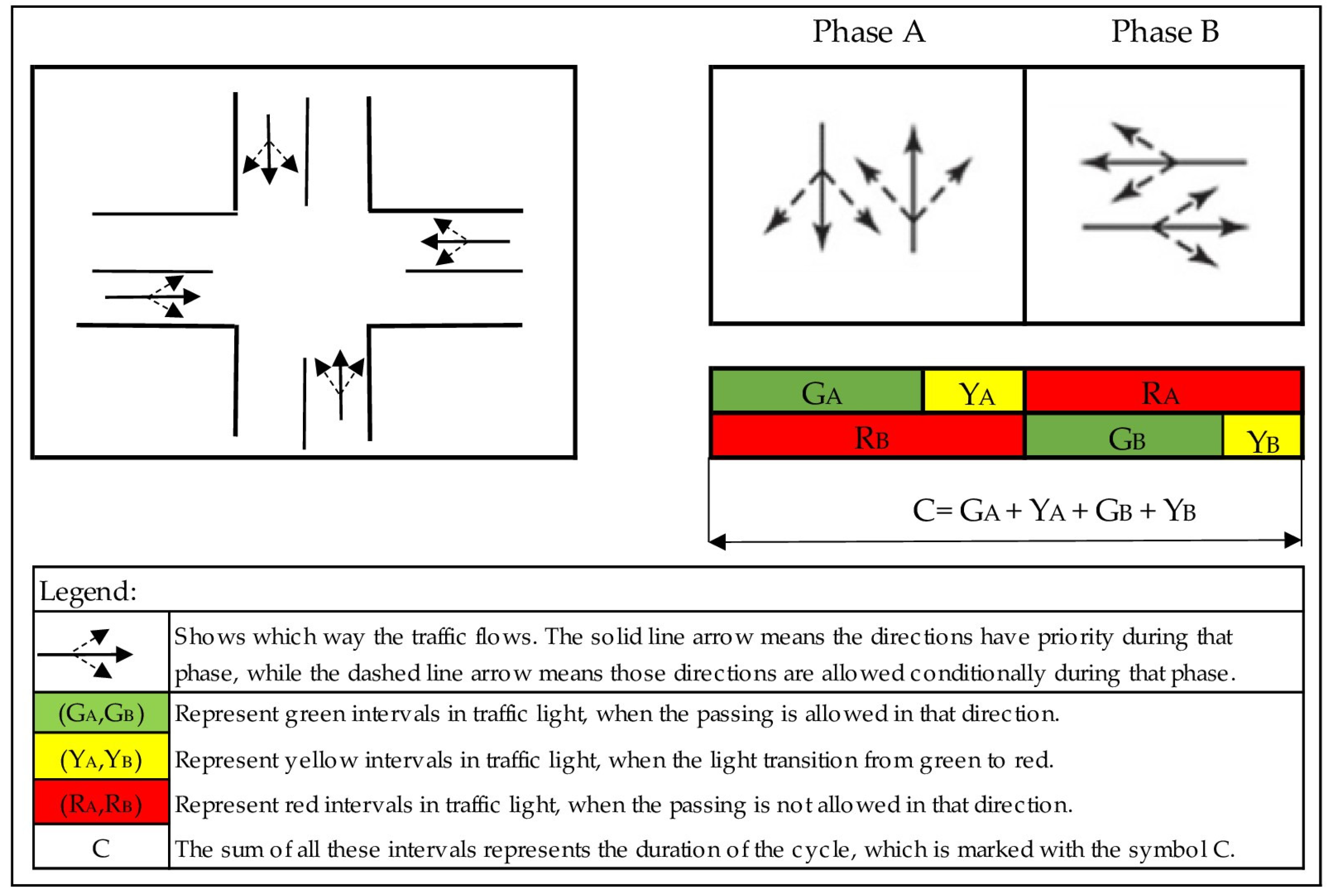
3.2.1. Fixed Time Traffic Signal Control (FTSC)

FTSC strategy, involves managing intersections according to a specific plan for the execution of phases, i.e., signaling plans, over time. The duration and structure of the signaling plan are calculated based on traffic count data. FTSC consists of a series of intervals with fixed durations and repeat the cycle consistently [36]. This type of control does not provide the ability to react to current traffic conditions, but it is possible to configure traffic signal devices to support multiple signaling plans [6]. This enables the adjustment of the signaling plan selection based on the time of day, which is calculated according to the number and categorization of vehicles. There is also the possibility of synchronizing traffic signal devices at multiple intersections using coordinated timing to initiate the service of the same traffic flow simultaneously. This achieves the effect of continuous passage through several intersections, known as the green wave, which forms the basis of arterial corridor management [37]. The positive aspects of FTSC compared to other strategies are: (a) technically relatively simple and cost-effective implementation and, (b) traffic signal devices do not need to be connected to other intersections or a traffic center. The post-implementation cost refers to periodic maintenance and traffic re-surveying to refresh the signal plans [38].

Due to the lack of the ability to react to the current traffic situation, this type of control is not suitable for intersections where there is high and variable traffic demand, also occasional events such as traffic accidents, special events, road works, etc. [39]. Unfortunately, FTSC cannot compensate for unplanned non-linearity in traffic flows and may be inefficient in isolated intersections where traffic arrivals from different approaches are unpredictable [36]. There are some controllers that allow the establishment of different signal cycles at different intervals throughout the day. Older electro-mechanical type traffic signal controllers have the capability to set at least three signaling plans for the periods of maximum morning, afternoon traffic, and a plan for other non-peak periods. Modern controllers allow the implementation of up to 20 different pre-timed signal plans [40]. Indeed, the parameters of traffic signals determine how an intersection can be controlled in relation to the progression of traffic flow. Depending on the configuration of parameters, the intersection can operate under various traffic conditions. The signal control program is determined by the following parameters [41]:

1. Effective phase plan and sequence. The most critical aspect of signal and timing design is the development of an appropriate phase plan. A phase consists of the green interval, plus the change and clearance intervals that follow it. This represents a set of intervals within which movements are respectively allowed or prohibited for a group of vehicles and pedestrians participating in the intersection. In FTSC, all interval durations remain constant during each signal cycle. Thus, the sequence of phases, all green times, and the cycle length are fixed for the time period during which the timing plan is implemented. Yellow and all-red intervals are fixed in FTSC, but in actuated controllers, they can be adjusted, because the situation changes, and these parameters change and are dependent on the traffic demand as detected by detectors at the intersection [42]. The signal phase plans are generally illustrated using phase diagrams and ring diagrams, as graphically presented in Figure 3. A phase diagram illustrates all movements being made in a given phase within a single block of the diagram. A ring diagram illustrates which movements are controlled by each “ring” on a signal controller [43].

2. Interval. An interval is a period of time during which there are no changes in the signal lights. It is the smallest unit of time described within a cycle. There are several types of intervals within the cycle, such as: Green Interval, Change Interval, Amber Interval, Red Interval and Clearance Interval as presented in Figure 4. Two of the most crucial intervals are: the Clearance Interval and the Green Interval [44].

Clearance Interval. The clearance interval consists of the yellow interval ($y$) and all-red intervals $\left(ar\right)$. Intervals of yellow and all-red ensure a safe transition from green to red. The yellow interval is calculated using Equation (1).

$$y=t+\left(\frac{1.47·S_{85}}{2a+64.4·0.01g}\right)$$

(1)

where $y$—duration of the yellow interval (s); $S_{85}$—85th percentile of speed (m/s); $t$—driver’s reaction time (s); $a$—deceleration rate (m/s²); $g$—road grade (%).

The clearance interval is also part of the transition from the “green” to the “red” for a specific group of movements. During the clearance interval, all movements have the red light on the traffic signal. This is the time utilized to allow the passage of vehicles that have just crossed the intersection before releasing other vehicles that are in conflict with them. The clearance interval is denoted by the symbol “$ar$” meaning “all-red” for movement’s “i”. The all-red intervals are a period during which all signals display a red indication. The determination of the duration of clearance interval is done through Equation (2) [28].

$$ar=\frac{w+l}{1.47\ast S_{15}}$$

(2)

where $ar$—duration of the all-red interval (s); $S_{15}$—15th percentile approach speed (m/s); $w$—width of the traversed road (m); $l$—length of the vehicle (m); 1.47 is the converting factor for distance.

The all-red interval is that part of the traffic signal cycle where all entry lanes to the intersection have a red signal. Many cities and countries around the world do not use the all-red interval in their signal plans [45]. Therefore, by using the sequence red (R), Green (G), Amber (A), in this paper, we have added the values of this all-red time interval to the yellow interval, implying that vehicles clear the intersection during the yellow interval.

3. Critical movements. To assess an appropriate cycle length and a time distribution of green time for each phase, it is necessary to find the critical movement in the lane for each phase of the cycle. The critical movement in the lane is the one that controls the highest demand for a specific phase. During their calculation, the equivalent coefficients for the left and right turns should be considered according to the recommendations [46], and they are calculated using Equations (3) and (4).

$$V_{LTE}=V_{LT}\ast E_{LT}$$

(3)

$$V_{RTE}=V_{RT}\ast E_{RT}$$

(4)

where $V_{LTE}$—equivalent left-turn flow of vehicles (tvu/h); $V_{RTE}$—equivalent right-turn flow of vehicles (tvu/h).

These equivalents are added through the vehicles that may be present at an entry or lane group to determine and find the total volume of equivalent vehicles for lanes in each entry or lane group, as determined by Equation (5).

$$V_{EQ}=V_{LTE}+V_{TH}+V_{RTE}$$

(5)

where $V_{EQ}$—total flow in a lane group or entry (tvu/h); $V_{TH}$—flow of equivalent vehicles (tvu/h).

The level of saturation (i.e., v/c ratio) at the intersection was calculated using Equations (6) and (7) [47]:

$$v/c={{\displaystyle \sum }}_i^n\frac{v_i}{c_i}$$

(6)

$$c_i=\frac{g_i}{C}\ast s_i$$

(7)

where $n$—number of phases; $v_i$–critical flow (pce/h); $c_i$—capacity of the critical lane group for the phase (pce/h); $s_i$—saturation flow rate for the critical lane group (pce/h); $g_i$—effective green time for the critical lane group (s); $C$—cycle time (s); pce/h—passenger car equivalent in hour.

4. Lost times for phase and for cycle. The HCM [25] indicates that the lost times vary with the duration of the yellow interval and all-red intervals during signal timing. Also, HCM recommends the use of the following values: start-up lost time, $l_1=2.0$ (s/phase), utilization of yellow and all-red at the end of this interval, $e=2.0$ (s/phase). In signalized intersections with FTSC strategy, the durations of green and all-red intervals must be known to determine the total time losses at the intersection, requiring the determination of the maximum green interval. The relationship between the yellow interval, all-red intervals, and total time loss are given by Equations (8)–(11).

$$L={{\displaystyle \sum }}_i^n{t}_{Li}$$

(8)

$$t_{Li}=l_{1i}+l_{2i}$$

(9)

$$l_{2i}=Y_i-e_i$$

(10)

$$Y_i=y_i-a{r}_i$$

(11)

where $L$—the total time loss in the cycle (s/cycle), for the number of specific phases in the cycle; $t_{Li}$—the overall time loss for phase “i” (s); $l_{1i}$—start-up time loss for phase “i” (s); $l_{2i}$—intersection clearance time for phase i (s); $e_i$—transition time from green to yellow and all red (s); $Y_i$—sum of green and all-red intervals for phase “i” (s); $y_{\mathrm{i}}$—yellow interval for phase “i” (s); $a{r}_i$—all-red interval for phase “i” (s).

5. Cycle length. A cycle is a complete rotation of the illuminated lights on a traffic signal (traffic light). Cycle is a complete rotation of all intervals on the traffic signal. In general, each movement of vehicles with right of way through an intersection is offered a ‘green light’ within the duration of a cycle, although there are some exceptions to this rule [48]. The cycle duration is the time, expressed in seconds (s), that encompasses the activation of all intervals on the traffic signal within a cycle, following their designated sequence. The symbol for cycle length is “$C$”. The objective of ATSC strategy is to minimize the unused green interval as much as possible during peak traffic hours. Usually, the designated ratio is ($v/c=0.95$) or higher in most cases [48]. Thus, the estimation can be used by calculating the cycle duration through Equation (12).

$$C_i=\frac{L}{1-\left[\frac{V_c}{1615·PHF\left(v/c\right)}\right]}$$

(12)

where $C_i$—Cycle duration (s); $L$—Total time loss (s); $V_c$—Sum of flows in critical lanes (veh/h); PHF—Peak Hour Factor; $v/c$—the volume-to-capacity ratio desired to be achieved.

6. Distribution of effective green time. Each direction of movement has a green interval within the cycle. During a green interval, movements with priority have the “green” light on, while all other movements have the “red” interval light on the traffic signal. The green interval is denoted by the symbol “$G_i$” for movement’s “i”. Once the cycle length is determined, the available effective green time within the cycle must be distributed among different phases in the signal plan. The available effective green time within the cycle is found by subtracting the time loss for the cycle from the cycle length using Equation (13) [48]:

$$g_{TOT}=C-L$$

(13)

where $g_{TOT}$—the total effective green time within cycles (s); $C$, $L$—as defined earlier.

The total effective green time is then allocated to different phases or sub-phases (signal states) of the signaling plan in proportion to the critical flows for each phase or sub-phase and calculated according to Equation (14).

$$g_i=g_{TOT}\left(\frac{V_{ci}}{V_c}\right)$$

(14)

where $g_i$—the effective green time for phase “i” (s); $g_{TOT}$—the total effective green time within the cycle (s); $V_{ci}$—critical lane volume for phase or sub-phase “i” (pce/h); $V_c$—the sum of critical lane flows (pce/h).

The timing signal plan is now complete, also using converting effective green times into actual green times, determined through Equation (15) [48].

$$G_i=g_i-Y_i+t_{Li}$$

(15)

where $G_i$—actual green time for phase i (s); $g_i$—effective green time for phase “i” (s); $Y_i$—total yellow and all-red interval for phase “i” (s); $t_{Li}$—total time loss for phase “i” (s).

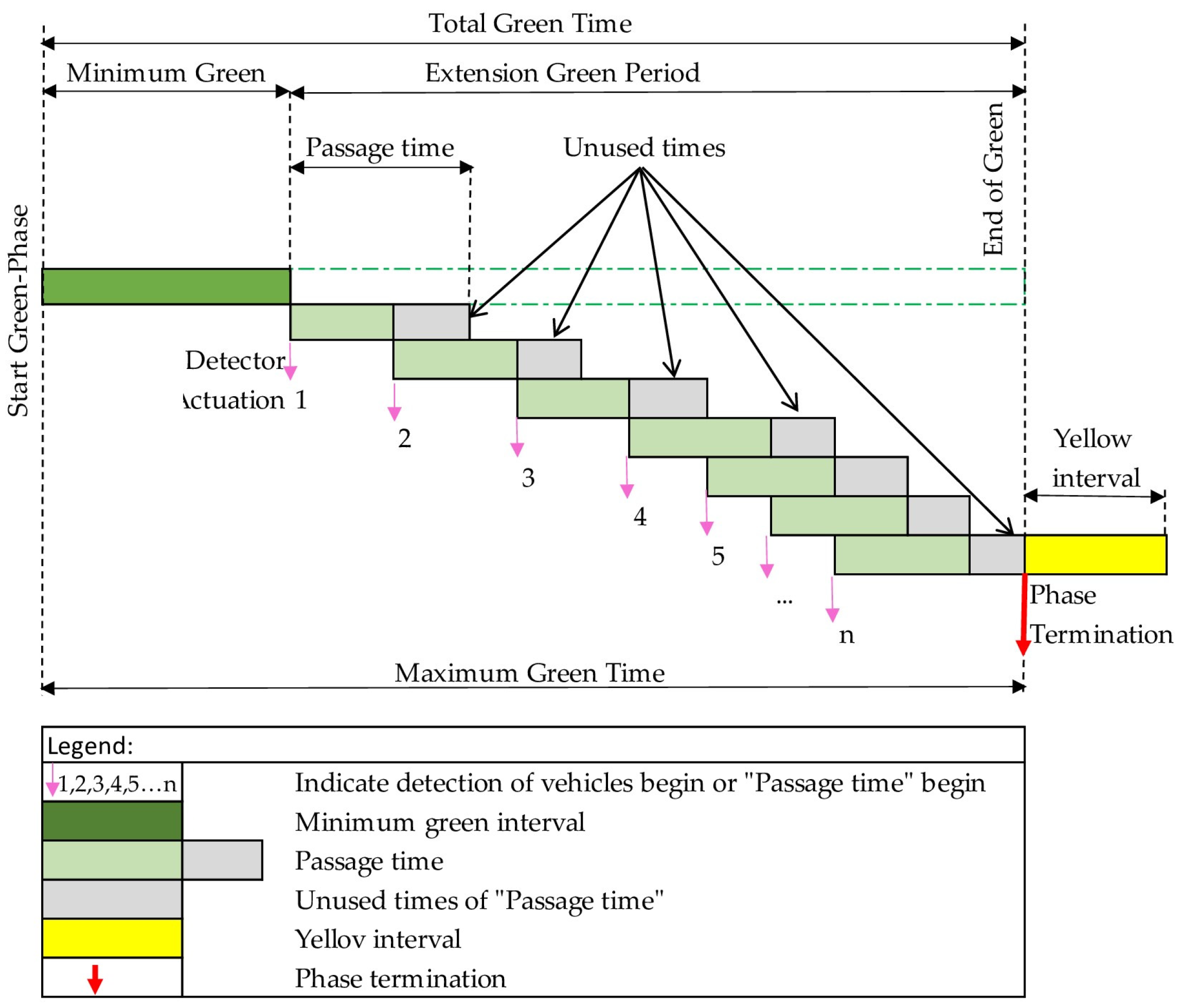
3.2.2. Semi Actuated Traffic Signal Control (SATSC)

Compared to FTSC, SATSC have the ability to respond to the presence of vehicles at intersections. SATSC consist of timed intervals called and extended to respond to traffic demands. These controllers not only have the ability to adjust the overall cycle length and green time through detector activation but also to modify the order and sequence of phases [48]. The response to these traffic flow variations generally results in reduced delays, shorter queues, and decreased travel time [42]. SATSC plans utilize information about traffic flow to allocate green times. They are equipped with detectors and necessary logic control to respond to the set demands placed on them. SATSC uses information from current demands and actions obtained from detectors within the intersection to adjust one or more aspects of signal timing based on a cycle-to-cycle basis.

The activated controllers can be programmed to accommodate: variable phase sequences (e.g., optional protected left-turn phases), variable green times for each phase, and variable cycle length induced by variable green times [49]. In general, SATSC selects phases in sequences according to their order (if there are 1, 2, 3 phases, the signal will be executed in the order 1, 2, 3), following the operational principle of ATSC’s operation. Unlike ATSC, SATSC does not automatically select phases based on traffic demand weight [31]. Signal timing is controlled and dependent on traffic demand, where detectors are positioned on the secondary roads of the intersection, while no detectors are installed on the main road. For the main road, the green interval is continuously activated, while in cases where vehicles are detected on the secondary roads, priority is then given for passage.

The green interval for the secondary directions lasts until maximum green is reached or if the detectors sense that there’s no demand for movement on the secondary roads then the transfer is made directly to the next phase. There are exceptions, and this can also be limited for a specific number of vehicles to pass. SATSC are often used in cases where there’s a need to interrupt continuous traffic flow on the main road to give priority to the secondary roads. In Figure 5, is given the algorithm and schematic representation of the SATSC operation based on the detectors placed on the secondary road [50].

Absolutely, the main task of traffic management control systems is to adjust the duration of signal phases to better suit the current traffic conditions. Just as the duration of the green interval can be determined, the duration of the red interval within the phase can also be changed. Since the focus in this paper is the selection of the optimal duration of the green interval within the phase for the given signaling group, in the following explanations are given in detail about the methods for determining the length of the green interval within the phase, as well as the adjustment of the duration of the phase itself as presented in Figure 6 and Figure 7 [51]:

• setting the predetermined initial length of the green interval and the additional passage time intervals, when necessary, results in maintaining a constant state or increasing the phase duration until the maximum is reached,
• setting the predetermined initial length of the green interval and additional passage time intervals, resulting in the predetermined duration of the phase.

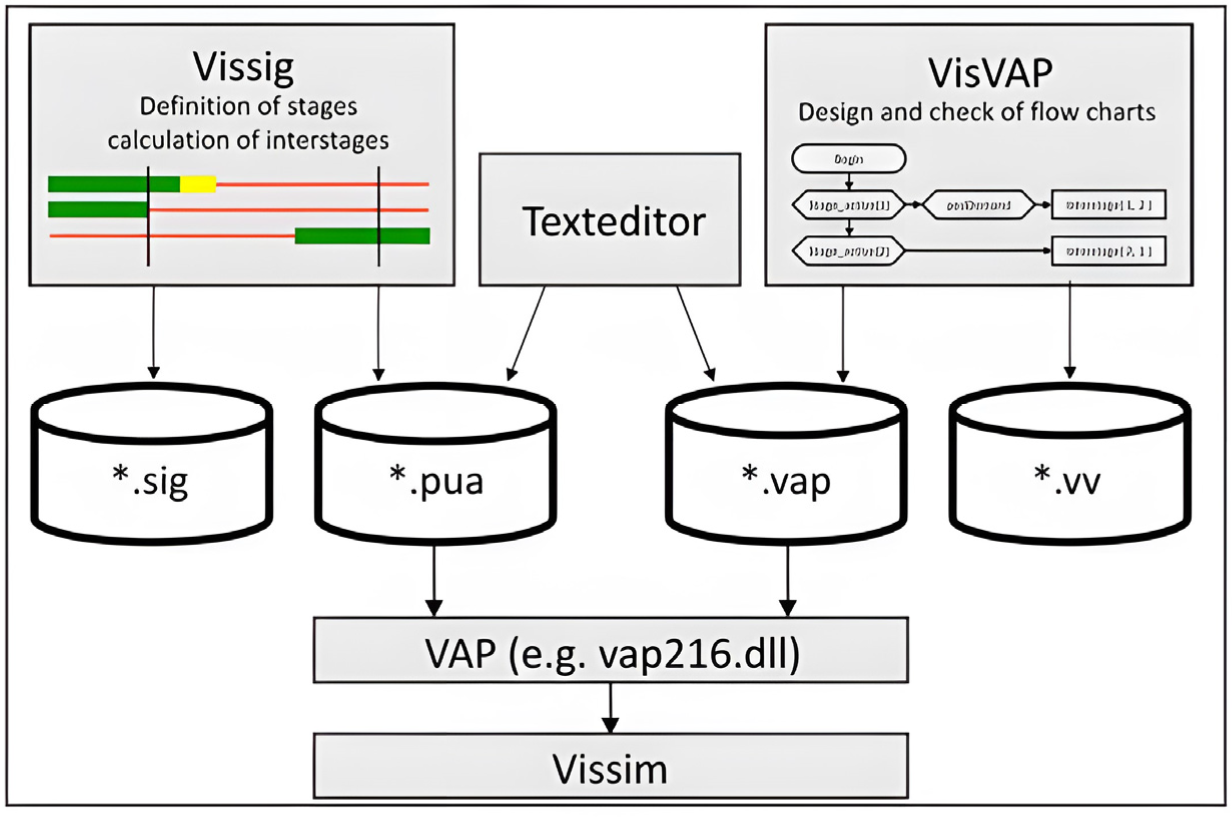
Figure 6 illustrates the continuous phase extension method, a strategy for changing phase duration based on periodic extensions when needed. Following the minimum phase duration, an evaluation occurs to determine the necessity of extension. If overloaded, shorter extensions occur, with the possibility of repeated extensions until the phase duration equals the maximum. The decision to extend the phase duration is based on the accumulated vehicle volume from the previous phase and, if necessary, incoming and outgoing traffic flow for the signal group.

Figure 6. Setting the initial determination the green interval and passage time according to demand.

Figure 6. Setting the initial determination the green interval and passage time according to demand.

Figure 7. Setting the initial determination green interval and constant and passage time addition.

Figure 7. Setting the initial determination green interval and constant and passage time addition.

In such a functioning method, the minimum and maximum duration of the phase, i.e., the duration of the green interval, is determined. It’s essential to determine the duration of the extension for the green interval after its minimum duration has expired. If it’s decided that the phase shouldn’t extend, it moves to the next phase, and if the phase extends, it transitions to the next phase only after the extension time has expired. The operation of this method is presented in Figure 7.

With both methods, it’s necessary to determine the minimum and maximum duration of the phase. In some cases, the minimum duration should not be specified, which could lead to the loss of the phase if the sufficient demand isn’t met. The maximum duration is not standardized as it depends on the characteristics of each individual intersection. Different authors provide varying values. In [40], the recommended values include up to 50% of the phase duration, while in [10], it is advised to stay within a time range of 10 to 20 s starting from the initial extension time interval.

1. The minimum green time (${\mathrm{G}}_{\min }$). In the ATSC approach, each active phase has a minimum green time, representing the smallest duration of green time allocated when a phase starts. These minimum green times are essential for each phase, including the non-active phase in a SATSC-controlled intersection. They must be set to ensure the clearance of queues. The mathematical interconnection between minimum green times and detector placement is crucial, and Equation (16) is employed to calculate minimum sums for ATSC-operated systems based on detector locations [52,53].

$$G_{min}=T_L+\left[h·Integer\left(d/x\right)\right]$$

(16)

where $G_{min}$—minimum green time (s); $T_L$—assumed start-up time loss (s); $h$—assumed saturation headway (s); $d$—distance between detectors and stop line (m); $x$—distance between stored vehicles (average 6–7 m).

2. The extended vehicle time or Unit ($\mathrm{U}$). Regarding signal operation, it serves as an allowable minimum time gap to keep the green signal active until the approaching vehicle reaches this temporal gap. Then, it is added as an additional time interval to the minimal green interval. In traffic signal control operation with actuation, the minimal green time serves to remain active and also as an extension added to the green time if there is a demand for movement in that direction. The Traffic Detector Manual [54] recommends the extension unit $U$ to be 3 s for entries with speeds equal to or less than 45 km/h.

When the speed is higher, they recommend it to be 3.5 s. For all controller types, however, the extension unit U must be equal to or greater than the passage time. The passage time is the duration it takes for a vehicle to pass from the detector to the STOP line and is calculated using Equation (17) [48].

$$U\ge P=\frac{d}{1.47·S_{15}}$$

(17)

where $U$—extended unit time (s); $P$—passage time, (s); $d$—distance from detector to stop line (m); $S_{15}$—approach speed of vehicles (km/h).

3. Maximum green time (${\mathrm{G}}_{\max }$). The critical cycle for an intersection controlled by ATSC is the cycle in which all phases reach their maximum green [55]. For intersections controlled by SATSC, the critical cycle is when the secondary road reaches the maximum green interval while the main road has the minimum green interval. The maximum green interval for each phase in ATSC and the minimum green interval for the main road in SATSC signals is determined by the maximum flow during peak hours. Every phase has a maximum green time that limits the duration of a green phase, so even if there is continuous activation, it will typically maintain the green interval. The maximum green time starts when there is a call (or activation of detectors) in a competing phase. Knowing the cycle duration ($C_i$), lost time ($L$), critical phase movements ($V_{Ci}$), and total critical movements ($V_C$), the maximum green interval can be determined by Equation (18) [48]:

$$g_i=\left(C_i-L\right)·\frac{V_{Ci}}{V_C}$$

(18)

where $C_i$—cycle length (s); $g_i$—effective green time for phase “i” (s)$; V_{Ci}$—volume in the critical lane for phase “i” (veh/h); $V_C$—sum of volumes in critical lanes (veh/h).

The calculations for cycle length and green interval can accommodate the peak hour traffic flow within the analyzed period of 15-min. These cycles are not capable of handling traffic when it exceeds the cycle’s capacity. To enhance controllers’ flexibility and accommodate larger demands, enabling cycle-by-cycle adjustments, the above equation is multiplied by 1.25 or 1.5 [48]. The resulting values represent the maximum green interval for each phase, respectively, the minimum green interval for the main road in SATSC signals. Therefore, the length of the critical cycle equals the sum of the maximum green intervals plus the green and all-red intervals, calculated using Equation (19).

$$C_c={\displaystyle \sum }_i\left(G_i+Y_i\right)$$

(19)

where $C_c$—length of the critical cycle (s); $G_i$—maximum green time for phase “i” or the minimum green time for the main road in semi-actuated signals (s); $Y_i$—sum of yellow and all-red intervals for phase “i” (s).

3.3. Tools

For creating the simulation model, additional interconnected tools can be used, namely the PTV Vissim simulation model and the supplementary modules Vissig as based-stage and VisVAP ambient graphic programming. Vissig is an additional module of PTV Vissim applied in the creation of the signal plan in the case of FTSC strategy. Through it, the rapid and adaptable creation of signaling plans is enabled based on base-staged, considered a systematic approach compared to the approach in signal groups.

VisVAP is a program that facilitates the creation of algorithms using object-oriented programming and the development of logic programs through flowcharts. It utilizes the VAP language (Vehicle Actuated Programming) as a convenient tool for creating and editing logic programs in flowchart format [56]. After developing the algorithm for a specific simulation model, the VisVAP file is initialized using the PTV Vissim program, which then executes the created simulation in the manner defined by the algorithm. The function of an individual signaling device (specified by an ASCII file with the extension *.pua) and the flowchart of the adaptive control algorithm (a file containing the code of the C++ algorithm with the extension *.vap) are integrated into the simulation model. Subsequently, the specified flowchart of the adaptive control algorithm is followed by the initiation of simulation management [57]. In Figure 8, the architecture of file functioning for building the signal control model through Vissig, VisVAP, and PTV Vissim is provided.

4. Model Development

4.1. Study Area and Data Description

The focus of the study is the magistral road M9 (Prishtina-FusheKosovo), particularly the intersection of the main road “Nene Tereza” with the secondary road “Hajrullah Zymi.” This intersection, configured in a “T” shape, is situated within the urban area of FusheKosovo. For precise simulation modeling, the intersection was designed in AutoCAD Civil 3D 2018 (*.dwg or *.dxf format) [59]. The design includes all components aligned with necessary geometric elements, detailed in Figure 9 and

Table 1. Input data related to geometric and coordinates for designing model.

Orientations	No. of Lane	Movement	Latidude	Longitude	Wide of Lane	No. of Traffic Light	Phase	Signal Group
South aproach	Lane 1	through	42.639813	21.100996	4 m	4	B	SG3
	Lane 2	through	42.639827	21.100953	3.1 m	3	B	SG3
	Lane 3	through	42.639843	21.100944	3.1 m	2	B	SG3
	Lane 4	left	42.639862	21.100934	2.1 m	5	C	SG2
East aproach	Lane 5	through	42.640049	21.101476	3.2 m	8	B	SG4
	Lane 6	through	42.640074	21.101452	3.2 m	7	B	SG4
	Lane 7	through/right	42.640113	21.101416	4.1 m	6	B	SG4
West aproach	Lane 8	left/right	42.640125	21.101085	4.6 m	1	A	SG1

.

Manual traffic flow counts conducted consistently across all lanes on Monday between period 08:00 and 09:00 a.m during peak hours, using 15-min intervals due to observed traffic flow non-linearity within the peak hour, as presented in Figure 10. At first, to consider the most realistic composition of vehicles that have circulated at this intersection, vehicles were converted into passenger car units (pce/15 min).

Subsequently, this drawing was imported into PTV Vissim software, serving as a basis for placing other necessary elements called tools by the software (links & connectors, vehicle inputs, routings, speed reductions, traffic lights, area conflicts, etc. [59]. So, the aim of this study was to examine the performance and effectiveness of intersection parameters in cases of non-linearity with varying traffic flow volumes during peak-hour time intervals. To achieve this, traffic demand quantities and the corresponding time intervals of these non-linearities have been measured for each of the scenarios, as illustrated in Figure 10.

Utilizing traffic flow data, four additional scenarios were created for distinct 15 min peak hour intervals detailed in Figure 11 See Figure 11 [60]. These traffic scenarios are categorized based on the traffic demand, into low (scenario 1, up to 500 pce/15 min), very high (scenario 2, up to 800 pce/15 min), high (scenario 3, up to 1400 pce/15 min), and moderate (scenario 4, up to 1100 pce/15 min).

The non-linearity in traffic demands vary across time intervals within the peak hour, as proposed in scenarios and summarized in Figure 11. The distribution of vehicle approaching the intersection is 10% in scenario 1, 40% in scenario 2, 30% in scenario 3, and 20% in scenario 4 of the overall traffic flow. The performance of the simulation model in PTV Vissim software was analyze separately for each scenario, considering both the FTSC SATSC strategies. A detailed analysis was conducted based on the output results.

4.2. Methodology of Model Development

Following the methodology outlined in the preceding chapter, essential parameters were analytically calculated for both the FTSC and SATSC signaling plan cases. These calculated parameters were then input into PTV Vissim software to construct the simulation models. The process involved loading the background from a file into appropriate scale of the drawing in AutoCAD. After adjusting the background and placing the intersection’s geometry, road segments were built using links, and connectors were employed to link these segments. Subsequently, desired speed limits and right-of-way rules for each conflict point in the intersection were established. As the road traverses the urban area, the microsimulation was conducted using the car-following model proposed by Wideman in 1974 (Wideman 74). This model based on driver behavior expressed by Equation (20), considering parameters such as distance and speed [61].

$$d=ax+\left(\left(b{x}_{addit}\right)+\left(b{x}_{mult}\right)·\left(z\right)\right)·\sqrt{v}$$

(20)

where $d$—safety distance between vehicles (m); $ax$—average standstill distance (m), $b{x}_{addit}$—additive part of safety distance (m); $b{x}_{mult}$—multiplicative part of safety distance (m); $z$—range value between 0 and 1, related to driver’s behavior; $v$—is free flow velocity (m/s).

The safety distance, crucial for driver deceleration when approaching or encountering stationary vehicles, incorporate both stand still and look-ahead distances. Values recommended by the Wideman 74 model, as illustrated in Figure 12, have been adopted to define these distances.

The signaling plan was created, and the traffic signal heads were placed in their respective locations, as presented in Figure 13. Each signal head corresponds to its specific signal command (signal group). Vehicles orientation was determined based on travel directions, considering the proportions of traffic flow distribution using the routing command.

Subsequently, applying the analytical calculations as outlined in Section 3, Vissig tools were employed to construct the signaling plans for the FTSC strategy, as illustrated in Figure 14. The existing state model operating under the FTSC strategy holds significant importance as the evaluation results are compared with the SATSC strategy.

These comparisons, conducted for the existing state, aims to identify improvements or deteriorations in the values of various performance measures. To build the SATSC model, the FTSC model served as a foundation, incorporate a detector on the secondary road. The signal control algorithm was then constructed using the VisVAP tools and the procedures outlined in point 3.2. The SATSC model, facilitates the detection of vehicles from the secondary road, ensuring smooth admits the heavier traffic load on the main road. The simulation process was applied to each interval and signal control method, yielding results for interpretation and assessment. To obtain results, four traffic flow scenarios with varying load demands were considered, dividing the simulation time from 0 to 3600 s, into four periods corresponding to each scenario. The scenarios are as follows: Scenario 1 (0–900 s), Scenario 2 (901–1800 s), Scenario 3 (1801–2700 s), Scenario 4 (2701–3600 s). Subsequently, both simulation models were elaborated in detail.

4.2.1. Model Developed According to the FTSC Strategy

For traffic control under the FTSC strategy, the signaling plan for the existing state has been established, comprising fixed time in 3 phases (phase A, phase B, phase C with 4 signaling groups (SG1, SG2, SG3, and SG4) depicted in Figure 15.

Notably, signal group SG1 (lane 8, left and right) is active only in Phase A, signal group SG2 (lane 4, left) is active only in Phase B, and signal group SG4 (lanes 5, 6 through and lane 7 through and right) is active in Phase C. While signaling group SG3 (lanes 1, 2, 3 through) is active in two phases, Phase B and Phase C. The analytical model adheres to the FTSC strategy, where the cycle duration and other parameters remain the same across all 4 scenarios. The cycle duration is C = 92 (s), while the green times for the phases or signal groups are specified as follows: $G_A=21 \left(\mathrm{s}\right)$, $G_{BSG2}=7 \left(\mathrm{s}\right)$, $G_{BSG3}=65 \left(\mathrm{s}\right)$, and $G_{CSG3}=65 \left(\mathrm{s}\right)$ additionally $G_{CSG4}=55 \left(\mathrm{s}\right)$. The summarized data is presented in

Table 2. Summary data for the FTSC model.

No. of Phases	Signal Group	Green Time G (s)	Yellow Time Y (s)	Red Time R (s)	Cycle Length C (s)
Phase A	SG1 (lane 8)	21	3	68
Phase B	SG2 (lane 4) and SG3 (lanes 1,2,3)	7 65	3 3	82 24	92
Phase C	SG3 (lanes 1,2,3) and SG4 (lanes 5,6,7)	65 55	3 3	24 34

.

Utilizing the VISSIG tool within PTV Vissim software, the implementation of the signal plan has been accomplished, forming the bases for constructing the simulation model, as depicted in Figure 15.

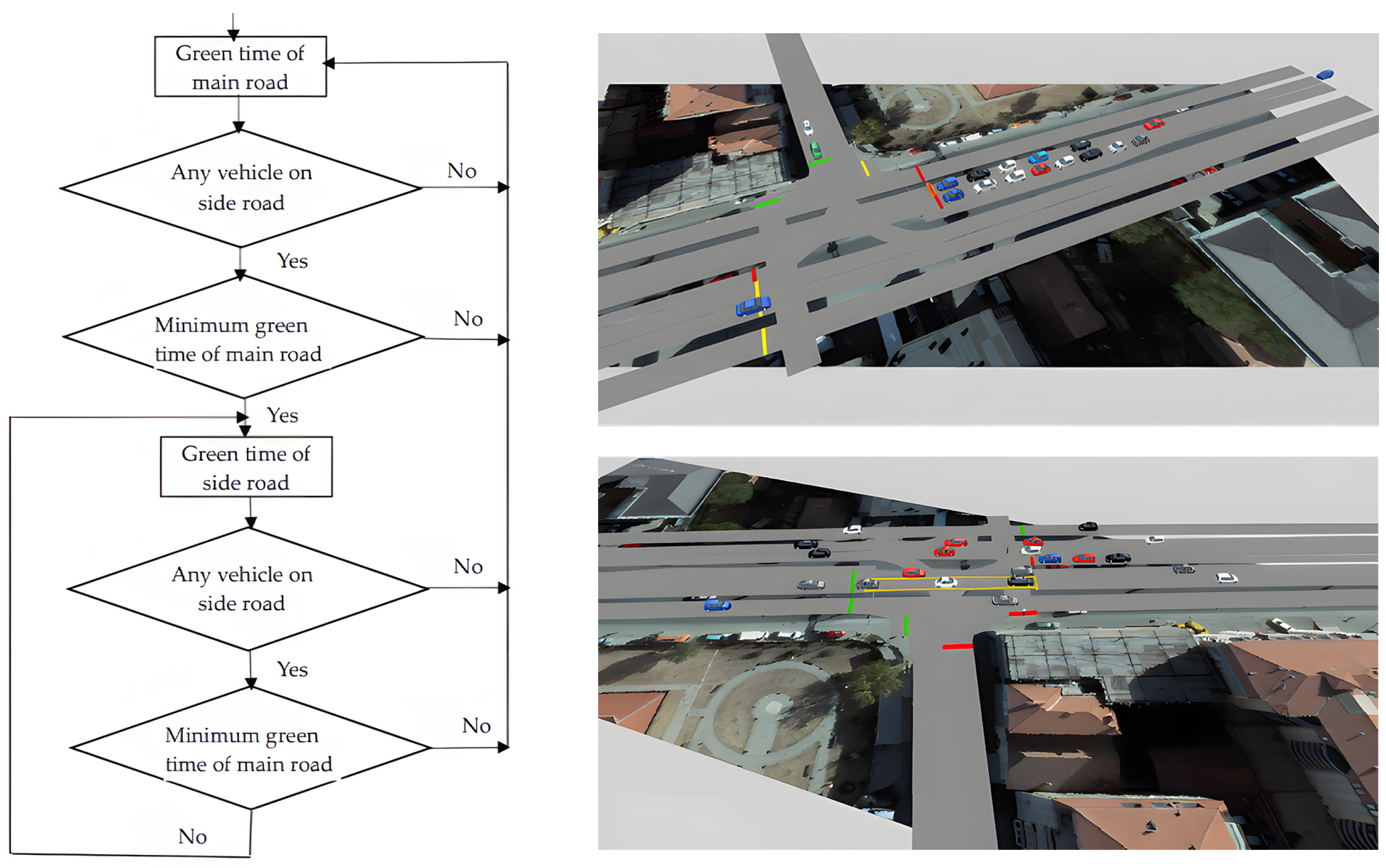
4.2.2. Model Developed According to the SATSC Strategy

The Vehicle Actuated Programming (VAP) signal, as described in point 3.2, has been applied and design the signal plan at this intersection. After placing the lanes and other necessary elements in the PTV Vissim interface, such as setting up lanes and connectors, determining the number of vehicles, placing detector on the secondary road, configuring traffic lights, creating links and connectors, the block diagram is then implemented in VisVAP tools. This block diagram is saved as a *.vap file, and from the creation of phases and interfaces, while another file is generated in *.pua format. For this model, analytical calculations have also been performed following the procedures outlined in Chapter 3.

Also here, the signal plan consists of 3 phases (Phase A, Phase B, and Phase C), encompassing four signals’ groups (SG1, SG2, SG3, and SG4) depicted in Figure 16. Observing the signal plan, signal group SG1 (lane 8, left and right) is active only in Phase A, signal group SG2 (lane 4, left) is active only in one Phase C, and signal group SG4 (lanes 5, 6 through, and lane 7 through and right) is active in Phase B. While signal group SG3 (lanes 1, 2, 3 through) is active in two phases, Phase B and Phase C.

A detector has been placed on the secondary road, specifically on the “Hajrullah Zymi” road, with no corresponding detector placed on the main road. The minimum green for SG1, respectively for the secondary road is $G_{min1}=5\left(s\right)$, sufficient to clear vehicles at the intersection. Meanwhile, the maximum green for SG2 and SG3, respectively for the main road are $G_{max2,3}=10\left(s\right)$. The optimal distance of the inductive detector, with dimensions 1.8 × 5 (m) from the stop line was determined to be approximately $d=2\left(m\right)$ based on calculations for the distance ahead. The proposed speed of vehicles on the secondary road is $S=40 \left(km/h\right)$, while the duration unit is set as $U=3\left(s\right)>P=0.57\left(s\right)$ as per the recommendations ensuring it is greater than the “passage time” from the detector to the stop line [48]. The cycle duration C fluctuates based on the traffic demand on the secondary road. When there are no vehicles on the secondary road, the minimum cycle is set to $C_{min}=26 \left(s\right)$, with only phases B and C activated. If the absence of traffic flow from the secondary road, this time is directly transferred to the green times on the main road. In situations where there is vehicle presence on the secondary road, a normal or maximum cycle of $C_{max}=34 \left(s\right)$ is applied, incorporating all three phases A, B, and C. The results are presented as in

Table 3. The summarized data for the SATSC model.

No. of Phases	Signal Group	Green Time G (s)	Yellow Time Y (s)	Unit Extension U (s)	Red Time R (s)	Cycle Length C (s)
Phase A	SG1 (lane8)	Gmin = 5	3	U = 3	R = 26
Phase B	SG3 (lanes 1,2,3) and SG4 (lanes 5.6.7)	Gmax = 10 Gmax = 10	3 3	not applicable	R = 8 R = 21	Cmin = 26
Phase C	SG3 (lanes 1,2,3) and SG2 (lane 4)	Gmax = 10 Gmax = 10	3 3	not applicable	R = 8 R = 21	Cmax = 34

.

The logical control design tools of VisVAP within the PTV Vissim software were utilized to implement the signal plan, which serve as the foundation for constructing the simulation model, as illustrated in Figure 16.

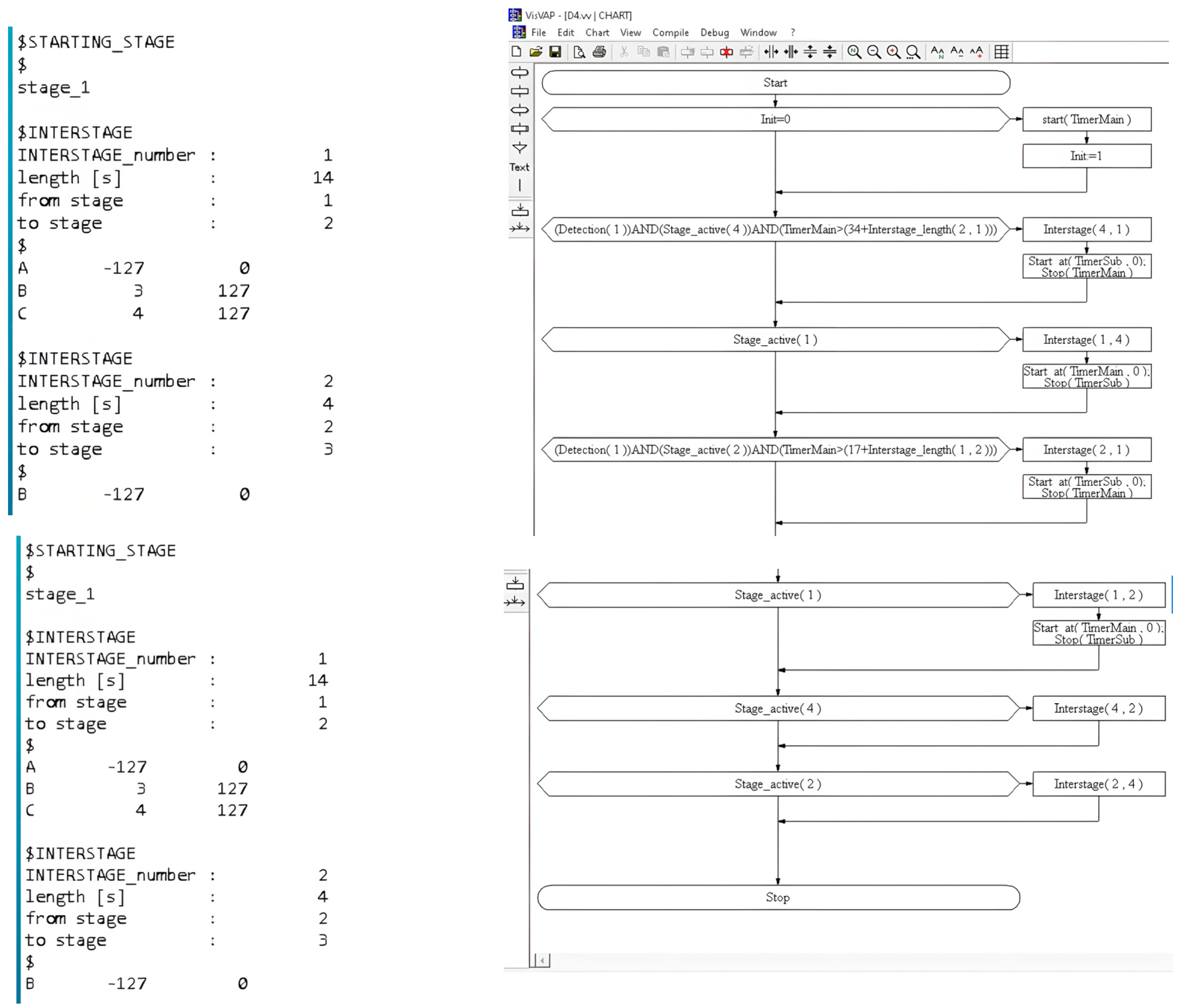
4.2.3. Logic Design Control

A *.vap file was generated for the signal program through logical control in this intersection. This section was created using development diagrams and appropriate commands within the VisVAP environment, as depicted in Figure 17. Every simulation interaction executes the logic control presented in the flowchart [62].

After creating the *.vap text file, the developed diagram is exported, now serving directly as the source file during simulation alongside the *.pua file.

5. Results and Discussion

5.1. Queue Lengths and Delay as a Performance Indicator

A set of performance indicators is employed to assess the operational quality of a signalized intersection, with queue lengths and delays being primary measures. These indicators are interrelated as output parameters. Queue lengths denotes to the number of vehicles waiting behind the stop line during a red signal phase, and delays represent the time vehicles spend in the queue. Common indicators include average queue length and average delays, expressed numerically or percentages. The queue length ratio is calculated by dividing the average queue length ($q_i)$ by its maximum value $(Q_{max})$, as defined in Equation (21) [32].

$$Queue Length ratio=\frac{1}{n}{{\displaystyle \sum }}_{i=1}^n\frac{q_i}{Q_{max}}$$

(21)

where $q_i$—represents the average queue length (m); $Q_{max}$—stands for the maximum value of the queue length (m); and $n$—refers to the number of runs from the simulation.

Delay refers to the amount of time spent to pass through an intersection—the difference between arrival time and departure time, which can be determined in various ways. Vehicle delay ratio, is calculated over the duration of the cycle length. Consequently, it’s derived by dividing the average delay $\left(d_i\right)$ by the cycle length $(C$), and it’s calculated using Equation (22) [32].

$$Vehicle Delay ratio=\frac{1}{n}{{\displaystyle \sum }}_{i=1}^n\frac{d_i}{C}$$

(22)

where $d_i$—represents the average delay of vehicles in the queue (s); $C$—cycle length (s); and $n$—refers to the number of runs from the simulation.

The microsimulation model serves as testing ground to compare the proposed strategy SATSC against FTSC. Eight specified simulation cases were conducted across four scenarios during the peak hour when traffic exhibited non-linear patterns. Simulation outputs, including performance indicators, were recorded and assessed in 15-min intervals to capture the study period. To mitigate stochastic fluctuations, average values of performance indicators were considered. Results and interpretations for the performance indicators are presented in Figure 17 and Figure 18.

5.2. Discussion of the Results Regarding Queue Length

The registered data on queue lengths for each scenario, considering the two applied strategies, are presented in Figure 18. Comparing the results, it is evident that the highest efficiency level is achieved by reducing queue length across all scenarios. There are notable improvements for each scenario during the peak hour period, with Scenario 1 indicating a decrease of 37%, Scenario 2 a decrease of 45%, Scenario 3 a decrease of 45%, and Scenario 4 a decrease of 32%. Overall, for the entire peak hour period, there is a decrease of 40%.

This demonstrates a clear trend towards traffic improvement for all scenarios during this time period when comparing the SATSC strategy against the FTSC strategy. It is evident from the results that the SATSC strategy performs better when there is high traffic flow, especially in scenarios 2 and 3, while the improvement is lower with reduced traffic flow, as seen in scenarios 1 and 4. Essentially, an increase in traffic flow results in a greater reduction in queue length, while a decrease in traffic flow leads to a smaller reduction in queue length. When analyzing each lane individually, the greatest reduction is observed in Lane 2 with a decrease of 94%, followed by Lane 3 with a decrease of 67%, then Lanes 4 and 1 with a decrease of 46%, Lane 5 with a decrease of 35%, and Lane 6 with a decrease of 32%. Meanwhile, in Lane 8 where the detector was placed, there is also a reduction in queue length with a decrease of 31%. It is worth noting that only in Lane 7, we observed an increase in queue length by 1%, a very small value compared to other directions, and it does not represent a considerably long queue for the vehicles moving in this lane.

5.3. Discussion of the Results Regarding Delays

Looking at delays as another crucial parameter in evaluation intersection performance for both strategies SATASC and FTSC, are presented graphically in Figure 19. Delays are reduced by 41% in scenario 1, by 48% in scenario 2, by 60% in scenario 3, and 56% in scenario 4, resulting in an overall reduction of 51% over the entire peak hour period. Analyzing the data from Figure 17, it is observed that with the increase in traffic flow numbers according to scenarios, there is not a proportional reduction in delays among the scenarios.

Thus, where there is a higher traffic flow (scenario 2 with 359 pce/15 min), there is a smaller reduction in delays by 48%, whereas where there is a lower traffic flow (scenario 3 with 275 pce/15 min), there is a greater reduction in delays, by 60%. When analyzing each lane individually, the most significant reduction in delays is observed in Lane 3 by 97%, followed by Lane 2 with a reduction of 95%, Lane 1 with a reduction of 88%, Lane 4 with a reduction of 82%, Lane 5 with a reduction of 29%, and Lane 6 with a reduction of 19%. In Lane 8, dedicated to left and right turn movements and where the detector was placed, we observe a reduction in delays only for left turns by 36%, while for right turns, we see an increase in delays by 17%. In Lane 7, dedicated to both straight and right-turn movements, we observe a reduction of 30% for straight movements, whereas for right turns, there is a small increase of 2%.

5.4. Comparison of Results Based on Performance Indicators

The comparison between the SATSC and FTSC strategies highlights the superior adaptability of SATSC, particularly in scenarios with higher traffic flows. In instances where traffic flows are low and approach minimal levels, the differences in control performance between the two strategies are relatively smaller concerning queue lengths but more pronounced in terms of delays. This underscores the effectiveness of SATSC in optimizing intersection performance under varying traffic conditions.

The SATSC strategy, demonstrate superior performance over the FTSC strategy throughout the peak hour, exhibiting a reduction of 39.6% in queue lengths and 51.3% in delays, as summarized in

Table 4. Average queue lengths and delays with FTSC and SATSC strategies.

Type of Control	Queue Lengths (m)	Delays (s)
FTSC	33.08	9.32
SATSC	19.31	4.50
Improvement	39.6%	51.3%

. These finding applicable specifically to the tested undersaturated operating conditions of the intersection and may not be universally generalized, even under oversaturated operating conditions.

A closer examination of the SATSC strategy reveals that the intersection performs optimally when the designated phase for the secondary road remains inactive. This case, shortens the cycle time, resulting in shorter queue lengths for vehicles on the main road. Conversely, when traffic flow from the secondary road is detected, the intersection performance declines. The cycle time increases leading to longer the queues lengths on the main road. The effectiveness of the SATSC strategy is contingent on the absence of traffic from the secondary road during certain intervals.

Similarly, in order to draw sustainable conclusions, both the advantages and disadvantages of the SATSC control strategy are presented in a summarized manner [48].

In summary, considering the aforementioned results and the suggestions provided in

Table 5. Advantages and Disadvantages of the SATSC Control Strategy.

Advantages	Disadvantages
Can be effectively used in a coordinated signaling system in a road corridor	Continuous demand and low flows from the secondary road cause excessive delays on the main road if the parameters of the maximum green interval and passage time are not appropriately set
Enables the reduction of delays on the main road during periods of light traffic	Detectors should be used on secondary roads, thus requiring their installation and continuous maintenance
They do not require detectors for the main road, and as a result, traffic flow is not compromised in their absence	Controllers are much more complex than those with fixed times, increasing maintenance costs
The main road is always supplied with the green interval, except in the presence of vehicles on the secondary road	A dedicated phase for the secondary road takes a specific minimum interval within the cycle timing whenever there is the presence of vehicles

, it’s worth emphasizing that implementing traffic control based on the SATSC as opposed to the FTSC strategy, brings significant benefits in terms of reducing overall queue lengths and delays.

6. Conclusions

In this paper, the focus has been on exploring and comparing two traffic control strategies, FTSC and SATSC, for signalized intersections. The objective was to determine which strategy yields better results in term of performance indicators at the isolation intersection, ensuring a balanced distribution of signaling plan elements, to meet the needs of all participants.

Analytical models based on FTSC and SATSC strategies were initially developed. The model designed according to the FTSC strategy has been developed based on the existing operation of traffic signal control at this intersection, while the model based on SATSC strategy is designed to calculate the minimum and maximum duration of the special green phase intended for the secondary road based on the traffic arrival rate, or its complete elimination this phase if there are no vehicles from that direction, thus transferring it directly to the next phase. Analytical models developed in this study, aimed to determine specific elements of the signal plan, including phases, intervals and cycle duration for a real intersection. These elements serve as input for construction simulation models using the microscopic software PTV Vissim, utilizing assistance tools like Vissig and VisVAP. After conducting simulation testing, derived results comparing two signal control strategies, FTSC and SATSC. The analysis focused on 15-min intervals within the peak hour across four scenarios (0–900 s, 901–1800 s, 1801–2700 s, and 2701–3600 s).

Two performance indicators, queue length and delay were considered for comparison. The results revealed a significant improvement in traffic flow, with overall reduction of queue lengths by 39.6% and reduction of vehicle delays by 51.3% at this intersection under the SATSC strategy.

The obtained results, highlight the significance of implementing design logic control using the SATSC strategy, against to FTSC strategy, for enhancing traffic sustainability. The inclusion of a detector on the secondary road effectively reduces queue lengths and time delays for vehicles at the intersection. This strategic approach not only improves traffic flow but also contributes to various additional benefits, including increased safety, reduced travel time, minimized waiting queues, lowered air pollution, decreased driver stress. As a result, the SATSC strategy aligns with the principles of traffic sustainability across multiple dimensions.

This analysis provides a valuable opportunity for the responsible authorities overseeing the road segment to explore the potential redesign of the intersection, specifically by implementing the signaling plan according to the design logic control approach. The current approach primary focused on traffic control at isolated intersections and undersaturation conditions. Recommendations for further action include conducting an analysis under oversaturation conditions and extending this logic to other intersections along the main road corridor “Nene Tereza”. Exploring the possibility of coordinating these intersections in a common network is essential. Additionally, considering other control strategies based on artificial intelligence to optimize parameters in the concrete signaling plan is advisable.

In terms of technical requirements for configuration and maintenance, the proposed design logic control relies on programming logic. Operators need to be familiar with the minimum and maximum expected values for arrival flow rate, passage time and cycle length, in order to establish “if-then” conditional instruction.

It is worth noting that a limitation of this study is absence of recorded regarding traffic flow rates for longer time periods and under various operating conditions of the intersection. This limitation could be addressed in future studies to better observe the effects of the proposed changes.

References

1. Zhao, H.; He, R.; Jia, X. Estimation and Analysis of Vehicle Exhaust Emissions at Signalized Intersections Using a Car-Following Model. Sustainability 2019, 11, 3992. [Google Scholar] [CrossRef]
2. Holguín-Veras, J.; Leal, J.A.; Sánchez-Diaz, I.; Browne, M.; Wojtowicz, J. State of the art and practice of urban freight management: Part I: Infrastructure, vehicle-related, and traffic operations. Transp. Res. Part A Policy Pract. 2018, 137, 360–382. [Google Scholar] [CrossRef]
3. Blokpoel, R.; Hausberger, S.; Krajzewicz, D. Emission optimized control and speed limit for isolated intersections. IET Intell. Transp. Syst. 2017, 11, 174–181. [Google Scholar] [CrossRef]
4. Kim, M.; Schrader, M.; Yoon, H.-S.; Bittle, J.A. Optimal Traffic Signal Control Using Priority Metric Based on Real-Time Measured Traffic Information. Sustainability 2023, 15, 7637. [Google Scholar] [CrossRef]
5. Stoilova, K.; Stoilov, T. Model Predictive Traffic Control by Bi-Level Optimization. Appl. Sci. 2022, 12, 4147. [Google Scholar] [CrossRef]
6. Ni, D. Pre-Timed Signal Timing. In Signalized Intersections-Fundamentals to Advance Systems; Springer: Cham, Switzerland, 2020; pp. 99–126. [Google Scholar] [CrossRef]
7. Truong, L.T.; Currie, G.; Wallace, M.; De Gruyter, C. Analytical approach to estimate delay reduction associated with bus priority measures. IEEE Intell. Transp. Syst. Mag. 2017, 9, 91–101. [Google Scholar] [CrossRef]
8. Mei, Z.; Tan, Z.; Zhang, W.; Wang, D. Simulation analysis of traffic signal control and transit signal priority strategies under Arterial Coordination Conditions. Simulation 2019, 95, 51–64. [Google Scholar] [CrossRef]
9. Tamannaei, M.; Fazeli, M.; Chamani Foomani Dana, A.; Mansourianfar, H. Transit Signal Priority: Proposing a Novel Algorithm to Decrease Delay and Environmental Impacts in BRT Route Intersections. Int. J. Transp. Eng. 2019, 7, 153–169. [Google Scholar] [CrossRef]
10. Traffic Signal Timing Manual-Second Edition. Chapter 5. Basic Signal Timing Procedure and Controller Parameters; Department of Transportation, Federal Highway Administration: Washington, DC, USA. Available online: https://ops.fhwa.dot.gov/publications/fhwahop08024/chapter5.htm (accessed on 6 September 2023).
11. Sustainable Urban Mobility Plan of City of Fushe Kosovo; Institute for Science and Technology (INSI Sh.p.k) and Municipality of Fushe Kosovo: Prishtine, Kosovo, 2021.
12. Fouladvand, M.E.; Sadjadi, Z.; Shaebani, M.R. Optimized Traffic Flow at a Single Intersection: Traffic Responsive Signalization. J. Phys. A Math. Gen. 2004, 37, 561–576. [Google Scholar] [CrossRef]
13. Wiering, M.; Vreeken, J.; van Veenen, J.; Koopman, A. Simulation and Optimization of Traffic in a City. In Proceedings of the IEEE Intelligent Vehicles Symposium, Parma, Italy, 14–17 June 2004; pp. 453–458. [Google Scholar] [CrossRef]
14. Chowdhury, A.; Karmakar, G.; Kamruzzaman, J.; Das, R.; Newaz, S.H.S. An Evidence Theoretic Approach for Traffic Signal Intrusion Detection. Sensors 2023, 23, 4646. [Google Scholar] [CrossRef]
15. Hao, R.; Wang, L.; Ma, W.; Yu, C. Estimating Signal Timing of Actuated Signal Control Using Pattern Recognition under Connected Vehicle Environment. Promet Traffic Transp. 2021, 33, 153–163. [Google Scholar] [CrossRef]
16. Zhu, S.; Guo, K.; Guo, Y.; Tao, H.; Shi, Q. An Adaptive Signal Control Method with Optimal Detector Locations. Sustainability 2019, 11, 727. [Google Scholar] [CrossRef]
17. Akcelik, R. Estimation of Green Times and Cycle Time for Vehicle-Actuated Signals; Transportation Research Record 1457; Sage: Atlanta, GA, USA, 1994; pp. 63–72. Available online: https://onlinepubs.trb.org/Onlinepubs/trr/1994/1457/1457-008.pdf (accessed on 22 November 2023).
18. Kim, J.T.; Courage, K.G. Evaluation and Design of Maximum Green Time Settings for Traffic-Actuated Control. Transp. Res. Rec. 1852, 2003, 246–255. [Google Scholar] [CrossRef]
19. Wu, J.; Liu, P.; Tian, Z. Operational analysis of the contraflow left-turn lane design at signalized intersections in China. Transp. Res. Part C Emerg. Technol. 2016, 69, 228–241. [Google Scholar] [CrossRef]
20. Robert, O.; Peter, W. Delay-Time Actuated Traffic Signal Control for an Isolated Intersection. Proceedings 90st Annual Meeting Transportation Research Board (TRB). 2011. Available online: https://trid.trb.org/view/1092084 (accessed on 22 November 2023).
21. Zhang, G.H.; Wang, Y.H. Optimizing minimum and maximum green time settings for traffic actuated control at isolated intersections. IEEE Trans. Intell. Transp. Syst. 2011, 12, 164–173. [Google Scholar] [CrossRef]
22. Shiri, M.J.S.; Maleki, H.R. Maximum Green Time Settings for Traffic-Actuated Signal Control at Isolated Intersections Using Fuzzy Logic. Int. J. Fuzzy Syst. 2017, 19, 247–256. [Google Scholar] [CrossRef]
23. Webster, F.V. Traffic Signal Settings; Technical Paper No. 39; Road Research Laboratory, Her Majesty Stationary Office: London, UK, 1958. [Google Scholar]
24. Akcelik, R. Time-Dependent Expressions for Delay, Stop Rate and Queue Length at Traffic Signals; Internal Report AIR367-1; Australian Road Research Board: Melbourne, Australia, 1980; Available online: https://api.semanticscholar.org/CorpusID:14676799 (accessed on 1 October 2023).
25. Highway Capacity Manual; Transportation Research Board of the National Academies: Washington, DC, USA, 2010.
26. Rathinavel, N.; Duraisamy, S.; Karuppanan, G.; Swaminathan, N. Design of Vehicle Actuated Signal using Simulation. Građevinar 2014, 66, 635–642. [Google Scholar] [CrossRef]
27. Wang, X.B.; Yin, K.; Liu, H. Vehicle actuated signal performance under general traffic at an isolated intersection. Transp. Res. Part C Emerg. Technol. 2018, 95, 582–598. [Google Scholar] [CrossRef]
28. Roess, R.; Prassas, E.S.; McShane, W.R. Traffic Engineering, 4th ed.; Pearson/Prentice Hall: Old Bridge, NJ, USA, 2011. [Google Scholar]
29. Shahgholian, M.; Gharavian, D. Advanced Traffic Management Systems: An Overview and A Development Strategy. arXiv 2018, arXiv:1810.02530. [Google Scholar]
30. Gao, J.; Shen, Y.; Liu, J.; Ito, M.; Shiratori, N. Adaptive Traffic Signal Control: Deep Reinforcement Learning Algorithm with Experience Replay and Target Network. arXiv 2017, arXiv:1705.02755. [Google Scholar]
31. Guo, Y.; Ma, J. An Improved Actuated Signal Control of Intersection Based on VISVAP. In Proceedings of the 2016 International Conference on Sensor Network and Computer Engineering, Xi’an, China, 8–10 July 2016; Atlantis Press: Dordrecht, The Netherlands, 2016; pp. 123–128. [Google Scholar] [CrossRef]
32. Maadi, S.; Stein, S.; Hong, J.; Murray-Smith, R. Real-Time Adaptive Traffic Signal Control in a Connected and Automated Vehicle Environment: Optimisation of Signal Planning with Reinforcement Learning under Vehicle Speed Guidance. Sensors 2022, 22, 7501. [Google Scholar] [CrossRef] [PubMed]
33. Toledo, T.; Balasha, T.; Keblawi, M. Optimization of Actuated Traffic Signal Plans Using a Mesoscopic Traffic Simulation. J. Transp. Eng. Part A Syst. 2020, 146. [Google Scholar] [CrossRef]
34. Tomar, I.; Indu, S.; Pandey, N. Traffic Signal Control Methods: Current Status, Challenges, and Emerging Trends. Proc. Data Anal. Manag. 2022, 1, 151–163. [Google Scholar]
35. Eom, M.; Kim, B.-I. The traffic signal control problem for intersections: A review. Eur. Transp. Res. Rev. 2020, 12, 50. [Google Scholar] [CrossRef]
36. National Academies of Sciences, Engineering, and Medicine; Urbanik, T.; Tanaka, A.; Lozner, B.; Lindstrom, E.; Lee, K.; Quayle, S.; Beaird, S.; Tsoi, S.; Ryus, P.; et al. Signal Timing Manual, 2nd ed.; The National Academies Press: Washington, DC, USA, 2015. [Google Scholar] [CrossRef]
37. Ni, D. Traffic Signal Coordination. In Signalized Intersections-Fundamentals to Advance Systems; Springer: Cham, Switzerland, 2020; pp. 291–326. [Google Scholar] [CrossRef]
38. Traffic Control Systems Handbook: Chapter 8. System Control; Department of Transportation, Federal Highway Administration: Washington, DC, USA. Available online: https://ops.fhwa.dot.gov/publications/fhwahop06006/chapter_8.htm (accessed on 5 October 2023).
39. Majstorovic, Ž.; Tišljaric, L.; Ivanjko, E.; Caric, T. Urban Traffic Signal Control under Mixed Traffic Flows: Literature Review. Appl. Sci. 2023, 13, 4484. [Google Scholar] [CrossRef]
40. Traffic Signal Timing Manual-Second Edition. Chapter 7. Local Controllers; Department of Transportation, Federal Highway Administration: Washington, DC, USA. Available online: https://ops.fhwa.dot.gov/publications/fhwahop06006/chapter_7.htm (accessed on 25 October 2023).
41. Qadri, S.S.S.M.; Gökçe, M.A.; Öner, E. State-of-art review of traffic signal control methods: Challenges and opportunities. Eur. Transp. Res. Rev. 2020, 12, 55. [Google Scholar] [CrossRef]
42. Wang, X.; Wu, X.; Liu, J. Optimization Models of Actuated Control Considering Vehicle Queuing for Sustainable Operation. Sustainability 2022, 14, 8998. [Google Scholar] [CrossRef]
43. Madrigal Arteaga, V.M.; Pérez Cruz, J.R.; Hurtado-Beltrán, A.; Trumpold, J. Efficient Intersection Management Based on an Adaptive Fuzzy-Logic Traffic Signal. Appl. Sci. 2022, 12, 6024. [Google Scholar] [CrossRef]
44. Simõesa, M.L.; Ribeiroa, I.M. Global optimization and complementarity for solving a semi-actuated traffic control problem. Procedia Soc. Behav. Sci. 2011, 20, 390–397. [Google Scholar] [CrossRef]
45. Awadallah, F. Yellow and All-red Intervals: How to Improve Safety and Reduce Delay. Int. J. Traffic Transp. Eng. 2013, 3, 159–172. [Google Scholar] [CrossRef]
46. National Academies of Sciences, Engineering, and Medicine; McGee, H.; Moriarty, K.; Eccles, K.; Liu, M.; Gates, T.; Retting, R. Guidelines for Timing Yellow and All-Red Intervals at Signalized Intersections; The National Academies Press: Washington, DC, USA, 2012. [Google Scholar] [CrossRef]
47. Ni, D. Level of Service of Traffic Signalized Intersections. In Signalized Intersections-Fundamentals to Advance Systems; Springer: Cham, Switzerland, 2020; pp. 157–178. [Google Scholar] [CrossRef]
48. Roess, R.; Prassas, E.S.; Mcshane, W. Traffic Engineering, 5th ed.; Pearson/Prentice Hall: Upper Saddle River, NJ, USA, 2021; ISBN 13: 9780137518784. [Google Scholar]
49. Chen, Z.-M.; Liu, X.-M.; Wu, W.-X. Optimization Method of Intersection Signal Coordinated Control Based on Vehicle Actuated Model. Math. Probl. Eng. 2015, 2015, 749748. [Google Scholar] [CrossRef]
50. Feng, S.; Ci, Y.; Wu, L.; Zhang, F. Vehicle Delay Estimation for an Isolated Intersection under Actuated Signal Control. Math. Probl. Eng. 2014, 2014, 356707. [Google Scholar] [CrossRef]
51. Ni, D. Controllers and Detectors. In Signalized Intersections-Fundamentals to Advance Systems; Springer: Cham, Switzerland, 2020; pp. 179–209. [Google Scholar] [CrossRef]
52. Cakici, Z.; Murat, Y.S.; Aydin, M.M. Design of an Efficient Vehicle-Actuated Signal Control Logic for Signalized Intersections. Sci. Iran. 2021, 29, 1059–1107. [Google Scholar] [CrossRef]
53. Mathew, T.V. Signalized Intersections Delay Models. Lecture Notes in Transportation System Engineering. 2017. Available online: https://www.civil.iitb.ac.in/tvm/nptel/572_Delay_A/web/web.html (accessed on 20 September 2023).
54. Manual of Uniform Traffic Control Devices for Streets and Highways 2009 Edition, including Revision 1 date May 2012, Revision 2 date May 2012, Revision 3 date July 2022. U.S Department of Transportation, Federal Highway Administration: Washington, DC, USA. Available online: https://mutcd.fhwa.dot.gov/pdfs/2009/pdf_index.htm (accessed on 10 September 2023).
55. Jin, J.; Ma, X. A group-based traffic signal control with adaptive learning ability. Eng. Appl. Artif. Intell. 2017, 65, 282–293. [Google Scholar] [CrossRef]
56. Gregurić, M.; Ivanjko, E.; Mandžuka, S. The Use of Cooperative Approach in Ramp Metering. Promet Traffic Transp. 2016, 28, 11–22. [Google Scholar] [CrossRef]
57. Pandža, H.; Vujić, M.; Ivanjko, E. A VISSIM Based Framework for Simulation of Cooperative Ramp Metering. In Proceedings of the International Scientific Conference ZIRP 2015: Cooperation Model of the Scientific and Educational Institutions and the Economy, Zagreb, Croatia, 12 May 2015; pp. 151–162. [Google Scholar]
58. PTV—Planung Transport Verkehr AG. VISVAP User Manual; PTV: Düsseldorf, Germany, 2005. [Google Scholar]
59. Ziemska, M. Exhaust Emissions and Fuel Consumption Analysis on the Example of an Increasing Number of HGVs in the Port City. Sustainability 2021, 13, 7428. [Google Scholar] [CrossRef]
60. Ziemska-Osuch, M.; Osuch, D. Modeling the Assessment of Intersections with Traffic Lights and the Significance Level of the Number of Pedestrians in Microsimulation Models Based on the PTV Vissim Tool. Sustainability 2022, 14, 8945. [Google Scholar] [CrossRef]
61. VISSIM User’s Guide. PTV (Planung Transport Verkehr) VISSIM 8.0. 2014. Available online: http://www.et.byu.edu/~msaito/CE662MS/Labs/VISSIM_530_e.pdf (accessed on 15 July 2023).
62. PTV—Planung Transport Verkehr AG. VisVAP 2.16 User Manual; PTV: Düsseldorf, Germany, 2007. [Google Scholar]
Figure 1. Integration overall structure of concept algorithm for performance indicators. Note: The asterisk (*) is a technical symbol and is the replacement for any file name or it’s a shortcut for “any file”.
Sustainability 16 02930 g001
Figure 2. Basic Operating Types of Traffic Signals Control.
Sustainability 16 02930 g002
Figure 3. Illustration of two-phase signal, intersection geometry, and phase plan.
Sustainability 16 02930 g003
Figure 4. Illustration of the change interval and clearance interval in the phase.
Sustainability 16 02930 g004
Figure 5. Flow chart of SATSC approach with detectors on the side road. Note: The lines are used for drawing the algorithm, while the colors represent the green, yellow, and red intervals according to the phase control in the traffic light by applying the PTV Vissim software (version 8, 64 bit).
Sustainability 16 02930 g005
Figure 8. Diagram of the interoperability principle among the Vissig, VisVAP, PTV Vissim [58]. Note: The asterisk (*) is a technical symbol and is the replacement for any file name or it’s a shortcut for “any file”.
Sustainability 16 02930 g008
Figure 9. Location by geoportal and design of intersection. Note: The arrows represent the directions of traffic flows, the lines depict horizontal road signaling, the green color indicates separating areas of movement directions, and the numbers (1, 2, 3, 4, 5, 6, 7, 8) represent lanes according to the geometry of the intersection.
Sustainability 16 02930 g009
Figure 10. Quarter-hour traffic volumes for all scenarios.
Sustainability 16 02930 g010
Figure 11. Observed hourly traffic volumes for all traffic scenarios.
Sustainability 16 02930 g011
Figure 12. Car-following model by Wideman 74.
Sustainability 16 02930 g012
Figure 13. Traffic model for the intersection at “Nena Tereza and Hajrullah Zymi”. Note:The colors represent the green, yellow, and red intervals according to the phase control in the traffic light by applying the PTV Vissim software (version 8, 64 bit).
Sustainability 16 02930 g013
Figure 14. Signal plan for the FTSC strategy using Vissig tools within the framework of the PTV Vissim software version 8, 64-bit.
Sustainability 16 02930 g014
Figure 15. Fixed-time signal program (a) Phase plan graph; (b) Signal plan in PTV Vissim. Note: On the left side of (a), the circles represent phases A, B, and C, while the dashed lines with arrows symbolize the transition from the current phase to the subsequent phase. Arrows with numbers (1,2,3,4,5,6,7,8) are provided within the phases to symbolize the directions of traffic flows. In (b), the graphical representation of the coordination plan according to signaling plans (SG1, SG2, SG3, and SG4) and according to the colors of the traffic light (green, yellow, red) is presented.
Sustainability 16 02930 g015
Figure 16. Semi actuated-time signal program (a) Phase plan graph; (b) Signal plan in PTV Vissim. Note: On the left side of (a), the circles represent phases A, B, and C, while the dashed lines with arrows symbolize the transition from the current phase to the subsequent phase. Arrows with full line indicate the case where there is no detection of vehicles from the secondary road; in this case, Phase C directly transitions to Phase B, thus saving time and reducing the cycle. Within the phases, arrows with numbers (1, 2, 3, 4, 5, 6, 7, 8) are provided to symbolize the directions of traffic flows. In (b), the graphical representation of the coordination plan according to signaling plans (SG1, SG2, SG3, and SG4) and according to the colors of the traffic light (green, yellow, red) is presented.
Sustainability 16 02930 g016
Figure 17. Logical control design in the *.pua and *.vap files in VisVAP for intersection.
Sustainability 16 02930 g017
Figure 18. Queue length as a function of traffic flow for four scenarios and two strategies (FTSC and SATSC), as: (a) Scenario 1 (low traffic), (b) Scenario 2 (very high traffic), (c) Scenario 3 (high traffic), and (d) Scenario 4 (moderate traffic).
Sustainability 16 02930 g018
Figure 19. Delays as a function of traffic flow for four scenarios and two strategies (FTSC and SATASC), as: as: (a) Scenario 1 (low traffic), (b) Scenario 2 (very high traffic), (c) Scenario 3 (high traffic), and (d) Scenario 4 (moderate traffic).
Sustainability 16 02930 g019