Abstract
The use of greywater heat exchangers (GHEs) is an effective way to reduce energy consumption for heating domestic water. However, the available characteristics of this type of device are often insufficient and consider only a few selected parameters of water and greywater, which results in the need to look for tools enabling the determination of the effectiveness of GHEs in various operating conditions with incomplete input data. The aim of this paper was to determine the usefulness of artificial neural networks (ANNs). For this purpose, comprehensive experimental tests were carried out on the effectiveness of the horizontal heat exchanger, taking into account a wide range of water and greywater flow rates and temperatures of these media, as well as the linear bottom slope of the unit, which allowed for the creation of a database of 32,175 results. Then, the feasibility of implementing the full research plan was assessed using ANNs. The analysis showed that the impact of the media temperatures on the heat exchanger effectiveness values obtained using ANNs is limited, which makes it possible to significantly reduce the number of necessary experiments. Adopting only three temperature values of at least one medium allowed the generation of ANN models with coefficient values R2 = 0.748–0.999 and RMSE = 0.077–1.872. In the case of the tested GHE, the slope and the flow rate of the mixed water are of key importance. However, even in the case of parameters of significant importance, it is possible to reduce the research plan without compromising the final results. Assuming five different values for each of the four input parameters (a total of 625 combinations) made it possible to generate an ANN model (R2 = 0.993 and RMSE = 0.311) with high generalization ability on the full research plan covering 32,175 cases. Therefore, the conducted analysis confirmed the usefulness of ANNs in assessing the effectiveness of GHEs in various operating conditions. The approach described in this paper is important for both environmental and economic reasons, as it allows for reducing the consumption of water and energy, which are necessary to carry out such scientific research.
1. Introduction
Sustainable energy management has become increasingly important in recent years. Borowski [1] pointed out that this resource is necessary in the context of improving living conditions and ecological development. For this reason, the implementation of efficient and cheap heat recovery systems seems to be a necessity [2,3,4], especially since basing modern energy policy solely on renewable sources may lead to periodic energy shortages [5]. Gualotuña-Gualoto et al. [6] noticed that the use of energy irretrievably lost in buildings may contribute to the decarbonization of the economy. Aleksić et al. [7] pointed out that energy recovery from otherwise wasted sources is important from the point of view of achieving a more sustainable world. Other researchers have shown that this approach is an effective way to implement a circular economy [8], especially if the heat recovery process is carried out using appropriately selected and designed devices [9].
However, the transformation towards a low-emission economy encounters a number of barriers [10], notably the attitude of potential recipients of sustainable solutions. Society’s tendency to use pro-ecological technologies is determined by both people’s personality and external factors [11]. For example, the occurrence of interrelated energy and environmental problems [12] as well as increasing legal requirements regarding the energy consumption of buildings [13] may contribute to the increasing interest in the use of energy-saving technologies. Social pressure [14], promotional campaigns [15] and the introduction of intelligent solutions [16] also play an important role in the process of implementing pro-ecological behavior. The expected results highlight the crucial significance of effective implementation. Conversely, ineffective innovations can lead to adverse environmental impacts [17], exacerbated by a scarcity of resources [18]. Therefore, the implementation of new equipment and technologies should always be preceded by a thorough analysis of the user’s needs and the requirements to be met by the solution. In the case of heat recovery technologies, the most important role will be played by the possibility of reducing the costs of energy supply to the building and improving its energy efficiency. One heat recovery technology that may find application in buildings is greywater heat recovery.
Greywater heat recovery is a sustainable technology that aims to capture and reuse the heat contained in greywater. While flowing through the heat exchanger, the thermal energy contained in the medium discharged from sanitary facilities is transferred to cold water in order to preheat it. After leaving the heat exchanger, the preheated water is fed to the domestic hot water heater and/or mixing valve.
This technology has significant potential to reduce energy consumption for domestic hot water (DHW) preparation [19], but is often met with reluctance by potential users [20]. It can find application in both residential [21] and commercial buildings [22]. Less conventional solutions are also increasingly being considered. For example, Mroziński et al. [23] analyzed solutions possible to use in a houseboat facility. The heat source is usually greywater from the shower [24], but medium discharged from other sanitary facilities are also increasingly used [25]. It is true that the amount of recoverable heat energy depends on both the type of appliance from which the greywater is discharged and the habits of the users. However, considering that the provision of thermal comfort is one of the most important aspects of building operation [26], and that thermal comfort during the use of sanitary facilities such as showers is influenced by, among other things, the flow rate and temperature of the water used [27], it can be assumed that the potential of this energy source is considerable, especially since energy consumption for DHW preparation is one of the main components of the energy balance in buildings [28], and its share of this balance is successively increasing [29].
In recent years, a number of innovative greywater heat exchangers (GHEs) have been developed. Many of these have been tested experimentally and the results of laboratory measurements were presented in scientific papers (e.g., [19,30]). In each case, the presentation of results was based on input parameter values defined by the authors, such as water and greywater flow rates through the heat exchanger or media temperatures at the unit’s input. In addition, the range of tests carried out varied considerably, making it impossible to make a clear comparison between the different units and raising questions about the sufficiency of the tests. It is clear that the execution of a full research plan is time- and cost-intensive and often unnecessary. In addition, carrying out a full research plan requires the consumption of significant amounts of water and energy, which has a negative impact on the environment. However, in the case of greywater heat exchangers, the scope of the required experimental studies has not yet been defined, the implementation of which would guarantee a full assessment of the effectiveness (ε) of the GHE for different operating conditions. Some guidance can be found in a Canadian Standards Association (CSA) document [31]. However, conducting experiments based on this guidance does not provide information on the effectiveness of the GHE at flow rates (q) other than those indicated in the standard. Moreover, it is a national standard and, consequently, is not usually considered by those carrying out tests in other countries. An additional problem arises with horizontal GHEs. While vertical heat exchangers are characterized by predetermined installation conditions, horizontal GHEs can be installed with different linear bottom slopes. Previous studies by the authors [32] showed that the slope with which the unit is installed significantly affects the hydraulic conditions in the greywater section of the GHE, and consequently also the course of the function ε = f(q).
Taking the above into account, the aim of this study was to assess the suitability of artificial neural networks (ANNs) in the effectiveness analysis of greywater heat exchangers. This tool has not yet been used in the context of using GHEs. However, it is successfully used in the analysis of other engineering systems, mainly due to the ability to adapt to various types of data and problems of varying degrees of complexity. This makes ANNs a universal and convenient tool. For example, Huang et al. [33] used ANNs in the design and geometry selection process of microchannel heat exchangers. Seenuan et al. [34] emphasized their usefulness in the structural assessment of pressurized pipes. On the other hand, Tlatelpa Becerro et al. [35] drew attention to their usefulness for predicting temperatures in the solar dryer chamber. Artificial neural networks are also widely used in civil engineering [36] and mining [37]. The examples presented prove that ANNs have significant potential for development and application in various technical fields. Although they have not yet been used to predict parameters characterizing greywater heat exchangers, the flexibility of ANNs and their ability to learn open new perspectives for their applications in the context of the use of GHEs.
This paper constitutes an important contribution to the development of greywater heat recovery technologies and to improving the capabilities of artificial intelligence applications to predict the effectiveness of GHEs. This is due to the synergistic combination of two elements in the form of experimental tests of the original design of the greywater heat exchanger and the use of artificial neural networks, which have not yet been used in the context of analyzing this type of device. Developing new and improving existing designs of greywater heat exchangers contributes to improving the effectiveness of these devices, optimizing their production costs and improving their reliability. On the other hand, the use of ANNs enables precise analysis and modeling of GHE operating parameters while limiting the consumption of environmental resources. This integrated approach opens new perspectives in the design of GHEs, potentially increasing the application possibilities of greywater heat recovery technologies.
A wide range of water and greywater flow rates through the GHE and the temperatures of these media were analyzed experimentally. The arrangement of the heat exchanger with different linear bottom slopes was also investigated. Based on the adopted variants of the dataset, the possibility of developing high accuracy ANN models for predicting the effectiveness of greywater heat exchangers over the full range of input parameters was assessed. The model is intended to derive values for the full range of data without the need for a significant number of expensive and time-consuming experiments, and may allow for significant resource savings.
2. Materials and Methods
The first stage of analysis consisted of experimental studies on the effectiveness of a prototype of the horizontal greywater heat exchanger considering a wide range of input variables covering 32,175 test cases. In the second stage of the research, predictive ANN models were developed on a limited dataset to assess the feasibility of reducing the scope of the experimental studies on the effectiveness of the horizontal GHE. From the set of experimental results, data catalogues were extracted and divided into a training set for teaching the ANN model, a validation set for tuning hyperparameters and a test set for evaluating the predictive model. The logic diagram of the research process is shown in Figure 1.
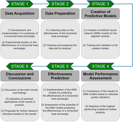
Figure 1.
Logic diagram of the research.
2.1. Experimental Research on the Effectiveness of Heat Recovery from Greywater
Experimental tests were carried out for a prototype of the horizontal heat exchanger installed on the greywater outlet from the shower. The heat exchanger was implemented in the domestic hot water preparation system integrated with the electric water heater. This type of GHEs usually does not require as much intervention and modernization of the existing building installations as vertical heat exchangers. Therefore, their implementation can be much simpler and less expensive. In addition, horizontal heat exchangers are characterized by lower requirements regarding the availability of space for installation, which is important especially in a case of existing facilities where the available space is small. Typically, this type of greywater heat exchangers is characterized by lower effectiveness of heat recovery compared to vertical units, which is why the authors focused on developing a new horizontal unit. The aim was to increase the heat exchange surface and improve effectiveness. In the future, it is planned to conduct similar analyses for other types of GHEs.
The analyzed unit was designed and constructed as a drain channel with an external rectangular cross-section with inlet and outlet for greywater. The case of the GHE was made of polyethylene. At the bottom of the greywater drain channel are four copper pipes through which the domestic cold water flows into the hot water preparation system. The copper pipes have a circular cross-section and the same diameter. The copper pipes are arranged in parallel to each other so that they form a sealed exchanger bottom separating the greywater from the cold water to be pre-heated in the horizontal GHE. According to the design concept of the heat exchanger, the cold water flows in the unit in a countercurrent manner with regard to the greywater discharged through the drain channel towards the sewage system. Table 1 shows the design parameters of the model of the horizontal GHE, while Figure 2 shows its construction.

Table 1.
Design parameters of the horizontal GHE.
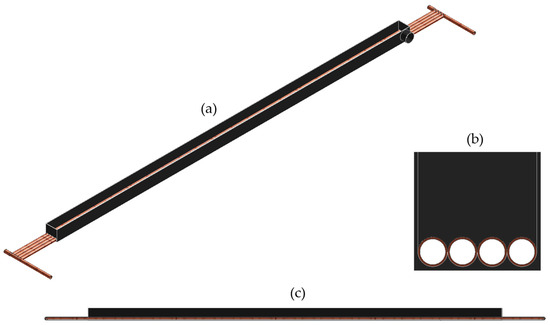
Figure 2.
Analyzed horizontal greywater heat exchanger: (a) perspective view; (b) cross-section; (c) longitudinal section.
A wide range of experimental studies of a prototype of the GHE was adopted, allowing comprehensive analyses of waste heat recovery effectiveness for various operating and design conditions, taking into account the variable linear bottom slope of the unit. The values of the input parameters are presented in Table 2.
Table 2.
The values of the input parameters adopted in the research plan.
The values of the mixed water flow rate (q) and greywater temperature (Tdw) were adopted considering the standards related to the design and operation of sanitary appliances and based on the analysis of the state of knowledge in the field of water consumption in households. In addition, the research plan included analyses covering the full range of temperature values of cold water (Tcw) entering the internal water supply system in an annual cycle. The research assumed a linear GHE bottom slope (i) in the range from 0% to 6%; however, due to significant differences observed in the results obtained for analyses carried out for a slope of 0% to 1% compared to the other values, it was decided to extend the analyses in this range of parameter i.
Laboratory tests were carried out starting from the lowest values of the input parameters (i, q, Tdw). The order in which the tests were performed for the cold water temperatures adopted in the test plan depended on the prevailing weather conditions. In the months from November to March, the tests were carried out for cold water temperatures (Tcw) ranging from 8 °C to 16 °C, and in the spring and summer months for values ranging from 17 °C to 20 °C. The research required stabilization of parameter Tcw. Depending on the water consumption in the internal water supply system, the stabilization time of this parameter ranged from a few seconds to approximately 3 min.
The experimental studies were carried out in a research laboratory located at the Rzeszow University of Technology (Poland). The ambient temperature in the room where the experimental analyses were conducted was continuously monitored and was between 23–25 °C. Three Sharky 473-type ultrasonic flowmeters were used to measure water flow rates in the DHW preparation system. Temperature measurements of water and greywater were carried out using Pt500 resistance temperature sensors. Measurement data obtained during the experimental analyses were recorded using a Simex MultiCon CMC-144 recorder. Figure 3 shows photographic documentation of the test stand.
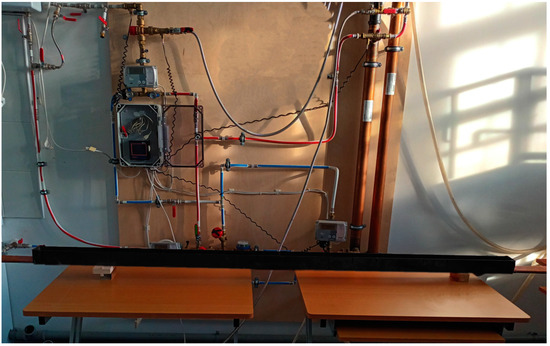
Figure 3.
Test stand with the horizontal greywater heat exchanger.
The effectiveness of the GHE prototype was determined based on the temperature values of the greywater at the inlet and outlet of the heat exchanger and taking into account the temperature values of the cold water flowing into the water section of this unit. This calculation methodology is commonly used to evaluate the effectiveness of heat recovery in heat exchangers assuming that the volume flow rate of water and greywater flowing in this unit is equal to 1:1, as was the case in this study.
2.2. Multilayer Perceptron (MLP) Neural Networks
The strength of the impact of individual input parameters on the effectiveness of greywater heat exchangers can vary considerably depending on the design case. Assessing the effectiveness of these devices is, therefore, a task that requires the analysis of multiple test scenarios, which is often time-consuming, costly and a waste of natural resources. To address these challenges, this paper investigated the validity of using artificial neural networks (ANNs), particularly multilayer perceptron (MLP) networks, as a method to reduce the number of test cases needed without compromising the accuracy of the results.
Greywater heat exchangers exhibit complex flow and heat transfer patterns that can be challenging to model with traditional rule-based methods or simpler machine learning algorithms. The inherent flexibility and efficiency of artificial neural networks in learning complex patterns and non-linearities directly from data make them an ideal choice for modeling such intricate phenomena. The authors’ assumption was to develop a model that can generalize beyond the training dataset. This is possible using artificial neural networks if they are well trained and validated. This allows for improved prediction of heat exchanger effectiveness under untested conditions.
A predictive model for the distribution of greywater heat recovery effectiveness values using horizontal GHE was developed using multilayer perceptron (MLP) artificial neural networks. This is a basic type of neural network used to model complex relationships between input and output data. It is characterized by the use of multiple layers of neurons to process data and the structure of this network consists of three main types of layers, i.e., an input layer, one or more hidden layers and an output layer. The input layer receives external data, the hidden layers process these data and the output layer generates the final result. The number of neurons in each layer can vary and is usually adapted to the specific task. A higher number of neurons and hidden layers can improve the network’s ability to model more complex relationships, but at the same time can lead to a higher risk of overfitting. Overfitting is one of the main challenges in designing and training neural networks and occurs when the model is too complex in relation to the amount and complexity of the data on which it is trained [38].
Dividing the data into training, validation and test sets is a key part of the process of designing and evaluating machine learning models, including neural networks [39]. The training set is used to teach the model, and the model parameters (e.g., weights in the neural network) are adjusted based on these data. The training set should be representative of the entire dataset so that the model can learn general relationships. The validation set, on the other hand, is used to tune the model’s hyperparameters and prevent overlearning and is not used directly to teach the model, but to evaluate its performance during training. Once the model has been taught and tuned, the test set is used for the final evaluation of model performance. The test set is completely separate from the training and validation data. The final performance of the model on the test set gives the best idea of the model’s ability to generalize and predict.
In MLP-type networks, each neuron in a layer is connected to each neuron in the next layer by weights. In each neuron of an MLP network, the input data are processed by applying an assigned activation function. The use of an activation function introduces a non-linearity that allows the MLP network to learn complex patterns in the data.
The resulting dataset from step one was used to develop sixty two datasets with selected input parameter values according to adopted variants presented in Figure 4 and Table A1 (Appendix A). These datasets, which differ in the number of cases, were then divided into three groups: a training set (70% of all data), a validation set (15% of all data) and a test set (15% of all data). The Python programming language was used to create artificial neural network models, selecting activation functions from the TensorFlow library. Of all the ANN models, those with the lowest errors were selected. To assess the performance of these models, two methodologies were employed: the root mean square error (RMSE) and the coefficient of determination (R2). RMSE is a technique that measures the average difference between the predicted (ŷi) and measured values (yi) in a dataset according to Equation (1). On the other hand, the coefficient of determination R2 is calculated by dividing the sum of squares of differences between measured (yi) and predicted values (ŷi) by the sum of squares of differences between the measured values (yi) and their average (ӯ). The value of R2 is obtained by subtracting the result of this operation from 1. The coefficient of determination (R2) is described by Equation (2) [40].
where n is the number of observations; yi is the measured value; ŷi is the predicted value; ӯ is the mean value of the dataset.
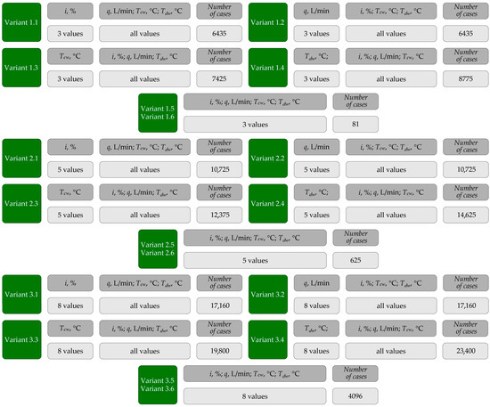
Figure 4.
The variants of datasets adopted for the development of ANN models (designations as in the text).
For the additional test set (Table A2 (Appendix B)), the difference between the observed and predicted values of the parameter ε was also calculated, as described by Equation (3). For the set of parameter difference values (∆ε), the maximum (max(∆ε)), minimum (min(∆ε)), median (med(∆ε)) and arithmetic mean (mean(∆ε)) were determined.
Adopting an additional test set (Table A2) that was not used in the process of training artificial neural network models made it possible to conduct truly predictive tests. This made it possible to evaluate how the models deal with data that are outside the range of values used during their development. This approach allows not only to verify the actual effectiveness of models in unknown data ranges, but also to identify potential limitations and areas that require further improvement.
3. Results
Research into the effectiveness of horizontal GHE was carried out in accordance with the research plan described in Section 2, which required the completion of more than 32,000 experiments. Section 3.1 presents the characteristics of the heat exchanger, which were derived from the experimental research. Section 3.2 describes the artificial neural networks that were created using the Python programming language.
To verify the reliability of the models, the predicted effectiveness values were compared with the values measured in laboratory conditions. Such a comparison allowed for a direct assessment of the ability of artificial neural networks to predict the actual effectiveness of GHEs using a limited range of input data. Thanks to this, it was possible to answer the research question whether artificial neural networks are a tool capable of precisely predicting the effectiveness of greywater heat exchangers in various operating scenarios. This analysis confirmed that the ANN models used are an effective tool for predicting effectiveness, which opens new possibilities for the design and optimization of heat exchange systems.
3.1. Characteristics of the Greywater Heat Exchanger
Due to the extensiveness of the obtained analysis results, only some of them are summarized in this subsection. Figure 5 shows the development of the effectiveness values of the heat exchanger under study as a function of the greywater and water flow rate through this unit (q) and the slope at which it is installed (i). Each plane diagram refers to different cold water (Tcw) and greywater (Tdw) temperatures at the inlet to the GHE. These values were chosen to show the development of the effectiveness of the unit at different values of the temperature difference between these media (ΔT).
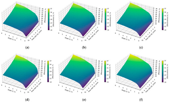
Figure 5.
Effectiveness of the tested GHE: (a) Tcw = 20 °C, Tdw = 35 °C (ΔT = 15 °C); (b) Tcw = 18 °C, Tdw = 37 °C (ΔT = 19 °C); (c) Tcw = 15 °C, Tdw = 39 °C (ΔT = 24 °C); (d) Tcw = 13 °C, Tdw = 41 °C (ΔT = 28 °C); (e) Tcw = 10 °C, Tdw = 43 °C (ΔT = 33 °C); (f) Tcw = 8 °C, Tdw = 45 °C (ΔT = 37 °C) (designations as in the text).
Experimental tests showed that the effectiveness of the greywater heat exchanger ranged from 19.37% to 36.94%, depending on the operating conditions of the system and the value of the linear bottom slope. The determined effectiveness was the higher, the lower the water and greywater flow rate through this unit. Similar conclusions with regard to horizontal heat exchangers were reached by Piotrowska and Słyś [41]. This trend is also maintained for vertical GHEs [21] and plate heat exchangers [19]. In the case of the tested heat exchanger, a reduction in flow rate from q = 10 L/min to q = 3 L/min resulted in an increase in effectiveness values of between 2.71 and 10.43 percentage points. In contrast, the median of the differences obtained for the entire test set was 8.28 percentage points. The observed reduction in effectiveness was more marked, the greater the bottom slope of the heat exchanger was. Even with a slope of i = 0.33%, the differences in effectiveness for q = 3 L/min and q = 10 L/min exceeded 6 percentage points in each case. Only when the heat exchanger was laid out without consideration of the slope (flat) did these differences not exceed 3 percentage points. However, given that such an arrangement of the unit is not advisable due to potential difficulties with gravity drainage of greywater and the resulting operational problems, it can be assumed that the effect of the flow rate of the shower head on the effectiveness of the GHE is significant. However, it should be noted that, in this case, an increase in the effectiveness of the unit does not equate to an increase in the amount of energy saved. Indeed, reducing the water flow rate from the shower head involves reducing the energy needed to heat the water, and therefore the use of energy-saving technologies will produce worse results.
The experimental study also indicated a significant effect of linear bottom slope on the effectiveness of the GHE. In the considered range of input parameter values, increasing the slope of the heat exchanger from i = 0% to i = 6% resulted in an increase in its effectiveness by a minimum of 6.2 percentage points. Such results were obtained at the highest flow rate of water and greywater in the heat exchanger (q = 10 L/min) and for the lowest temperature difference between them (Tcw = 20 °C, Tdw = 35 °C). On the other hand, an analysis of the heat exchanger’s effectiveness at the flow rate of water and greywater q = 3 L/min and for the highest temperature difference between them (Tcw = 8 °C, Tdw = 45 °C) showed that increasing the heat exchanger’s slope from the minimum to the maximum of the values considered resulted in a 13.97 percentage point increase in its effectiveness. This was the highest value recorded. In contrast, the median of the results obtained was 9.22 percentage points. The results presented prove that the effect of the slope with which the GHE is installed on its effectiveness increases as the value of the water flow rate from the shower head decreases and the temperature difference between cold water and greywater increases. It will, therefore, be most evident during the winter season. Considering that the potential for heat recovery from greywater is greatest in winter [24], the way in which the heat exchanger is installed may be crucial to the energy savings achieved and, ultimately, the potential financial savings.
Moreover, it is worth noting that in the case of the GHE under study, the increase in the slope with which it was installed resulted in an increase in its effectiveness each time. This is probably due to the design of the unit. Increasing the value of i had the effect of decreasing the thickness of the greywater layer without decreasing the heat transfer surface area. However, it should be borne in mind that further increasing the slope of the heat exchanger may lead to a situation where the greywater filling of the unit would be so small that the volume flow will be divided into several parallel volume flows. Consequently, the heat exchange surface area would be reduced, which could lead to a reduction in the effectiveness of the unit. This situation has already been observed in the case of a horizontal heat exchanger of a different design [32]. In the study of the GHE in question, larger values of i were not considered due to the limited installation conditions for this type of unit. Therefore, it can be assumed that in the case of the GHE under study, it will be advantageous to install it with the largest linear bottom slope possible under the given conditions. Significantly lower differences in the determined effectiveness of the greywater heat exchanger were observed for changes in cold water and greywater temperatures. Changing the cold water temperature, assuming constant values for the other parameters, resulted in a change in the effectiveness of the unit ranging from 0.35 to 0.80 percentage points, with the median of the determined differences being 0.52 percentage points. For greywater, it was 0.32–0.72 and 0.49 percentage points, respectively. The highest differences were recorded when the heat exchanger was laid out with the highest slope (i = 6%) and the flow rate for water and greywater was the lowest (q = 3 L/min), which was associated with achieving the highest effectiveness. Increasing the flow rate and decreasing the slope resulted in decreasing observed differences.
When analyzing the change in the temperatures of cold and greywater simultaneously, it can be seen in turn that an increase in ΔT from 15 °C (Figure 5a) to 37 °C (Figure 5f) resulted in an increase in heat exchanger effectiveness of up to 1.44 percentage points (i = 6%, q = 3 L/min). Under the different conditions (i = 0%, q = 10 L/min), this was only 0.71 percentage points. Again, these are therefore not significant differences, especially as while the cold water temperature varies significantly over the year [42], the greywater temperature does not fluctuate as much [43].
3.2. Artificial Neural Networks in Predicting the Effectiveness of Greywater Heat Exchangers
In order to test the feasibility of using machine learning methods to determine the effectiveness of the prototype of the horizontal GHE, artificial neural network models were generated. RMSE and R2 indicators (Table 3 and Table 4) were used to evaluate these models, which were determined according to Equations (1) and (2). The values of these indicators were determined for the training, validation and test sets, and additionally for a test set to check the predictive capabilities of the generated models in a wider range of datasets. For the additional test set, the difference between the observed and predicted values of the parameter ε was also calculated. Equation (3) was used for this purpose.
Table 3.
Values of R2 and RMSE for the artificial neural network models considered (designations as in the text).
Table 4.
Values of selected indicators for the additional test set (designations as in the text).
This study shows that regardless of the adopted variant, the generated artificial neural network models have a good fit to the limited dataset (Table 3). R2 coefficient values close to 1 and low RMSE values were recorded in all 3 datasets. This means that the model generalizes well to new data. This is a key aspect in machine learning, as it shows that the generated models are not overfitted to the training data and are able to make effective predictions in other cases. The highest R2 and RMSE errors were recorded for variant 1.6, which can be attributed to the relatively low number of cases in the dataset (81 cases). This confirms that the number of cases in the dataset has a direct impact on the accuracy of the model [44]. Increasing this number in each case resulted in improved model learning and generalization.
For input parameter values that fall outside the range of the dataset against which the model was trained, the use of ANNs is inherently risky and often involves high uncertainty. The selection of specific values as representative of the input parameters when training an artificial neural network has a significant impact on its ability to make accurate predictions at a later stage of analysis. The results obtained for the additional test set confirm this. Figure 6a shows the differences between the value of the R2 coefficient (Table 4) obtained for the additional test set and the maximum value of the R2 coefficient (Table 3) obtained for the dataset involved in the process of generating an artificial neural network model. This parameter was designated as ΔR2. On the other hand, Figure 6b shows the differences between the value of the RMSE (Table 4) obtained for the additional test set and the lowest value of the RMSE (Table 3), which was obtained for the set of data used to create the ANN model. This parameter was designated as ΔRMSE.
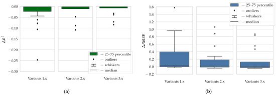
Figure 6.
Differences in the coefficients values obtained for the additional test set and the dataset involved in the process of generating the artificial neural network models: (a) ∆R2; (b) ∆RMSE (designations as in the text).
When analyzing the distribution of ∆R2 and ∆RMSE coefficient values, it can be concluded that in most variants the generated models demonstrate good generalization abilities. In other words, most models perform well at predicting results for new cases whose input parameter values are outside the range assumed when the artificial neural network models were developed. However, variants were also detected in which the phenomenon of model overfitting was noted. The highest differences between the values of ∆R2 (−0.244) and ∆RMSE (1.518) coefficients were determined for variant 1.6, which resulted from both the adoption of a very small set of input data (81 cases) and the assumption of an incorrect distribution of values in the sets of individual input parameters.
For the models with R2 value close to 1 and a low RMSE value, no high differences in ∆ε values between the predicted and actual values were recorded. Therefore, the selected models are not only effective in predicting values on average, but also demonstrate high performance in individual cases, which significantly increases the application possibilities.
When considering the data presented in Table 3 and Table 4, it was noticed that the values of the arithmetic mean and median are close to each other and in most cases they are close to 0. The symmetry of the error distribution indicates that most of the generated models do not tend to systematically overestimate or underestimate the predicted values. In practice, this means that the model can be equally useful in predicting values above and below average. This makes the resulting models more reliable and they can be used to support decision-making processes.
If an artificial neural network fits well to the dataset used for its construction and validation, but shows high errors on an additional dataset, this may indicate “overfitting”. This means that the model has adjusted too closely to the training details and cannot effectively generalize to unknown data. In practice, if this has not been previously identified by testing on additional datasets, users may unknowingly rely on a model that provides erroneous results. This, in turn, may lead to suboptimal or incorrect decisions. Therefore, it is important to always test models on a wide range of data before implementing them and using them in real scenarios, as was performed in the research described in this paper.
The research also shows that the choice of representative slope values with which the horizontal heat exchanger is installed has a decisive impact on the subsequent prediction accuracy over the full data range. The highest ability to predict the output values in the additional test set was observed when values that were in the lower and middle range of the full dataset were considered when training the ANNs (variant 1.1a, 2.1a and 3.1a). For example, taking only three representative slope values (i) of 0%, 1.5% and 3% (variant 1.1a) resulted in a maximum value of 0.901 percentage point difference between the observed and predicted heat exchanger effectiveness (max(Δε)) for the additional test set (Figure 7). Slightly less satisfactory results were obtained for variants that assumed a uniform distribution of i values in the dataset with the inclusion of outliers. On the other hand, the worst R2 and RMSE values were recorded when only values in the middle and upper range of the dataset were considered when training the ANNs. For example, variant 1.1b showed a maximum difference between observed and predicted GHE effectiveness (max(|Δε|)) of 3.706 percentage points (Figure 7). The relationships obtained are probably due to the hydraulic-energy characteristics of the heat exchanger. The relationship between the slope (i) and the effectiveness of the unit (ε) is curvilinear, and the effect of the slope (i) on the value of the parameter ε is the lower, the higher the value of i. Therefore, not including the lower range of the dataset for parameter i results in a significant overestimation of the network’s prediction in variants 1.1b (3.706 percentage points), 2.1b (3.310 percentage points) and 3.1b (3.136 percentage points). Furthermore, the significant increase in the number of cases from 6435 for variant 1.1b to 17,160 for variant 3.1b only slightly increases the performance of the network to predict the parameter ε over the full range of input data.
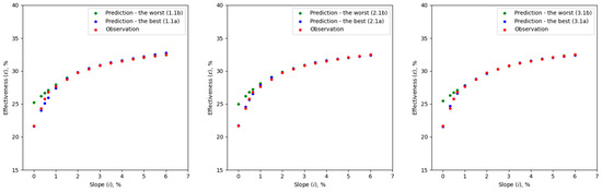
Figure 7.
Comparison between the observed and predicted values of effectiveness of the tested GHE for the selected case of additional test dataset (q = 5 L/min, Tcw = 10 °C, Tdw = 42 °C (ΔT = 32 °C)) (designations as in the text).
The selection of individual values of the mixed water flow rate (q) also significantly affects the performance of the artificial neural network model. The highest performance is observed for models 1.2a–c, 2.2d and 3.2c, for training of which a uniform distribution of the parameter q values in the dataset was assumed, considering extreme values. The adoption of only three representative values of the parameter q at the levels of 3, 5.5 and 10 L/min (variant 1.2a) made it possible to achieve high performance of the ANN model. This is confirmed by the low values of the maximum difference between the observed and predicted values of the parameter ε at 0.471 percentage points. In contrast, the lowest ANN model performance was obtained for variants 1.2f, 2.2c and 3.2d, in which flow rate (q) values lying in the middle and upper range of the full dataset were taken into account during training. The comparison of the values of the ε parameter observed and predicted by the developed artificial neural networks for selected cases from the additional test set is shown in Figure 8.
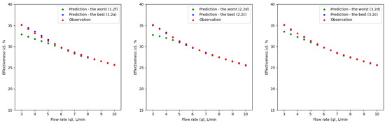
Figure 8.
Comparison between the observed and predicted values of effectiveness of the tested GHE for the selected case of additional test dataset (i = 4%, Tcw = 10 °C, Tdw = 38 °C (ΔT = 28 °C)) (designations as in the text).
For cold water temperature (Tcw) and greywater temperature (Tdw), no significant differences in R2 and RMSE values were observed between the adopted options. In all analyzed cases, there was a very good ability to predict effectiveness values (ε) over the full range of input data. This is probably due to the fact that the relationship between these parameters (Tcw, Tdw) and the effectiveness value (ε) of the greywater heat exchanger is close to a linear relationship. This is also confirmed by other studies [32,41]. In the case of near-linear relationships, artificial neural networks may have greater ability to extrapolate because the pattern they must learn to recognize and reproduce is relatively simple. In such a situation, the model has less risk of overfitting, which means that it generalizes better to unknown data, including those outside the range of the training data. Although the simplicity of the model may facilitate extrapolation, there is still a risk that predictions outside the range of the data will be less accurate. A comparison of the observed and predicted effectiveness values of the GHE for the selected case of an additional test dataset is shown for the Tdw in Figure 9 and for the Tcw in Figure 10.
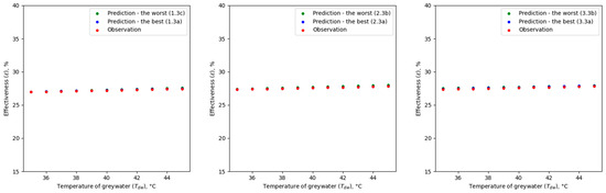
Figure 9.
Comparison between the observed and predicted values of effectiveness of the GHE for the selected case of additional test dataset (i = 1%, q = 5 L/min, Tcw = 10 °C) (designations as in the text).
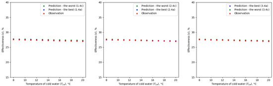
Figure 10.
Comparison between the observed and predicted values of effectiveness of the tested greywater heat exchanger for the selected case of additional test dataset (i = 4%, q = 5 L/min, Tdw = 38 °C) (designations as in the text).
Ideally, the training data should reflect the distribution of the data on which the model will be used in practice. If the training data include only a few points, it is important that the selected points reflect well the relationships between the input parameters and the predicted value. Such an assumption makes it possible to obtain high performance of the model predictions for intermediate values or even values lying outside the range of the dataset. This is confirmed by the results obtained for variants 1.5, 2.5 and 3.5, in which the distribution of input parameter values was assumed to allow the lowest error values. On the other hand, misunderstanding of the relationship between the input and output parameters of the artificial neural network model may lead to predictions with significant errors (variants 1.6 and 2.6), even with a significant number of cases taken into account (variant 3.6). This can be seen from the results in Table 3. Variant 1.5 produced significantly lower errors (R2 = 0.976, RMSE = 0.572) for the additional test set than variant 1.6 (R2 = 0.748, RMSE = 1.872). Significantly increasing the number of cases from 81 (variant 1.6) to 4096 (variant 3.6) improves the model performance (R2 = 0.927, RMSE = 1.005), but still does not exceed the model performance for variant 1.5, where only 81 cases were considered.
The determined values of the parameter ∆ε for the artificial neural network models in variants 1.5, 2.5, 3.5, 1.6, 2.6 and 3.6 are shown in Figure 11.
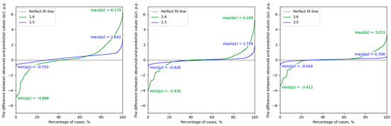
Figure 11.
The differences between the observed and predicted values of effectiveness of the tested GHE for the additional test dataset (32,175 cases) (designations as in the text).
Analysis of the ∆ε parameter values also confirms that the artificial neural network model built using the variant 3.5 dataset of 4096 cases achieves the best performance. In addition, the ANN model in variant 3.5 shows no systematic tendency to predict values that are too high or too low. This suggests that the model is well calibrated and can accurately predict actual values. Furthermore, the maximum difference between the observed and predicted value of GHE effectiveness (max(|Δε|)) is only 0.656 percentage points, and in 99.36 percent of cases the value of |Δε| is less than 0.5 percentage points, indicating the high precision of the model. Given the results obtained, the ANN model in variant 3.5 can be considered a useful tool for predicting the effectiveness (ε) value over the entire range of input data. This ability to accurately model GHE effectiveness phenomena makes the model suitable for use in engineering and research applications, where precise predictions are crucial for the optimization and design of greywater heat recovery systems.
4. Discussion
Experimental studies and analyses using artificial neural networks on the possibility of predicting the effectiveness of a greywater heat exchanger have shown that a suitable selection of representative values of the input parameters is crucial in this field. The research has shown that even with a relatively small number of cases (variant 1.5), but with appropriately selected representative values, it is possible to achieve high model effectiveness. This suggests that more important than the amount of data is their quality and representativeness for the range of values under study. This is important from a practical point of view [45], as it avoids the need for complex surveys and large datasets, which can be costly and time-consuming.
The analysis also showed that although increasing the number of input parameter values leads to an overall improvement in the quality of the artificial neural network model, it is crucial to distribute these values appropriately in the dataset. Thus, the choice of input parameters should be deliberate to reflect the diversity and specificity of the relationships under study [46].
An important finding is that the distribution and number of representative values for individual input parameters depend on the complexity of the function between these parameters and the value of the output parameter. In cases where the relationship is more complex, it becomes important to include a wider range of values so that the model can effectively learn and predict a variety of scenarios. Conversely, in situations where the correlation is simpler or closer to a linear relationship, the model can generalize effectively even from a limited number of representative data. It seems that the selection of representative values for individual parameters should be preceded by preliminary research aimed at understanding the relationship between these parameters and the output parameter [47].
The research presented in this paper is important due to the need for rational use of natural resources, considering all aspects of human existence, including scientific activity and experimental research. The laboratory analysis of the GHE involved the consumption of significant amounts of energy and water, and also necessitated an increase in the standard working time of those involved in the research, which adds an important context for discussions on the implementation of the Sustainable Development Goals (SDGs) (in particular SDG 8 “Decent Work and Economic Growth” and SDG 12 “Responsible Consumption and Production” [48]). Adopting a strategy to minimize the amount of data needed for the effective modelling and prediction of GHE effectiveness by artificial neural networks is, therefore, crucial not only from an economic point of view, but also from an environmental perspective. Working with a limited but representative number of input data and using machine learning methods provides an alternative to conducting extensive experimental studies, which can require large amounts of energy and water. This approach also reduces the carbon footprint and, consequently, the environmental impact, enabling a more sustainable and informed use of resources. These savings are important given that reducing resource consumption at each stage of the life cycle of a device or process contributes to an overall improvement in its environmental sustainability [18,49]. Therefore, intelligent data selection and optimization of research processes are of fundamental importance for sustainable development and science, and the promotion of good practices and ecological solutions in engineering and technology.
In summary, these studies provide valuable insights into the optimization of machine learning in the context of modelling the effectiveness of heat recovery systems. They highlight the importance of proper selection of input data and its representativeness for the entire range of operating conditions of the device. This approach can contribute to a more efficient and cost-effective use of artificial neural networks in engineering practice, especially in the field of energy effectiveness and heat recovery.
In considering the above, it is important to note the need to expand research on the use of ANNs in assessing the effectiveness of GHEs. Future research should consider the possibility of extending the models to include additional variables that are not usually considered in analyses. These could be, for example, data on ambient temperature, humidity, water quality and pressure or the presence of contaminants in greywater. Studies are usually carried out under laboratory conditions [19,32], so knowledge of the strength of the influence of such parameters on the effectiveness of heat recovery units is limited. Even in the case of pilot studies involving the use of wastewater of lesser quality than shower water, e.g., wastewater from commercial kitchens [50], the range of input data considered is usually restricted. This is certainly a limitation of this study, as in the case of the analyses described in this paper. However, taking into account all the parameters that could potentially influence the results of the analysis will require a significant extension of the experimental study. The combined use of ANNs and other machine learning methods, such as genetic algorithms, may also be necessary. This approach would certainly contribute to the development of more precise and comprehensive models for assessing the effectiveness of greywater heat exchangers. However, when considering the basic model input parameters, i.e., flow rate, water and greywater temperatures and the linear bottom slope of the heat exchanger, the use of artificial neural networks alone is sufficient, as evidenced by the obtained R2 and RMSE values. It can be expected that in the case of vertical units, the accuracy of the models will be even higher due to the lack of need to take into account the slope, which had the highest impact on the analysis results obtained.
Another important issue is the monitoring of heat exchangers in buildings. Integrating ANNs with Internet of Things sensors would make it possible to optimize their operation in real time, especially if adaptive artificial neural network models capable of adjusting to changing operating conditions were used. Experience with the application of similar techniques in the broadly understood construction sector [51,52] allows us to believe that the implementation of such a solution would not only maximize the achieved energy savings, but also significantly increase the reliability of the installation, e.g., by anticipating the maintenance needs of the heat recovery installation and examining its operational damage.
Further research should additionally include model sensitivity analysis, for example using SHapley Additive exPlanations (SHAP) analysis [53]. This approach has the advantage of assessing the local influence of a specific feature on a specific prediction, which will be particularly relevant for heat exchangers with variable slope effects on its effectiveness [32].
In addition to research to extend the usefulness of artificial neural networks in assessing and optimizing the performance of GHEs, there should also be a focus on the possibility of using machine learning methods for systems based on different renewable energy sources. For example, the combined use of greywater and solar or geothermal energy would reduce the consumption of conventional energy sources throughout the year. If, in addition, the cooperation between the individual components of the system were optimized using machine learning methods such as ANNs, the energy efficiency of the building could be maximized. However, the cooperation of greywater heat exchangers with other systems need not be limited to other devices based on renewable energy sources. In fact, cooperation of greywater heat exchangers with greywater recycling systems is also a promising direction for the development of GHEs. Improving the operation of such a system with ANNs would certainly contribute to increased financial savings and environmental improvements, as well as improving the efficiency of achieving the Sustainable Development Goals (including SDG6 “Clean Water and Sanitation” and SDG7 “Affordable and Clean Energy” [48]).
Based on the analyses carried out, it can also be assumed that the use of ANNs may be justified for heat exchangers of a different design and purpose. Applying this approach globally would certainly reduce the use of human and material resources.
5. Conclusions
The analysis showed that the appropriate selection of input data is crucial for the use of artificial neural networks in assessing the effectiveness of greywater heat exchangers. The precise selection of representative values for input parameters, such as the linear bottom slope of the heat exchanger, the water and greywater flow rate through the GHE, as well as the cold water and greywater temperatures, have a direct impact on the model’s ability to make accurate predictions. Based on the analysis results, it can also be noted that the temperatures of water and greywater at the inlet to the heat exchanger have the lowest impact on the quality of the models, while the slope of the unit and the media flow rate through it turned out to be of key importance. However, it should be emphasized that even in the case of the most important parameters, it is possible to limit the research plan without losing accuracy. This shows that it is not so much the quantity of the data, but rather its quality and representativeness for the range of operating conditions of the unit that are critical to achieving low prediction errors. For example, in the case of flow rate, the highest performance of the models for the tested heat exchanger was achieved when a uniform distribution of the selected q values was assumed for their training. On the other hand, when analyzing the slopes, it turned out that it is justified to take their values from the lower and middle range of the full dataset.
The analysis also points to the importance of considering the diversity of input data, which allows models to learn and predict from a wide range of research scenarios. This highlights the need for a diverse and purposeful selection of values for the various input parameters to reflect the diversity and specificity of the phenomenon under study.
Furthermore, the research demonstrates the potential of ANNs for the optimization and design of greywater heat recovery systems in engineering and research applications. Due to the high precision of the modelling, ANNs can contribute to a more efficient and cost-effective use of the technology in engineering practice.
In the context of further research, it is recommended to expand the data to include additional variables that may affect the effectiveness of GHE, such as ambient temperature, humidity or the presence of contaminants in greywater. Such an approach could contribute to even more precise models. With respect to greywater heat exchangers, it will also be beneficial to use ANNs to optimize the design of these units by identifying the most favorable geometric and material configurations. Additionally, artificial neural networks can be used to analyze the operating parameters of GHEs for the purpose of diagnosing potential problems related to their operation. Future research on the use of ANNs in issues related to GHEs should also include sensitivity analysis aimed at assessing the local impact of a given feature on a specific forecast.
Author Contributions
Conceptualization, M.S. and S.K.-O.; methodology, M.S. and S.K.-O.; software, M.S.; validation, M.S., S.K.-O. and B.P.; formal analysis, M.S., S.K.-O. and B.P.; investigation, M.S., S.K.-O. and B.P.; resources, M.S., S.K.-O. and B.P.; data curation, M.S. and B.P.; writing—original draft preparation, M.S., S.K.-O. and B.P.; writing—review and editing, S.K.-O. and B.P.; visualization, M.S. and B.P. All authors have read and agreed to the published version of the manuscript.
Funding
This research was financed by the Minister of Science and Higher Education of the Republic of Poland within the “Regional Excellence Initiative” program for the years 2024–2027 (RID/SP/0032/2024/01).
Institutional Review Board Statement
Not applicable.
Informed Consent Statement
Not applicable.
Data Availability Statement
Data are contained within this paper.
Acknowledgments
The authors would like to thank the reviewers for their feedback, which has helped improve the quality of the manuscript, and Sustainability’ staff and editors for handling this paper.
Conflicts of Interest
The authors declare no conflict of interest.
Nomenclature
| Symbol | Explanation |
| ANN | artificial neural network |
| DHW | domestic hot water |
| GHE | greywater heat exchanger |
| i | linear GHE unit bottom slope |
| max (∆ε) | maximum parameter difference value |
| mean (∆ε) | mean parameter difference value |
| med (∆ε) | median parameter difference value |
| min (∆ε) | minimum parameter difference value |
| MLP | multilayer perceptron |
| R2 | coefficient of determination |
| RMSE | root mean square error |
| SDG | sustainable development goals |
| SHAP | SHapley Additive exPlanations |
| q | mixed water flow rate |
| Tcw | cold water temperature |
| Tdw | greywater temperature |
| ӯ | mean value of the dataset |
| yi | measured value |
| ŷi | predicted value |
| ∆R | difference between R2 value for the additional test set and the maximum R2 value for the dataset used to create the ANN model |
| ∆RMSE | difference between RMSE value for the additional test set and the lowest RMSE value for the dataset used to create the ANN model |
| ∆ε | parameter difference value (difference between the measured and predicted value) |
| ε | GHE effectiveness |
Appendix A
The datasets with selected values of input parameters are presented in Table A1.
Table A1.
The datasets tested.
Table A1.
The datasets tested.
| Variants | Input Parameters | |||
|---|---|---|---|---|
| i, % | q, L/min | Tcw, °C | Tdw, °C | |
| 1.1a | 0, 1.5, 3 | all values | all values | all values |
| 1.1b | 3, 4.5, 6 | |||
| 1.1c | 0, 1, 6 | |||
| 1.1d | 0, 2, 6 | |||
| 1.1e | 0, 3, 6 | |||
| 1.1f | 1, 3, 5 | |||
| 1.2a | all values | 3, 5.5, 10 | all values | all values |
| 1.2b | 3, 6.5, 10 | |||
| 1.2c | 3, 4.5, 10 | |||
| 1.2d | 4, 6.5, 9 | |||
| 1.2e | 3, 5, 7 | |||
| 1.2f | 6, 8, 10 | |||
| 1.3a | all values | all values | 8, 14, 20 | all values |
| 1.3b | 8, 11, 14 | |||
| 1.3c | 14, 17, 20 | |||
| 1.3d | 8, 12, 20 | |||
| 1.3e | 8, 16, 20 | |||
| 1.3f | 10, 14, 18 | |||
| 1.4a | all values | all values | all values | 35, 40, 45 |
| 1.4b | 35, 37, 40 | |||
| 1.4c | 40, 42, 45 | |||
| 1.4d | 35, 38, 45 | |||
| 1.4e | 35, 42, 45 | |||
| 1.4f | 37, 40, 43 | |||
| 1.5 | 0, 1.5, 3 | 3, 5.5, 10 | 8, 14, 20 | 35, 40, 45 |
| 1.6 | 3, 4.5, 6 | 6, 8, 10 | 14, 17, 20 | 40, 42, 45 |
| 2.1a | 0, 1, 2, 3, 4 | all values | all values | all values |
| 2.1b | 2, 3, 4, 5, 6 | |||
| 2.1c | 1, 2, 3, 4, 5 | |||
| 2.1d | 0, 1.5, 3, 4.5, 6 | |||
| 2.2a | all values | 4.5, 5.5, 6.5, 7.5, 8.5 | all values | all values |
| 2.2b | 3, 4, 5, 6, 7 | |||
| 2.2c | 6, 7, 8, 9, 10 | |||
| 2.2d | 3, 4.5, 6.5, 8.5, 10 | |||
| 2.3a | all values | all values | 8, 11, 14, 17, 20 | all values |
| 2.3b | 14, 15, 17, 18, 20 | |||
| 2.3c | 8, 9, 11, 12, 14 | |||
| 2.3d | 10, 12, 14, 16, 18 | |||
| 2.4a | all values | all values | all values | 35, 37, 40, 43, 45 |
| 2.4b | 35, 36, 38, 40, 41 | |||
| 2.4c | 39, 40, 42, 44, 45 | |||
| 2.4d | 37, 38, 40, 42, 43 | |||
| 2.5 | 0, 1, 2, 3, 4 | 3, 4.5, 6.5, 8.5, 10 | 8, 11, 14, 17, 20 | 35, 37, 40, 42, 45 |
| 2.6 | 2, 3, 4, 5, 6 | 6, 7, 8, 9, 10 | 14, 16, 17, 19, 20 | 40, 41, 42, 44, 45 |
| 3.1a | 0, 0.33, 0.66, 1, 2, 2.5, 3.5, 4 | all values | all values | all values |
| 3.1b | 1, 1.5, 2.5, 3, 4, 4.5, 5.5, 6 | |||
| 3.1c | 0, 0.5, 1, 2, 3, 4, 5, 6 | |||
| 3.1d | 1, 1.5, 2, 2.5, 3, 3.5, 4, 4.5 | |||
| 3.2a | all values | 3, 3.5, 4, 4.5, 5, 5.5, 6, 7 | all values | all values |
| 3.2b | 4.5, 5, 5.5, 6, 6.5, 7, 7.5, 8 | |||
| 3.2c | 3, 4, 5, 6, 7, 8, 9, 10 | |||
| 3.2d | 6, 6.5, 7, 7.5, 8, 8.5, 9, 10 | |||
| 3.3a | all values | all values | 8, 10, 12, 13, 14, 16, 18, 20 | all values |
| 3.3b | 13, 14, 15, 16, 17, 18, 19, 20 | |||
| 3.3c | 8, 9, 10, 11, 12, 13, 14, 15 | |||
| 3.3d | 10, 11, 12, 13, 14, 15, 16, 18 | |||
| 3.4a | all values | all values | all values | 35, 37, 38, 39, 40, 42, 43, 45 |
| 3.4b | 35, 36, 37, 38, 39, 40, 41, 42 | |||
| 3.4c | 38, 39, 40, 41, 42, 43, 44, 45 | |||
| 3.4d | 36, 37, 38, 39, 40, 41, 42, 43 | |||
| 3.5 | 0, 0.33, 0.66, 1, 2, 2.5, 3.5, 4 | 3, 4, 5, 6, 7, 8, 9, 10 | 8, 10, 12, 13, 14, 16, 18, 20 | 35, 37, 38, 39, 40, 42, 43, 45 |
| 3.6 | 1, 1.5, 2.5, 3, 4, 4.5, 5.5, 6 | 6, 6.5, 7, 7.5, 8, 8.5, 9, 10 | 13, 14, 15, 16, 17, 18, 19, 20 | 38, 39, 40, 41, 42, 43, 44, 45 |
Appendix B
Additional test sets that were not used in the process of training artificial neural network models and allowed for truly predictive testing are presented in Table A2.
Table A2.
An additional test collection.
Table A2.
An additional test collection.
| Variants | Input Parameters | |||
|---|---|---|---|---|
| i, % | q, L/min | Tcw, °C | Tdw, °C | |
| 1.1a–f | all values | 5, 8 | 10, 18 | 38,42 |
| 1.2a–f | 1, 4 | all values | 10, 18 | 38,42 |
| 1.3a–f | 1, 4 | 5, 8 | all values | 38,42 |
| 1.4a–f | 1, 4 | 5, 8 | 10, 18 | all values |
| 1.5 | all values | all values | all values | all values |
| 1.6 | all values | all values | all values | all values |
| 2.1a–d | 0, 0.33, 0.5, 0.66, 1, 1.5, 2, 2.5, 3, 3.5, 4, 4.5, 5, 5.5, 6 | 5, 8 | 10, 18 | 38,42 |
| 2.2a–d | 1, 4 | 3, 3.5, 4, 4.5, 5, 5.5, 6, 6.5, 7, 7.5, 8, 8.5, 9, 9.5, 10 | 10, 18 | 38,42 |
| 2.3a–d | 1, 4 | 5, 8 | 8, 9, 10, 11, 12, 13, 14, 15, 16, 17, 18, 19, 20 | 38,42 |
| 2.4a–d | 1, 4 | 5, 8 | 10, 18 | 35, 36, 37, 38, 39, 40, 41, 42, 43, 44, 45 |
| 2.5 | all values | all values | all values | all values |
| 2.6 | all values | all values | all values | all values |
| 3.1a–d | 0, 0.33, 0.5, 0.66, 1, 1.5, 2, 2.5, 3, 3.5, 4, 4.5, 5, 5.5, 6 | 5, 8 | 10, 18 | 38,42 |
| 3.2a–d | 1, 4 | 3, 3.5, 4, 4.5, 5, 5.5, 6, 6.5, 7, 7.5, 8, 8.5, 9, 9.5, 10 | 10, 18 | 38,42 |
| 3.3a–d | 1, 4 | 5, 8 | 8, 9, 10, 11, 12, 13, 14, 15, 16, 17, 18, 19, 20 | 38,42 |
| 3.4a–d | 1, 4 | 5, 8 | 10, 18 | 35, 36, 37, 38, 39, 40, 41, 42, 43, 44, 45 |
| 3.5 | all values | all values | all values | all values |
| 3.6 | all values | all values | all values | all values |
References
- Borowski, P.F. Nexus between water, energy, food and climate change as challenges facing the modern global, European and Polish economy. AIMS Geosci. 2020, 6, 397–421. [Google Scholar] [CrossRef]
- Amanowicz, Ł.; Ratajczak, K.; Dudkiewicz, E. Recent Advancements in Ventilation Systems Used to Decrease Energy Consumption in Buildings—Literature Review. Energies 2023, 16, 1853. [Google Scholar] [CrossRef]
- Aridi, R.; Ali, S.; Lemenand, T.; Faraj, J.; Khaled, M. Innovative concept of vortex generator-equipped multi-drain heat recovery systems–Numerical study and energetic analysis. Int. J. Thermofluids 2023, 20, 100455. [Google Scholar] [CrossRef]
- Praveen Raj, P.; Kantha Shoba, M.; Ramadoss, N.; Arul, M. Enhancing desalination efficiency using waste heat from household air conditioning: A heat pipe-assisted HDH system performance analysis. Sep. Purif. Technol. 2024, 338, 126563. [Google Scholar] [CrossRef]
- Ogarek, P.; Wojtoń, M.; Słyś, D. Hydrogen as a Renewable Energy Carrier in a Hybrid Configuration of Distributed Energy Systems: Bibliometric Mapping of Current Knowledge and Strategies. Energies 2023, 16, 5495. [Google Scholar] [CrossRef]
- Gualotuña-Gualoto, D.; Martínez-Pérez, I.; Laera, R.; de Pereda, L. The Thermal Potential of Wastewater for Heating and Cooling Buildings: A Case Study of a Low Exergy Building in Madrid. Buildings 2023, 13, 2057. [Google Scholar] [CrossRef]
- Aleksić, N.; Šušteršič, V.; Jurišević, N.; Kowalik, R.; Ludynia, A. Reduction of wastewater pollution using the technologies for heat recovery from wastewater in buildings—A review of available cases. Desalin. Water Treat. 2023, 301, 242–255. [Google Scholar] [CrossRef]
- Karakutuk, S.S.; Akpinar, S.; Ornek, M.A. An Application of a Circular Economy Approach to Design an Energy-Efficient Heat Recovery System. J. Clean. Prod. 2021, 320, 128851. [Google Scholar] [CrossRef]
- Biletskyi, I.; Plankovskyy, S.; Tsegelnyk, Y.; Teliura, N.; Osinska, M. Examining the Possibility of Heat Recovery During Sanitation of Sewage Collectors. In Smart Technologies in Urban Engineering; Lecture Notes in Networks and Systems; Springer: Cham, Switzerland, 2023; Volume 88, pp. 350–362. [Google Scholar] [CrossRef]
- Ogbonna, C.G.; Nwachi, C.C.; Okeoma, I.O.; Fagbami, O.A. Understanding Nigeria’s transition pathway to carbon neutrality using the Multilevel Perspective. Carb. Neutrality 2023, 2, 24. [Google Scholar] [CrossRef]
- Madzaramba, T.H.; Zanamwe, P. User perceptions and acceptance of treated greywater reuse in low-income communities: A narrative review. J. Water Clim. Chang. 2023, 14, 4236–4244. [Google Scholar] [CrossRef]
- Dudkiewicz, E.; Fidorów-Kaprawy, N. Hybrid Domestic Hot Water System Performance in Industrial Hall. Resources 2020, 9, 65. [Google Scholar] [CrossRef]
- Fidorów-Kaprawy, N.; Dudkiewicz, E. Heating Ceiling System Efficiency in Different Climate Zones. Arch. Civ. Eng. Environ. 2023, 16, 151–161. [Google Scholar] [CrossRef]
- Stec, A. Rainwater and Greywater as Alternative Water Resources: Public Perception and Acceptability. Case Study in Twelve Countries in the World. Water Resour. Manag. 2023, 37, 5037–5059. [Google Scholar] [CrossRef]
- Dudkiewicz, E.; Ludwińska, A. Family Dwelling House Localization in Poland as a Factor Influencing the Economic Effect of Rainwater Harvesting System with Underground Tank. Sustainability 2023, 15, 10687. [Google Scholar] [CrossRef]
- González-Amarillo, C.A.; Cárdenas-García, C.L.; Mendoza-Moreno, M.A. M2M system for efficient water consumption in sanitary services, based on intelligent environment. DYNA 2018, 85, 311–318. [Google Scholar] [CrossRef]
- Wittmanová, R.; Hrudka, J.; Raczková, A.; Stanko, Š.; Škultétyová, I. Small Domestic Wastewater Treatment Plants in Rural Areas in the Conditions of the Slovak Republic. In Proceedings of the 23rd International Multidisciplinary Scientific GeoConference: Water Resources, Forest, Marine and Ocean Ecosystems, SGEM 2023, Albena, Bulgaria, 3–9 July 2023; Volume 23, pp. 141–147. [Google Scholar] [CrossRef]
- Cole, D.; Narayanan, S.; Connors, E.; Tewari, M.; Onda, K. Water stress: Opportunities for supply chain research. Prod. Oper. Manag. 2022. Available online: https://onlinelibrary.wiley.com/doi/full/10.1111/poms.13923 (accessed on 6 December 2023). [CrossRef]
- Jadwiszczak, P.; Niemierka, E. Thermal effectiveness and NTU of horizontal plate drain water heat recovery unit—Experimental study. Int. Commun. Heat Mass Transf. 2023, 147, 106938. [Google Scholar] [CrossRef]
- Kordana-Obuch, S.; Wojtoń, M.; Starzec, M.; Piotrowska, B. Opportunities and Challenges for Research on Heat Recovery from Wastewater: Bibliometric and Strategic Analyses. Energies 2023, 16, 6370. [Google Scholar] [CrossRef]
- Piotrowska, B.; Słyś, D. Analysis of the Life Cycle Cost of a Heat Recovery System from Greywater Using a Vertical “Tube-in-Tube” Heat Exchanger: Case Study of Poland. Resources 2023, 12, 100. [Google Scholar] [CrossRef]
- Schestak, I.; Spriet, J.; Styles, D.; Williams, A.P. Introducing a Calculator for the Environmental and Financial Potential of Drain Water Heat Recovery in Commercial Kitchens. Water 2021, 13, 3486. [Google Scholar] [CrossRef]
- Mroziński, A.; Grela, J.; Łowisz, M. Selected aspects of heat recovery simulation in houseboat installations. AIP Conf. Proc. 2023, 2949, 020019. [Google Scholar] [CrossRef]
- Kordana-Obuch, S.; Starzec, M. Experimental Development of the Horizontal Drain Water Heat Recovery Unit. Energies 2023, 16, 4634. [Google Scholar] [CrossRef]
- Singh, A.P.; McNabola, A. Reducing the Energy and Environmental Impact of Commercial Kitchen Water Use: Assessment of Wastewater Heat Recovery in a Grease Interceptor and Its Impact on Fat, Oil, and Grease Removal Capabilities. J. Environ. Eng. 2023, 149, 04023050. [Google Scholar] [CrossRef]
- Ratajczak, K.; Amanowicz, Ł.; Pałaszyńska, K.; Pawlak, F.; Sinacka, J. Recent Achievements in Research on Thermal Comfort and Ventilation in the Aspect of Providing People with Appropriate Conditions in Different Types of Buildings—Semi-Systematic Review. Sustainability 2023, 16, 6254. [Google Scholar] [CrossRef]
- Zhang, D.; Mui, K.W.; Wong, L.T. Establishing the Relationship between Occupants’ Thermal Behavior and Energy Consumption during Showering. Buildings 2023, 13, 1300. [Google Scholar] [CrossRef]
- Cholewa, T.; Siuta-Olcha, A.; Anasiewicz, R. On the possibilities to increase energy efficiency of domestic hot water preparation systems in existing buildings—Long term field research. J. Clean. Prod. 2019, 217, 194–203. [Google Scholar] [CrossRef]
- Amanowicz, Ł. Peak Power of Heat Source for Domestic Hot Water Preparation (DHW) for Residential Estate in Poland as a Representative Case Study for the Climate of Central Europe. Energies 2021, 14, 8047. [Google Scholar] [CrossRef]
- Soloveva, O.; Solovev, S.; Kunitsky, V.; Lukin, S.; Sinitsyn, A. Determination of the optimal heat exchanger configuration for wastewater heat recovery. E3S Web Conf. 2023, 458, 01024. [Google Scholar] [CrossRef]
- CSA B55.1-15; Test Method for Measuring Efficiency and Pressure Loss of Drain Water Heat Recovery Units. Canadian Standards Association: Mississauga, ON, Canada, 2015.
- Kordana-Obuch, S.; Starzec, M. Horizontal Shower Heat Exchanger as an Effective Domestic Hot Water Heating Alternative. Energies 2022, 15, 4829. [Google Scholar] [CrossRef]
- Huang, L.; Zou, J.; Liu, B.; Jin, Z.; Qian, J. Machine Learning Assisted Microchannel Geometric Optimization—A Case Study of Channel Designs. Energies 2024, 17, 44. [Google Scholar] [CrossRef]
- Seenuan, P.; Noraphaiphipaksa, N.; Kanchanomai, C. Stress Intensity Factors for Pressurized Pipes with an Internal Crack: The Prediction Model Based on an Artificial Neural Network. Appl. Sci. 2023, 13, 11446. [Google Scholar] [CrossRef]
- Tlatelpa Becerro, A.; Rico Martínez, R.; López-Vidaña, E.C.; Montiel Palacios, E.; Torres Segundo, C.; Gadea Pacheco, J.L. Dynamic Behavior Forecast of an Experimental Indirect Solar Dryer Using an Artificial Neural Network. AgriEngineering 2023, 5, 2423–2438. [Google Scholar] [CrossRef]
- Lagaros, N.D. Artificial Neural Networks Applied in Civil Engineering. Appl. Sci. 2023, 13, 1131. [Google Scholar] [CrossRef]
- Al-Bakri, A.Y.; Sazid, M. Application of Artificial Neural Network (ANN) for Prediction and Optimization of Blast-Induced Impacts. Mining 2021, 1, 315–334. [Google Scholar] [CrossRef]
- Chu, J.; Liu, X.; Zhang, Z.; Zhang, Y.; He, M. A novel method overcomeing overfitting of artificial neural network for accurate prediction: Application on thermophysical property of natural gas. Case Stud. Therm. Eng. 2021, 28, 101406. [Google Scholar] [CrossRef]
- Kiraga, S.; Peters, R.T.; Molaei, B.; Evett, S.R.; Marek, G. Reference Evapotranspiration Estimation Using Genetic Algorithm-Optimized Machine Learning Models and Standardized Penman–Monteith Equation in a Highly Advective Environment. Water 2024, 16, 12. [Google Scholar] [CrossRef]
- Nourani, V.; Fard, M.S. Sensitivity analysis of the artificial neural network outputs in simulation of the evaporation process at different climatologic regimes. Adv. Eng. Softw. 2012, 47, 127–146. [Google Scholar] [CrossRef]
- Piotrowska, B.; Słyś, D. Variant analysis of financial and energy efficiency of the heat recovery system and domestic hot water preparation for a single-family building: The case of Poland. J. Build. Eng. 2023, 65, 105769. [Google Scholar] [CrossRef]
- Żukowski, M. Experimental determination of the cold water temperature at the inlet to solar water storage tanks. Therm. Sci. Eng. Prog. 2020, 16, 100466. [Google Scholar] [CrossRef]
- Dudkiewicz, E.; Ludwińska, A.; Rajski, K. Implementation of greywater heat recovery system in hospitals. E3S Web Conf. 2019, 116, 00018. [Google Scholar] [CrossRef]
- Afram, A.; Janabi-Sharifi, F.; Fung, A.S.; Raahemifar, K. Artificial neural network (ANN) based model predictive control (MPC) and optimization of HVAC systems: A state of the art review and case study of a residential HVAC system. Energy Build. 2017, 141, 96–113. [Google Scholar] [CrossRef]
- Pal, J.; Chakrabarty, D. Effects of input/output parameters on artificial neural network model efficiency for breakthrough contaminant prediction. Water Supply 2021, 21, 3614–3628. [Google Scholar] [CrossRef]
- Lee, J.; Yang, D.; Yoon, K.; Kim, J. Effects of Input Parameter Range on the Accuracy of Artificial Neural Network Prediction for the Injection Molding Process. Polymers 2022, 14, 1724. [Google Scholar] [CrossRef] [PubMed]
- Liu, X.; Tian, S.; Tao, F.; Yu, W. A review of artificial neural networks in the constitutive modeling of composite materials. Compos. B. Eng. 2021, 224, 109152. [Google Scholar] [CrossRef]
- United Nations (UN). The Sustainable Development Goals Report 2021; United Nations: New York, NY, USA, 2021. [Google Scholar]
- Stec, A.; Słyś, D. New Bioretention Drainage Channel as One of the Low-Impact Development Solutions: A Case Study from Poland. Resources 2023, 12, 82. [Google Scholar] [CrossRef]
- Spriet, J.; Singh, A.P.; Considine, B.; Murali, M.K.; McNabola, A. Design and Long-Term Performance of a Pilot Wastewater Heat Recovery System in a Commercial Kitchen in the Tourism Sector. Water 2023, 15, 3646. [Google Scholar] [CrossRef]
- Baduge, S.K.; Thilakarathna, S.; Perera, J.S.; Arashpour, M.; Sharafi, P.; Teodosio, B.; Shringi, A.; Mendis, P. Artificial intelligence and smart vision for building and construction 4.0: Machine and deep learning methods and applications. Autom. Constr. 2022, 141, 104440. [Google Scholar] [CrossRef]
- Matetić, I.; Štajduhar, I.; Wolf, I.; Ljubic, S. Improving the Efficiency of Fan Coil Units in Hotel Buildings through Deep-Learning-Based Fault Detection. Sensors 2023, 23, 6717. [Google Scholar] [CrossRef]
- Dinmohammadi, F.; Han, Y.; Shafiee, M. Predicting Energy Consumption in Residential Buildings Using Advanced Machine Learning Algorithms. Energies 2023, 16, 3748. [Google Scholar] [CrossRef]
Disclaimer/Publisher’s Note: The statements, opinions and data contained in all publications are solely those of the individual author(s) and contributor(s) and not of MDPI and/or the editor(s). MDPI and/or the editor(s) disclaim responsibility for any injury to people or property resulting from any ideas, methods, instructions or products referred to in the content. |
© 2024 by the authors. Licensee MDPI, Basel, Switzerland. This article is an open access article distributed under the terms and conditions of the Creative Commons Attribution (CC BY) license (https://creativecommons.org/licenses/by/4.0/).