Advancing Traffic Simulation Precision and Scalability: A Data-Driven Approach Utilizing Deep Neural Networks

Abstract

In traditional traffic simulation studies, vehicle behavior has typically been modeled using complex analytical frameworks, which often struggle to encompass the full range of variables affecting vehicle operations. Addressing this gap, our research introduces an innovative data-driven framework for traffic simulation that incorporates human driving data into its decision-making processes. This enables the modeling of diverse vehicle behaviors by taking into account both vehicle-specific characteristics and environmental factors. At the core of this framework are two advanced deep neural networks, convolutional long short-term memory and convolutional gated recurrent unit, which underpin our vehicle traffic simulation model. Utilizing datasets from the Next Generation Simulation project, specifically the I-80 and US-101 road sections, our study further evaluates the framework’s performance through single-step continuous prediction, as well as transferability tests, employing the TransMSEloss function to optimize prediction accuracy. Our findings reveal that the proposed data-driven model significantly outperforms traditional models, achieving an exceptional accuracy of 97.22% in training and 95.76% in testing. Notably, in continuous prediction, our model maintains an 89.57% accuracy up to the fifth step, exceeding the traditional framework’s 82.82% by 5% to 10% at each step. Time cost analysis indicates that while the data-driven framework’s advantages are more pronounced in large-scale simulations, it also demonstrates strong transferability, with a 93.48% accuracy on diverse datasets, showcasing its applicability across different traffic scenarios. This study not only highlights the potential of deep learning in traffic simulation, but also sets a new benchmark for accuracy and scalability in the field.

1. Introduction

In the realm of transportation systems, marked by their increasing complexity and the growing prevalence of shared mobility options, the escalating issues of traffic congestion, accidents, and environmental pollution are becoming more pronounced [1,2,3]. Within the United States, congestion costs surged from USD 166 billion in 2014 to USD 190 billion in 2019 [4,5,6]. Traffic simulation has emerged as a pivotal tool to address these multifaceted challenges, encompassing concerns such as traffic congestion, safety, pollution, and energy consumption [7,8,9]. In pursuit of enhancing safety, a calibrated microscopic traffic simulation model forms the foundation for a safety assessment model [10,11]. Furthermore, Hishikawa et al. [7] conducted an evaluation of the safety of mixed traffic, which includes pedestrians and personal motor vehicles, by analyzing the impact of geometric and traffic conditions using a traffic simulation model.

The research and development of software pertaining to traffic simulation constitute a vital component of the broader field of traffic simulation research [12,13,14]. Among the notable simulation models, CORridor SIMulation (CORSIM) stands out as a microscopic traffic simulation model tailored for the analysis of both highways and urban roads. It utilizes the safety distance model as its car-following (CF) model [8,15]. In contrast, Simulation of Urban Mobility (SUMO) (Version 1.19.0), an open-source and multimodal microscopic traffic simulation software, adopts the Gipps extension model as its CF model [9]. Park et al. [16] conducted a comprehensive study on the calibration and validation of a microscopic traffic simulation model, using the Verkehr In Städten—SIMulationsmodell (VISSIM) simulation model to analyze a coordinated actuated signal system. It is noteworthy that traffic simulation software fundamentally relies on specific and intricate analytical mathematical models to facilitate vehicle traffic simulation [17]. However, these analytical models have inherent limitations, as they can only account for a limited number of factors influencing driving behavior [18,19]. Furthermore, these models simulate different traffic behaviors in isolation, leading to significant disparities between simulation outcomes based on analytical models and real-world observations [20,21,22]. Wastavino et al. pointed out the inherent limitations of analytical models in fully capturing the intricacies of driving behavior [23]. Subsequently, Toledo et al. developed and tested a driving behavior framework that integrates both the CF model and the lane-changing (LC) model. However, this data-driven framework’s complexity and inflexibility posed challenges [24].

Conversely, some scholars have proposed an alternative approach, contending that various driving behavior models are inherently embedded within vehicle trajectories. They suggest that the challenging task of concurrently modeling the CF and LC models can be supplanted by directly modeling vehicle trajectories [25,26,27]. For instance, Tomar employed a multilayer perceptron to predict the future trajectories of discrete vehicles [28]. Cui et al. developed a deep convolutional neural network designed for predicting future vehicle trajectories [29]. Additionally, Zhang et al. introduced the hybrid retraining constrained (HRC)–long short-term memory (LSTM) method for the simultaneous prediction of vehicle trajectories [30]. While extensive research on trajectory prediction has validated its effectiveness in simultaneously modeling CF and LC behaviors, its simulation efficiency in large-scale networks remains questionable. This is primarily because such models often focus on predicting the trajectory of individual vehicles without adequately considering the future movements of surrounding vehicles. Consequently, in large-scale networks, particularly within high-density traffic flows, simulating the entire traffic scenario requires iterating over all vehicles in the scene, significantly reducing computational efficiency. Given these challenges, the development of a simulation framework that can efficiently simulate all vehicles in a large-scale network scenario while maintaining high computational efficiency is essential.

As for the realm of data-driven machine learning models, Li et al. proposed a multivariate ensembles-based hierarchical linkage strategy, fusing the benefits of multivariate ensembles model into the hierarchical linkage technique [31]. By employing the developed hierarchical leveling strategy for system decomposition and the subsequent application of the mapping engine model for synchronous mapping of subsystem outputs, this approach facilitates the construction of a multi-level system reliability framework. Abdelaty et al. developed and evaluated seven data-driven modeling techniques, spanning both machine learning and statistical models, providing a comprehensive analysis of each model’s applicability [32].

Addressing the aforementioned limitations, we present a novel data-driven traffic simulation framework that leverages deep neural networks as the core data-driven kernel model. This framework integrates human driving experience data for decision-making, allowing it to simultaneously model various vehicle driving behaviors while considering both vehicle-specific factors and environmental influences. Distinct from conventional model-driven methods and individual vehicle trajectory prediction approaches, our framework concurrently simulates the entire road segment, rather than sequentially simulating vehicles on an individual basis. To facilitate a comprehensive comparison, we also establish model-driven and trajectory prediction frameworks and calibrate their respective parameters. To enhance the training efficiency and performance capabilities of the data-driven framework, we introduce improvements to the mean-squared error (MSE) loss function and introduce TransMSELoss as the designated loss function during network training. In single-step prediction, the data-driven framework demonstrates impressive accuracy, achieving 97.22% on the training set and 95.76% on the test set. Moreover, in the context of five consecutive prediction experiments, the data-driven framework consistently outperforms the model-driven framework, exhibiting accuracy levels that are generally 5% to 10% higher. Furthermore, we delve into the scalability of the simulation frameworks, exploring promising avenues for enhancing their capabilities. Additionally, we conduct a thorough transferability analysis, revealing that the data-driven framework exhibits exceptional transferability. This work carries significant implications, not only in terms of achieving more accurate simulations, but also in enabling the feasibility of large-scale road network simulations.

The rest of this paper is organized as follows: Section 2 introduces the frameworks of model-driven traffic simulation, trajectory prediction, and the data-driven traffic simulation. Section 3 describes the parameter configuration of the model. Section 4 gives the comparison results and verifies the performance of the frameworks. Section 5 studies the transferability of the model. Section 6 concludes the paper.

2. Methodology

In this section, we delve into the specifics of our framework, starting with the model-driven traffic simulation framework and its submodel, trajectory prediction, which utilizes the LSTM architecture. Following that, we provide an in-depth exploration of the structure of the data-driven traffic simulation framework, including a detailed breakdown of the two neural network structures employed within it.

2.1. Model-Driven Traffic Simulation Framework

Typically, existing traffic simulation software relies on various microscopic traffic simulation models to simulate vehicle operations. These models encompass the simulation of vehicle driving behavior, with a primary focus on CF and LC models, as outlined by Toledo [33].

2.1.1. CF Model

CF models, such as the intelligent driver model (IDM), elucidate how a vehicle tracks the movements of the preceding vehicle within a single lane. These models employ analytical formulas to characterize the vehicle’s longitudinal behavior on the roadway. CF models find extensive applications across various domains, including microscopic traffic simulation, analysis of driving behaviors, capacity assessment, and traffic safety [34]. For the purpose of this paper, we designate the IDM as our benchmark model [35].

The IDM is depicted by Equations (1) and (2), offering a unified description of the transition of vehicles from free-flow conditions to congested flow. This model assesses the vehicle’s following motion by considering the acceleration induced by a range of social forces, encompassing both the driving force and resistance. The driving force emanates from the driver’s psychological inclination to attain a desired speed, while the resistance arises from the influence of the leading vehicle on the following vehicle.

$$a_i\left(t\right)=A_i\left[1-{\left(\frac{v_i\left(t\right)}{v_f}\right)}^{\delta }-{\left(\frac{{s_i}^{\ast }\left(t\right)}{s_i\left(t\right)}\right)}^2\right]$$

(1)

$${s_i}^{\ast }\left(t\right)=s_0+s_1\sqrt{\frac{v_i\left(t\right)}{v_f}}+T_i{v}_i\left(t\right)+\frac{v_i\left(t\right)[v_i\left(t\right)-v_{i-1}\left(t\right)]}{2\sqrt{A_i{b}_i}}$$

(2)

where $a_i\left(t\right)$ is the acceleration of the vehicle i at time t; $A_i$ denotes the maximum acceleration of the vehicle i; $v_i\left(t\right)$ is the speed of the vehicle i at time t; $v_f$ is the free-flow speed; $\delta$ stands for the acceleration index $(\delta >0)$; $s_i\left(t\right)$ is the spacing between the vehicle i and the vehicle $i-1$; ${s_i}^{\ast }\left(t\right)$ is the desired spacing; $s_0$ is the stationary safety distance; $s_1$ is a coefficient usually taken as 0; $T_i$ is the safe time headway; and $b_i$ is the comfortable deceleration.

2.1.2. LC Model

The Minimizing Overall Braking Induced by Lane changes (MOBIL) model utilizes vehicle acceleration to define the utilities and assesses LC decisions by comparing the utilities of the current lane and the locally affected vehicles on the target lane, both before and after the LC behavior [36].

The MOBIL model posits that acceleration serves as an intuitive indicator of the lane selection’s effectiveness. Essentially, driver decision-making in LC involves selecting a lane that offers the prospect of improved acceleration. According to the MOBIL model, the decision-maker evaluates the benefits derived from changing lanes and the potential ramifications for vehicles in both the original lane and the target lane during the LC process. Lane changes are considered necessary only when they contribute to enhancing the overall system’s utilities.

The MOBIL model also emphasizes that the main safety concerns are centered around the LC vehicle and the following vehicles in the target lane while executing the lane change maneuver. If either the following vehicle or the LC vehicle experiences substantial deceleration, it indicates an unsafe lane change. As a result, it is imperative to ensure that the safety criteria specified in Equation (5) are met during the lane change process.

$$U_{\alpha ,k}=a_{\alpha ,k}$$

(3)

$${\widehat{a}}_{\alpha }-a_{\alpha }+p\left({\widehat{a}}_{\widehat{f}}-a_{\widehat{f}}+{\widehat{a}}_f-a_f\right)>\mathsf{\Delta }a+a_{bias}$$

(4)

$${\widehat{a}}_{\widehat{f}}=f\left(v_{\widehat{f}},v_{\alpha },{\widehat{s}}_{\widehat{f}}\right)>-b_{safe}$$

(5)

where $a_{\alpha ,k}$ is acceleration calculated according to the CF model when vehicle $\alpha$ selects lane k; $U_{\alpha ,k}$ is the utility of vehicle $\alpha$ selecting lane k; ${\widehat{a}}_{\alpha }$ is the following acceleration of the vehicle $\alpha$ after the vehicle $\alpha$ changes lanes, while $a_{\alpha }$ is the following acceleration of the vehicle $\alpha$ before changing lanes; ${\widehat{a}}_{\widehat{f}}$ and $a_{\widehat{f}}$ are the acceleration of the following vehicle on the target lane after and before vehicle $\alpha$ changing lane; ${\widehat{a}}_f$ and $a_f$ are the acceleration of the following vehicle on the original lane after and before vehicle $\alpha$ changing lane; ${\widehat{s}}_{\widehat{f}}$ denotes the gap between the vehicle $\alpha$ and the following vehicle on the traget lane; $p\in [0,1]$ is the altruistic factor; $\mathsf{\Delta }a$ is the threshold for the improvement of the overall utility of changing lanes; $a_{bias}$ is the asymmetric lane change parameters; and $-b_{safe}$ denotes the absolute value of the maximum deceleration to ensure driving safety.

2.2. Trajectory Prediction

LSTM, a specialized recurrent neural network, possesses the ability to effectively model time series data with extended time intervals and autonomously ascertain the optimal prediction time lag [37]. The utilization of LSTM networks enables us to grasp human driving trajectory data, consequently facilitating the advancement and amalgamation of CF and LC vehicle driving behaviors [38,39].

LSTM diverges from traditional recurrent neural networks by governing the cell state via three inherently parameterized control gates: the forget gate, input gate, and output gate.

In the initial stage of LSTM, the determination of which information to discard from the cell state is orchestrated by a sigmoid layer known as the “forget gate”. This gate takes inputs, namely $h_{(t-1)}$ (the previous output) and $x_t$ (the current input), and produces an output value ranging between 0 and 1 for each element in the cell state $c_{(t-1)}$ (the previous state). A value of 1 signifies complete retention of the information, while a value of 0 signifies its complete removal.

• Forget Gate:

  $$f_t=\sigma \left(W_{xf}{x}_t+W_{hf}{h}_{t-1}+W_{cf}{c}_{t-1}+b_f\right)$$

  (6)

The subsequent stage involves determining which information to retain in the cell state, a process divided into two distinct steps. Firstly, a sigmoid layer referred to as the “input gate” determines which values should be updated. Following that, a hyperbolic tangent (tanh) layer constructs a candidate vector, denoted as $c_t$, which will be incorporated into the state of cells.

• Input Gate:

  $$i_t=\sigma \left(W_{xi}{x}_t+W_{hi}{h}_{t-1}+W_{ci}{c}_{t-1}+b_i\right)$$

  (7)

  $$c_t=f_t{c}_{t-1}+i_{t}tanh\left(W_{xc}{x}_t+W_{hc}{h}_{t-1}+b_c\right)$$

  (8)

Finally, the output of the cell unit is controlled by the output gate.

• Output Gate:

  $$o_t=\sigma \left(W_{xo}{x}_t+W_{ho}{h}_{t-1}+W_{co}{c}_t+b_{\mathrm{o}}\right)$$

  (9)

  $$h_t=o_{t}tanh\left(c_t\right)$$

  (10)

  where $\sigma$ is the sigmoid layer; $x_t$ is the input data at time t; $f_t$, $i_t$, and $o_t$ are the forget gate, input gate, and output gate at time t, respectively; $h_t$ is the hidden state; $c_t$ is the cell state at the time t; W is the weight coefficient; and b is the bias.

2.3. Data-Driven Traffic Simulation Framework

2.3.1. ConvLSTM

Convolutional long short-term memory (ConvLSTM), a derivative of LSTM, introduces a pivotal modification by replacing the full connection layer in LSTM with a convolutional layer and altering the model’s input from a vector to a 3D tensor. This adjustment is made to address the inherent limitation of LSTM in encoding spatial information during the state transition process [40,41]. The equation expression for ConvLSTM is as follows, where the ∗ symbol signifies the convolution operator, and the ∘ symbol denotes the Hadamard product:

$$\left\{\begin{array}{l}{i}_t=\sigma \left(W_{xi}\ast x_t+W_{hi}\ast h_{t-1}+W_{ci}\circ c_{t-1}+b_i\right)\\ f_t=\sigma \left(W_{xf}\ast x_t+W_{hf}\ast h_{t-1}+W_{cf}\circ c_{t-1}+b_f\right)\\ c_t=f_t\circ c_{t-1}+i_t\circ tanh\left(W_{xc}\ast x_t+W_{hc}\ast h_{t-1}+b_c\right)\\ o_t=\sigma \left(W_{xo}\ast x_t+W_{ho}\ast h_{t-1}+W_{co}\circ c_t+b_o\right)\\ h_t=o_t\circ tanh\left(c_t\right)\end{array}\right.$$

(11)

where $\sigma$ is the sigmoid layer; $x_t$ is the input data at time t; $f_t$, $i_t$, and $o_t$ are forget gate, input gate, and output gate at time t, respectively; $h_t$ is the hidden state; $c_t$ is the cell state at the time t; W is the weight coefficient; and b is the bias.

2.3.2. ConvGRU

Gated recurrent unit (GRU), another variation of LSTM, distinguishes itself by dispensing with the memory unit present in LSTM and consolidating the input gate and forget gate into a single component called the “update gate” [42,43]. Additionally, it introduces the “reset gate”, amalgamating the advantages of recurrent units with convolutional layers. This enables convolutional gated recurrent unit (ConvGRU) to effectively process sequential data that possess spatial dimensions. By regulating the information flow through the reset gate, ConvGRU enhances its capability to capture and model long-range dependencies, rendering it a valuable asset across diverse domains. With each new input, the reset gate determines whether to clear the previous state, while the update gate governs the extent to which new information is incorporated into the state.

$$\left\{\begin{array}{l}{z}_t=\sigma \left(W_{xz}\ast x_t+W_{hz}\ast h_{t-1}\right)\\ r_t=\sigma \left(W_{xr}\ast x_t+W_{hr}\ast h_{t-1}\right)\\ h_t^{\prime }=f\left(W_{xh}\ast x_t+r_t\circ \left(W_{hh}\ast h_{t-1}\right)\right)\\ h_t=\left(1-z_t\right)\circ h_t^{\prime }+z_t\circ h_{t-1}\end{array}\right.$$

(12)

where $\sigma$ is the sigmoid layer; f is the activation; $x_t$ is the input data at time t; $z_t$, $r_t$, $h_t$, and $h_t^{\prime }$ are update gate, reset gate, memory state, and new information at time t, respectively; and W is the weight coefficient.

2.3.3. Data-Driven Traffic Simulation Framework Structure

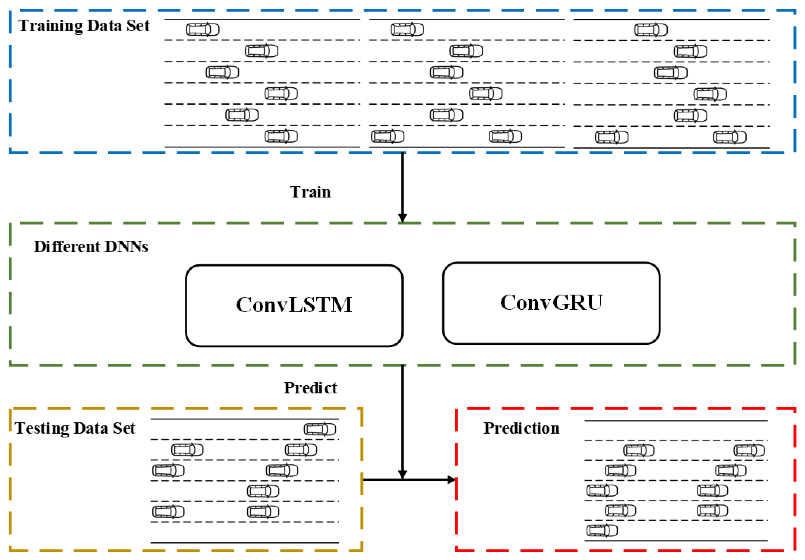
The structure of the data-driven traffic simulation framework is depicted in Figure 1. In this framework, training data comprise vehicle traffic data from a particular scenario, with the central component consisting of various deep neural networks. Once these neural networks are trained, they are utilized to make predictions on the test set.

3. Case Study

3.1. Data Preparation

Considering that the core of the data-driven traffic simulation framework relies on deep neural networks, a significant volume of training data is essential. Since the dataset utilized is the Next Generation Simulation (NGSIM) dataset, which contains trajectory data and employs ConvLSTM and ConvGRU, the training input comprises high-dimensional tensor data.

Our approach involved segmenting and organizing the trajectory data from NGSIM, subsequently converting them into temporally sequenced, road section-based vehicle data, following the methodology outlined by Montanino and Punzo [44]. Each individual cell in this dataset is defined with a length of 2 m, matching the width of a typical lane. It is important to note that the concept of an individual cell inherently incorporates a tolerance within the accuracy rate calculation, given that achieving ‘perfect alignment’ in predictions is challenging. Specifically, a tolerance margin is established around the predicted vehicle cell, accommodating slight deviations from the precise position and yet still recognizing the prediction as accurate. This built-in tolerance acknowledges the practical limitations of prediction models and accommodates the variability encountered in real-world driving conditions. As a result, we obtained an extensive dataset composed of serialized cells, with 75% allocated for training and 25% for testing.

It is important to emphasize that the NGSIM dataset is extracted from traffic videos and may contain noise, particularly in the speed and acceleration data segments. However, we exclusively leveraged the location data within the NGSIM dataset, ensuring that our experiments remained largely unaffected by such noise.

3.2. Model Parameters’ Setting

3.2.1. Model-Driven Traffic Simulation Parameters’ Configuration

As highlighted earlier, the CF model employed in our model-driven traffic simulation is the IDM. To align IDM’s performance with real-world traffic behaviors, it is imperative to calibrate its parameters accurately. Our calibration methodology leverages the Particle Swarm Optimization (PSO) method, renowned for its efficacy in optimizing non-linear and complex functions. This approach involves initializing a swarm of particles, each representing a potential solution—in this case, a set of IDM parameters. These particles explore the solution space, guided by their own best-known positions and the swarm’s overall best-known position. Furthermore, the PSO method introduces a stochastic element, enhancing the algorithm’s exploration capabilities across the solution space. By dynamically adjusting trajectories based on both personal and global bests, complemented by this random factor, our approach mitigates the risk of premature convergence on suboptimal solutions. We utilized detailed trajectory data from the I-80 road section within the NGSIM dataset as the basis for calibration, allowing us to refine the IDM parameters for enhanced fidelity to observed vehicle behaviors. The calibration process iteratively adjusts the IDM parameters to minimize the deviation between the model’s predictions and the actual vehicle trajectories observed in the dataset. The outcomes of this meticulous calibration procedure are detailed in

Table 1. Calibrated parameters in IDM and MOBIL.

Parameters	Value
a	$0.73$ m/s2
$v_0$	33.3 m/s
$s_0$	2.5 m
T	1.6 s
b	$1.67$ m/s2
p	$0.1$
$\mathsf{\Delta }a$	$0.1$ m/s2
$b_{safe}$	4 m/s2
$a_{bias}$	$0.3$ m/s2

. For the sake of clarity and simplicity in presentation, we have chosen to omit the subscripts of parameters in our discussion and analysis.

3.2.2. Trajectory Prediction Model Parameters’ Configuration

We conducted orthogonal experiments on various LSTM parameters, including batch size, the number of neurons in the hidden layer, dropout rate, and training epochs. The specific parameter settings are outlined in

Table 2. Calibrated parameters in the LSTM.

Parameter	Description	Values
Input dimension	Dimensions of the input layer	2
Output dimension	Dimensions of the output layer	2
Historical length	Number of past frames (0.1 s)	40
Hidden layer number	Number of LSTM layer	1
Neuron in the hidden layer	Number of neurons in the hidden layer	80
Dropout rate	The rate of neurons applied at dropout	0.2
Training epochs	Number of training update	1000
Batch size	Number of training samples sent into the network each time	16
Loss function	The function to calculate loss	MSELoss
Activation function	The function to map input and output	Sigmoid
Optimizer	The function to find the optimal solution	Adam

.

3.2.3. Data-Driven Traffic Simulation Parameters’ Configuration

As ConvLSTM and ConvGRU are pivotal to the architecture of our data-driven framework, fine-tuning their parameters is crucial for maximizing model efficacy. To navigate the intricate process of determining the optimal configuration for these deep neural networks, we embarked on a series of orthogonal experiments, which were specifically designed for systematic parameter tuning. During this phase, we divided our dataset into distinct training and validation sets. This division was crucial for evaluating various parameter combinations and their impact on model performance within the validation set, thereby optimizing the selection of parameters while avoiding the risk of overfitting. Following the identification of the optimal parameter set from the calibration phase, we further validated the models’ efficacy and generalization ability using a completely separate testing set.

The calibration process for ConvLSTM, in particular, required a nuanced approach due to its unique architecture, which combines convolutional layers with LSTM units to capture spatial–temporal patterns in traffic data. By varying the aforementioned parameters, we sought to identify a configuration that balances the model’s ability to learn complex dependencies with computational efficiency. The optimal parameters identified through these experiments, which strike a delicate balance between learning capacity and generalization ability, are meticulously cataloged in

Table 3. Calibrated parameters in ConvLSTM and ConvGRU models.

Parameter	Description	Values
Input dimension	Dimensions of the input layer	(6, 31)
Output dimension	Dimensions of the output layer	(6, 31)
Historical length	Number of past frames (0.1 s)	40
Hidden layer number	Number of ConvLSTM layer	1
Neuron in the hidden layer	Number of neurons in the hidden layer	80
Dropout rate	The rate of neurons applied at dropout	0.2
Training epochs	Number of a training update	5000
Batch size	Number of training samples sent into the network each time	16
Loss function	The function to calculate loss	TransMSELoss
Activation function	The function to map input and output	Sigmoid
Optimizer	The function to find the optimal solution	Adam

.

During the calibration phase, it became apparent that standard loss functions such as MSELoss and Structural Similarity Index Measure (SSIM) were inadequate for our model training objectives. Neither could fully capture the complexity of spatial–temporal relationships in traffic flow data, as required by our ConvLSTM model. This realization led us to develop the TransMSELoss function, a novel approach to loss calculation that evaluates not only the discrepancy between the 3D tensor output by the network and the actual labels, but also considers the relationship between the softmax-transformed predictions and the labels. This innovative modification to the loss function facilitates a more rapid convergence of the network by providing a more detailed gradient signal during backpropagation, thereby improving model accuracy while safeguarding against overfitting. This tailored approach to calibrating ConvLSTM underscores our commitment to developing a robust, data-driven traffic simulation framework that accurately reflects real-world traffic dynamics.

$$\mathrm{MSELoss}=\frac{1}{m}\sum _{i=1}^m{\left(y_i-{\widehat{y}}_i\right)}^2$$

(13)

$$\mathrm{TransMSELoss}=\mathrm{MSELoss}(x,y)+\mathrm{MSELoss}\left(\mathrm{softmax}\right(x),y)$$

(14)

3.2.4. Evaluation Indicators

To assess and compare the prediction accuracy of different frameworks, we utilize the evaluation metrics in Equations (15) and (16). The “Position accuracy rate” characterizes the accuracy of vehicle position predictions within the road section map. The specific calculation method entails determining the number of positive instances where the predicted position coincides with the actual position, divided by the total number of real vehicles. In essence, the prediction is deemed accurate only when the predicted vehicle cell aligns perfectly with the real vehicle cell. The error patterns are illustrated in Figure 2, where the black vehicle represents the ground truth, and the red vehicle signifies the prediction result.

$$p_{acc}=\frac{N_p}{N_{all}}$$

(15)

$$l{c}_{acc}=\frac{N_{l}c}{N_{all}}$$

(16)

where $p_{acc}$ stands for the accuracy rate of position; $l{c}_{acc}$ represents the metric to evaluate the models’ ability to replicate LC behaviors; and $N_p$, $N_{l}c$, and $N_{all}$ denote the number of right predictions, right lane changing predictions, and total case, respectively.

4. Result Analysis

To examine the prediction accuracy of various frameworks, we conducted experiments for both single-step prediction and continuous prediction. Additionally, this section includes schematic diagrams illustrating the predictions made by different frameworks.

4.1. Performance Analysis

To evaluate the performance of the framework, ConvLSTM and ConvGRU are employed as the data-driven models within the framework, with the parameters specified in Table 3. Simultaneously, the calibrated IDM model and the trained LSTM model are applied to the same dataset to compare one-step prediction performance. The results are presented in

Table 4. Model performance comparison.

Category	Model		Position Accuracy Rate	Lane Change Accuracy Rate
Model-driven traffic simulation	IDM+MOBIL		$79.30\%$	$86.36\%$
Trajectory prediction	LSTM	Training Set	$72.93\%$	$78.54\%$
		Test Set	$58.26\%$	$77.16\%$
Data-driven traffic simulation framework	ConvLSTM	Training Set	$97.22\%$	$99.33\%$
		Test Set	$95.76\%$	$99.23\%$
	ConvGRU	Training Set	$96.97\%$	$98.00\%$
		Test Set	$93.94\%$	$97.69\%$

.

As indicated in Table 4, in the model-driven traffic simulation, IDM and MOBIL achieve a position accuracy rate of 79.30% after parameter calibration. This is attributed to the inherent intertwining of the CF and LC processes of vehicles. Furthermore, as it is not a neural network model, there is no distinction between the training and test sets. The model-driven traffic simulation utilizes IDM to capture longitudinal behavior and employs the MOBIL model for lateral behavior. The allocation of tasks between IDM and MOBIL during real vehicle driving introduces variations in the prediction accuracy rate.

The position accuracy rate of the trajectory prediction model mirrors that of the model-driven traffic simulation in the training set but drops to less than 60% in the test set. This is due to LSTM’s distinctive recurrent neural network structure, which excels at integrating historical driving information, making it well-suited for trajectory prediction. However, the training and test set errors in the model training results are very similar, indicating that the LSTM we trained has not been overfitted. One significant reason for the notable difference in LSTM’s performance between the training and test sets is that the LSTM model for trajectory prediction predominantly focuses on individual vehicle trajectories and overlooks the surrounding vehicle information. Additionally, the model complexity of LSTM may not be sufficient due to its inability to fully capture the intricate dynamics and dependencies inherent in the trajectory prediction task.

Additionally, the position accuracy rates of the simulation framework utilizing ConvLSTM and ConvGRU surpass 95% on the training set, and on the test set, they remain above 90%, regardless of which deep neural networks are employed. These results indicate the framework’s outstanding prediction performance and remarkable fitting ability. The two deep neural networks within the framework can achieve high prediction accuracy in both the training and test sets because their training input and output consist of 3D tensor data comprising time-series road sections. This implies that the model can capture not only historical data characteristics of vehicle driving behavior, but also surrounding information characteristics. Moreover, the framework does not predict the driving behavior of an individual vehicle but rather an entire road section, which may positively impact prediction accuracy.

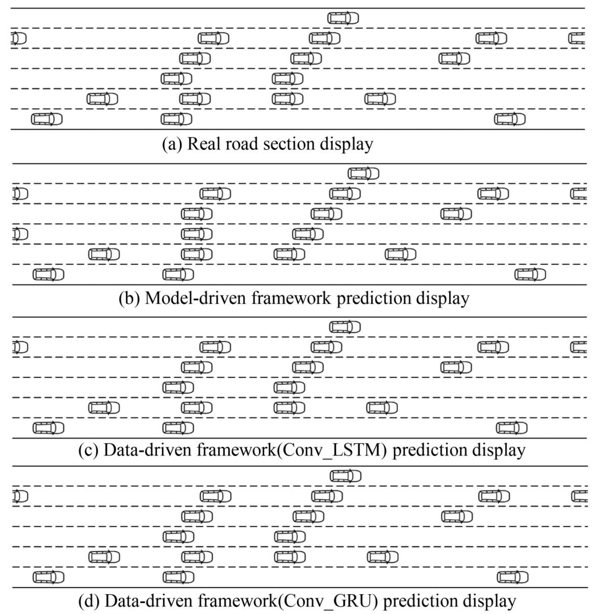
4.2. Prediction Display

Figure 3 shows the real road section and the road sections predicted by IDM, ConvLSTM, and ConvGRU. It can be seen that there is still a significant difference between the case predicted by IDM and the real one. As for the cases predicted by ConvLSTM and ConvGRU, they are basically the same as the real one.

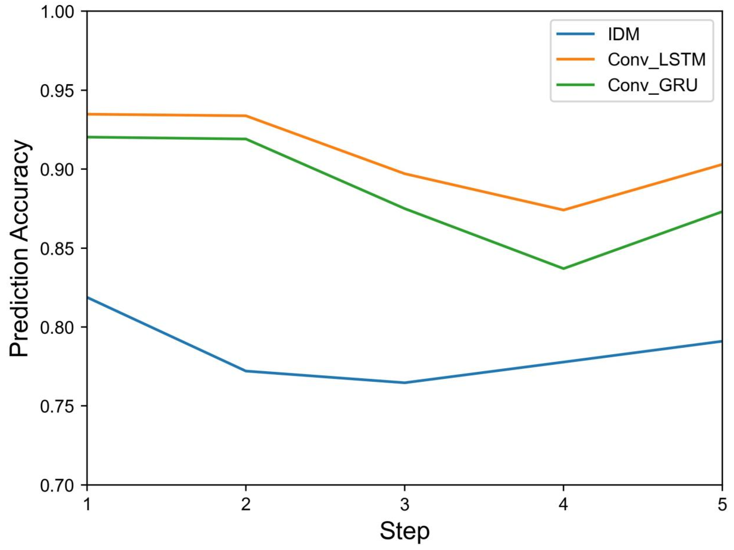
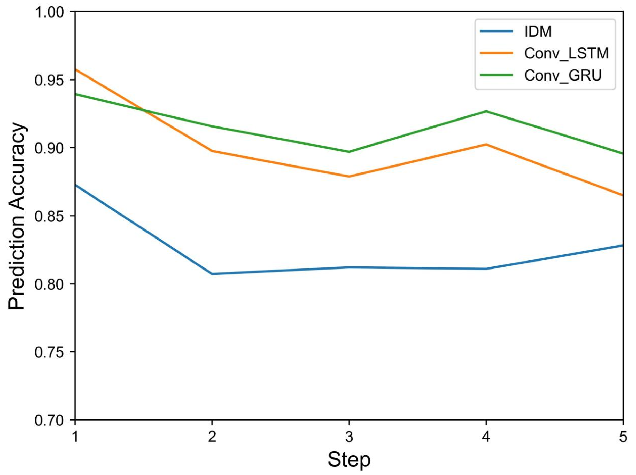
4.3. Continuous Prediction Comparison

To assess the framework’s performance in traffic simulation, continuous prediction capability was also tested on the test set, as depicted in Figure 4. The three curves, comprising continuous prediction results for ConvLSTM, ConvGRU, and IDM, clearly show that ConvLSTM and ConvGRU significantly outperform the IDM model in terms of prediction accuracy. It deserves recognition that continuous prediction using LSTM was omitted due to its relatively poor prediction performance. Additionally, ConvLSTM outperforms ConvGRU in the initial step but exhibits slightly lower performance in subsequent continuous predictions. Detailed results can be found in

Table 5. Continuous prediction comparison table.

Model	Step = 1	Step = 2	Step = 3	Step = 4	Step = 5
IDM	$87.27\%$	$80.72\%$	$81.21\%$	$81.10\%$	$82.82\%$
ConvLSTM	$95.76\%$	$89.76\%$	$87.88\%$	$90.24\%$	$86.50\%$
ConvGRU	$93.94\%$	$91.57\%$	$89.70\%$	$92.68\%$	$89.57\%$

.

4.4. Scalability Analysis

This section primarily focuses on comparing the scalability of large-scale simulation among the three aforementioned frameworks. In contrast to the trajectory prediction framework, where the input and output involve vehicle information, the simulation framework deals with road section data. This implies that in large-scale traffic flow simulations, the time complexity of the simulation framework is solely related to the overall road section size, and not dependent on the number of vehicles [45]. In other words, the time complexity for tracking vehicle trajectories is $O\left(n\right)$, while the time complexity for the simulation framework is a constant $O\left(1\right)$.

To assess the scalability of various frameworks, we conducted two sets of comparative experiments focused on computing time. One set involved controlling the simulation scale while varying the density, while the other set involved controlling the density while altering the simulation scale. The framework’s simulation inputs encompass scenes of varying sizes, while the inputs for the model-driven and trajectory prediction frameworks pertain to different vehicle quantities. The simulation results are presented in

Table 6. Different densities with the same simulation scale.

Scale	Density (pcu/(km × Lane))	Simulation Scale (Lane × Length)	Time Cost (s)
			ConvLSTM	ConvGRU	IDM	LSTM
Large	20	$6\times 1550$	1.6072	1.9766	0.4928	0.6621
	40	$6\times 1550$	1.6072	1.9766	0.9814	1.1221
	60	$6\times 1550$	1.6072	1.9766	1.4398	1.55544

and

Table 7. Different simulation scales with same density at 40 (pcu/(km × lane)).

Scale		Simulation Scale (Lane × Length)	Time Cost (s)
			ConvLSTM	ConvGRU	IDM	LSTM
Normal-scale	Small	$6\times 155$	1.1957	1.3621	0.1004	0.2718
	Middle	$6\times 775$	1.3595	1.5938	0.4928	0.6621
	Large	$6\times 1550$	1.6072	1.9766	0.9814	1.1221
Large-scale	Extra-Large	$6\times \mathrm{15,500}$	3.0077	8.6938	10.0700	9.9009
	Ultra-Large	$6\times \mathrm{155,000}$	45.4013	82.1890	145.9066	123.8712

. To ensure the experiment’s reliability, the scene size in each column of Table 6 corresponds precisely to the number of vehicles. It is significant to mention that the ’Large’ in the ’Scale’ column pertains to the simulation scale, a topic that is subsequently explored in greater detail in Table 7. The platform used for the simulation experiments is an Intel I5-10400F with 16 GB 2666 Mhz RAM and an NVIDIA GeForce GTX 1660 SUPER 6 GB.

From Table 6 and Table 7, we can find the following phenomena:

• The time cost of the data-driven framework remains unchanged with increasing density, in stark contrast to the other two frameworks, which show substantial variations. It should be emphasized that the time cost of the other two frameworks increases nearly linearly with density. Furthermore, the computational efficiency of the framework does not display a significant advantage over the other two frameworks when the scale is small or the density is low. However, in scenarios involving larger scale or higher density, its superiority becomes markedly evident.
• Regarding the results, as the size increases (from normal-scale to large), a noticeable phenomenon emerges: the time cost of the data-driven framework significantly rises. This can be attributed to the increase in DNN hidden layer parameters with the expanding size, leading to decreased computational efficiency. In contrast, for the other two frameworks, the results are similar, with computation time showing a near-linear relationship with size.
• Furthermore, in the case of large-scale scenes (extra-large and ultra-large), the computational efficiency of the data-driven framework surpasses that of the other two frameworks significantly. Notably, the linear growth observed in the normal-scale case is disrupted, mainly due to the substantial increase in computational load for the other two frameworks. However, the data-driven framework remains relatively insensitive to large-scale scenarios, and thus does not yield a significant improvement in computation time (It merits attention that for simulating the extra-large scene, we used SUMO software, and each simulation step took 7.149835 s).

In summary, it can be concluded that the data-driven framework exhibits distinct advantages for large-scale simulation when compared to the other two frameworks. Furthermore, the data-driven framework represents a potential enabler that has the potential to overcome existing limitations in the realm of large-scale simulation.

5. Transferability Analysis

To evaluate the generalizability and transferability of the data-driven framework, we utilized the framework model trained on the I-80 road segment within the NGSIM dataset. Subsequently, we applied this model to another road segment dataset, specifically US-101, and proceeded to compare the prediction results with those obtained using the IDM model.

As shown in

Table 8. Model transfer performance comparison.

Category	Model	Position Accuracy Rate
Model-driven traffic simulation	IDM+MOBIL	81.88%
Data-driven traffic simulation frame	ConvLSTM	93.48%
	ConvGRU	92.03%

and

Table 9. Continuous transfer prediction comparison table.

Model	Step = 1	Step = 2	Step = 3	Step = 4	Step = 5
IDM	81.88%	77.21%	76.47%	77.78%	79.10%
ConvLSTM	93.48%	93.38%	89.71%	87.41%	90.30%
ConvGRU	92.03%	91.91%	87.50%	83.70%	87.31%

, regardless of whether ConvLSTM or ConvGRU is employed as the deep neural network within the data-driven framework, the position prediction accuracy achieved on the US-101 dataset surpasses that of the IDM model. Although it may not reach the same prediction accuracy levels as observed on the I-80 dataset, it still demonstrates strong performance on the test set. Additionally, Figure 5 illustrates that both ConvLSTM and ConvGRU exhibit superior continuous prediction capabilities on the US-101 dataset compared to the IDM model.

6. Conclusions and Future Work

Traditional traffic simulation has predominantly depended on complex analytical models to mimic traffic behaviors accurately. This study, however, pivots towards a novel data-driven traffic simulation framework anchored in deep neural networks. By capitalizing on road section data, this framework adeptly models and forecasts the dynamics of road sections, facilitating a more nuanced traffic simulation. Central to our methodology are ConvLSTM and ConvGRU, serving as the primary models within this innovative framework. Their efficacy was tested using data from the I-80 road section, with their performance measured against traditional models such as IDM and LSTM trajectory prediction models. Additionally, the framework’s adaptability was evaluated through its application to the US-101 road section data. The salient findings from this study include the following:

• Demonstrating superior predictive accuracy, our data-driven framework significantly outperforms traditional models, achieving 97.22% accuracy in training and 95.76% in testing, a stark contrast to the 79.30% by model-driven frameworks. Despite its robust training set performance, the trajectory prediction aspect showed tendencies of overfitting, affecting test set accuracy.
• In evaluating continuous prediction capabilities, our framework consistently outstripped traditional models, even as accuracy naturally declined over five prediction steps. Notably, ConvLSTM showed particular prowess in single-step forecasts over ConvGRU, although it slightly lagged in multi-step predictions.
• An innovative loss function modification enhanced prediction accuracy by integrating tensor loss computation post-softmax operation into MSELoss, thus quickening network convergence and bolstering accuracy without succumbing to overfitting.
• Scalability analyses underscored the framework’s exceptional performance in large-scale simulations, despite not showing marked advantages in smaller setups. ConvLSTM, in particular, emerged as the superior choice for extensive simulation tasks over ConvGRU.
• Transferability tests affirmed the framework’s utility across different datasets, with a pre-trained model mirroring the original dataset’s accuracy at 93.48%.

Within the burgeoning field of automated and connected automated vehicles, the applications for this innovative data-driven framework are vast, offering a new horizon for vehicle communication and operational efficiency. At its foundation, the framework is powered by deep neural networks, highlighting the critical need for high-quality data to fully harness the framework’s predictive capabilities. It is imperative to recognize, however, that the reliance on the NGSIM dataset confines the scope of our study primarily to basic highway traffic modeling, rather than extending to more intricate traffic scenarios like signalized intersections or highway merge areas. For a truly holistic approach to traffic simulation that encompasses a variety of scenarios, further model development is indispensable. It is crucial to highlight that while the proposed framework exhibits significant advantages over traditional model-driven frameworks in terms of computational complexity and efficiency, it still encounters challenges such as memory overflow when dealing with ultra-large-scale simulations. In light of this, it becomes imperative to develop corresponding memory management optimization mechanisms based on this research to further enhance computational efficiency. This research represents a pioneering step towards a novel methodology in traffic flow simulation, suggesting substantial opportunities for future advancements. Integrating self-learning mechanisms into the model holds the promise of transforming it into a highly dynamic and adaptive tool for traffic management solutions, enabling the system to autonomously refine and optimize its predictive accuracy over time. Such advancements could significantly elevate the framework’s ability to anticipate and respond to complex traffic scenarios, thereby enhancing safety and efficiency on the road.

References

1. Ruan, T.; Wang, H.; Zhou, L.; Zhang, Y.; Dong, C.; Zuo, Z. Impacts of information flow topology on traffic dynamics of CAV-MV heterogeneous flow. IEEE Trans. Intell. Transp. Syst. 2022, 23, 20820–20835. [Google Scholar] [CrossRef]
2. Rajamani, R. Vehicle Dynamics and Control; Springer Science & Business Media: Berlin/Heidelberg, Germany, 2011. [Google Scholar]
3. Darbha, S.; Rajagopal, K. Intelligent cruise control systems and traffic flow stability. Transp. Res. Part C Emerg. Technol. 1999, 7, 329–352. [Google Scholar] [CrossRef]
4. Afrin, T.; Yodo, N. A probabilistic estimation of traffic congestion using Bayesian network. Measurement 2021, 174, 109051. [Google Scholar] [CrossRef]
5. Ruan, T.; Wang, H.; Jiang, R.; Li, X.; Xie, N.; Xie, X.; Hao, R.; Dong, C. A General Hierarchical Control System to Model ACC Systems: An Empirical Study. IEEE Trans. Intell. Transp. Syst. 2023, 25, 462–477. [Google Scholar] [CrossRef]
6. Han, G.; Han, Y.; Wang, H.; Ruan, T.; Li, C. Coordinated control of urban expressway integrating adjacent signalized intersections using adversarial network based reinforcement learning method. IEEE Trans. Intell. Transp. Syst. 2023, 25, 1857–1871. [Google Scholar] [CrossRef]
7. Hishikawa, T.; Iryo-Asano, M. Safety evaluation of personal mobility vehicles and pedestrians under mixed traffic flow using traffic simulation. Asian Transp. Stud. 2022, 8, 100049. [Google Scholar] [CrossRef]
8. Lucas, D.E.; Mirchandani, P.B.; Larry Head, K. Remote simulation to evaluate real-time traffic control strategies. Transp. Res. Rec. 2000, 1727, 95–100. [Google Scholar] [CrossRef]
9. Krajzewicz, D. Traffic simulation with SUMO—Simulation of urban mobility. In Fundamentals of Traffic Simulation; Springer: New York, NY, USA, 2010; pp. 269–293. [Google Scholar]
10. Tarko, A.P. Estimating the expected number of crashes with traffic conflicts and the Lomax Distribution—A theoretical and numerical exploration. Accid. Anal. Prev. 2018, 113, 63–73. [Google Scholar] [CrossRef] [PubMed]
11. Han, G.; Liu, X.; Wang, H.; Dong, C.; Han, Y. An Attention Reinforcement Learning–Based Strategy for Large-Scale Adaptive Traffic Signal Control System. J. Transp. Eng. Part A Syst. 2024, 150, 04024001. [Google Scholar] [CrossRef]
12. Ansariyar, A.; Taherpour, A. Investigating the accuracy rate of vehicle-vehicle conflicts by LIDAR technology and microsimulation in VISSIM and AIMSUN. Adv. Transp. Stud. 2023, 61, 37–52. [Google Scholar]
13. Xu, D.; Chen, Y.; Ivanovic, B.; Pavone, M. BITS: Bi-level imitation for traffic simulation. In Proceedings of the 2023 IEEE International Conference on Robotics and Automation (ICRA), London, UK, 29 May–2 July 2023; pp. 2929–2936. [Google Scholar]
14. Purnawan; Alfathira, R. Development of Traffic Delay and Queue Metamodel on Landslide Zone Based on Simulation Using VISSIM. In IOP Conference Series: Earth and Environmental Science; IOP Publishing: Bristol, UK, 2023; Volume 1173, p. 012050. [Google Scholar]
15. Ruan, T.; Zhou, L.; Wang, H. Stability of heterogeneous traffic considering impacts of platoon management with multiple time delays. Phys. A Stat. Mech. Its Appl. 2021, 583, 126294. [Google Scholar] [CrossRef]
16. Park, B.; Schneeberger, J. Microscopic simulation model calibration and validation: Case study of VISSIM simulation model for a coordinated actuated signal system. Transp. Res. Rec. 2003, 1856, 185–192. [Google Scholar] [CrossRef]
17. Wágner, T.; Ormándi, T.; Tettamanti, T.; Varga, I. SPaT/MAP V2X communication between traffic light and vehicles and a realization with digital twin. Comput. Electr. Eng. 2023, 106, 108560. [Google Scholar] [CrossRef]
18. Mądziel, M. Vehicle Emission Models and Traffic Simulators: A Review. Energies 2023, 16, 3941. [Google Scholar] [CrossRef]
19. Kotusevski, G.; Hawick, K. A Review of Traffic Simulation Software. 2009. Available online: https://api.semanticscholar.org/CorpusID:29284779 (accessed on 8 January 2024).
20. Luo, X.; Ge, Y.; Qu, W. The association between the Big Five personality traits and driving behaviors: A systematic review and meta-analysis. Accid. Anal. Prev. 2023, 183, 106968. [Google Scholar] [CrossRef] [PubMed]
21. AbuAli, N.; Abou-Zeid, H. Driver behavior modeling: Developments and future directions. Int. J. Veh. Technol. 2016, 2016, 6952791. [Google Scholar] [CrossRef]
22. Miyajima, C.; Takeda, K. Driver-behavior modeling using on-road driving data: A new application for behavior signal processing. IEEE Signal Process. Mag. 2016, 33, 14–21. [Google Scholar] [CrossRef]
23. Wastavino, L.; Toledo, B.; Rogan, J.; Zarama, R.; Muñoz, V.; Valdivia, J. Modeling traffic on crossroads. Phys. A Stat. Mech. Its Appl. 2007, 381, 411–419. [Google Scholar] [CrossRef]
24. Toledo, T.; Koutsopoulos, H.N.; Ben-Akiva, M. Integrated driving behavior modeling. Transp. Res. Part C Emerg. Technol. 2007, 15, 96–112. [Google Scholar] [CrossRef]
25. Ma, C.; Li, D. A review of vehicle lane change research. Phys. A Stat. Mech. Its Appl. 2023, 626, 129060. [Google Scholar] [CrossRef]
26. Geng, M.; Li, J.; Xia, Y.; Chen, X.M. A physics-informed Transformer model for vehicle trajectory prediction on highways. Transp. Res. Part C Emerg. Technol. 2023, 154, 104272. [Google Scholar] [CrossRef]
27. Aung, N.; Dhelim, S.; Chen, L.; Lakas, A.; Zhang, W.; Ning, H.; Chaib, S.; Kechadi, M.T. VeSoNet: Traffic-Aware Content Caching for Vehicular Social Networks Using Deep Reinforcement Learning. IEEE Trans. Intell. Transp. Syst. 2023, 24, 8638–8649. [Google Scholar] [CrossRef]
28. Tomar, R.S.; Verma, S.; Tomar, G.S. Prediction of lane change trajectories through neural network. In Proceedings of the 2010 International Conference on Computational Intelligence and Communication Networks, Liverpool, UK, 28–30 July 2010; pp. 249–253. [Google Scholar]
29. Cui, H.; Radosavljevic, V.; Chou, F.C.; Lin, T.H.; Nguyen, T.; Huang, T.K.; Schneider, J.; Djuric, N. Multimodal trajectory predictions for autonomous driving using deep convolutional networks. In Proceedings of the 2019 International Conference on Robotics and Automation (ICRA), Montreal, QC, Canada, 20–24 May 2019; pp. 2090–2096. [Google Scholar]
30. Zhang, X.; Sun, J.; Qi, X.; Sun, J. Simultaneous modeling of car-following and lane-changing behaviors using deep learning. Transp. Res. Part C Emerg. Technol. 2019, 104, 287–304. [Google Scholar] [CrossRef]
31. Li, X.Q.; Song, L.K.; Choy, Y.S.; Bai, G.C. Multivariate ensembles-based hierarchical linkage strategy for system reliability evaluation of aeroengine cooling blades. Aerosp. Sci. Technol. 2023, 138, 108325. [Google Scholar] [CrossRef]
32. Abdelaty, H.; Al-Obaidi, A.; Mohamed, M.; Farag, H.E. Machine learning prediction models for battery-electric bus energy consumption in transit. Transp. Res. Part D Transp. Environ. 2021, 96, 102868. [Google Scholar] [CrossRef]
33. Toledo, T. Driving behaviour: Models and challenges. Transp. Rev. 2007, 27, 65–84. [Google Scholar] [CrossRef]
34. Hoogendoorn, S.; Hoogendoorn, R.G.; Daamen, W. Wiedemann revisited: New trajectory filtering technique and its implications for car-following modeling. Transp. Res. Rec. 2011, 2260, 152–162. [Google Scholar] [CrossRef]
35. Kesting, A.; Treiber, M.; Helbing, D. Enhanced intelligent driver model to access the impact of driving strategies on traffic capacity. Philos. Trans. R. Soc. A Math. Phys. Eng. Sci. 2010, 368, 4585–4605. [Google Scholar] [CrossRef]
36. Kesting, A.; Treiber, M.; Helbing, D. General Lane-Changing Model MOBIL for Car-Following Models. Transp. Res. Rec. 2007, 1999, 86–94. [Google Scholar] [CrossRef]
37. Hochreiter, S.; Schmidhuber, J. LSTM can solve hard long time lag problems. In Advances in Neural Information Processing Systems; MIT Press: Cambridge, MA, USA, 1996; Volume 9. [Google Scholar]
38. Zhang, H.; Nan, Z.; Yang, T.; Liu, Y.; Zheng, N. A driving behavior recognition model with bi-LSTM and multi-scale CNN. In Proceedings of the 2020 IEEE Intelligent Vehicles Symposium (IV), Las Vegas, NV, USA, 19 October–13 November 2020; pp. 284–289. [Google Scholar]
39. Huang, X.; Sun, J.; Sun, J. A car-following model considering asymmetric driving behavior based on long short-term memory neural networks. Transp. Res. Part C Emerg. Technol. 2018, 95, 346–362. [Google Scholar] [CrossRef]
40. Shi, X.; Chen, Z.; Wang, H.; Yeung, D.Y.; Wong, W.K.; Woo, W.C. Convolutional LSTM network: A machine learning approach for precipitation nowcasting. In Advances in Neural Information Processing Systems; MIT Press: Cambridge, MA, USA, 2015; Volume 28. [Google Scholar]
41. Medel, J.R. Anomaly Detection Using Predictive Convolutional Long Short-Term Memory Units; Rochester Institute of Technology: Rochester, NY, USA, 2016. [Google Scholar]
42. Fu, R.; Zhang, Z.; Li, L. Using LSTM and GRU neural network methods for traffic flow prediction. In Proceedings of the 2016 31st Youth Academic Annual Conference of Chinese Association of Automation (YAC), Wuhan, China, 11–13 November 2016; pp. 324–328. [Google Scholar]
43. Irie, K.; Tüske, Z.; Alkhouli, T.; Schlüter, R.; Ney, H. LSTM, GRU, highway and a bit of attention: An empirical overview for language modeling in speech recognition. In Proceedings of the 17th Interspeech 2016, San Francisco, CA, USA, 8–12 September 2016; pp. 3519–3523. [Google Scholar]
44. Montanino, M.; Punzo, V. Trajectory data reconstruction and simulation-based validation against macroscopic traffic patterns. Transp. Res. Part B Methodol. 2015, 80, 82–106. [Google Scholar] [CrossRef]
45. Arora, S.; Barak, B. Computational Complexity: A Modern Approach. In Computational Complexity: A Modern Approach; Cambridge University Press: Cambridge, UK, 2009. [Google Scholar] [CrossRef]
Figure 1. Structure of the data-driven traffic simulation framework.
Sustainability 16 02666 g001
Figure 2. Diagram of error examples.
Sustainability 16 02666 g002
Figure 3. Prediction figures of road section with different models.
Sustainability 16 02666 g003
Figure 4. Continuous prediction accuracy rate line chart.
Sustainability 16 02666 g004
Figure 5. Continuous transfer prediction accuracy rate line chart.
Sustainability 16 02666 g005