TCN-Informer-Based Flight Trajectory Prediction for Aircraft in the Approach Phase

Abstract

Trajectory prediction (TP) is a vital operation in air traffic control systems for flight monitoring and tracking. The approach phase of general aviation (GA) aircraft is more of a visual approach, which is related to the safety of the flight and whether to go around. Therefore, it is important to accurately predict the flight trajectory of the approach phase. Based on the historical flight trajectories of GA aircraft, a TP model is proposed with deep learning after feature extraction in this study, and the hybrid model combines a time convolution network and an improved transformer model. First, feature extraction of the spatiotemporal dimension is performed on the preprocessed flight data by using TCN; then, the extracted features are executed by adopting the Informer model for TP. The performance of the novel architecture is verified by experiments based on real flight trajectory data. The results show that the proposed TCN-Informer architecture performs better according to various evaluation metrics, which means that the prediction accuracies of the hybrid model are better than those of the typical prediction models widely used today. Moreover, it has been verified that the proposed method can provide valuable suggestions for decision-making regarding whether to go around during the approach.

1. Introduction

General aviation (GA) encompasses a wide range of noncommercial and private aircraft operations that play a vital role in the transportation, educational training, and service industries. GA aircraft include light aircraft, helicopters, and gliders that operate in a variety of conditions and flight profiles, often involving flights to airports without complex air traffic control (ATC). ATC considers the trajectory of the aircraft at all stages of flight and manages these trajectories to avoid conflicts. However, the activities of GA aircraft in low-altitude airspace have increased in recent years. The flight environment in the air has become more complex and prone to aviation accidents, even under ATC [1]. Fatal accidents of aircraft are caused by various factors such as loss of control (LOC) [2,3], effects of wake vortices [4], related weather factors [5], and loss of situational awareness. To reduce the accident rate, ATC can be effectively improved by monitoring aircraft route deviation and detecting and handling route conflicts to optimize flight trajectories. Accurate trajectory prediction (TP) is indispensable for these methods.

Currently, different phases, such as the cruise phase and the approach phase, are predicted in flight trajectory prediction. However, different from the cruise phase, which can be autopiloted, the approach phase is mostly visual and approach-oriented and requires manual operation. Thus, the accident rate in the approach phase is higher than that in the other phases. In addition, the aircraft interrupts the approach when it does not have proper landing conditions and then requires a go-around. Focusing on the quality of go-around is an important step in ensuring flight safety and can prevent many unsafe events, but unnecessary go-around needs to be avoided. Go-around generates additional fuel consumption, which is not conducive to the recent proposal of energy savings and emission reduction. Therefore, flight trajectory prediction during the approach phase is critically linked to whether the airplane needs a go-around.

The TP of aircraft is the process of estimating the future position, speed, and altitude of aircraft based on historical flight data and various predictive models. However, the recent TP studies predominantly focus on commercial airline transportation for medium and large civil aircraft [6,7]. There are fewer studies on TP for GA aircraft. These aircraft typically operate under visual flight rules (VFR) or instrument flight rules (IFR). In general, the flight trajectory of a GA aircraft is more susceptible to various factors, including air traffic control directives, weather conditions [4], aircraft performance capabilities and navigational aids available [2,3], and the pilot’s own factors [8]. To accurately predict flight trajectory, a four-dimensional (4D)-TP enables more accurate and flexible route planning, including its position and altitude at specific points in time, to optimize flight trajectory, enhance safety, and improve airspace efficiency.

Existing TP methods can be categorized as state-space model methods and data-driven methods. For the state-space model methods [9,10,11,12] combined with flight environmental constraints, the flight trajectory is predicted by modeling the trajectory of the vehicle in the case of relative motion with air. For the data-driven approach [13,14,15,16,17,18], the data are organized to form information based on the large amount of collected flight trajectory data. This information is integrated and refined, and after training and fitting, a network architecture is formed. The flight trajectory can be regarded as multidimensional time series data. Therefore, the prediction method needs to be flexible and adaptable to the spatiotemporal characteristics of the aircraft. In this study, a data-driven approach based on a hybrid machine learning model is proposed to improve the performance of the TP task.

In our study, considering the large size of the time-series data of the flight parameters, a novel TP model was developed by extracting the spatiotemporal features of the sequential flight trajectory data and by exploring the network architecture for long sequence forecasting. The proposed TP architecture was performed for real GA aircraft under the approach phase with three training subjects, and the collected flight trajectory data were the Automatic Dependent Surveillance-Broadcast (ADS-B) data recorded by onboard equipment. In summary, the main contributions of our study are as follows:

• A temporal convolutional network (TCN)-Informer architecture is proposed for the TP of GA aircraft belonging to medium and long time series data. The dimension is incorporated as three spatial dimensions (latitude, longitude, and altitude). Recording and representing flight trajectory enables the analysis and reconstruction of flight trajectory in a more detailed and accurate manner. It also allows full visualization of the aircraft’s position and flight trajectory.
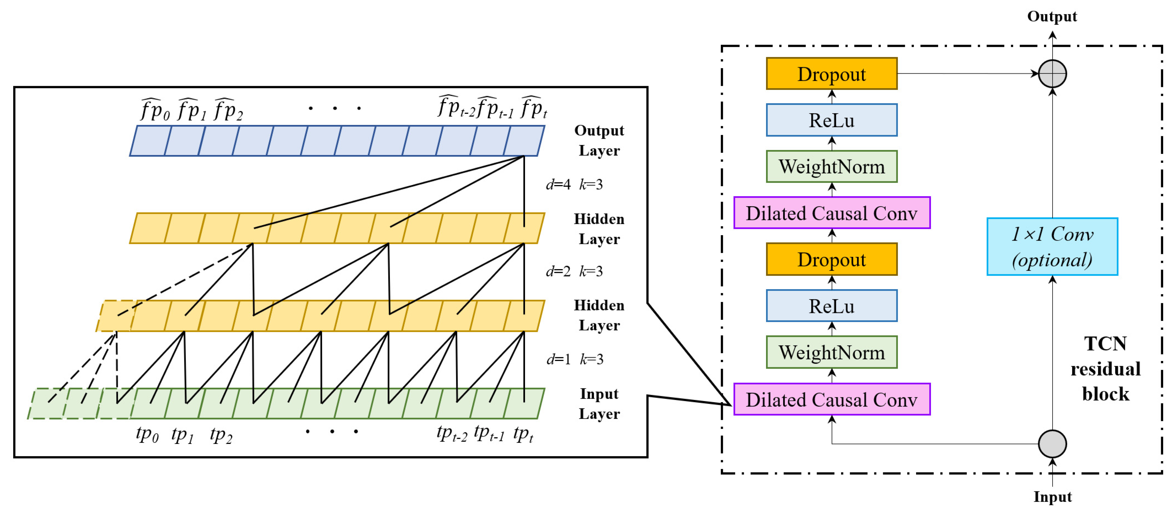
• The TCN model is used to extract the spatiotemporal features and trends of the long-term sequence of flight trajectory data. The TCN can keep the gradient stable and receive inputs of arbitrary length. The incorporated dilated causal convolutions can better change the receptive field size and better control the memory size of the model.
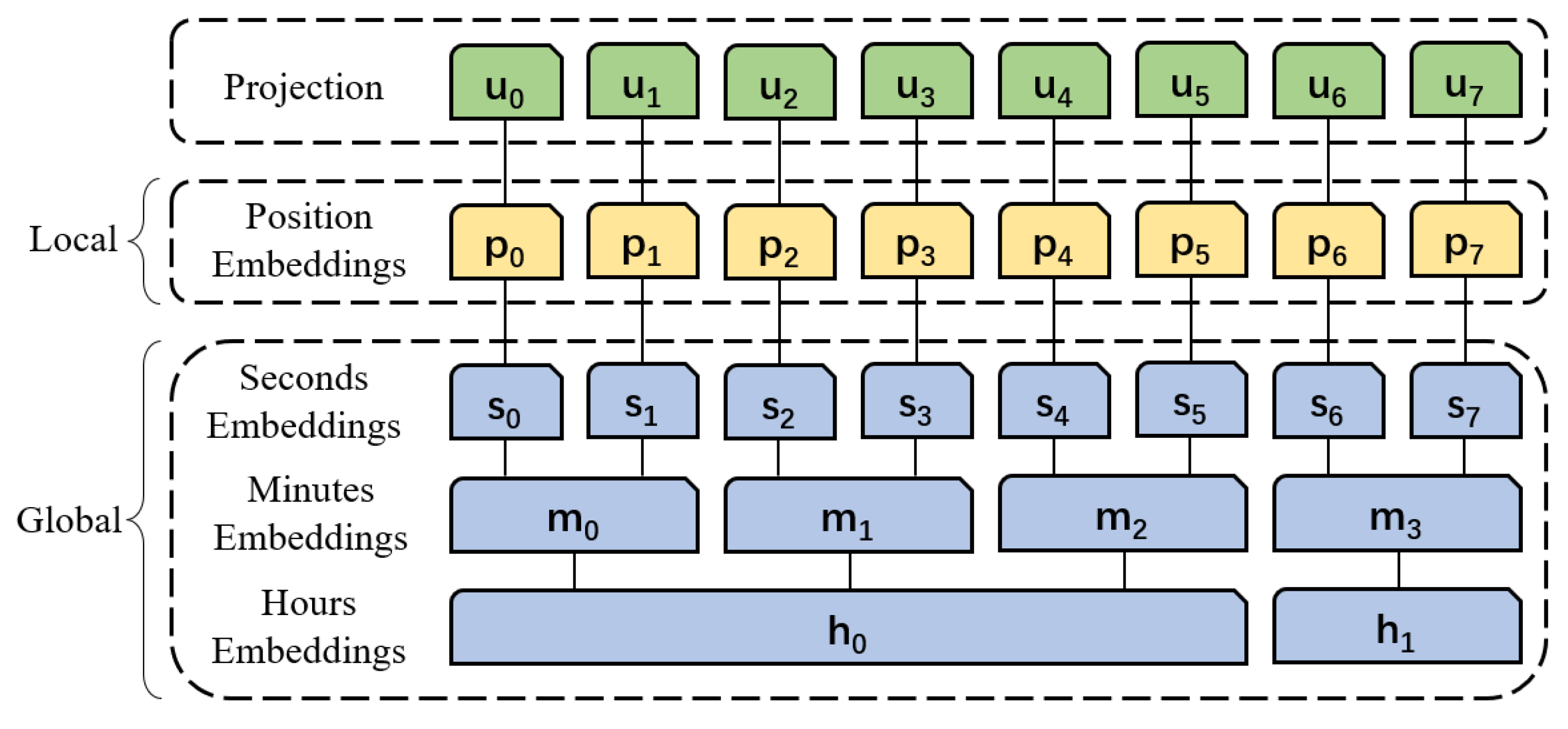
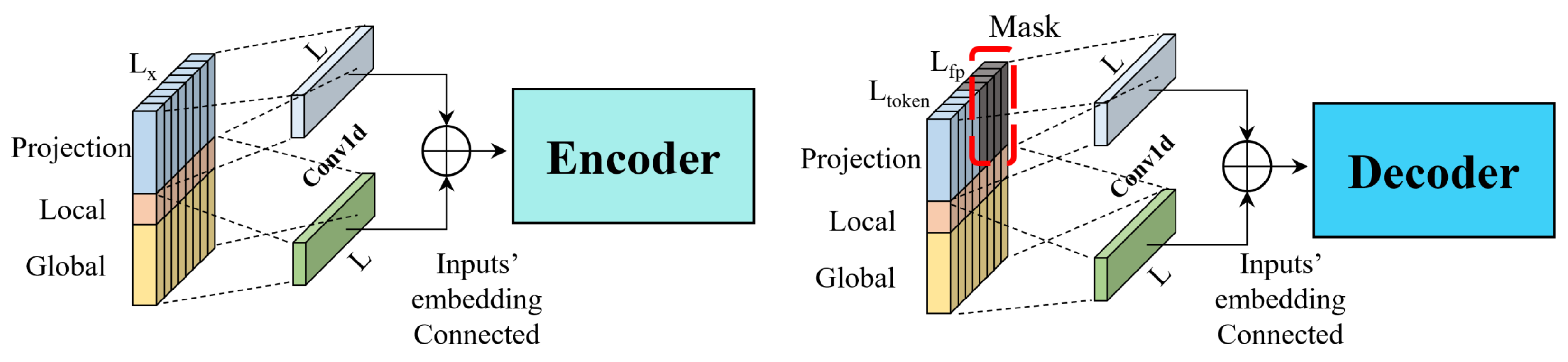
• Adaptive input embedding in the proposed TP model can take full advantage of the correlation in the time dimension. The integration of the Prob-Sparse self-attention mechanism and the distilling mechanism in the encoder-decoder architecture is superior to the data-driven method.
• By using real flight trajectory data from a variety of time-series network model comparison algorithm validations, the results show that the TCN-Informer architecture has the lowest prediction error in each dimension of the indicators and comprehensive evaluation indicators. The TCN-Informer architecture has high prediction accuracy in time-series prediction. Therefore, the prediction results can be used to identify standard flight trajectory gaps and to provide some assistance in deciding whether the airplane requires a go-around.

The remainder of this study is organized as follows: In Section 2, we review the current methods of the TP. The general architecture and details of our proposed model are given in Section 3. In Section 4, we describe the experimental setup, results analysis, and discussion. Section 5 provides the concluding remarks and future research.

2. Literature Review

Despite some fluctuations, the GA aircraft industry has shown resilience and potential for growth. Avionics and aircraft technology have seen significant advancements, making aircraft safer, more efficient, and easier to operate. Digital flight instruments, advanced navigation systems, and electronic flight bags have become more prevalent. The development of light aircraft and sport aircraft has gained traction, providing cost-effective and accessible options for aviation enthusiasts. Regulatory frameworks have evolved to address safety, security, and operational requirements for GA aircraft. Regulators and industry organizations collaborate to develop safety plans and measures to reduce accidents and incidents. The TP of the GA aircraft based on historical flight data are needed.

The TP methodologies for medium and large aircraft are not directly applicable to GA. Obtaining accurate and comprehensive historical flight trajectory data for training the TP models of GA aircraft is a challenging task. Unlike commercial aviation, where data are readily available from airlines, the flight trajectory data of GA aircraft is often scattered and incomplete. In addition, ensuring the quality and consistency of the collected data are critical for reliable predictions. Conducting the TP of the GA aircraft is conducive to safe operation and provides some assurance for sustainable development. Through in-depth analysis of various models, TP methods can be categorized into state estimation methods and data-driven methods.

2.1. State-Space Model Methods

Jiang [9] established a 4D-TP mathematical-physical model combined with an air-craft performance model and a control intent model, which integrated multiple types of information, such as weather, control intent, and aircraft performance. Obajemu [10] proposed an efficient four-dimensional trajectory generation method based on a high-fidelity aircraft model and a gain scheduling control strategy to optimize aircraft performance models. Salahudden [11] proposed a new method to generate an optimal climb trajectory with a standard stabilized climb equation that produced a unique combination of flight speed and track angle at each altitude to ensure a minimum fuel consumption and time-efficient climb. Yuan [12] developed a nonlinear dynamics model of a deformed vehicle and used recursive damped least squares to estimate and optimize the aircraft system model.

Although these methods allow changing the dynamic parameters of the state-space model itself, forming the dynamic system of the state-space model and efficiently dealing with missing data are more sensitive to the noise of the observations and prone to error accumulation during the prediction process, which affects the prediction results.

2.2. Data-Driven Methods

Data-driven methods organize a large amount of historical flight trajectory data to represent trajectory information, and the trained model based on the data are used for prediction. To solve the problem of extracting spatiotemporal features from trajectory data, Ma [13] proposed a novel hybrid architecture for 4D-TP based on the combination of a convolutional neural network (CNN) and long short-term memory (LSTM). Based on the dynamics of an airplane, Shi [14] proposed a constrained long-short-term memory network for the TP with three constraints for the climb, cruise, and descent/approach phases. Guo [15] presented FlightBERT, a novel architecture based on binary encoding representations that was capable of treating a TP task as a multi-binary classification problem. However, it is difficult to apply this method directly to actual scenes. Jia [16] proposed an attention-LSTM architecture to improve TP accuracy. To efficiently mine the flight trajectory information in the terminal area and grasp the spatial distribution characteristics of the adjacent traffic flow in the terminal area, a flight trajectory feature extraction model based on data attribute correlation was established, and the k-means were improved [17]. Aiming at the problems of insufficient feature utilization and unbalanced overall prediction results in machine learning 4D-TP, Zhao [18] proposed a fractal dimension feature prediction model based on quick access recorder (QAR) trajectory data.

Currently, data-driven approaches often rely on high-dimensional and large-scale data. Data-driven approaches typically require large amounts of labeled data to train the model. A larger amount of data correlates to a stronger model’s learning ability and a better training effect. However, in practical applications, there are problems such as overfitting on training data or low predictive accuracy in real-world flight parameter data. Therefore, in this study, a hybrid TCN-Informer architecture-based flight TP for GA aircraft is proposed. The overfitting problem can be effectively avoided by the TCN when extracting the flight parameter data. The unlabeled flight parameter data after the extraction of features can be used by the Informer model to train the network model. Therefore, in this study, the proposed model has some research value in solving the current problems of data-driven methods.

3. Methodology

3.1. Problem Formulation

The flight trajectory data consists of the status information of the entire flight process of the GA aircraft. The track points are presented as discrete data points. Each data point represents a specific position of the aircraft at a given time. The flight trajectory usually includes information such as the aircraft’s position, speed, heading, vertical speed, and other flight parameters [15]. The information for the flight trajectory used in this study is represented by Equation (1).

$$\mathit{tp}\triangleq \left[\mathit{Lon},\mathit{Lat},\mathit{Alt},\mathit{V},\mathit{Tra}\right]$$

(1)

where $\mathit{tp}$ denotes the vehicle track point and $\mathit{Lon},\mathit{Lat},\mathit{Alt}$ are the longitude, latitude, and altitude of the aircraft in three dimensions, respectively. The actual values of altitude in this study are the query normal height (QNH). $\mathit{V}$ is the indicated airspeed of the aircraft, and $\mathit{Tra}$ is the heading angle.

The existing machine learning-based flight trajectory prediction is usually formulated as a regression problem. A sequence of historical flight trajectories is available as $\mathit{TP}=\left\{{tp}_1,{tp}_2,\cdots ,{tp}_t\right\}$. The proposed TP model $\mathit{I}\left(\cdot \right)$ is capable of mapping an existing flight trajectory state sequence of time length $\mathit{t}$ to a 3D position sequence of time length $\mathit{L}$. The predicted sequence of the TP model outputs is the flight trajectory state from moment $\mathit{t}+1$ to moment $\mathit{t}+\mathit{L}$, denoted as $\mathit{FP}=\left\{f{p}_{t+1},{fp}_{t+2},\cdots ,{fp}_{t+L}\right\}$. $\mathit{fp}=\left[\mathit{Lon},\mathit{Lat},\mathit{Alt}\right]$ denotes the predicted track points. The TP formula can be expressed as Equation (2).

$$\left[{\mathit{tp}}_1{, \mathit{tp}}_2 , \cdots {, \mathit{tp}}_{\mathit{t}}\right]\stackrel{\mathit{I}\left(\cdot \right)}{\to }\left[{\mathit{fp}}_{\mathit{t}+1}{, \mathit{fp}}_{\mathit{t}+2}, \cdots {, \mathit{fp}}_{\mathit{t}+\mathit{L}}\right]$$

(2)

3.2. TCN-Based Feature Extraction

Considering the sequential flight trajectory data, the task of TP can be transformed into predicting ${\mathit{fp}}_1{, \mathit{fp}}_2, \cdots {, \mathit{fp}}_{\mathit{t}}$ in terms of ${\mathit{tp}}_1{, \mathit{tp}}_2 , \cdots {, \mathit{tp}}_{\mathit{t}}$. Due to the sequential characteristics of the flight trajectories, features of the flight trajectory data need to be explored in the time-space dimension. CNN is essentially a feed-forward neural network with a deep architecture for solving classification or regression problems. Researchers have improved feature extraction by applying CNN to time series data [19,20]. Bai [21] proposed the TCN algorithm, which is a modified CNN algorithm that can be used to solve time series representations.

The TCN uses a 1D fully convolutional network (FCN) architecture to show that the network produces outputs of the same length as the inputs and uses $\mathit{causal} \mathit{convolutions}$, convolutions where the outputs at time $\mathit{t}$ are convolved only with elements from time $\mathit{t}$ and earlier in the previous layer [22]. The TCN can be expressed as Equation (3). The computational complexity of the TCN is $O\left(L^2\right)$.

$$\mathit{TCN}=1\mathrm{D}\mathit{FCN}+\mathit{causal} \mathit{convolutions}$$

(3)

Simple causal convolution is limited in dealing with sequential tasks, causing difficulty in capturing the correlations between the points in a long-term time series. Therefore, null convolution with the ability to expand the sensory field is used. For a 1D sequence of inputs $\mathit{tp}\in {\mathit{R}}^{\mathit{n}}$ and filters $\mathit{f}:\left\{1,2,\cdots ,k-1\right\}$, the formula for the dilated convolution operation $F$ on a sequence element $s$ is denoted as Equation (4).

$$F\left(s\right)=\left(\mathit{tp}{\ast }_{d}f\right)\left(s\right)={\displaystyle \sum _{i=0}^{k-1}f\left(i\right)\cdot {\mathit{tp}}_{s-d\cdot i}}$$

(4)

where $d$ is the dilation factor, which is used to control the size of the interval. $k$ is the filter size, indicating the number of convolutional kernels. $\mathit{s}-\mathit{d}\cdot \mathit{i}$ indicates the past direction and $\ast$ is the convolution operator. When $\mathit{d}=1$, the dilated convolution recedes to a regular convolution. The use of dilated causal convolution effectively extends the receptive domain of the CNN. The architecture of the dilated causal convolution is shown in the left border (Figure 1). The kernel size is set to 3 in this study. The depth of the causal convolution is 3. The convolution shows that the output at time $\mathit{t}$ is associated with the input points from time 0 to time $\mathit{t}$. Each hidden layer has the same length as the input layer, and zero-padding is used to ensure that the subsequent layers have the same length.

Figure 1. Architecture of the dilated causal convolution and TCN residual block (dilation factors d = 1, 2, 4, and kernel size k = 3).

To address the challenge of vanishing or exploding gradients in deep networks, TCN often employs residual connections. These connections allow the model to learn the residual function, making it easier to train a very deep TCN and facilitating the capture of long-term dependencies. A residual block is a neural network block consisting of residual connections. A single residual block has two layers of null causal convolution, weight normalization, ReLU activation, and dropout. Batch weight normalization is used as the convolution filter. The ReLU activation function is applied to introduce nonlinearity and enhance the model representation. Dropout prevents overfitting and improves the model’s computing speed. When there is a difference in the length of the input and output data, residual connections are used to train the deep network by using an additional 1 × 1 convolutional skip connection. Skipping the residual join allows the network to learn the residual function, providing easier optimization and reducing the problem of vanishing or exploding gradients. The residual block of the TCN is shown on the right border (Figure 1).

The amount of information received by the TCN can be changed by adjusting the null parameters [23]. The acceptance field formula for the TCN is expressed as Equation (5):

$${\mathit{R}}_{\mathit{field}}=1+\left(k+1\right)\times N_{\mathit{stack}}\times {\displaystyle \sum _{{}^i}{d}_i}$$

(5)

where $\mathit{R}$ denotes the receptive domain of the TCN, ${\mathit{N}}_{\mathit{stack}}$ denotes the number of stacks, and ${\mathit{d}}_{\mathit{i}}$ denotes the dilation factor of the $\mathit{i}$th layer.

3.3. Informer Based Sequence Prediction

Actually, the TP task in this work can be viewed as long sequence time series forecasting (LSTF), which requires a higher predictive ability of the model. To address the problem that hinders the extended predictive ability of LSTF, Zhou [24] designed an efficient LSTF model, i.e., the Informer model, which proposes the following improvements over the transformer model.

3.3.1. Adaptive Input Embedding

In addition to the local time-series information, sometimes hierarchical time-series information, such as specific hours, minutes, and seconds, is also needed. The Informer model uses adaptive input embedding to capture the features of the time series data [25]. The Informer model contains a three-level feature input representation (Figure 2).

Figure 2. Composition architecture of the Informer model input.

Three positional embedding representations are shown: local timestamps, global timestamps, and the alignment dimension. Positive cosine processing is used to ensure local context through fixed position embedding at each track point, as shown in Equations (6) and (7).

$$\mathit{PE}\left(\mathit{pos},2\mathit{j}\right)=\mathit{sin}\left(\mathit{pos}/{\left({2\mathit{L}}_{\mathit{tp}}\right)}^{2\mathit{j}/{\mathit{d}}_{\mathit{model}}}\right)$$

(6)

$$\mathit{PE}\left(\mathit{pos},2\mathit{j}+1\right)=\mathit{cos}\left(\mathit{pos}/{\left({2\mathit{L}}_{\mathit{tp}}\right)}^{2\mathit{j}/{\mathit{d}}_{\mathit{model}}}\right)$$

(7)

where ${\mathit{d}}_{\mathit{model}}$ denotes the feature dimension. ${\mathit{L}}_{\mathit{tp}}$ denotes the length of the input sequence. $\mathit{pos}$ denotes the position of the current input track point in the input track sequence, and $\mathit{j}\in \left\{1,\cdots ,d/2\right\}$.

The global timestamp is represented using the learnable stamp embedding ${\mathit{SE}}_{\left(\mathit{pos}\right)}$. A one-dimensional convolutional filter is used to map the scalar ${\mathit{tp}}_i^t$ to the d-dimensional vector $u_i^t$. The input representation vector for the combination of the three position embeddings is denoted as Equation (8).

$${\mathit{X}}_{\mathit{feed}\left[\mathit{i}\right]}^{\mathit{t}}{=\alpha \mathit{u}}_{\mathit{i}}^{\mathit{t}}{+\mathit{PE}}_{\left({\mathit{L}}_{\mathit{tp}}\times \left(\mathit{t}-1\right)+\mathit{i}\right)}+{{\displaystyle \sum _{\mathit{p}}\left[{\mathit{SE}}_{\left({\mathit{L}}_{\mathit{tp}}\times \left(\mathit{t}-1\right)+\mathit{i}\right)}\right]}}_{\mathit{p}}$$

(8)

where $\mathsf{\alpha }$ is the hyperparameter used to balance the high-dimensional mapping of the flight trajectory data with the location and timestamp high-dimensional mapping. If the data have been normalized, $\alpha =1$. $u$ denotes a one-dimensional convolution process to align the dimensions to align the vector dimensions, and $\mathit{i}\in \left\{1,\cdots {,\mathit{L}}_{\mathit{tp}}\right\}$.

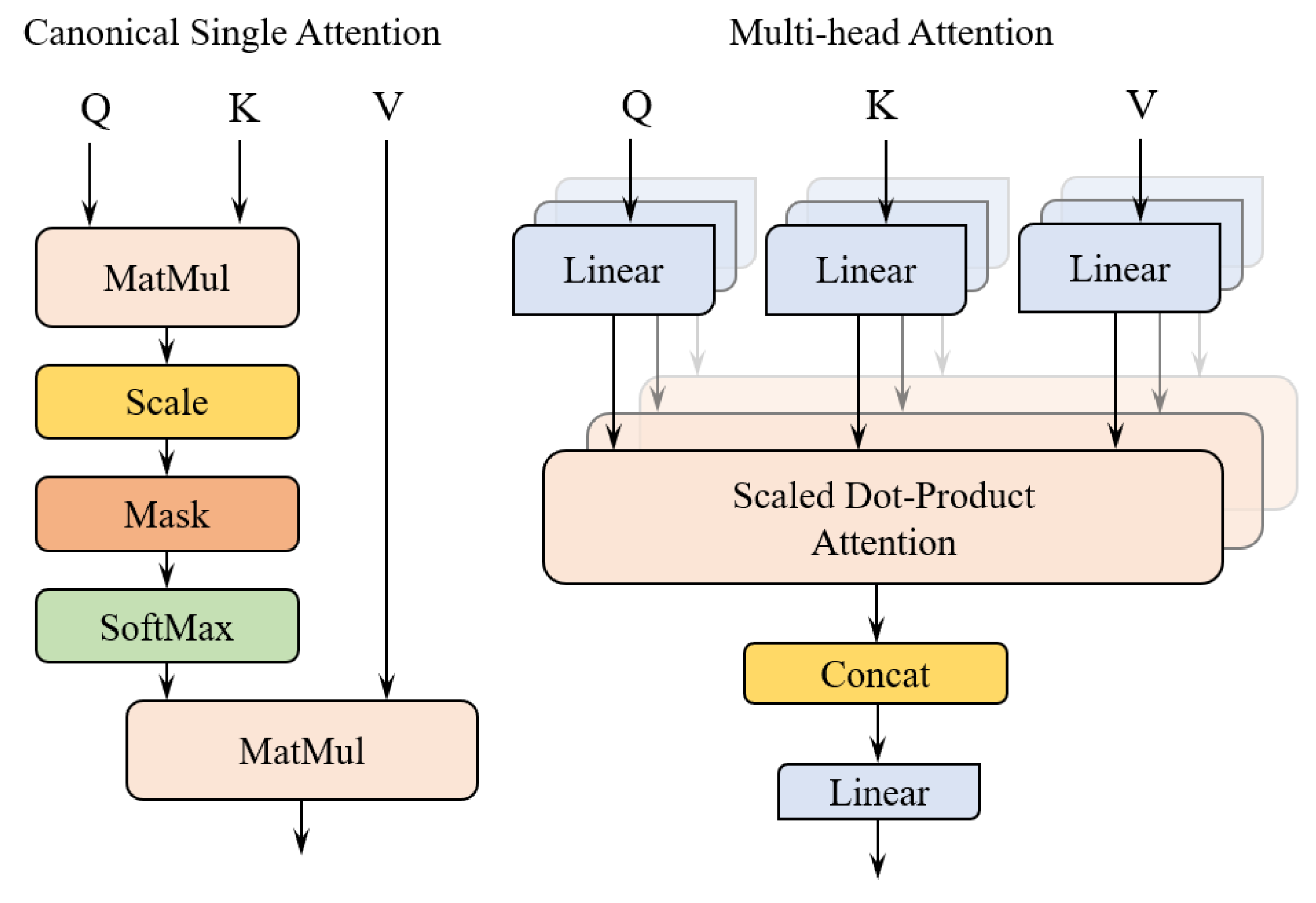
3.3.2. ProbSparse Self-Attention Mechanism

To improve the overall performance of the model in time series forecasting tasks, a ProbSparse self-attention mechanism is introduced in the Informer model to improve the computational efficiency of self-attention in a long time series setting. To capture the importance of different positions in the attention sequence, a probabilistic sparse mechanism is introduced to optimize the attention mechanism [26]. This method is particularly useful when dealing with long sequences or resource-constrained environments. Self-attention is based on the probability $\mathit{p}(\left.{\mathit{k}}_{\mathit{j}}\right|{\mathit{q}}_{\mathit{i}})$ and combined with Value values to obtain the output, which requires a total of ${\mathit{O}(\mathit{L}}_{\mathit{Q}}{\mathit{L}}_{\mathit{K}})$ memory usage for dot-product computation [27]. The informant uses the Kullback–Leibler (KL) divergence to assess the importance of attention. The formula for calculating KL divergence is expressed as Equation (9):

$$\mathit{KL}\left(\mathit{q}‖\mathit{p}\right)={\displaystyle \sum _{\mathit{j}=1}^{{\mathit{L}}_{\mathit{k}}}\frac{1}{{\mathit{L}}_{\mathit{K}}}\mathit{ln}\frac{\frac{1}{{\mathit{L}}_{\mathit{K}}}}{\frac{{\mathit{k}(\mathit{q}}_{\mathit{i}}{,\mathit{k}}_{\mathit{l}})}{{\displaystyle {\sum }_{\mathit{l}}{\mathit{k}(\mathit{q}}_{\mathit{i}}{,\mathit{k}}_{\mathit{l}})}}}}=\mathit{log}{\displaystyle \sum _{\mathit{j}=1}^{{\mathit{L}}_{\mathit{k}}}{\mathit{e}}^{\frac{{\mathit{q}}_{\mathit{i}}{\mathit{k}}_{\mathit{l}}^{\mathit{T}}}{\sqrt{\mathit{d}}}}}-\frac{1}{{\mathit{L}}_{\mathit{K}}}{\displaystyle \sum _{\mathit{j}=1}^{{\mathit{L}}_{\mathit{k}}}\frac{{\mathit{q}}_{\mathit{i}}{\mathit{k}}_{\mathit{j}}^{\mathit{T}}}{\sqrt{\mathit{d}}}}-{\mathit{lnL}}_{\mathit{K}}$$

(9)

where $p\left(k_j|q_i\right)$ is the probability of the i-th query’s attention for all keys. $q\left(k_j|q_i\right)=\frac{1}{L_K}$ is the uniform distribution. ${\mathit{L}}_{\mathit{K}}$ is the sequence length. ${\mathit{k}(\mathit{q}}_{\mathit{i}}{,\mathit{k}}_{\mathit{l}})$ is the intermediate value of the i-th query and the j-th key when performing the softmax activation function calculation. Dropping the constant ${\mathit{ln} \mathit{L}}_{\mathit{K}}$,The sparsity score metric of the i-th query is denoted by Equation (10).

$$\mathit{M}\left({\mathit{q}}_{\mathit{i}},\mathit{K}\right)=\mathit{log}{\displaystyle \sum _{\mathit{j}=1}^{{\mathit{L}}_{\mathit{k}}}{\mathit{e}}^{\frac{{\mathit{q}}_{\mathit{i}}{\mathit{k}}_{\mathit{l}}^{\mathit{T}}}{\sqrt{\mathit{d}}}}}-\frac{1}{{\mathit{L}}_{\mathit{K}}}{\displaystyle \sum _{\mathit{j}=1}^{{\mathit{L}}_{\mathit{k}}}\frac{{\mathit{q}}_{\mathit{i}}{\mathit{k}}_{\mathit{j}}^{\mathit{T}}}{\sqrt{\mathit{d}}}}$$

(10)

Based on the above measurement, by allowing each key to only focus on the $u$ dominant queries, the ProbSparse self-attention is denoted as Equation (11).

$$\mathit{Attention}\left(\mathit{Q},\mathit{K},\mathit{V}\right)=\mathit{softmax}\left(\frac{{\overline{\mathit{Q}}\mathit{K}}^{\mathit{T}}}{\sqrt{\mathit{d}}}\right)\mathit{V}$$

(11)

where $\mathit{Q},\mathit{K},\mathit{V}$ are three matrices of the same size obtained by linear transformation of the input eigenvariables. $\mathit{Q} ¯$ is obtained by probabilistic sparsification of $Q$, which contains only the Top-$u$ queries under the sparsity measure $\mathit{M}\left({\mathit{q}}_{\mathit{i}},\mathit{K}\right)$. In practice, the input lengths of queries and keys are typically equivalent in the self-attention computation, i.e., ${\mathit{L}}_{\mathit{Q}}={\mathit{L}}_{\mathit{K}}=\mathit{L}$, such that the total ProbSparse self-attention time complexity and space complexity are $\mathit{O}\left(\mathit{L} \mathit{lnL}\right)$. ProbSparse self-attention is used to solve the self-attention dot product computation with time complexity optimized from $O\left(L^2\right)$ to $\mathit{O}\left(\mathit{L} \mathit{lnL}\right)$.

ProbSparse self-attention can generate different queries with different sparsities for each header, avoiding the loss of important information. $n$-head self-attention in the same layer is denoted as Equations (12) and (13).

$$\mathit{Multihead}\left(\mathit{Q},\mathit{K},\mathit{V}\right)=\mathrm{Concat}\left({\mathit{head}}_1,\cdots ,{\mathit{head}}_{\mathit{n}}\right){\mathit{W}}^{\mathit{O}}$$

(12)

$${\mathit{head}}_{\mathit{i}}=\mathit{Attention}\left({\mathit{QW}}_{\mathit{i}}^{\mathit{Q}}{,\mathit{KW}}_{\mathit{i}}^{\mathit{K}}{,\mathit{VW}}_{\mathit{i}}^{\mathit{V}}\right)$$

(13)

where $\mathit{Concat}\left(\cdot \right)$ denotes the connection operation, $W^Q,W^K\in R^{d_{\mathit{model}}\times {\mathit{d}}_{\mathit{k}}}$, $W^V\in R^{d_{\mathit{model}}\times {\mathit{d}}_{\mathit{v}}}$, $W^O\in R^{d_{\mathit{model}}\times h{\mathit{d}}_{\mathit{v}}}$ and $d_k=d_v=d_{\mathit{model}}/h$. Multi-head attention sends $\mathit{Q},\mathit{K},\mathit{V}$ to the attention aggregation in parallel by projecting them n times using different learnable linear projections. The outputs of the h attention aggregations are then stitched together and transformed by another learnable linear projection to produce the final output. Self-attention also uses this projection method, which changes from single attention to multiple sides [28], named multi-head attention (Figure 3).

Figure 3. Canonical single-self-attention function and multi-head attention.

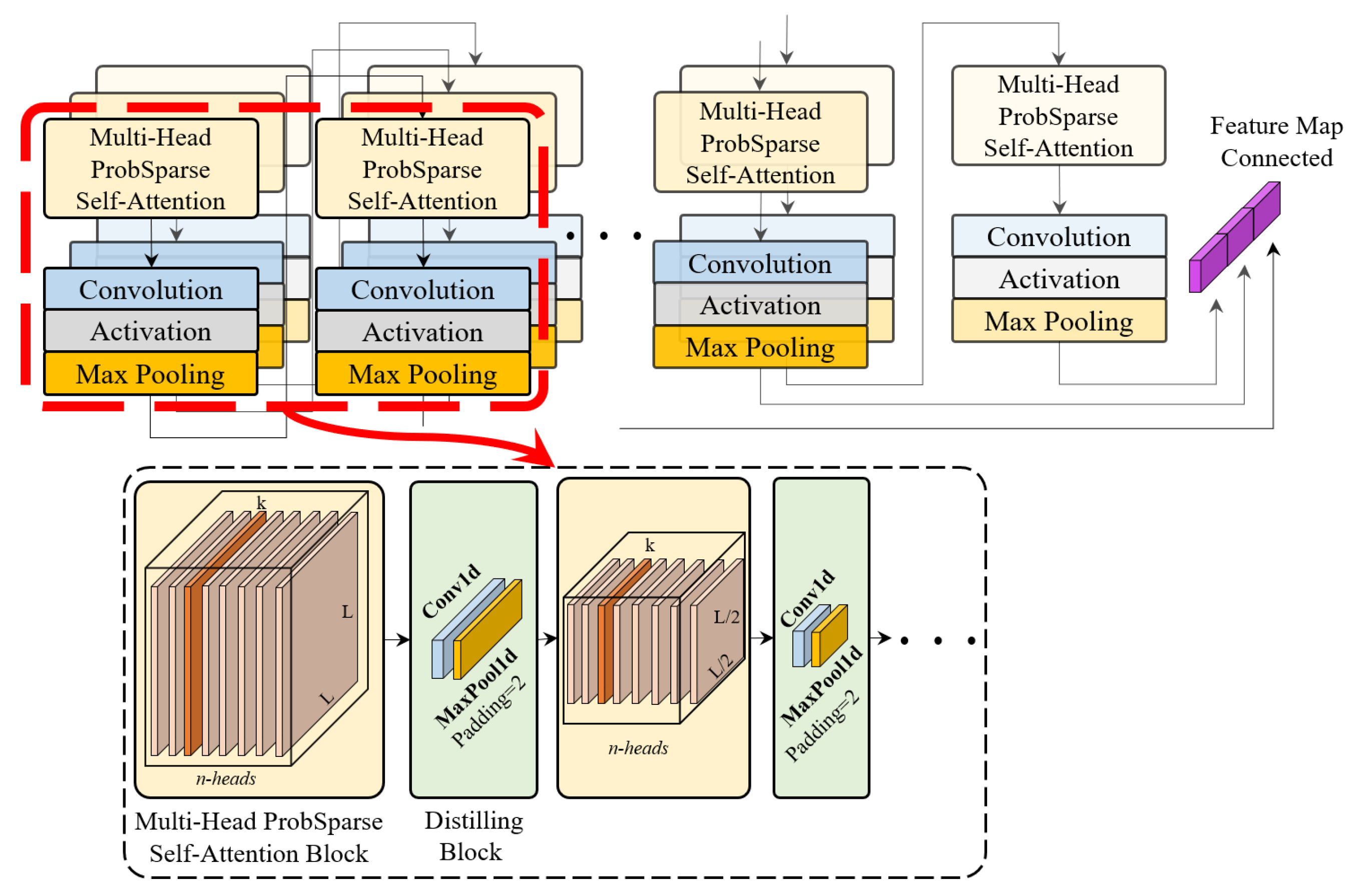
3.3.3. Distilling Mechanism

The distilling operation shortens the length of the input sequence of each layer to reduce the number of dimensions and network parameters. Attention is highlighted as a method to efficiently handle extremely long input sequences, reducing the memory usage of the stacked layers.

After probabilistic sparsification, the distilling operation enhances the dominant high-level features and generates a centralized self-attention feature map in the next layer, thus compressing the feature dimensions and highlighting the dominant features [28]. The distilling process from layer $j$ to layer $j+1$ is expressed as Equation (14):

$${\mathit{X}}_{\mathit{j}+1}^{\mathit{t}}=\mathit{MaxPool}\left(\mathit{ELU}\left(\mathit{Conv}1\mathit{d}\left({\left[{\mathit{X}}_{\mathit{j}}^{\mathit{t}}\right]}_{\mathit{AB}}\right)\right)\right)$$

(14)

where ${\left[\cdot \right]}_{AB}$ denotes the attention block and contains the basic operations in the attention block. The distilling method downsamples the features by adding convolutional pooling operations between the neighboring attention blocks. $\mathit{Conv}1\mathit{d}(·)$ denotes a 1-D convolutional filter with a kernel width of 3 and adds an ELU activation layer in the time dimension. When x ≥ 0, the function is able to mitigate gradient vanishing; when x < 0, the function is able to be more robust to input variations or noise. This activation function is shown in Equation (15). MaxPool represents the maximum pooling downsampling operation, with a pooling window size of 2. After each layer ${\mathit{X}}^{\mathit{t}}$ is downsampled to 1/2 of the original length. This process is able to reduce the overall memory usage to $\mathit{O}\left(\left(2-\epsilon \right)\mathit{LlogL}\right)$, as a way of compressing the features and reducing the number of parameters.

$$\mathit{ELU}\left(\mathit{x}\right)=\left\{\begin{array}{c}\mathit{x} , \mathit{if} \mathit{x}\ge 0\\ \mathsf{\alpha }\left({\mathit{e}}^{\mathit{x}}-1\right), \mathit{if} \mathit{x}<0\end{array}\right.$$

(15)

3.4. Hybrid Flight Trajectory Prediction Network

When dealing with sequences with time spans and multiple inputs and outputs, a sequence-to-sequence architecture is often used to enhance the linkage of time series for prediction. In this study, a hybrid TP method that combines the advantages of the TCN model and the Informer model is proposed as follows (Figure 4). The model reflects the entire process of TP, consisting of three parts: feature extraction of flight trajectory data, feature embedding, and the encoder and decoder of the trajectory prediction.

Figure 4. Architecture of the TCN-Informer.

3.4.1. Feature Extraction of the Trajectory Data

Considering the sequential flight trajectory data ${\mathit{tp}}_1{, \mathit{tp}}_2 , \cdots {, \mathit{tp}}_{\mathit{t}}$, the feature extraction for the historical flight trajectory consisting of the preprocessed trajectory points is executed by utilizing the TCN network. The TCN network often favors the processing of sequential data, and thus the TCN is not susceptible to gradient vanishing and explosion problems when dealing with TP tasks [29].

To exploit the TCN architecture, the cropping input tensor is first set to remove the extra padding. Then, the convolution operation is performed on the sequence data in the time dimension. To enhance model feature extraction, the residual network consists of multiple residual blocks connected in series, as shown in the TCN section circled in Figure 4. Each residual block is shown in Figure 1. The flight trajectory data begins to be processed through a convolutional layer with weight normalization. The input variable features of the aircraft’s spatial position, velocity, and trajectory angle variables can be efficiently extracted by a one-dimensional convolution. The next nonlinearity is introduced through the ReLU activation function to make the TCN model more than just an overly complex linear regression model. Finally, regularization is introduced by introducing dropout. The steps as above are repeated twice in the residual block before obtaining the output ${\mathit{x}}_1{, \mathit{x}}_2 , \cdots {, \mathit{x}}_{\mathit{t}}$. When the input and output widths differ, an additional 1 × 1 convolution is used to ensure that the same-shaped tensor is received. The output ${\mathit{x}}_1{, \mathit{x}}_2 , \cdots {, \mathit{x}}_{\mathit{t}}$ is brought into the Informer model for flight trajectory prediction.

3.4.2. Embedding of the Trajectory Data

The track points after performing feature extraction of the flight trajectory data are added to the embedding layer after masking. In a rolling prediction setup with a fixed window size, the main input to the Informer model is the normalized flight trajectory data ${\mathit{X}}^{\mathit{t}}=\left\{{\mathit{x}}_1^{\mathit{t}},\cdots {,\mathit{x}}_{{\mathit{L}}_{\mathit{x}}}^{\mathit{t}}{|\mathit{x}}_{\mathit{i}}^{\mathit{t}}\in {\mathit{R}}^{\mathit{dx}}\right\}$ from the previous $\mathit{t}$ moments, with five influence factors. ${\mathit{L}}_{\mathit{x}}$ denotes the length of the current input sequence, and each point in this sequence is a vector of $\mathit{dx}$ dimensions. The vector whose prediction corresponds to the output is ${\mathit{fp}}^{\mathit{t}}=\left\{{\mathit{fp}}_1^{\mathit{t}},\cdots {,\mathit{fp}}_{{\mathit{L}}_{\mathit{fp}}}^{\mathit{t}}{|\mathit{fp}}_{\mathit{i}}^{\mathit{t}}\in {\mathit{R}}^{\mathit{d} \mathit{fp}}\right\}$, with three influence factors. ${\mathit{L}}_{\mathit{fp}}$ denotes the length of the current output sequence, where each point, is an $\mathit{d} \mathit{fp}$-dimensional vector. The embedding layer deforms ${\mathit{X}}^{\mathit{t}}$ into a matrix ${\mathit{X}}_{\mathit{feed}\_\mathit{en}}^{\mathit{t}}\in {\mathit{R}}^{{\mathit{L}}_{\mathit{x}}\times {\mathit{d}}_{\mathit{model}}}$ by adaptive input embedding, as in Section 3.3.1. The deformation is introduced into the encoder.

The masked embedding layer deforms a matrix of long sequence fragments of length ${\mathit{L}}_{\mathit{token}}$ in ${\mathit{X}}^{\mathit{t}}$ combined with a 0 matrix of the same shape as the predicted target into the combined matrix ${\mathit{X}}_{\mathit{feed}\_\mathit{de}}^{\mathit{t}}$ as shown in Equation (16); the function of ${\mathit{X}}_{\mathrm{token}}^{\mathit{t}}\in R^{{\mathit{L}}_{\mathrm{token}}\times {\mathit{d}}_{\mathit{model}}}$ is the starting token and ${\mathit{X}}_0^{\mathit{t}}\in R^{{\mathit{L}}_{\mathrm{fp}}\times {\mathit{d}}_{\mathit{model}}}$ is a placeholder for the target sequence (with the scalar set to 0) as shown in the gray part (Figure 5). The deformed ${\mathit{X}}_{\mathit{feed}\_\mathit{de}}^{\mathit{t}}$ is introduced into the decoder.

$${\mathit{X}}_{\mathit{feed}\_\mathit{de}}^{\mathit{t}}=\mathrm{Concat}\left({\mathit{X}}_{\mathrm{token}}^{\mathit{t}},{\mathit{X}}_0^{\mathit{t}}\right)\in R^{\left({\mathit{L}}_{\mathrm{token}}+{\mathit{L}}_{\mathrm{fp}}\right)\times {\mathit{d}}_{\mathit{model}}}$$

(16)

Figure 5. Data embedding methods for the encoders and decoders.

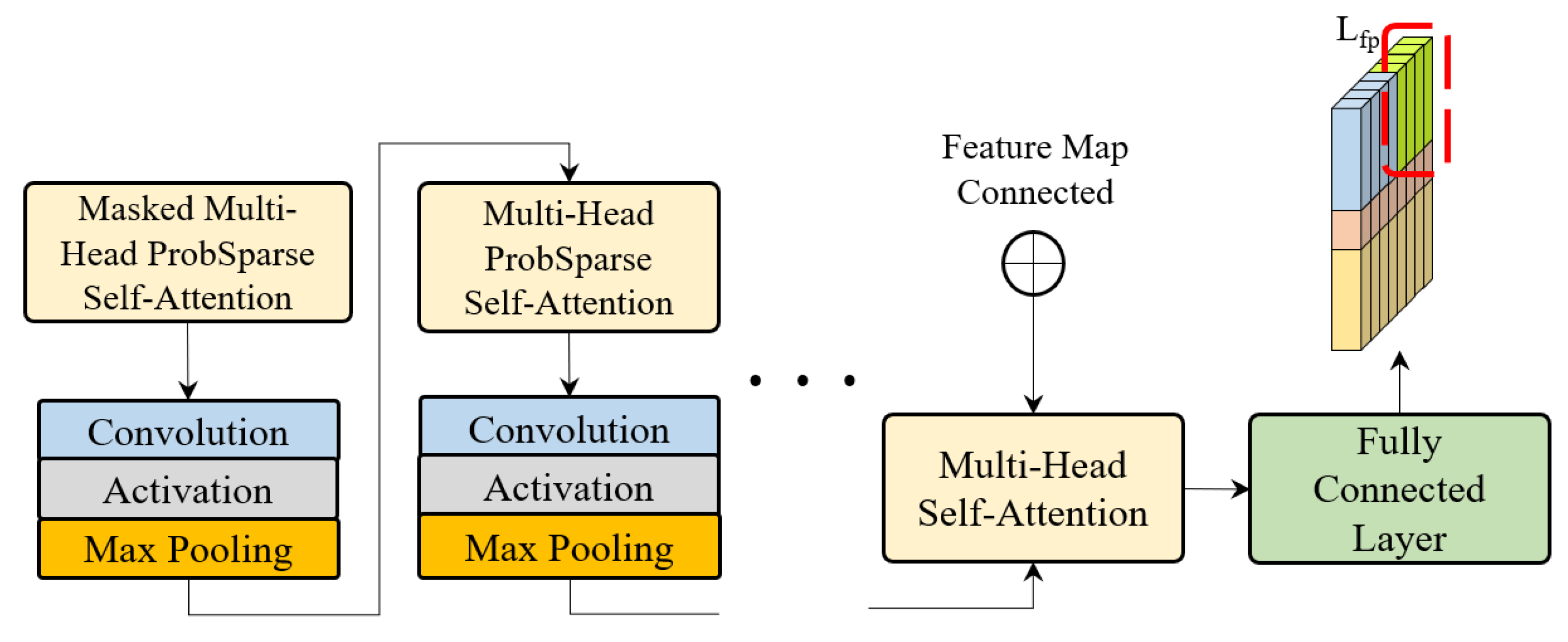
3.4.3. Encoder and Decoder of the TP model

The integrated Informer block internally consists of an encoder and a decoder. The encoder and the decoder accept data inputs, but the data inputs are different. The encoder encodes ${\mathit{X}}_{\mathit{feed}\_\mathit{en}}^{\mathit{t}}$ into ${\mathit{H}}^{\mathit{t}}=\left\{{\mathit{h}}_1^t,\cdots ,{\mathit{h}}_{{\mathit{L}}_{\mathit{h}}}^t\right\}$ and then the decoder decodes ${\mathit{H}}^{\mathit{t}}$ into the output ${\mathit{fp}}_{\mathit{k}+1}^{\mathit{t}}$. ${\mathit{X}}_{\mathit{feed}\_\mathit{en}}^{\mathit{t}}$ is the input of the encoder, and the feature map connection is output after several operations in the multi-head ProbSparse self-attention block and the distilling block. The architecture of the encoder is shown in Figure 6. To enhance the robustness of extracting long sequence inputs and to prevent excessive loss of information, ${\mathit{X}}_{\mathit{feed}\_\mathit{en}}^{\mathit{t}}$ is sliced according to the time dimension. The length of the input sequence of ${\mathrm{x}}_{\mathrm{i}}^{\mathrm{t}}\in {\mathrm{R}}^{{\mathit{L}}_{\left(\mathit{i}\right)}\times {\mathit{d}}_{\mathit{model}}}$ is $\mathit{L}\left(\mathit{i}\right)={\mathrm{L}}_{\mathrm{x}}/2^{\left(\mathit{i}-1\right)},\mathit{i}\in \left\{1,2,\cdots \right\}$. Each slice ensures the alignment of the output dimension by removing one operation of the multi-head ProbSparse self-attention block and the distilling mechanism block. Then, all feature maps are connected.

Figure 6. Architecture of the encoder part.

The ${\mathit{X}}_{\mathit{feed}\_\mathit{de}}^{\mathit{t}}$ zero filling of the target element is added to the decoder. The output is directly predicted in a generative manner after several operations of the multi-head ProbSparse self-attention block and the distilling block, as shown in the circled green part of Figure 7, which is of the same length as the gray part of Figure 5. The decoder is different from the encoder’s multi-head ProbSparse self-attention block because the first ProbSparse self-attention block adds shielded multi-head attention, as shown in Figure 7. The mask dot product is set to $-\infty$ prevent each position from focusing on future positions, thus avoiding autoregression. Then, after adding the feature map connection of the encoder output into the multi-head self-attention block, the data output dimension is adjusted by the full connectivity layer to obtain the prediction result.

Figure 7. Architecture of the decoder part.

4. Experiments

4.1. Data Collection and Preprocessing

4.1.1. Data Collection

The ADS-B system is an aircraft monitor currently promoted globally by the International Civil Aviation Organization (ICAO). It consists of four parts: ground, airborne, satellite, and data link. Aircraft installed with ADS-B transmitting equipment can automatically broadcast their own operational information, such as latitude, longitude, speed, altitude call sign, and intended altitude. It has the advantages of high positioning accuracy, high data update rate, low application cost, wide coverage, and automatic data transmission.

The dataset used in this study is 3-month ADS-B data of round trips from March to May 2021 from a GA aircraft. We do not account for the case of multiple aircraft approaching the same airport at the same time, as the data collected are only historical flight data for the same aircraft. The ADS-B data collected are normal flight data and do not apply to accident investigations. The ADS-B data are collected by multiple ground-based ADS-B receivers and automatically recorded as CSV files with flight-critical information and engine data stored on a flight data logging card through the GARMIN1000 Integrated Avionics Onboard Data System (GARMIN Company, Olathe, KS, USA). This information can be read via spreadsheet application files, such as Microsoft Office Excel 365. After the dataset is captured, it is stored in packets at fixed intervals every 12 s, with each type of parameter being stored in fixed columns in the file.

The input is represented by the ADS-B data in tabular form. The types of parameters can be categorized into the following: flight environment data, flight status data, engine data, and undefined data input data. Without considering wind direction and speed condition factors, the final dynamic data selected as inputs are six-dimensional: timestamp, position (longitude, dimension, corrected altitude), ground speed, and heading. The features of the collected and filtered ADS-B historical trajectory are shown in Table 1.

Table 1. Features of one trajectory point.

Features	Trajectory Point
Longitude/degree	104.359
Latitude/degree	30.939
Altitude/feet	2396.9
Ground speed/knot	71.03
Heading/degree	−60.4

An aircraft descending from the beginning of a flight trajectory to land will go through the approach phase and the landing phase. The approach phase starts from a certain point on the route off the route, according to the approach program or radar guidance to fly to the initial approach fix (IAF). The approach phase is divided into three phases: the initial approach phase from the IAF to the intermediate approach fix (IF), the intermediate approach phase from the IF to the final approach fix (FAF), and the final approach phase from the FAF to the landing, as shown in Figure 8.

Figure 8. Approach phase of the aircraft.

This study focuses on the instrument landing system (ILS) approach for GA aircraft. The ILS, also known as the blind landing system, provides both heading and descent guidance. In an ILS approach, descent can be further categorized into visual and instrument flights based on QNH. In the experiments, we collected all historical ADS-B data for the same airplane under different subjects of the approach phase. The approach before the missed approach point (MAPt) is instrument flight, and the approach after the MAPt is visual flight. Therefore, the historical ADS-B data of the airplane descending from IAF to MAPt is set as the training set, and the flight trajectory state from MAPt to after landing is set as the test set.

4.1.2. Data Preprocessing

The historical ADS-B data collected for this study were normal flight parameter data collected in public and were not used for accident investigations. Therefore, data desensitization was not used to any great extent. Only key information, such as aircraft type and nationality number, was removed from the flight data. Redundancy and noise data may be present in the collected flight parameter data. Faced with this unfavorable situation for data analysis, the flight parameter data must be preprocessed. First, manual deletion and modification are performed as follows:

• The data files smaller than 50 KB from the collected flight data were removed. This file is typically for short powerups and short shutdowns of the G1000 system after driving. It is not of analytical value.
• If most of the consecutive gaps (consecutive occurrences of more than 30 s) occur at ultralow altitudes in the runway area, then the dataset cannot be used, and the data file is deleted.
• Occasionally, time discontinuities or duplications occur in the data file; thus, it is necessary to add or remove times and fill in the missing values using linear interpolation with Equation (17).

$${\mathit{x}}_{\mathrm{t}+\mathrm{i}}={\mathit{x}}_{\mathrm{t}}+\frac{\mathit{i}\left({\mathit{x}}_{\mathrm{t}+\mathrm{j}}-{\mathit{x}}_{\mathrm{t}}\right)}{\mathit{j}}\left(0<\mathit{i}<\mathit{j}\right)$$

(17)

where $x_{t+i}$ is the missing value at moment $t+i$. $x_t$ and $x_{t+j}$ are the original flight data at moments $t$ and $t+j$.

Different data can adversely affect model training due to differences in units and magnitudes. To ensure comparability between different flight parameter data, the parameter data variables need to be normalized to [0,1] before input with Equation (18):

$$\mathit{N}=\frac{\mathit{X}\text{-}\mathit{min}}{\mathit{max}\text{-}\mathit{min}}$$

(18)

where $N$ is the normalization result, $X$ is the input value of the independent variable, and max and min are the maximum and minimum values of the corresponding input tensor, respectively.

4.2. Experimental Design

4.2.1. Comparison of the Model Structures

To validate the effectiveness of our proposed TCN-Informer architecture, this novel architecture is evaluated against different baselines by using the following benchmark models as a comparison: The benchmark models are shown below:

• TCN: TCN-based regression networks are less frequently applied to TP tasks, but TCN models significantly outperform generalized recurrent architectures such as LSTM and GRU in some experiments [21]. TCN can be used as a model reference comparison for TP tasks.
• LSTM: Currently, long- and short-term memory networks are applied to TP tasks and optimized on the basis of LSTM to improve the model prediction accuracy [18]. This study uses the most basic LSTM model as a reference comparison.
• Informer: Regarding the underlying transformer model, the Informer is focused on the TP task of dealing with long sequential inputs. This model [24,25,26,27,28] adopts the multi-head attention model with a distilling mechanism as a framework; moreover, the model eliminates the limitations of the recurrent neural network’s long-term dependence and inability to perform parallel computations and utilizes the attention distilling mechanism and generative decoding approach to reduce the complexity of the model and speed up its training and prediction.

4.2.2. Experimental Setup

MODEL RUNNING ENVIRONMENT: In this work, the model installation environment was trained on a server with a 64-bit operating system (Windows 10), NVIDIA GeForce GTX 1650, Ryzen 7 4800H from AMD (AMD), a Radeon Graphics 2.90 GHz CPU, and 32 GB of RAM (Santa Clara, CA, USA). The TCN-Informer architecture used is implemented using PyTorch v1.10.0. The optimal model architecture and parameter settings were obtained through continuous trial-and-error experiments.

To avoid overfitting, we used cross-validation to delineate the flight parameter dataset. The flight parameter dataset of the approach phase is divided into a training set, a validation set, and a test set at a ratio of 8:1:1. In an iterative cross-validation, different hyperparameters were selected by the control variable method, which resulted in the highest prediction accuracy of the proposed model. The model parameters selected are hyperparameters with some sensitivity, and the optimal model parameters selected in this study are shown in Table 2. Considering the complexity and time-sequential sequence of the flight parameter data, data normalization and dropout can avoid the overfitting problem to a certain extent.

Table 2. The model parameter was selected.

Parameter	Description	Value
kernel_size (TCN)	The number of units from the previous layer	3
nb_filters (TCN)	The number of filters	64
Activation (TCN)	The function to fully connected layer	ReLU
Dilation (TCN)	The size of dilated convolution interval	{1,2,4,8,16}
Dropout (TCN)	The rate used in the dropout layer	0.2
d_model (Informer)	dimension of model	512
n_heads (Informer)	num of heads	8
Activation (Informer)		GeLU
e_layers (Informer)	num of encoder layers	3
d_layers (Informer)	num of decoder layers	2
Dropout (Informer)		0
Batch size	Number of samples passing through to the network at one time	64
Learning rate		2 × 10−5
Optimizer	The function to minimize loss	Adam
Loss function	The function to calculate loss	MSE

4.2.3. Evaluation Metrics

The common evaluation error metrics for sequence prediction models are as follows: mean absolute error (MAE), root mean square error (RMSE), and mean absolute percentage error (MAPE) [15]. MAE is the average of the absolute error between the predicted value and the true value. RMSE is the average of the absolute squared error between the predicted value and the true value, and then the square root operation is performed. The MAPE is the ratio of the considered error to the actual value. This indicator is sensitive to the relative error, does not change due to the global scaling of the target variable, and is suitable for the problem of a large gap in the magnitude of the target variable. The three error indicators are calculated as shown in Equations (19)–(21):

$$\mathit{MAE}=\frac{1}{\mathit{n}}{\displaystyle \sum _{\mathit{i}=1}^{\mathit{n}}\left|\hat{\mathit{y}}-\mathrm{y}\right|}$$

(19)

$$\mathit{RMSE}=\sqrt{\frac{1}{\mathit{n}}{\displaystyle \sum _{\mathit{i}=1}^{\mathit{n}}{\left(\hat{\mathit{y}}-\mathit{y}\right)}^2}}$$

(20)

$$\mathit{MAPE}=\frac{1}{\mathit{n}}{\displaystyle \sum _{\mathit{i}=1}^{\mathit{n}}\left|\frac{\hat{\mathit{y}}-\mathit{y}}{\mathit{y}}\right|}\times 100\%$$

(21)

where y and ŷ are the actual and predicted values in the flight trajectory at moment i.

In the time series analysis, these metrics can effectively measure the model performance based on the error between the actual and predicted positions; thus, MAE, MAPE, and RMSE are introduced as evaluation metrics. A smaller value of the error metric indicates a higher accuracy of the model prediction.

4.3. Experimental Results

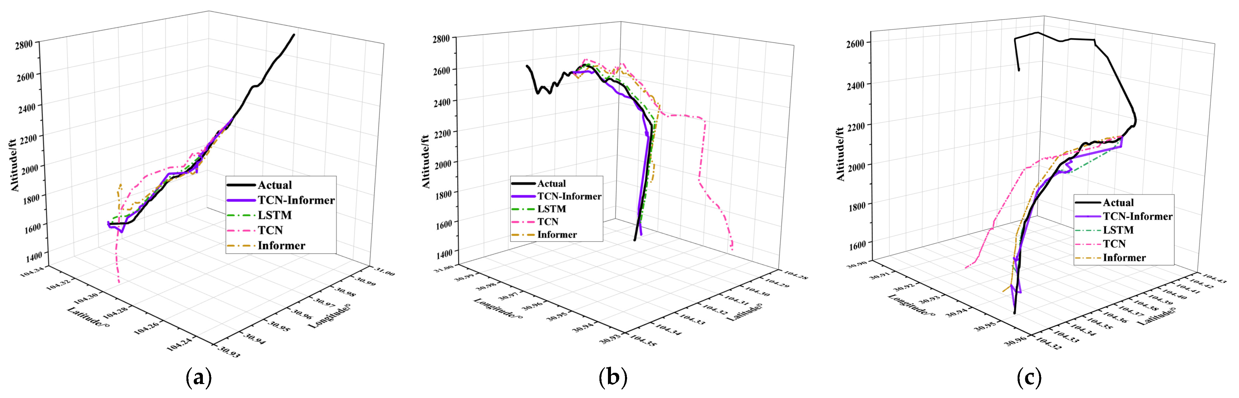
4.3.1. Visualization and Quantitative Analysis

In this study, the flight guidelines under the airport regulations mentioned in the Section 4.1.1 are used as an example for three actual approach phases with different flight subjects. Flight trajectories were different for each subject, so the three most common flight subjects were chosen as the background. In this study, the TCN, LSTM, Informer, and TCN-Informer architectures were used for the experimental simulation of the collected datasets, and the experimental results are shown (Figure 9 and Figure 10).

Figure 9. Predicted latitude, longitude, and altitude on the time axis for three subjects.

Figure 10. Trajectory prediction for the three subjects in three-dimensional coordinates. (a) Slow-Flight; (b) Basic Visual Flying; (c) Basic Instrument Flying.

The two-dimensional plots of the predicted trajectories in longitude, latitude, and altitude on the time axis are shown for the three flight subjects of slow-flight, basic visual flying, and basic instrument flying (Figure 9a–c). In all subjects, the predicted trajectories of the TCN-Informer architecture and LSTM model in longitude, latitude, and altitude coordinates maintain the same trend as the actual trajectory. The TCN-Informer architecture is not as smooth as the LSTM model in the graphs, but its predicted trajectory is very similar to the actual trajectory, with fewer fluctuations. From Figure 9, the Informer model starts with the same trend as the TCN-Informer architecture and LSTM model and begins to show a large deviation as time increases. However, the Informer model is slightly better than the TCN model from Figure 9. The TCN model provides the worst prediction results for longitude, latitude, and altitude data compared to the remaining models. From the 3D plots of the three subjects (Figure 10), the TP of both the TCN-Informer architecture and LSTM model is closest to the actual trajectory, followed by the Informer model and finally the TCN model. However, based on the evaluation metrics, the TCN-Informer architecture has a slightly higher prediction accuracy than the LSTM model. The results of the case tests represent a class of commonalities that can be utilized in the future for more flight trajectory prediction during the approach phase under different flight subjects.

4.3.2. Comparison of the Metric Error Values

Based on the visual comparison of the actual trajectory and the TP, as well as the analysis of the three evaluation indexes of MAE, RMSE, and MAPE, the integrated error value metrics are compared, as provided in Table 3.

Table 3. Comprehensive evaluation indicators for the different subjects.

Flight Subject	Model	MAE/°	RMSE/°	MAPE/%
Slow-Flight	TCN	32.1454	78.3910	7.9654
	LSTM	9.8064	25.3971	2.9366
	Informer	20.8752	58.0409	7.7361
	TCN-Informer	9.4425	20.8853	1.3440 × 10−3
Basic Visual Flying	TCN	28.5440	79.1948	2.6529
	LSTM	11.3799	29.5784	1.2906
	Informer	18.4654	46.3703	2.8452
	TCN-Informer	9.4923	25.1775	2.0402 × 10−3
Basic Instrument Flying	TCN	22.5312	55.4356	2.8083
	LSTM	11.2161	25.8144	1.9288
	Informer	13.1692	32.2399	2.2530
	TCN-Informer	7.6254	17.3124	8.5077 × 10−4

By analyzing Table 3, the following deduction can be drawn: for the three different flight subjects, the trajectory prediction errors of the TCN-Informer architecture are much lower than those of the TCN and Informer models in terms of the combined MAE, RMSE, and MAPE metrics. In the three subjects compared to those of TCN, the MAE values are reduced by 70.63%, 66.75%, and 66.16%. The RMSE values are reduced by 73.36%, 68.21%, and 68.77%. In the three subjects compared to LSTM, the MAE values are reduced by 3.71%, 16.58%, and 32.01%. The RMSE values are reduced by 17.77%, 14.88%, and 32.94%. In the three subjects compared to those of Informer, the MAE values are reduced by 54.77%, 48.60%, and 42.10%. The RMSE values are reduced by 64.01%, 45.70%, and 46.30%. The MAPE values of the TCN-Informer architecture are 1.3440 × 10⁻³, 2.0402 × 10⁻³, and 8.5077 × 10⁻⁴, respectively. Compared to the other predicted models, the MAPE values of the proposed model are minimized in three different flight subjects. This shows the high accuracy of the TCN-Informer architecture in the task of flight trajectory prediction. From the analysis of the results, the prediction accuracy of LSTM is second only to the TCN-Informer structure, then the Informer, and finally the TCN. Different magnitudes of data may have errors in the comprehensive evaluation index; thus, the individual evaluation indexes of each dimension need to be further analyzed. Table 4 shows the evaluation indicators for latitude, longitude, and altitude.

Table 4. Indicators for evaluating latitude, longitude, and altitude.

Flight Subject	Evaluation Metrics	Model	Longitude/°	Latitude/°	Altitude/ft
Slow-Flight	MAE	TCN	2.9475 × 10−3	5.4885 × 10−3	138.6668
		LSTM	4.5944 × 10−4	1.8136 × 10−3	41.5848
		Informer	2.5651 × 10−3	3.3762 × 10−3	82.8541
		TCN-Informer	2.2472 × 10−4	1.4018 × 10−3	37.9198
	RMSE	TCN	4.1494 × 10−3	8.2815 × 10−3	173.5556
		LSTM	6.8025 × 10−4	2.4814 × 10−3	46.0996
		Informer	3.1418 × 10−3	4.6291 × 10−3	128.1257
		TCN-Informer	2.4666 × 10−4	1.8077 × 10−3	45.9907
	MAPE/%	TCN	9.5224 × 10−3	5.2614 × 10−3	8.0965
		LSTM	1.4842 × 10−3	1.7386 × 10−3	2.4175
		Informer	8.2859 × 10−3	3.2364 × 10−3	5.1675
		TCN-Informer	1.3440 × 10−3	1.3440 × 10−3	1.3440 × 10−3
Basic Visual Flying	MAE	TCN	3.7299 × 10−3	6.7160 × 10−3	133.7629
		LSTM	5.7556 × 10−4	1.1042 × 10−3	52.0386
		Informer	7.1360 × 10−3	5.3758 × 10−3	76.0873
		TCN-Informer	4.1887 × 10−4	1.1028 × 10−3	39.3285
	RMSE	TCN	4.5117 × 10−3	7.9371 × 10−3	176.8146
		LSTM	6.2505 × 10−4	1.2624 × 10−3	65.9584
		Informer	9.7240 × 10−3	8.4468 × 10−3	101.6972
		TCN-Informer	2.5396 × 10−4	1.0554 × 10−3	55.4143
	MAPE/%	TCN	1.2044 × 10−2	6.4387 × 10−3	7.0794
		LSTM	1.8584 × 10−3	1.0586 × 10−3	2.7139
		Informer	2.3046 × 10−2	5.1537 × 10−3	3.7982
		TCN-Informer	1.6402 × 10−3	1.0402 × 10−3	2.0402 × 10−3
Basic Instrument Flying	MAE	TCN	2.1724 × 10−3	7.5674 × 10−3	102.9894
		LSTM	2.0974 × 10−4	2.9056 × 10−4	47.8487
		Informer	7.0690 × 10−4	5.2345 × 10−4	56.1740
		TCN-Informer	1.6903 × 10−4	1.1603 × 10−4	28.6839
	RMSE	TCN	2.8080 × 10−3	9.0990 × 10−3	123.4807
		LSTM	8.2249 × 10−4	7.7270 × 10−4	57.1074
		Informer	1.3013 × 10−3	2.9763 × 10−3	69.3845
		TCN-Informer	1.6903 × 10−4	5.1603 × 10−4	36.9918
	MAPE/%	TCN	7.0166 × 10−3	7.2549 × 10−3	5.5557
		LSTM	2.2829 × 10−3	5.0181 × 10−4	2.5899
		Informer	3.2415 × 10−3	2.5123 × 10−3	3.0203
		TCN-Informer	8.5076 × 10−4	8.5076 × 10−4	8.5076 × 10−4

Note that the MAE and RMSE units are units of the measured data, as shown in the table and MAPE are units of percent.

Based on Table 4, it can be concluded that the TCN-Informer architecture also outperforms the other models for single predictions in longitude, latitude, and altitude. The LSTM model is second only to the TCN-Informer architecture in terms of prediction. Under the slow-flight subject, the MAE values of the TCN-Informer architecture are reduced by 51.09%, 22.71%, and 8.81% for longitude, latitude, and altitude, respectively. The RMSE values decrease by 63.74%, 27.15%, and 0.23% for longitude, latitude, and altitude, respectively. Under the basic visual flying subject, the model showed a reduction in the MAE values of 27.22%, 0.13%, and 24.42% for longitude, latitude, and altitude, respectively. The RMSE was reduced by 59.37%, 16.40%, and 15.99% for longitude, latitude, and altitude, respectively. Under the basic instrument flying subject, the model showed a reduction in MAE of 19.41%, 60.07%, and 40.05% for longitude, latitude, and altitude, respectively. The RMSE values were reduced by 79.45%, 33.22%, and 35.22% for each. For three different flight subjects, the TCN-Informer architecture has the minimum MAPE metrics in longitude, latitude, and altitude prediction compared to those of the other models. Through a more detailed comparison, the high accuracy of the TCN-Informer framework in flight trajectory prediction is more evident in the error metrics analysis. The analysis of the evaluation indexes confirms the effectiveness and accuracy of the TCN-Informer architecture proposed in this study, which better meets the requirements of aircraft on the TP task.

4.4. Discussion

In this study, to improve the accuracy of TP, a hybrid TP model based on the TCN-Informer architecture is proposed. The proposed architecture is very sensitive to the training dataset because it belongs to the encoder-decoder architecture. Analyzing and quantifying the size of the dataset determines how well the model learns the trends of the flight trajectory changes and how effectively it works in terms of model training, so there are some limitations to the model. After the training and validation of the data after feature extraction, the most suitable dataset size and ratio are found.

To better validate the effectiveness and accuracy of the model, the approach trajectory views under three different subjects and the evaluation metrics of different models are used to analyze the TP results. The TCN-Informer architecture is compared with the single TCN model, the single Informer model, and the typical LSTM model widely used in previous studies. The results show that the TCN-Informer architecture achieves better prediction results through each evaluation index (Table 3 and Table 4). In terms of flight trajectory spatial position prediction, the predicted trajectory of the TCN-Informer architecture is generally consistent with the actual trajectory, indicating that the model is more effective in learning the trends of the flight trajectory changes and model training. Notably although the TCN-Informer architecture can alleviate the problem of large errors in TP to a certain extent, the errors are still large after the latitude and longitude coordinates are converted to actual distances. Second, in terms of altitude prediction on the time axis, the TCN-Informer architecture has a stable prediction effect with the lowest error range (Figure 9 and Figure 10), which shows the superiority of the medium- and long-term TP of our proposed model. Finally, we found that our improved model more effectively matches the actual flight trajectory for different subjects in the approach stage from the 3D graphs (Figure 9c and Figure 10c). Therefore, although our proposed architecture has outliers in the prediction results, the proposed architecture still shows great improvement for GA aircraft trajectory forecasting in the approach phase.

Although the proposed model is the best in terms of accuracy, it is inferior to supervised learning models such as TCN and LSTM in terms of computational efficiency. The model proposed in this research is a self-supervised learning model. The model treats the flight parameters as unlabeled data, and the training sample size for each flight subject is about two thousand, which in itself has some limitations and makes the computational efficiency low. Therefore, improving the computational efficiency of self-supervised learning in flight trajectory prediction can be a future research goal. Due to the slightly different labeling information of other prediction algorithms, the complexity of the network design, and the open-source nature of the research, studying and comparing other flight trajectory prediction methods will be the future research direction. Overall, the proposed model provides a foundation for future research in terms of methodological innovation.

5. Conclusions and Future Research

In this study, a hybrid TP model based on TCN and the Informer architecture is proposed by utilizing historical flight trajectory data. In the TP task, feature extraction on the sequential trajectory data through the TCN model is effectively performed, and the Informer model is then used to predict the trajectory of multiple future moments at a time. The performance of our proposed method is demonstrated by various comparative analyses. The accuracy of the prediction model is measured via MAE, RMSE, and MAPE metrics. The results verify that the TCN model can effectively improve prediction performance and avoid common problems in recurrent neural networks such as gradient explosion/vanishing or lack of memory retention. Moreover, our proposed TCN-Informer architecture outperforms the widely used typical models in terms of its ability to predict medium and long series of flight trajectory data.

To avoid accidents and ensure the safety of general aviation, the TP in the approach phase needs to be considered. Accurate prediction can reduce the occurrence rate of dangerous accidents as well as the probability of go-arounds. This prediction not only ensures flight safety but also reduces fuel consumption, which is favorable to the sustainable development of general aviation. Future research can focus on exploring solutions to anomaly detection in the TP with the TCN-Informer architecture. In addition, more suitable methods for feature extraction on spatiotemporal data are needed to improve the efficiency and accuracy of model prediction.

References

- Wang, C.; Hu, M.; Yang, L.; Zhao, Z. Prediction of air traffic delays: An agent-based model introducing refined parameter estimation methods. PLoS ONE 2021, 16, e0249754. [Google Scholar] [CrossRef]
- Valasek, J.; Harris, J.; Pruchnicki, S.; McCrink, M.; Gregory, J.; Sizoo, D.G. Derived angle of attack and sideslip angle characterization for general aviation. J. Guid. Control Dyn. 2020, 43, 1039–1055. [Google Scholar] [CrossRef]
- Sailaranta, T.; Siltavuori, A. Stability Study of the Accident of a General Aviation Aircraft. J. Aerosp. Eng. 2018, 31, 06018001. [Google Scholar] [CrossRef]
- Schwarz, C.W.; Fischenberg, D.; Holzäpfel, F. Wake turbulence evolution and hazard analysis for general aviation takeoff accident. J. Aircr. 2019, 56, 1743–1752. [Google Scholar] [CrossRef]
- Fultz, A.J.; Ashley, W.S. Fatal weather-related general aviation accidents in the United States. Phys. Geogr. 2016, 37, 291–312. [Google Scholar] [CrossRef]
- Vilardaga, S.; Prats, X. Operating cost sensitivity to required time of arrival commands to ensure separation in optimal aircraft 4D trajectories. Transp. Res. Part C Emerg. Technol. 2015, 61, 75–86. [Google Scholar] [CrossRef]
- Tian, Y.; He, X.; Xu, Y.; Wan, L.; Ye, B. 4D trajectory optimization of commercial flight for green civil aviation. IEEE Access 2020, 8, 62815–62829. [Google Scholar] [CrossRef]
- Masi, G.; Amprimo, G.; Ferraris, C.; Priano, L. Stress and Workload Assessment in Aviation—A Narrative Review. Sensors 2023, 23, 3556. [Google Scholar] [CrossRef] [PubMed]
- Jiang, S.-Y.; Luo, X.; He, L. Research on method of trajectory prediction in aircraft flight based on aircraft performance and historical track data. Math. Probl. Eng. 2021, 2021, 6688213. [Google Scholar] [CrossRef]
- Obajemu, O.; Mahfouf, M.; Maiyar, L.M.; Al-Hindi, A.; Weiszer, M.; Chen, J. Real-time four-dimensional trajectory generation based on gain-scheduling control and a high-fidelity aircraft model. Engineering 2021, 7, 495–506. [Google Scholar] [CrossRef]
- Salahudden, S.; Joshi, H.V. Aircraft trajectory generation and control for minimum fuel and time efficient climb. Proc. Inst. Mech. Eng. Part G J. Aerosp. Eng. 2023, 237, 1435–1448. [Google Scholar] [CrossRef]
- Yuan, L.H.; Wang, L.D.; Xu, J.T. Adaptive fault-tolerant controller for morphing aircraft based on the L2 gain and a neural network. Aerosp. Sci. Technol. 2023, 132, 107985. [Google Scholar] [CrossRef]
- Ma, L.; Tian, S. A hybrid CNN-LSTM model for aircraft 4D trajectory prediction. IEEE Access 2020, 8, 134668–134680. [Google Scholar] [CrossRef]
- Shi, Z.; Xu, M.; Pan, Q. 4-D flight trajectory prediction with constrained LSTM network. IEEE Trans. Intell. Transp. Syst. 2020, 22, 7242–7255. [Google Scholar] [CrossRef]
- Guo, D.; Wu, E.Q.; Wu, Y.; Zhang, J.; Law, R.; Lin, Y. Flightbert: Binary encoding representation for flight trajectory prediction. IEEE Trans. Intell. Transp. Syst. 2022, 24, 1828–1842. [Google Scholar] [CrossRef]
- Jia, P.; Chen, H.; Zhang, L.; Han, D. Attention-lstm based prediction model for aircraft 4-d trajectory. Sci. Rep. 2022, 12, 15533. [Google Scholar] [CrossRef]
- Wang, Z.-S.; Zhang, Z.-Y.; Cui, Z. Research on Resampling and Clustering Method of Aircraft Flight Trajectory. J. Signal Process. Syst. 2022, 95, 319–331. [Google Scholar] [CrossRef]
- Zhao, Y.; Li, K. A Fractal Dimension Feature Model for Accurate 4D Flight-Trajectory Prediction. Sustainability 2023, 15, 1272. [Google Scholar] [CrossRef]
- Jin, X.; Yu, X.; Wang, X.; Bai, Y.; Su, T.; Kong, J. Prediction for Time Series with CNN and LSTM. In Proceedings of the 11th International Conference on Modelling, Identification and Control (ICMIC2019), Tianjin, China, 13 July 2019; Springer: Singapore, 2020; pp. 631–641. [Google Scholar]
- Chan, S.; Oktavianti, I.; Puspita, V. A deep learning cnn and ai-tuned svm for electricity consumption forecasting: Multivariate time series data. In Proceedings of the IEEE 10th Annual Information Technology, Electronics and Mobile Communication Conference (IEMCON), Vancouver, BC, Canada, 17–19 October 2019; pp. 488–494. [Google Scholar]
- Bai, S.; Kolter, J.Z.; Koltun, V. An empirical evaluation of generic convolutional and recurrent networks for sequence modeling. arXiv 2018, arXiv:1803.01271. [Google Scholar]
- Long, J.; Shelhamer, E.; Darrell, T. Fully convolutional networks for semantic segmentation. In Proceedings of the 2015 IEEE Conference on Computer Vision and Pattern Recognition, Boston, MA, USA, 7–12 June 2015; pp. 3431–3440. [Google Scholar] [CrossRef]
- Yuan, R.; Abdel-Aty, M.; Gu, X.; Zheng, O.; Xiang, Q. A Unified Approach to Lane Change Intention Recognition and Driving Status Prediction through TCN-LSTM and Multi-Task Learning Models. arXiv 2023, arXiv:2304.13732. [Google Scholar]
- Zhou, H.; Li, J.; Zhang, S.; Yan, M.; Xiong, H. Expanding the prediction capacity in long sequence time-series forecasting. Artif. Intell. 2023, 318, 103886. [Google Scholar] [CrossRef]
- Xu, H.; Peng, Q.; Wang, Y.; Zhan, Z. Power-Load Forecasting Model Based on Informer and Its Application. Energies 2023, 16, 3086. [Google Scholar] [CrossRef]
- An, Z.; Cheng, L.; Guo, Y.; Ren, M.; Feng, W.; Sun, B.; Ling, J.; Chen, H.; Chen, W.; Luo, Y.; et al. A novel principal component analysis-informer model for fault prediction of nuclear valves. Machines 2022, 10, 240. [Google Scholar] [CrossRef]
- Yang, Z.; Liu, L.; Li, N.; Tian, J. Time series forecasting of motor bearing vibration based on informer. Sensors 2022, 22, 5858. [Google Scholar] [CrossRef]
- Ma, J.; Dan, J. Long-Term Structural State Trend Forecasting Based on an FFT–Informer Model. Appl. Sci. 2023, 13, 2553. [Google Scholar] [CrossRef]
- Ren, Y.; Wang, S.; Xia, B. Deep learning coupled model based on TCN-LSTM for particulate matter concentration prediction. Atmos. Pollut. Res. 2023, 14, 101703. [Google Scholar] [CrossRef]
Disclaimer/Publisher’s Note: The statements, opinions and data contained in all publications are solely those of the individual author(s) and contributor(s) and not of MDPI and/or the editor(s). MDPI and/or the editor(s) disclaim responsibility for any injury to people or property resulting from any ideas, methods, instructions or products referred to in the content. |
© 2023 by the authors. Licensee MDPI, Basel, Switzerland. This article is an open access article distributed under the terms and conditions of the Creative Commons Attribution (CC BY) license (https://creativecommons.org/licenses/by/4.0/).