Assessment of Ecological Flow in Hulan River Basin Utilizing SWAT Model and Diverse Hydrological Approaches

Abstract

Human activities have significantly altered the hydrological processes of rivers. In recent years, the increased focus on global water resource exploitation and land use changes has heightened the significance of related ecological and environmental issues. To investigate the land use changes in Hulan River Basin between 1980 and 2020, and the corresponding flow under various ecological standards, a quantitative assessment of land use changes in Hulan River Basin was conducted by analyzing the Land Use Dynamic Degree (LUD) index and the land use change matrix. Two types of models, namely natural runoff models and status quo runoff models, were developed to evaluate alterations in basin runoff. Various hydrological techniques were utilized to calculate the ecological water deficit in Hulan River Basin. The results suggest the following: (1) human consumption comprises approximately 40% of surface water resources, with Hulan River Basin exhibiting a moderate consumption level; (2) when determining the minimum ecological flow, the Distribution Flow Method (DFM) method yielded slightly higher outcomes compared to alternative methodologies; both the variable Q₉₀ method and DFM (Q₂) method satisfy 10% of the natural river flow, however, in terms of capturing the hydrological pattern, DFM exhibits a slightly lower fitting degree compared to the variable Q₉₀ (monthly average flow with 90% guarantee rate) method; (3) DFM is identified as scientifically reasonable for determining the most suitable ecological flow in comparison to other hydrological methods; (4) despite the widespread water scarcity in Hulan River Basin, the variance between most periods and the ideal ecological flow remains minimal, indicating that severe water shortages are uncommon.

1. Introduction

In recent years, escalating human water consumption has brought attention to ecological concerns within river basins [1]. The impact of societal and agricultural water utilization on river flow has resulted in alterations in the hydrological patterns and ecosystem functions of rivers [2,3]. The decrease in riverine ecological functions has elicited public concern regarding ecological flow [4]. The systematic and scientific assessment of riverine ecological flow serves to advance the judicious utilization of water resources and the rehabilitation of riverine ecological functions, thereby enhancing the efficacy of water resource utilization [5]. This aspect is essential for preserving the overall integrity of the basin’s ecological functions and ecosystem structure [6].

In China, significant advancements have been made in the field of hydrology regarding the hydrological calculation methods for ecological flow and the techniques for natural runoff reconstruction, as outlined in Table 1. The Ministry of Water Resources of China issued “Specification for Calculation of Ecological Water Demand in River and Lake Ecosystems” (SL/T 712-2021 [7]) in 2021. This specification delineates the essential ecological flow of rivers as the minimum volume necessary to uphold the ecological functions of rivers, lakes, and wetlands and to accomplish precise ecological protection goals. The exploration of ecological flow in China can be traced back to the 1970s, when Tang and Chen [8] introduced the concepts of “ensuring water for the ecological environment of each oasis” and “ecological environmental water” in research on water resources and oasis development in Tarim Basin. Meng et al. [9] proposed a modular simulation model designed for ecological–habitat–flow considerations, specifically tailored to address the different demands of river ecosystems. Zheng et al. [10] employed ecological flow as a hydrological parameter to evaluate the ecological well-being of four tributaries within Weihe River system. They utilized a biological–habitat methodology, with zooplankton serving as indicator organisms. Wang et al. [11] developed a predictive model for ecological flow early warnings in Jiaojiang River Basin. The model utilized Long Short-Term Memory (LSTM) neural networks in combination with entropy methods, demonstrating the model’s appropriateness and efficacy in providing warning signals for ecological flow. Tian et al. [12] improved the annual distribution method and implemented it in the northwest river region. Their study revealed that seasonal modifications to the annual distribution method are better suited for this specific region.

Previous studies for calculating ecological flow have primarily focused on determining the ecological flow in the main river or at the basin outlet, neglecting a systematic approach for assessing the spatial and temporal distribution of water scarcity across the entire basin. The watershed water system is a comprehensive entity characterized by intricate interconnections among different sub-watersheds. Achieving a balanced ecological water replenishment necessitates a combination of point and surface approaches [13], top-down connectivity, and multi-objective coordination. Therefore, it is essential to conduct an analysis and assessment of the spatial and temporal distribution of ecological flow and water scarcity throughout the entire watershed [14,15].

The Distribution Flow Method (DFM) offers an advantage in reducing the impact of extreme runoff values on the calculation of ecological flow. Obtaining over 30 years of daily natural runoff data is often necessary, a task that can be challenging due to the extensive time period involved. The main objectives of this study include the following: (1) evaluating the suitability of DFM in Hulan River Basin; (2) utilizing the Soil and Water Assessment Tool (SWAT) model to define the natural runoff patterns of Hulan River to meet the data demands of DFM; (3) employing the SWAT model to differentiate between the natural runoff and current runoff processes of Hulan River, categorizing them into flood and non-flood periods. Drawing upon watershed ecological flow theory, the overall objective of this study is to finalize the computation of ecological flow throughout the entirety of Hulan River Basin and assess the prevailing ecological water scarcity conditions within the basin.

Hulan River, a significant tributary of Songhuajiang River, is situated on the left bank of Songhuajiang River in the central area of Heilongjiang Province. It constitutes around 6.56% of the total Songhua River basin area, positioning it as the third largest tributary within the basin. The region is characterized by a temperate continental monsoon climate, with an average annual precipitation of 574.7 mm. Precipitation is unevenly distributed, with the majority occurring between June and September. Hulan River covers a total area of 35,683 km², establishing it as the largest river that is entirely situated within Heilongjiang Province [16]. Hulan River plays a crucial role in supplying water for residents and irrigating farmland within the basin [17]. Therefore, the ecological security of Hulan River is intricately linked to the social and economic development of the area, as well as to the water usage patterns of the residents within the basin. An overview map of Hulan River Basin is illustrated in Figure 1.

Table 1. Literature review of methodologies for estimating natural runoff and calculating ecological flow.

Study Area	Method	Research Focus	References
Taohe River	Runoff component investigation method	Identified runoff variation characteristics, highlighting the impact of current runoff calculations on ecological flow strategies.	[18]
Fenhe River	SWAT model and Tennant method	Explored ecological water supplement strategies, utilizing SWAT Model for effective water management.	[19]
Xibei River	Improved annual distribution method	Analyzed river ecological flow using an enhanced distribution approach, offering insights into water allocation and conservation.	[12]
Xishui River	Runoff component investigation method and SWAT model	Assessed water resources through integrated runoff investigation and modeling, facilitating comprehensive water resource management.	[20]
Hanjiang River	SWAT model and cellular automata	Examined the evolution of ecological flow characteristics under environmental changes, emphasizing adaptive management strategies.	[4]
Yellow River	Mann–Kendall test and double cumulative curve method	Investigated natural runoff reduction and consistency treatment methods, proposing solutions for sustainable river basin management.	[21]
Hei River	Heuristic segmentation method and various hydrological methods	Evaluated minimum and suitable ecological flows, considering hydrological variability for inland basin sustainability.	[22]
Yichang Section of Yangtze River	DFM and various hydrological methods	Determined ecological water requirements, leveraging DFM for ecological balance.	[23]
Long River	Physical habitat simulation and Penman–Monteith equation	Conducted quantitative ecological flow calculations, advocating for nature-based solutions in water resource optimization.	[24]

Table 1. Literature review of methodologies for estimating natural runoff and calculating ecological flow.

Study Area	Method	Research Focus	References
Taohe River	Runoff component investigation method	Identified runoff variation characteristics, highlighting the impact of current runoff calculations on ecological flow strategies.	[18]
Fenhe River	SWAT model and Tennant method	Explored ecological water supplement strategies, utilizing SWAT Model for effective water management.	[19]
Xibei River	Improved annual distribution method	Analyzed river ecological flow using an enhanced distribution approach, offering insights into water allocation and conservation.	[12]
Xishui River	Runoff component investigation method and SWAT model	Assessed water resources through integrated runoff investigation and modeling, facilitating comprehensive water resource management.	[20]
Hanjiang River	SWAT model and cellular automata	Examined the evolution of ecological flow characteristics under environmental changes, emphasizing adaptive management strategies.	[4]
Yellow River	Mann–Kendall test and double cumulative curve method	Investigated natural runoff reduction and consistency treatment methods, proposing solutions for sustainable river basin management.	[21]
Hei River	Heuristic segmentation method and various hydrological methods	Evaluated minimum and suitable ecological flows, considering hydrological variability for inland basin sustainability.	[22]
Yichang Section of Yangtze River	DFM and various hydrological methods	Determined ecological water requirements, leveraging DFM for ecological balance.	[23]
Long River	Physical habitat simulation and Penman–Monteith equation	Conducted quantitative ecological flow calculations, advocating for nature-based solutions in water resource optimization.	[24]

2. Data and Methods

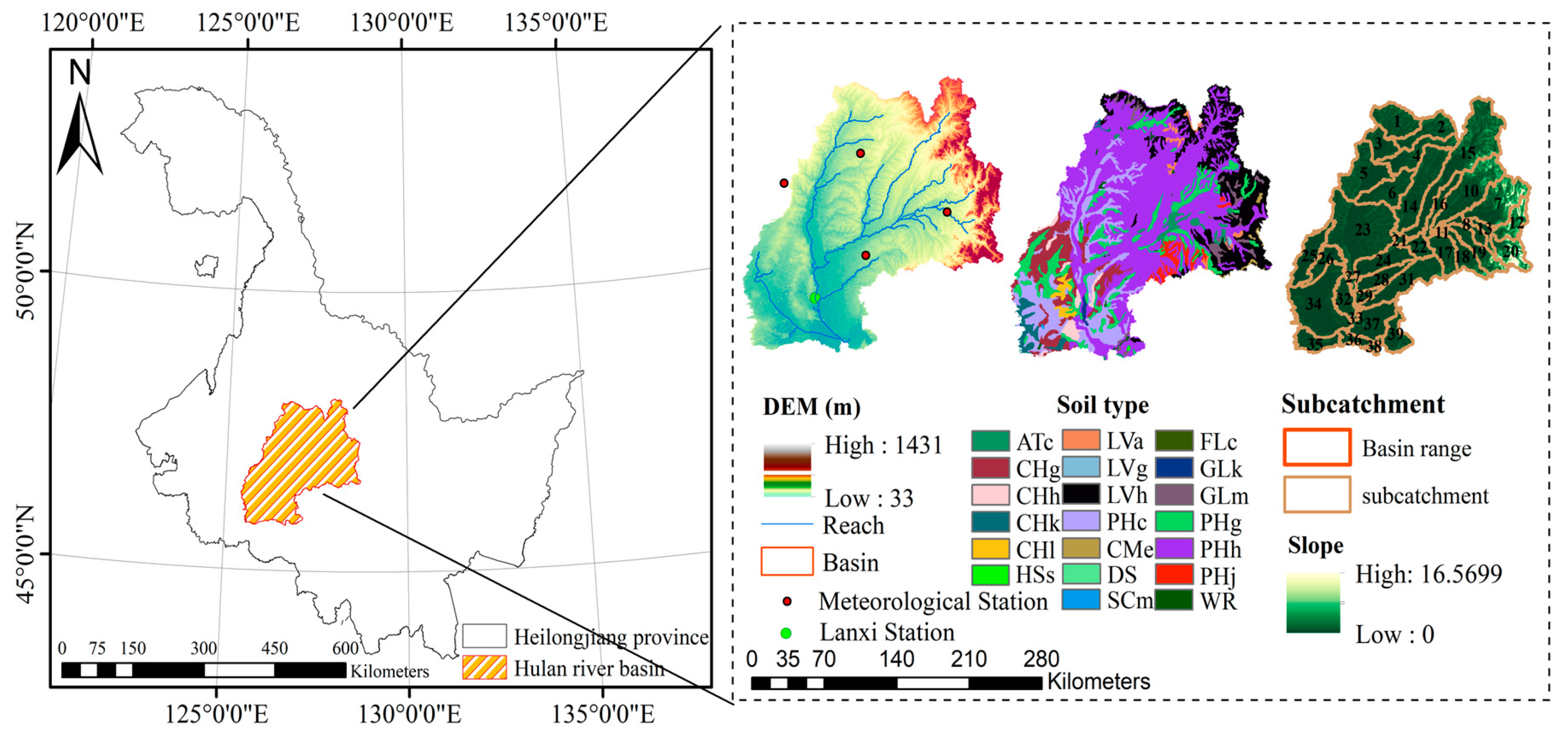
2.1. Data Source and Processing

2.1.1. Digital Elevation Model (DEM)

The research suggests that selecting an optimal resolution of 20–150 m is advisable for elevation data when using SWAT for runoff simulation [25]. In this study, the DEM data used were obtained from Geographic Spatial Data Cloud platform (https://www.gscloud.cn/, accessed on 21 January 2024). The data had a resolution of 30 m and were derived from Shuttle Radar Topography Mission (SRTM) elevation data. DEM was utilized to derive relevant parameters for Heilongjiang River Basin (Figure 1).

2.1.2. Meteorological Data

The measured data (precipitation, temperature, wind speed, relative humidity, solar radiation) from four fundamental meteorological stations within Hulan River Basin, namely Suihua Beilin District Basic Meteorological Station (station number 50853), Hailun Basic Meteorological Station (station number 50756), Tieling Basic Meteorological Station (station number 50862), and Mingshui Basic Meteorological Station (station number 50758), were obtained by accessing the data from China National Meteorological Data Center (http://data.cma.cn/, accessed on 21 January 2024). The temporal scope of meteorological data ranges from 1960 to 2020, covering a total duration of 60 years. Subsequently, a meteorological database was constructed for subsequent analysis and research purposes. The primary meteorological station’s location is depicted in Figure 1.

2.1.3. Hydrological Data

The hydrological data chosen for this investigation consist of daily streamflow records collected at Lanxi hydrological station in Hulan River Basin, spanning from 1964 to 1971 and from 2008 to 2022. The data continuity within this timeframe is deemed satisfactory, rendering it appropriate for model calibration and validation processes. Figure 1 represents the hydrological station’s location.

2.1.4. Land Use

Land use data play a pivotal role in developing the SWAT model, as they significantly impact the hydrological mechanisms by which precipitation induces runoff on land surfaces [26,27,28,29]. The land use data utilized in this study were sourced from the Data Platform of Resource and Environment Science and Data Center of Chinese Academy of Sciences (http://www.resdc.cn, accessed on 21 January 2024). The study encompasses the time frame from 1980 to 2020, with 10-year intervals. Prior to utilization, the data need to be structured into a table indicating the land use index. Figure 2 depicts the land use map of Hulan River Basin from 1980 to 2020. The meaning of the land use abbreviation is shown in

Table 2. Classification and abbreviations of land use categories.

Abbreviation	Land Use Category
AGRL	Agricultural Land
FRST	Forest
PAST	Pasture
WATR	Water Body
URML	Residential—Medium/Low Density
URLD	Residential—Low Density
UIDU	Industrial Land
BARR	Bare Land

.

2.1.5. Soil Type

Soil data are essential as a primary input parameter in the SWAT model, and the accuracy of soil data will significantly impact the simulation outcomes of the model. The spatial distribution map of soil types in Hulan River Basin is obtained from the Harmonized World Soil Database (HWSD) [30]. Prior to the establishment of the soil database, it is crucial to employ SWAT for the computation of diverse physical and chemical attributes of the soil and for the reclassification of the soil within the designated research area [31]. The soil types present in Hulan River Basin are illustrated in Figure 1. Abbreviations and explanations of soil types are shown in

Table 3. Soil types and abbreviations within study area.

Abbreviation	Soil Type	Abbreviation	Soil Type
ATc	Cumulic Anthrosols	CMe	Eutric Cambisols
CHg	Gleyic Chernozems	DS	Dunes and Shift Sands
CHh	Haplic Chernozems	SCm	Mollic Solonchaks
CHk	Calcic Chernozems	FLc	Calcaric Fluvisols
CHl	Luvic Chernozems	GLk	Calcic Gleysols
HSs	Terric Histosols	GLm	Mollic Gleysols
LVa	Albic Luvsiols	PHg	Gleyic Phaeozems
LVg	Gleyic Luvisols	PHh	Haplic Phaeozems
LVh	Haplic Luvisols	PHj	Stagnic Phaeozems
PHc	Calcaric Phaeozems	WR	Water Bodies

2.2. Land Use Dynamic Degree (LUD) Index

The LUD index is characterized as the proportion of the alteration in a particular land use category during a specified timeframe, focusing on the speed of change of that specific land use category. It functions as a metric for evaluating the degree of human development, utilization, or conservation of a particular land use category within a specified timeframe. The calculation for LUD index is depicted in Equation (1) as follows.

The Comprehensive Land Use Dynamic Degree (CLUD) index is calculated as the aggregate of the absolute values of the individual dynamic degrees associated with all land use types within a defined geographical area during a specific time frame. This metric offers valuable insights into the magnitude of changes in land use types within the region. The calculation for CLUD index is determined through Equation (2) as follows:

$$K=\frac{U_b-U_a}{U_a}\times \frac{1}{T}\times 100\mathrm{\%}$$

(1)

$$LC=\frac{\sum _{i=1}^n\mathsf{\Delta }L{U}_{i-j}}{2\sum _{i=1}^{n}L{U}_i}\times \frac{1}{T}\times 100\mathrm{\%}$$

(2)

where K represents a single land use dynamic attitude; U_a and U_b represent the initial and final area of a single land use type; T represents the change time period; LC represents the comprehensive land use dynamic attitude; $\mathsf{\Delta }L{U}_{i-j}$ represents the absolute value of the area of land class i converted to non-i land class during time T; and $L{U}_i$represents the initial area of land class i.

2.3. Land Use Transfer Matrix

The land use transfer matrix method is a technique that utilizes the Markov model for examining the dynamics of changes in land use. This approach allows for the measurement of shifts between different land use categories. The computational algorithm is represented by Equation (3) as follows:

$$S_{ij}=\left[\begin{array}{ccc}{S}_{12}& \cdots & S_{1n}\\ ⋮& \ddots & ⋮\\ S_{n1}& \cdots & S_{nn}\end{array}\right]$$

(3)

where S represents the area; n represents the number of land use types before and after conversion; i and j (i, j = 1, 2, …, n) represent the land types before and after conversion, respectively; and S_ij represents the area of land type i converted to land type j before the conversion.

2.4. SWAT Model

SWAT is a physical–conceptual model that employs the water balance as the primary mechanism for each process. It is suitable for conducting extended investigations into hydrological and biogeochemical cycles [32,33]. The model functions by partitioning the watershed into Hydrological Response Units (HRUs), analyzing the internal cycles within each unit independently, and subsequently integrating these units through sub-basins and river networks. The SWAT model is predominantly employed for evaluating the enduring effects of human activities, such as land use management, on watershed hydrology, sediment transport, and the migration of agricultural pollutants [34,35]. The first step in developing the model includes delineating sub-basins (Figure 1). Subsequently, areas with comparable combinations of land use types, soil types, and slopes are subdivided into HRUs based on the sub-basins [36]. The cumulative output of each HRU is consolidated at the sub-basin outlet. Meteorological data are processed using SWAT weather to interpolate missing values in measured data and generate a data index table for input into the SWAT simulation [37].

This study utilized the correlation of coefficient (R²) and Nash–Sutcliffe efficiency coefficient (NSE) to assess the applicability of the SWAT model in the Hulan River Basin. The Nash–Sutcliffe efficiency (NSE) and the coefficient of correlation (R²) are as follows:

$$NSE=1-\frac{{\sum }_{i=1}^n{\left(Q_i^{obs}-Q_i^{sim}\right)}^2}{{\sum }_{i=1}^n{\left(Q_i^{obs}-Q_{mean}^{obs}\right)}^2}$$

(4)

$$R^2=\frac{{\left({\sum }_{i=1}^n\left(Q_i^{obs}-Q_{mean}^{obs}\right)\times \left(Q_i^{sim}-Q_{mean}^{sim}\right)\right)}^2}{{\sum }_{i=1}^n{\left(Q_i^{obs}-Q_{mean}^{obs}\right)}^2\times {\sum }_{i=1}^n{\left(Q_i^{sim}-Q_{mean}^{\mathrm{s}\mathrm{i}\mathrm{n}}\right)}^2}$$

(5)

where $Q_i^{obs}$ is the measured value, $Q_i^{sim}$ is the simulated value, $Q_{mean}^{obs}$ is the mean observed value, and $Q_{mean}^{\mathrm{s}\mathrm{i}\mathrm{n}}$ is the mean simulated value.

2.5. Itemized Survey Method

This study employed the SWAT model to simulate natural runoff and utilized a sub-item survey method to validate the results of the natural runoff model simulation. The calculation for the sub-item survey method is expressed as follows [18,20]:

W_nature = W_measured + W_irrigate + W_industrial + W_domestic + W_reservoir ± W_diversion

(6)

where W_nature represents the natural runoff; W_measured represents the measured runoff; W_irrigation represents the irrigation water volume; W_industrial represents the industrial water usage; W_domestic represents the domestic water usage; W_reservoir represents the reservoir storage variation; and W_diversion represents the water diversion or transfer in hydraulic engineering projects.

2.6. Runoff Simulation and the Division of Flood and Drought Periods in Watershed

Utilizing Mann–Whitney–Pettitt change point analysis, prior research has identified a statistically significant change point in the annual runoff of Hulan River Basin in 1972 at a significance level of 0.05 [38]. This implies that human activities had a negligible effect on the runoff in Hulan River Basin before 1972. Subsequently, the calibrated parameters of the hydrological model prior to the change point were employed to incorporate the observed meteorological data of the sample basin into the SWAT model. The simulated flow process from 1990 to 2020 may be regarded as a natural flow process with minimal human impact. Hydrological models were developed for the natural runoff and status quo runoff in Hulan River Basin based on land use data from 1980 and 2020. Model calibration for natural runoff was carried out from 1964 to 1967, whereas model validation was conducted from 1967 to 1971. For the status quo runoff scenario, model calibration was performed for the period spanning from 2008 to 2013, followed by validation from 2013 to 2020. The calibrated hydrological model parameters were subsequently incorporated into the SWAT model, together with observed meteorological data, within Hulan River Basin. The natural runoff data from 1990 to 2020, acquired from the natural runoff model in Hulan River Basin, were segmented into wet and dry periods utilizing the Cumulative Anomaly Method (CAM) [39]. Finally, average and index curve graphs depicting monthly average flow cumulative anomalies in Hulan River Basin were generated through the application of a specific calculation method for runoff cumulative anomalies:

$$\overline{Q_l}=\frac{1}{m}{\sum }_{\tau =1}^m{Q}_{l,\tau }$$

(7)

$$S_{l,\tau }={\sum }_{t=1}^{\tau }\left(Q_{l,t}-{\overline{Q}}_l\right)$$

(8)

$$k_l^{+}=\frac{\mathit{max}\left(S_{l,\tau }\right)+\mathit{min}\left(S_{l,\tau }\right)}{\overline{{\mathrm{Q}}_l}}$$

(9)

$$\overline{k_{T_0}^{+}}=\frac{1}{N}{\sum }_{l=1}^N{k}_l^{+}$$

(10)

this study determines the flow of $Q_{l,t}$ in each unit time period, where m represents the number of units in a year; $\overline{Q_l}$ represents the average flow of the $l$ hydrological year ($l$ = 1,2,...,N; N = n−1 when T₀ ≠ 1 and N = n when T₀ = 1); $S_{l,\tau }$ represents the cumulative departure from the mean flow for each time period; $k_l^{+}$ represents the total exponent of the cumulative departure from the mean flow; $\overline{k_{T_0}^{+}}$ represents the average total exponent of the cumulative departure from the mean flow.

2.7. Ecological Flow Calculation

The natural streamflow data used in this study originate from the simulated results of a SWAT-based model for natural streamflow in Hulan River Basin, as described in Section 2.4. The dataset covers the period from 1990 to 2020, constituting a total timespan of 30 years. The model employed the daily runoff data recorded at Lanxi hydrological station in Hulan River Basin from 1964 to 1971 for comprehensive calibration and validation. The results suggest that the model adequately represents the natural runoff dynamics in Hulan River Basin, indicating its appropriateness for calculating ecological flow.

2.7.1. Distribution Method

The methodology used to calculate the annual flow distribution is based on the comprehensive dataset of natural runoff obtained from hydrological stations located within the basin. The annual average value Q_min of the minimum monthly runoff and the multi-year average monthly runoff Q are computed and, subsequently, the ratio between them is derived to yield the concurrent mean ratio η. By incorporating the concurrent mean ratio coefficient with the multi-year average runoff qj (j = 1~12), the ultimate ecological flow is determined for each month. The crucial element of this methodology is centered on calculating the concurrent mean ratio. However, the absence of flow in specific months, along with instances of extreme runoff events, could impact the minimum monthly runoff and thereby have an impact on the outcomes. Furthermore, the methodology fails to consider seasonal fluctuations in multi-year runoff when conducting the calculation process. The application of this method in rivers characterized by significant seasonality may result in considerable deviations. Therefore, taking into account the distinctive features of Hulan River, this research utilizes the enhanced annual flow distribution technique introduced by Tian et al. [12], which integrates seasonal segmentation into the computation procedure. The table presents the seasonal division of Hulan River, accompanied by the corresponding calculation equation.

$${\overline{Q}}_{90\mathrm{\%},i}=\frac{1}{t_i}{\sum }_j^{t_i}{q}_{90\mathrm{\%},ij}$$

(11)

$$S_{l,\tau }={\sum }_{t=1}^{\tau }\left(Q_{l,t}-{\overline{Q}}_l\right)$$

(12)

$${\eta }_i=\frac{{\overline{Q}}_{90\mathrm{\%},i}}{{\overline{Q}}_i}$$

(13)

where q_90%,ij represents the monthly runoff volume for the j-th month of the i-th time period at a 90% confidence level, m³/s; t_i is the number of months corresponding to period i, $\sum _{i=1}^n{t}_i=12$; ${\overline{Q}}_{90\%}$ is the average monthly runoff at different time periods under a 90% guarantee rate, m³/s; ${\overline{q}}_{ij}$ is the multi-year average runoff for the i time period in the j month, m³/s; Q_i is the average monthly runoff of each period i, m³/s; η_i is the enhancing same-period mean ratio for different time periods i, i = 1,2,…, n(n ≤ 4); and j = 1,2,…,12.

2.7.2. Monthly Minimum Method

The minimum dilution volume for water purification, also known as the dilution capacity, is employed to assess the pollution load capacity of river water bodies based on the natural monthly mean flow rate. When dealing with rivers that are covered with ice, it is advisable to select a non-zero minimum monthly mean flow rate as the reference point. In this study, the natural monthly mean flow rate is utilized as the fundamental basis, and frequency analysis is conducted by employing the mean flow rate of the driest month within a standard hydrological year.

2.7.3. The Texas Method

The Texas method, referred to as Environmental Flow Standard, was enacted by the legislative authority of the state of Texas in 2007 [40]. This method takes into account the seasonal variations in river discharge and specifies that a certain percentage of the natural monthly mean discharge, with a 50% assurance rate, is allocated as the ecological base flow. Drawing upon the research contributions of various national scholars, the ecological base flow is determined as 30% of the natural monthly mean discharge at the 50% assurance rate [41].

2.7.4. Q₅₀–Q₉₀

The Q₅₀–Q₉₀ method is also referred to as the monthly frequency calculation method. This method classifies the ecological status of rivers into four categories. Q₅₀ represents the monthly flow at 50% frequency density and serves as an indicator of a positive ecological flow status. Q₇₅ denotes the monthly flow occurring at 75% frequency density, indicating a moderate ecological status. Q₉₀ represents the monthly flow occurring at 90% frequency density and is acknowledged as the essential ecological flow requirement [42]. Rivers that do not meet Q₉₀ criteria are considered to be experiencing ecological degradation.

2.7.5. The Tessman Method

The Tessman method, introduced by Tessman in 1980 to estimate river ecological flow, has emerged as a prominent approach in eco-hydrological computations. When the monthly mean discharge values are less than 40% of the annual mean discharge values for multiple years, they are classified as ecological flow. If the monthly mean discharge values fall between 40% and 100% of the annual mean discharge values for multiple years, 40% of the annual mean discharge values are considered as ecological flow. When monthly mean discharge values surpass annual averages over several years, 40% of these monthly averages are designated as ecological flows [43].

2.7.6. The DFM Method

The DFM (Distribution Flow Method), introduced by Tian et al [12]., utilizes Vermeesch’s variable kernel density function to simulate the Antecedent Precipitation Index (API) of monthly streamflow. This approach provides a framework for estimating the distribution function of variable kernel density flow sequences. This method is proficient in assessing the degree of satisfaction of streamflow in river ecosystems, thus indicating the ecological health and spatial–temporal patterns of different flow magnitudes. Gaussian kernel function was selected for this study, and the equation for kernel density computation is outlined in Equations (14)–(16). These computational methods are employed in DFM (

Table 4. Procedure for calculating ecological flows using DFM.

Parameters	Description of Calculation Method
Most optimal ecological flow (Q0)	Defined by the peak of the probability density function of monthly average flow within the hydrological sequence, forming the annual optimal ecological flow from monthly calculations.
Maximum ecological flow (Q1)	Determined by comparing the highest probability density functions of daily and monthly mean flows, selecting the smaller for each month to establish the annual maximum ecological flow.
Minimum ecological flow (Q2)	Established by comparing the highest probability density functions of daily and monthly minimum flows, selecting the larger for each month to form the annual minimum ecological flow.
Optimal upper threshold for ecological flow (Q3)	Calculated using the maximum and optimal ecological flow values to define the monthly and, subsequently, the annual upper threshold.
Optimal lower threshold for ecological flow (Q4)	Determined by averaging the minimum and optimal ecological flows for each month to establish the annual lower threshold.
Extremely large ecological flow (Q5)	Identified by the maximum daily flow in months with the highest ecological flow, forming the basis for the annual maximum ecological flow process.
Extremely small ecological flow (Q6)	Calculated from the minimum daily flows in months of minimum ecological flow, used to establish the annual minimum ecological flow process.

).

$$\mathrm{K}\mathrm{D}\mathrm{E}\left(x\right)=\frac{1}{nh}{\sum }_{1=1}^{n}k\left(\frac{x-x_i}{h}\right)$$

(14)

$$k\left(t\right)=\frac{1}{\sqrt{2\pi }}{\mathrm{e}}^{-t^2∕2}$$

(15)

$$h=1.06\sigma n^{-1∕5}$$

(16)

In statistical analysis, the Kernel Density Estimation (KDE) method is employed to estimate the probability density function of a random variable. KDE is characterized by convolving a kernel function k() with a collection of observed data points. The bandwidth parameter h regulates the level of smoothness in the density estimation. Specifically, a set of n measurements with a standard deviation of σ are considered.

In Equation (14), x_i represents the observed data points. This approach enables a non-parametric estimation of the underlying probability distribution and has been extensively utilized across diverse scientific disciplines for data analysis and visualization.

2.7.7. Northern Great Plains Resources Program (NGPRP)

The sequence of years is categorized into dry, normal, and wet years. The monthly average flow value associated with the 90% assurance level of a normal year is designated as the ecological flow. This study utilizes the approach delineated in GB/T 22482-2008 [44], “Specification for Hydrological Information Forecast”, to identify the representative years characterized by wet, normal, and dry conditions, considering the percentage deviation from the average. The equation for calculating the percentage deviation from the mean is expressed as follows:

$$E=\left(Q_i-Q_a\right)∕Q_a\times 100\mathrm{\%}$$

(17)

where Q_i and Q_a represent the annual average flow for the ith year and the multi-year average flow (m³/s), respectively; E represents the departure percentage from the mean flow (%). When E exceeds 20%, it indicates an abundant water year. When E falls within the range of −20% to 20%, it signifies a normal water year. When E is less than −20%, it denotes a water-scarce year.

2.7.8. Tennant Method

This study utilized the Tennant method to estimate the ecological flow in Hulan River Basin. The Tennant method calculates the ecological flow percentage by taking into account the ecological conditions present in the river channel and the long-term average natural flow over the corresponding period. Ecological flow calculation is currently one of the most widely utilized methods [45]. In an effort to address the constraints of the Tennant method, which include its incapacity to accurately capture the interannual and intra-annual fluctuations in runoff, disturbance of annual and interannual flow patterns, and the standardization of natural hydrological processes, this research segmented Hulan River Basin into two segments: flood season and non-flood season, for analytical purposes. The ecological flow thresholds [19] are outlined in

Table 5. Correlation between flow percentages and ecological conditions in different river channels.

Ecological Condition State	Annual Natural Flow Percentages (%)
	Non-Flood Season	Flood Season
Excellent	60~100	60~100
Very Good	30	50
Good	20	40
Medium	10	30
Bad	10	10

.

2.8. Quantification of Ecological Water Replenishment

Ecological water replenishment refers to the artificial supplementation of water to fulfill the ecological flow needs of river channels. In this study, the calculation of ecological water replenishment is based on the following equation [46]:

$$W_i=W_a+W_s$$

(18)

where W_i represents the required water quantity for achieving the ecological environment at level i; W_a represents the current water quantity in the sub-basin; and W_s represents the supplementary water quantity needed for the sub-basin.

The study’s technical roadmap is delineated into three primary components: (1) land use analysis, (2) establishment and calibration of the SWAT model, and (3) ecological flow calculation and research on ecological water replenishment. The specifics of the technical roadmap are depicted in Figure 3.

3. Results and Analysis

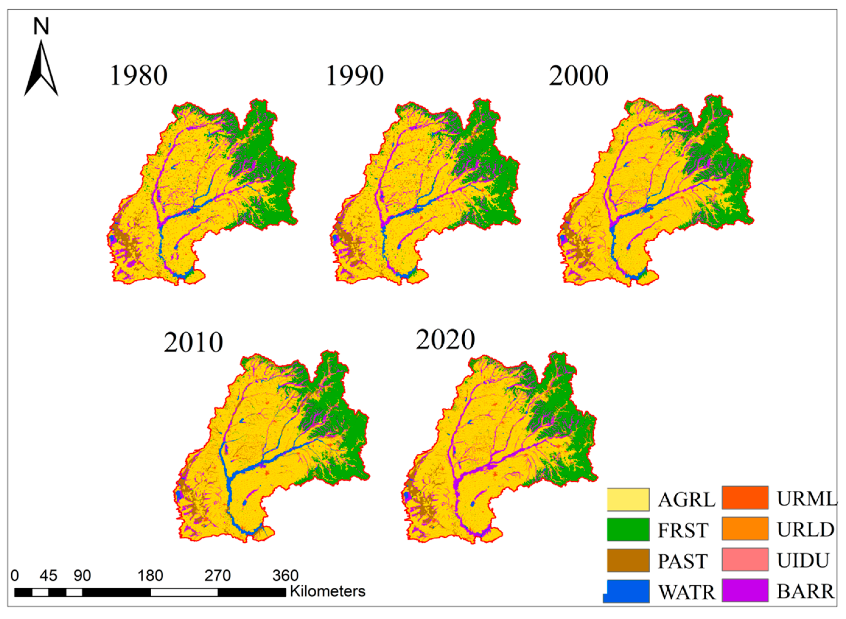
3.1. Land Use Change Analysis

The analysis quantitatively examined the area and distribution of different land use types within Hulan River Basin using ArcGIS 10.6 (

Table 6. Different historical land use area ratios.

Land Use Type	1980		1990		2000		2010		2020
	Area (km2)	Percent (%)	Area (km2)	Percent (%)	Area (km2)	Percent (%)	Area (km2)	Percent (%)	Area (km2)	Percent (%)
AGRL	21,396.34	0.57	21,634.47	0.58	22,499.56	0.60	22105	0.59	22435	0.60
FRST	8774.81	0.23	8646.80	0.23	7846.85	0.21	8014.55	0.21	7766.47	0.21
PAST	1716.85	0.05	1669.26	0.04	1738.09	0.05	2216.57	0.06	1857.66	0.05
WATR	870.90	0.02	842.62	0.02	872.16	0.02	1421.72	0.04	1517.00	0.01
URML	119.71	0.00	135.78	0.00	151.10	0.00	185.64	0.00	179.32	0.00
URLD	1071.41	0.03	1122.16	0.03	1117.61	0.03	1249.19	0.03	1120.17	0.03
UIDU	3.99	0.00	2.00	0.00	3.08	0.00	14.88	0.00	37.66	0.00
BARR	3594.32	0.10	3495.26	0.09	3319.89	0.09	2340.78	0.06	2635.00	0.10

). The results suggest significant alterations in land utilization within the basin. Cultivated land and forest land are the predominant types of land, comprising more than 60% and 20% of the total area, respectively. Over the period spanning from 1980 to 2020, there has been a consistent upward trend in cultivated land, compared with a declining trend in forest land. The alterations can be ascribed to the focus on agricultural cultivation and governmental initiatives that advocate for holistic agricultural advancement in Hulan River Basin. The amount of fallow land has consistently diminished, whereas the utilization of urban land has exhibited a steady upward trajectory. The observed trends could potentially be linked to agricultural reclamation and urban expansion activities taking place within Hulan River Basin.

Through the utilization of the land transfer matrix, an analysis was conducted to investigate changes in land use area within Hulan River Basin. This approach enables a quantitative assessment of the direction and extent of land use transition across various land categories. To represent the transition characteristics among various land use types, the results of the transfer matrix were illustrated through a chord diagram (

Table 7. Land use changes and dynamics within study area (1980–2020).

Land Use Type	1980–1990		1990–2000		2000–2010		2010–2020		1980–2020
	Area Change (km2)	Single LUD Index (%)	Area Change (km2)	Single LUD Index (%)	Area Change (km2)	Single LUD Index (%)	Area Change (km2)	Single LUD Index (%)	Area Change (km2)	Single LUD Index (%)
AGRL	238.13	0.11	865.08	0.40	−394.56	−0.18	330.06	0.15	1038.72	0.49
FRST	−128.01	−0.15	−799.95	−0.93	167.70	0.21	−248.08	−0.31	−1008.4	−1.15
PAST	−47.60	−0.28	68.83	0.41	478.48	2.75	−358.91	−1.62	140.81	0.82
WATR	−28.28	−0.32	29.54	0.35	549.57	6.30	95.28	−7.97	646.10	−6.68
URML	16.07	1.34	15.33	1.13	34.54	2.29	−6.32	−0.34	59.61	4.98
URLD	50.74	0.47	−4.55	−0.04	131.58	1.18	−129.03	−1.03	48.75	0.46
UIDU	−1.99	−5.00	1.09	5.44	11.80	38.27	22.78	15.31	33.67	84.38
BARR	−99.06	−0.28	−175.37	−0.50	−979.11	−2.95	294.22	6.50	−959.32	0.75
CLUD Index (%)	0.08		0.26		0.37		0.20		0.52

) and an LUD change diagram (Figure 4). A detailed examination of these diagrams indicates that the most significant land use conversion occurred between 2000 and 2010, with a subsequent period of relative stability. Over a period of 40 years, there was an increase of 1038 km² in the area of arable land, accompanied by a reduction of 1008 km² in forested land, and a decrease of 959 km² in unused land. The conversion of forested land, unused land, and grassland into arable land amounted to 969 km², 911 km², and 566 km², respectively. The changes in land use patterns in Hulan River Basin are significant, highlighting the importance of incorporating historical land use data in the selection of a natural runoff model [47].

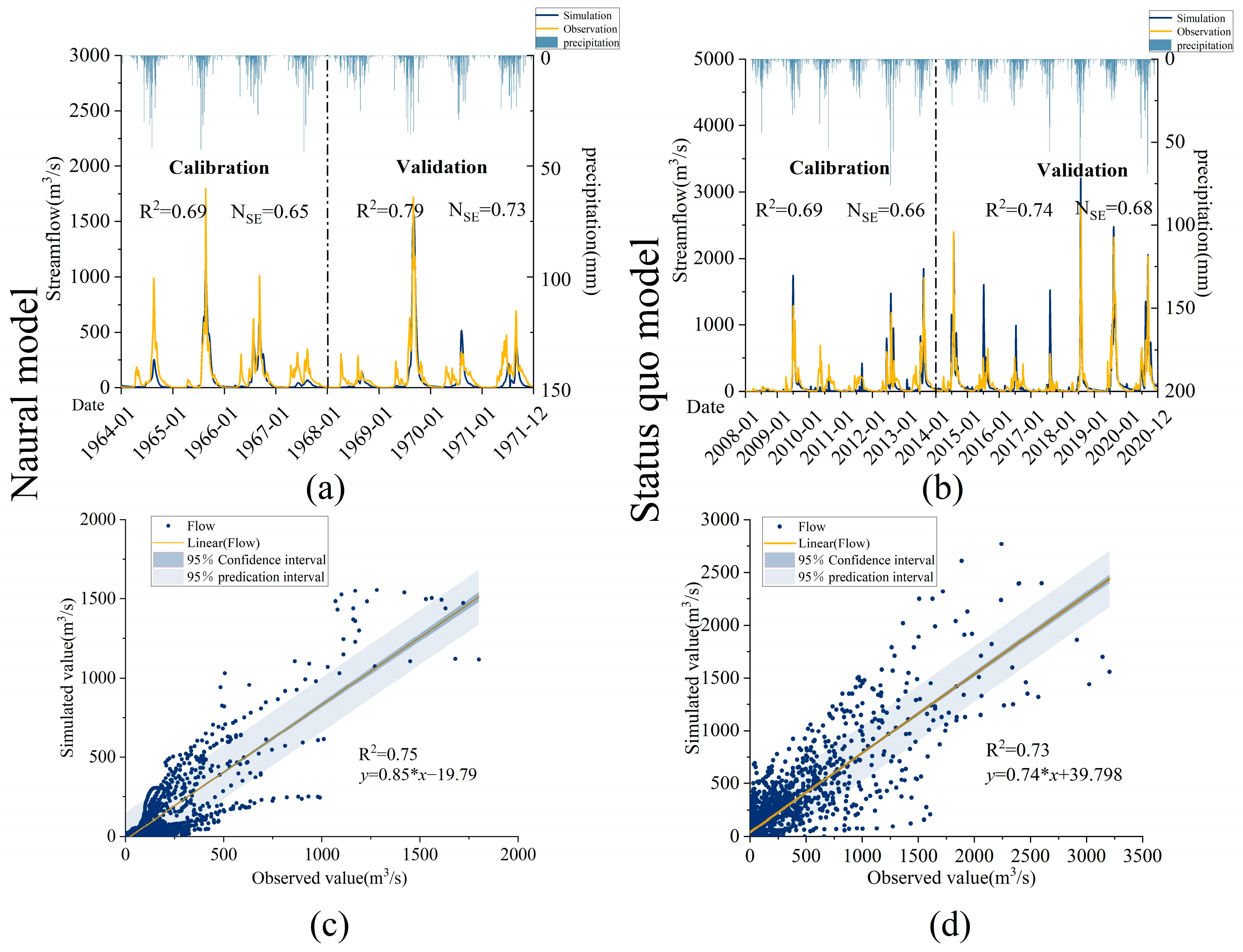
3.2. Results of Runoff Simulation and Watershed Division

In the runoff simulation process, this study identified 28 parameters by referring to previous research results and following SWAT operational guidelines [48,49]. The selected parameters and their meanings are shown in

Table 8. SWAT model parameter descriptions.

Parameter	Description	Parameter	Description
SOL_Z	Soil layer depth from surface to bottom	SFTMP	Snowfall temperature
CH_N2	Manning’s “n” value for main flow channel	EPCO	Plant uptake compensation factor
BIOMIX	Biological mixing efficiency	ESCO	Soil evaporation compensation factor
TLAPS	Temperature lapse rate	CANMX	Maximum canopy storage
GWQMN	Minimum aquifer depth for groundwater return flow	HRU_SLP	Average slope steepness multiplicative factor
GW_DELAY	Groundwater delay time	SLSUBBSN	Average slope length multiplicative factor
ALPHA_BF	Baseflow alpha factor	ALPHA_BNK	Alpha factor for bank storage baseflow
CN2	SCS-CN for moisture condition II	SOL_ALB	Moist soil albedo multiplicative factor
SNOCOVMX	Threshold depth of snow at 100% coverage	SOL_K	Soil hydraulic conductivity
SURLAG	Surface runoff lag coefficient	RCHRG_DP	Deep aquifer percolation fraction
TIMP	Snow pack temperature lag factor	SOL_AWC	Soil available water capacity
SMFMN	Maximum snowmelt factor for December 21	CH_K2	Effective hydraulic conductivity in main channel alluvium
SMFMX	Maximum snowmelt factor for June 21	REVAPMN	Threshold depth of water in shallow aquifer required to allow re-evaporation to occur
SMTMP	Snowmelt base temperature	GW_REVAP	Groundwater re-evaporation coefficient

. SWAT-CUP was employed for parameter calibration [50]. In this study, a sensitivity analysis of SWAT parameters was carried out utilizing the Sequential Uncertainty Fitting (SUFI-2) algorithm due to the extensive number of SWAT parameters [51,52]. The overall R² was 0.75 (Figure 5). In the context of the status quo runoff, R² values for the calibration and validation periods were 0.69 and 0.74, respectively, resulting in an overall R² of 0.73. These values suggest that the calibrated SWAT model exhibits a certain degree of relevance to Hulan River Basin [53,54]. Figure 6 illustrates the bubble chart depicting the sensitivity of the SWAT model parameters. The sensitivity of the parameters was assessed using the t-Stat value and p value. A larger absolute value of t indicates increased sensitivity, whereas a p value closer to 0 indicates greater statistical significance. The chart indicates that CH_N2 exhibits the highest level of sensitivity among the parameters analyzed. In addition to CH_N2, maximum canopy interception (CANMX), initial SCS runoff curve number (CN2), and base flow ALPHA factor significantly impact runoff simulation in Hulan River Basin. The 28 sensitive parameters were readopted into the SWAT model for parameter refinement and recalibration. Manual adjustments were made according to the simulation results to improve the accuracy of the model. R² values for the calibration and validation periods of the natural runoff model were 0.69 and 0.79, respectively. The simulated outcomes for the status quo runoff during both the calibration and validation periods are illustrated in Figure 6. Furthermore, the flow data from 1990 to 2020 was classified into wet and dry periods by applying CAM within the framework of the natural runoff model (Figure 7). The average and index curves of cumulative anomaly for the monthly average flow in Hulan River Basin demonstrate a rising trend from June to October and a declining trend from November to May. This pattern indicates that the flood season in Hulan River Basin transpires from June to October annually, while the non-flood season takes place from November to May of the subsequent year.

The validity of the natural model of SWAT was confirmed through detailed sub-item analysis, with the results illustrated in Figure 8. The results indicate that R² for the simulated runoff values in Hulan River Basin reached 0.73, suggesting a high level of validity in the construction of the natural model. The simulation performance was superior during the wet years compared to dry and normal years. The most optimal simulation years were 1962 and 1963, while the least optimal were 1980 and 1990.

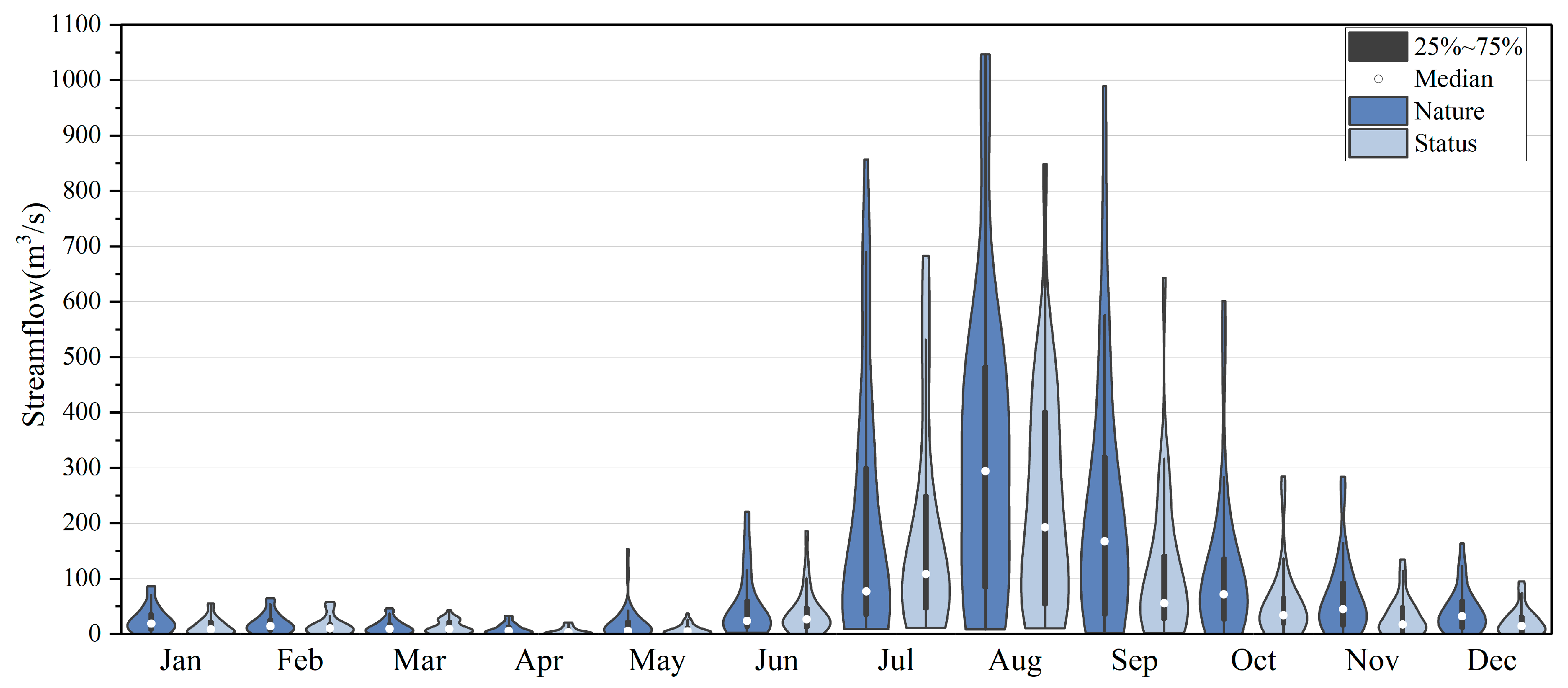
3.3. Runoff Status Assessment

To delve deeper into the impact of human activities on the hydrological conditions of Hulan River Basin, the runoff data generated by the SWAT natural runoff model in Hulan River Basin from 1962 to 2020 were categorized into wet and dry years using the standardized anomaly percentage outlined in the hydrological information forecast specification (GB/T 22482-2008). The years characterized by wet conditions (2012–2020), average precipitation levels (2009, 2010), and dry weather patterns (2008, 2011) were sequentially identified.

The disparate allocation of hydrological components within the basin varies significantly between the flood season and non-flood season, primarily impacted by climatic conditions. Analysis of the daily scale simulation results of the natural model and the status quo model (Figure 9) indicates that human water consumption constitutes around 40% of the surface water resources, while the status quo runoff of Hulan River accounts for approximately 60% of the natural runoff. According to the “Calculation Specification for Water Demand of River and Lake Ecological Environment” (SL/T 712-2021), the surface water resources of Hulan River are undergoing moderate development and utilization. With the exception of July, the median natural runoff surpasses that of the status quo runoff. Approximately 85% of the total annual runoff transpires during the flood season (June–October), suggesting that precipitation plays a pivotal role as the primary influencing factor for Hulan River Basin.

Figure 10 depicts alterations in the spatial distribution and proportion of basin runoff due to human activities, leading to a decrease in runoff for each sub-basin. The greatest declines are observed in May (non-flood season) at roughly 64% and in October (flood season) at approximately 54%. On average, reductions are 46% during the non-flood season and 36% during the flood season. Consequently, water consumption in the Hulan River Basin is considered moderate.

3.4. The Optimization of the Ecological Flow Calculation

Based on the simulated values of the SWAT natural runoff model in Hulan River Basin from 1990 to 2020, various methodologies were employed to calculate the ecological flow at Lanxi station section of Hulan River Basin. The calculations’ outcomes are displayed in

Table 9. Results of ecological flow estimated across different methods.

Method	Month
	1	2	3	4	5	6	7	8	9	10	11	12
Distribution	3.32	2.53	1.71	1.39	2.97	6.91	27.6	46.	5.05	3.34	8.37	5.39
Monthly Minimum	2.22	1.39	0.41	1.67	2.98	10.1	28.4	38.7	17.7	9.38	5.19	3.94
Texas	7.65	6.05	4.08	2.06	2.68	8.85	28.9	92.4	51.4	22.4	14.3	10.3
Q50	25.5	20.2	13.6	6.87	8.92	29.5	96.3	308	171	75	47.6	34.2
Q75	12.6	10	5.99	2.80	4.69	13.6	33.5	87.4	39	33.4	19.1	13.7
Q90	4.62	5.02	2.66	1.80	2.56	7.83	26.1	46.6	32.	21.2	13.7	9.89
Tessman	28.3	21.2	14.5	11.2	23.2	39.2	83.3	138	94.7	48	39.2	39.2
DFM (Q0)	16.5	11.4	7.63	4.78	8.36	20.7	65.8	259	113	63.3	35.6	24.7
DFM (Q1)	19.2	14	9.55	6.53	12	43.7	138	428	156	91.7	44.1	26.9
DFM (Q2)	14.2	9.68	5.47	2.14	3.03	7.65	26.5	97	74	45	27.2	20.8
DFM (Q3)	17.8	12.7	8.59	5.66	10.2	32.2	102	343	135	77.5	39.8	25.8
DFM (Q4)	15.3	10.6	6.55	3.46	5.69	14.2	46.2	178	93	54.2	31.4	22.7
DFM (Q5)	99.5	71.4	53	37.5	329	530	1208	1421	1251	846	430.	199
DFM (Q6)	0.00	0.00	0.00	0.00	0.00	0.00	1.02	2.07	0.00	0.00	0.00	0.00
NGPRP	24.7	18.8	12.4	9.63	23.7	46.8	231	295	200	111	62.1	35.9
Tennant (Excellent)	17	12.7	8.67	6.70	13.9	31.9	125	207	142	80	41.5	26.6
Tennant (Very Good)	8.5	6.37	4.34	3.35	6.95	26.6	104	172	118	60	20.8	13.3
Tennant (Good)	5.67	4.25	2.89	2.23	4.64	21.3	83	138	95	48	13.8	8.87
Tennant (Medium)	2.83	2	1.45	1.12	2.32	15.9	62.5	103	71	36	6.92	4.43
Tennant (Bad)	2.83	2	1.45	1.12	2.32	5.31	20.8	34	24	12	6.92	4.43

. The minimum ecological flow threshold and the most suitable ecological flow threshold are the primary methods utilized in the calculation of ecological flow. Consequently, this study focuses on individually examining these two thresholds.

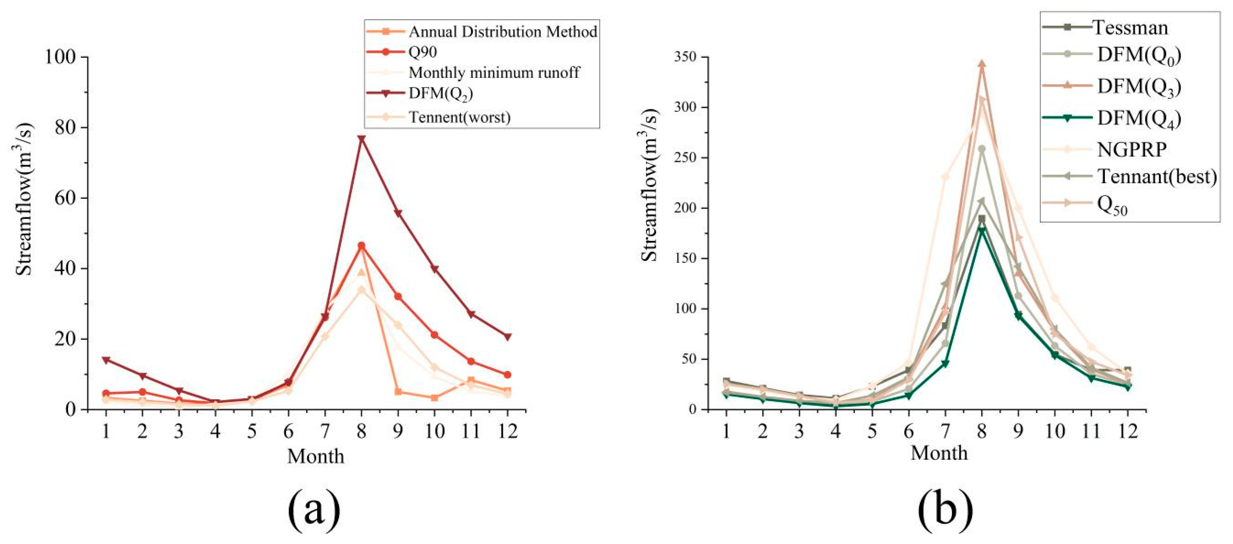
3.4.1. Calculation Method Selection of Minimum Ecological Flow

In this study, multiple methodologies were utilized to establish the minimum ecological flow threshold. These methods included the variable Q₉₀ method, the annual distribution method, the monthly minimum value method, DFM (Q₂) method, and Tennant method. The outcomes of the ecological flow calculations are illustrated in Figure 10. According to “Calculation Specification for Ecological Water Demand in Rivers and Lakes” (SL/T 712-2021), it is advisable to uphold the fundamental ecological flow in moderately developed small- and medium-sized rivers at a level of 10% or higher (as per Tennant method difference level). However, the annual distribution method and the monthly minimum value method occasionally fail to meet the threshold set by the Tennant method in specific months. Therefore, these methods are not suitable for calculating the minimum ecological flow of Hulan River.

Both the Q₉₀ variable method and DFM (Q₂) method satisfy the 10% exceedance flow criterion for natural river flow. Ecological flow should not only satisfy water demands at different time intervals but also preserve the seasonal fluctuation pattern of river flow, known as hydrological rhythm. In this study, a correlation analysis was performed to examine the relationship between the Q₉₀ method variable and DFM (Q₂) method in relation to natural flow processes. The results indicated a correlation coefficient of 0.99 between the Q₉₀ method and natural flow, and a correlation coefficient of 0.93 between the DFM (Q₂) method and natural flow. Therefore, the Q₉₀ variable method was chosen to compute the minimum ecological flow process for the entire basin (Figure 11).

Figure 12 demonstrates the spatial characteristics of the ecological flow in Hulan River, indicating a significantly higher ecological flow requirement in the main downstream channel compared to its tributaries. The peak demand for ecological flow is observed in August, whereas the lowest demand occurs in April.

3.4.2. Calculation Method Selection of Maximum Ecological Flow

In this study, a comprehensive evaluation of different approaches for determining ecological flow in Hulan River was undertaken. The methods evaluated included the Texas method, Q₅₀ method, Tessman method, DFM, and Tennant method. The results (Figure 11) indicate that the variations in the computed results across the six methods are not statistically significant. However, it is noteworthy that only DFM provides upper and lower thresholds for determining the most appropriate ecological flow. The values obtained from various methods generally align with the upper and lower thresholds established by DFM. Previous research frequently establishes the upper and lower thresholds for the optimal ecological flow by either adding or subtracting standard deviations from the mean ecological flow, or by employing envelope curves derived from various hydrological methodologies. However, these methods are vulnerable to significant runoff extremes. DFM, in contrast, is based on probability density functions and has the capability to reduce the impact of extreme values on ecological flow computations. Consequently, DFM was chosen in this study to calculate the most appropriate ecological flow in Hulan River.

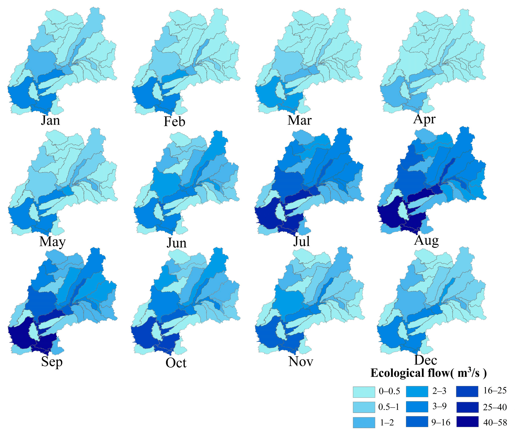
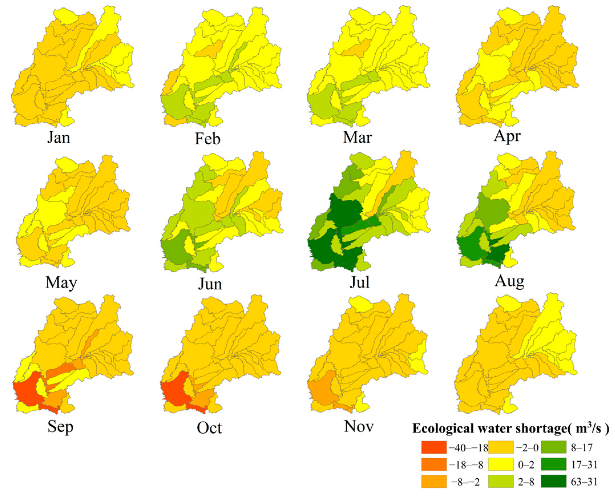
3.5. Quantification of Ecological Water Replenishment

Ecological water replenishment pertains to the deliberate augmentation of water levels to fulfill the prescribed ecological flow criteria of river channels. The ecological flow target chosen for this study represents the most appropriate ecological flow determined through DFM. In Figure 13, prevalent water scarcity is observed in the basin throughout the year, except for the months of June, July, and August. However, the discrepancy between the majority of time intervals and the optimal ecological flow is not substantial. Extreme water scarcity occurrences are infrequent, and it is possible to sustain a monthly water replenishment volume below 2 × 10⁷ m³. During September and October, ecological water deficits are prevalent in the majority of sub-basins, leading to significant water scarcity in the downstream main stream. It is crucial to explore external water diversion techniques as a means to augment the water flow within the river channel, thereby safeguarding the well-being of aquatic flora and fauna. The peak ecological satisfaction level occurs in March with the exception of sub-basin four, which necessitates ecological water replenishment.

4. Discussion

4.1. Land Use Transfer Analysis

In this study, a quantitative analysis of land use change and transfer in Hulan River Basin was undertaken through the computation of both the single dynamic change degree and the comprehensive dynamic change degree. The most notable land use transformation in Hulan River Basin took place between 2000 and 2010, characterized by a substantial expansion of arable land and a pronounced reduction in forested areas. These results align with the land use change analysis results in the northeast region conducted by Wang et al. [55].

Furthermore, the comparison between the natural and status quo daily runoff models indicated that alterations in land use have a discernible effect on the development of SWAT’s daily runoff model. The decrease in forest and grassland areas contributes to intensified runoff levels during flood seasons. Conversely, the expansion of impermeable surfaces like urban and industrial areas hinders rainfall infiltration, leading to escalated surface runoff. These results align with the research results of Li et al. [56] concerning Weihe River and Liu et al. [57] regarding Xihe River.

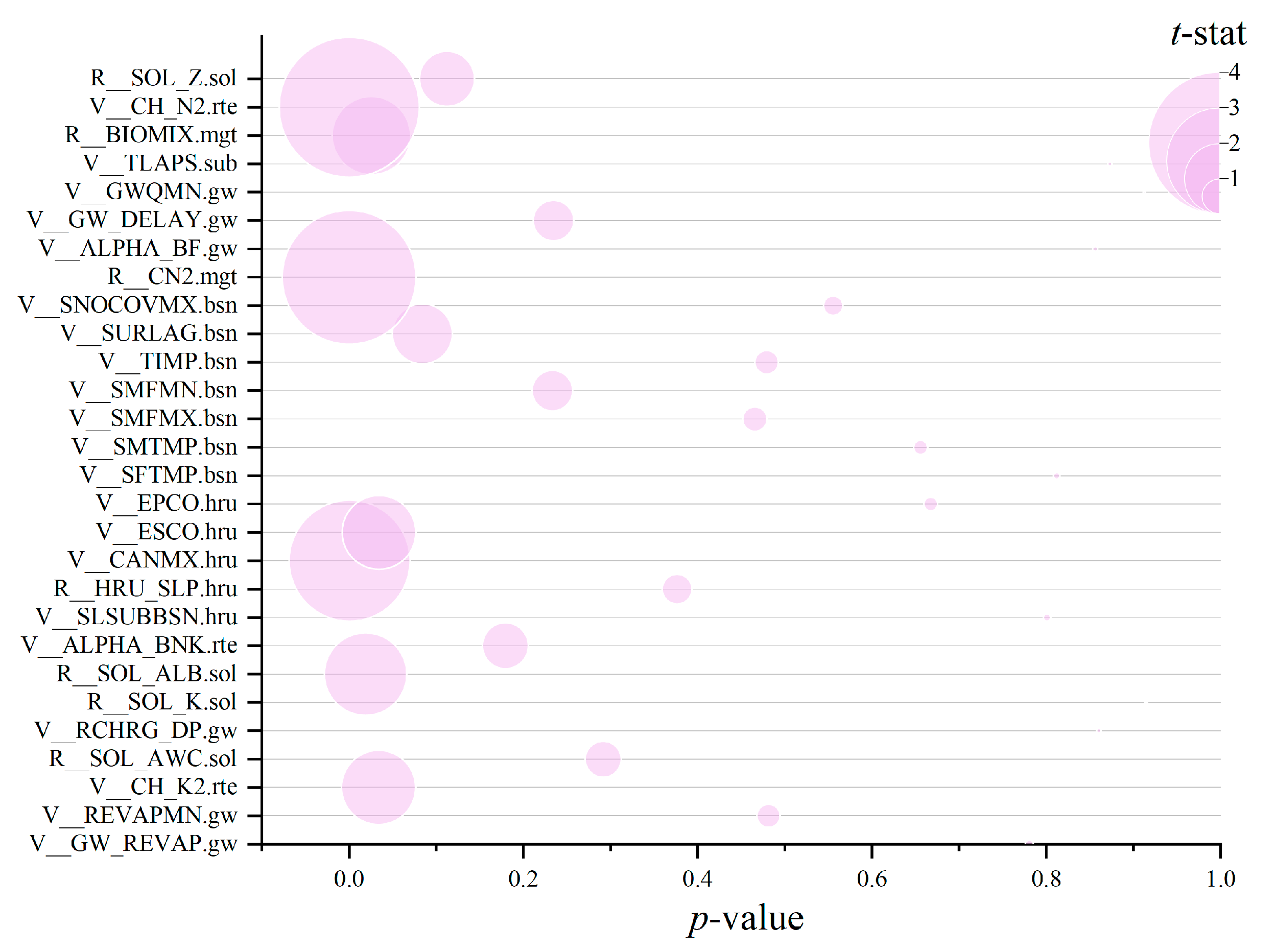
4.2. SWAT Model Building and Parameter Sensitivity Analysis

This study utilized SWAT to delineate the sub-watersheds within Hulan River Basin. Lanxi station section (sub-watershed No. 29) was determined to possess a watershed area of 27,720 km², which aligns with the value of 27,736 km² [58] documented in the hydrological yearbook. By implementing the SWAT model for Hulan River Basin and performing an assessment of the current runoff situation, this study concluded that the level of surface water development in the basin is estimated to be around 40%. Precipitation was recognized as a principal factor affecting runoff in Hulan River, aligning with prior research results [59,60]. However, insufficient attention to snowmelt runoff led to inadequate simulation of spring runoff in the basin.

Previous studies have examined the sensitivity of parameters in Hulan River Basin in relation to parameter sensitivity analysis [22,61,62,63]. Variations in t-Stat values, p value values, and sensitivity rankings across studies were ascribed to differences in the iteration times of SWAT-CUP and the choice of running program algorithms. However, CH_N2, the maximum canopy interception CANMX, the initial SCS runoff curve number CN2, the groundwater delay coefficient GW_DELAY, and the base flow ALPHA factor were recognized as sensitive parameters in various studies.

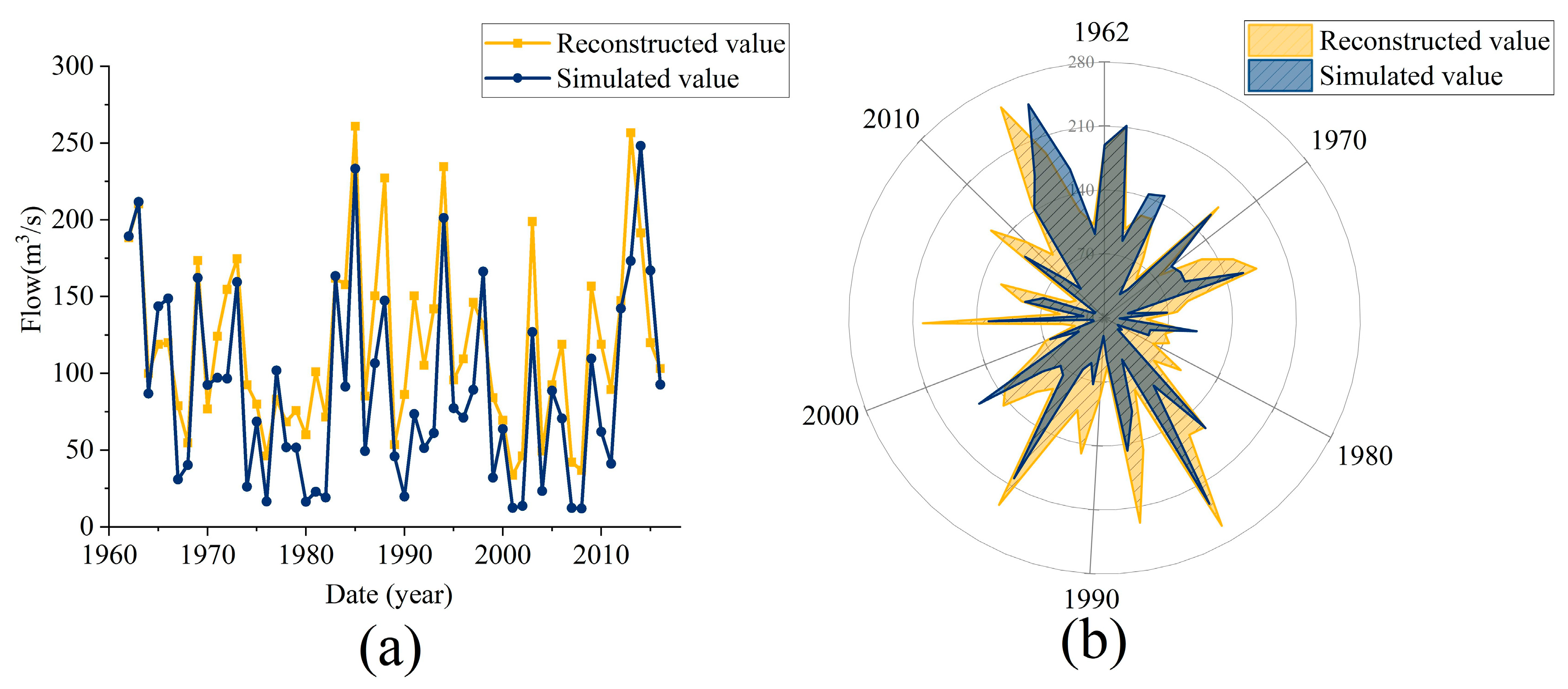
4.3. Natural Flow Restoration

For natural flow restoration, previous research has predominantly employed a fragmented research methodology to enhance natural flow by incorporating human water activities into empirical hydrological data. These activities include inter-basin water transfer projects, reservoirs, water intake projects, and irrigation projects [18,21,64,65,66,67]. Numerous studies have alternatively integrated partial investigations with distributed hydrological models to reestablish the natural flow within the basin [68,69,70]. However, the partial investigation method is found to be impractical for ecological flow calculations that require daily natural flow data. Therefore, this study employs a methodology that entails selecting flow measurements from a period characterized by minimal human impact to develop a natural model of the basin. Subsequently, the partial investigation method is utilized to reconstruct the annual natural flow and validate the model. This approach not only guarantees the accuracy of the natural model but also reduces the workload associated with daily restoration of natural flow.

4.4. Ecological Water Requirement Calculation

In previous studies, the selection of methods for calculating ecological flow has frequently concentrated on determining ecological flow or ecological water demand either at the outlet of the watershed or at a specific section of the main river channel [71,72]. However, this approach has failed to consider the spatial and temporal variations in water scarcity throughout the entire watershed. Therefore, this study assessed ecological water scarcity in Hulan River Basin by comparing natural runoff models with status quo runoff models. This approach enables a more thorough examination of the hydraulic connectivity among sub-watersheds, promoting a holistic strategy for ecological restoration through the integration of point and surface sources, upper and lower watershed connections, and the coordination of multiple objectives.

Prior research has extensively explored hydrological calculation methods for determining ecological flow [24,73,74]. In this study, a hybrid approach utilizing natural runoff models and diverse hydrological methodologies was implemented for computation purposes. The magnitude of ecological flow determined by the chosen hydrological method closely aligns with the optimal ecological flow calculated by Jing et al. [23] using River-2D for the Tieling section of Hulan River. This consistency underscores the dependability of the natural runoff model employed in this study and the efficacy of DFM in ecological flow calculations. However, in DFM, this study chose to utilize Gaussian kernel function for the probability density function. However, it is crucial to acknowledge that the distribution of flow varies among different watersheds [75]. Therefore, Gaussian kernel function may not be the most appropriate choice for Hulan River Basin. Future studies should conduct a comparative analysis of the goodness of fit of different probability density functions to hydrological data within Hulan River Basin to ascertain the most suitable probability density function.

4.5. Methods Advantages and Limitations

In the context of runoff simulation, this study employs the SWAT model for runoff simulation. The SWAT model has been extensively utilized on a global scale, and contemporary research on the SWAT model is considered well developed. However, numerous facets of the SWAT model necessitate enhancement and fine-tuning. For instance, the accuracy of simulating groundwater processes in the SWAT model is constrained due to its utilization of simplistic linear functions for groundwater process simulation. This constraint impedes the SWAT model’s capacity to accurately replicate watersheds characterized by substantial groundwater extraction and frequent interactions between groundwater and surface water. In forthcoming research, the amalgamation of SWAT model with other models has the potential to improve the precision of simulations.

The utilization of DFM, incorporating kernel density functions in lieu of conventional frequency density functions, mitigated the impact of extreme flow values on ecological flow computations. This adaptation renders DFM more appropriate for cold regions and seasonal rivers. A comparison of DFM with other hydrological approaches indicates that the optimal ecological flow determined through DFM represents a threshold rather than a precise value. This characteristic enhances the feasibility of ecological water replenishment. The majority of hydrological methods chosen for this study produce ecological flow values that fall within the range of optimal ecological flow values determined by DFM, thus affirming its scientific validity. However, similar to many academic inquiries, this study is not devoid of limitations, including the ambiguity surrounding the selection of kernel functions in DFM. The Gaussian kernel function employed in this research is commonly used, however, it may not be the most appropriate choice for Hulan River Basin. Future research may entail the comparison of different kernel functions with river runoff processes to determine the most suitable one for the specific region, prior to its application in calculating ecological flows through DFM.

5. Conclusions

This study provides a quantitative assessment of land use changes in Hulan River Basin by analyzing the LUD index and land use change matrix. Furthermore, the evaluation of the ecological water deficit in Hulan River Basin involves the development of natural runoff models and status quo runoff models, as well as the application of diverse hydrological techniques. The primary results derived from this investigation can be summarized as follows:

• The land use change observed in Hulan River Basin between 2000 and 2010 demonstrated a significant transformation, highlighted by an increase in arable land and a considerable decrease in forested areas.
• In the evaluation of the minimum ecological flow, DFM yields slightly higher results in comparison to other methodologies. While both the variable Q₉₀ method and DFM (Q₂) method achieve a 10% match with the natural river flow, DFM exhibits a marginally lower level of adherence to hydrological patterns compared to the variable Q₉₀ method.
• In the assessment of the optimal ecological flow for Hulan River Basin, it has been noted that different hydrological approaches produce comparable outcomes. However, only DFM has the capability to quantify the threshold of the optimal ecological flow. Furthermore, it is worth noting that the majority of results derived from alternative hydrological methods align with this threshold. Therefore, it is considered more suitable to utilize DFM for determining the ecological flow of Hulan River Basin.
• The utilization of the SWAT model to simulate the natural runoff dynamics of Hulan River has demonstrated a significant decrease in the resources needed for reinstating natural runoff, in contrast to traditional approaches to allocation and restoration. This approach involves reduced and simplified data requirements, yet it is also able to fulfill the stringent requirements set by DFM for hydrological data.
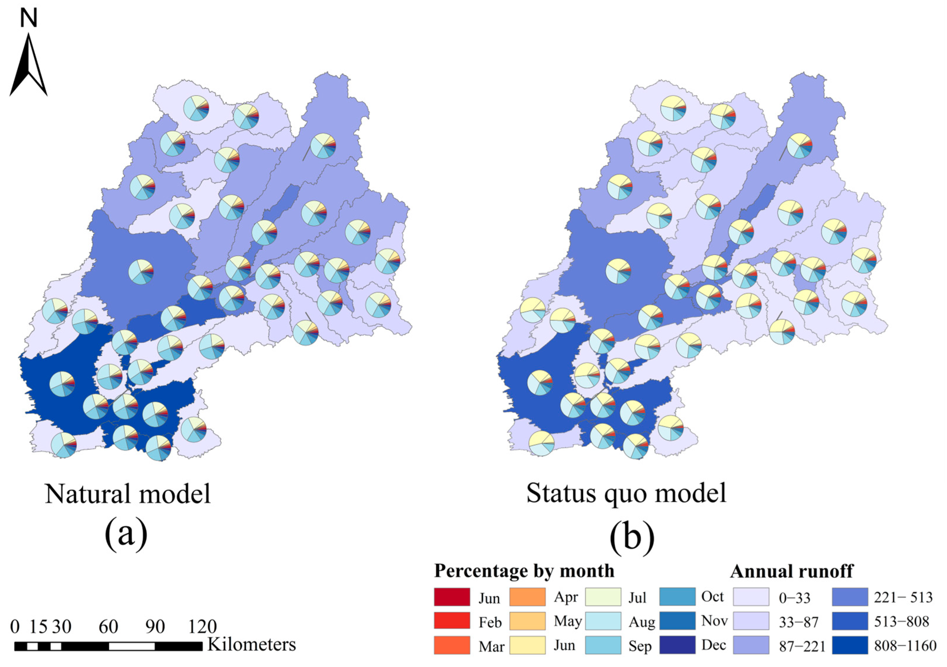
• The SWAT model is utilized to evaluate ecological flow and ecological water scarcity throughout the watershed, taking into account the hydraulic interconnections among sub-watersheds. This methodology enables the assessment of the spatiotemporal distribution of ecological flow and water scarcity in the watershed. Consequently, it facilitates a more intuitive and rational spatial allocation of water resources to fulfill the overarching ecological flow requirements.

References

1. Wu, M.; Chen, A.; Zhang, X.N.; McClain, M.E. A Comment on Chinese Policies to Avoid Negative Impacts on River Ecosystems by Hydropower Projects. Water 2020, 12, 869. [Google Scholar] [CrossRef]
2. Wang, Y.; Li, X.M.; Zhang, F.; Wang, W.W.; Xiao, R.B. Effects of Rapid Urbanization on Ecological Functional Vulnerability of the Land System in Wuhan, China: A Flow and Stock Perspective. J. Clean. Prod. 2020, 248, 119284. [Google Scholar] [CrossRef]
3. Wang, F.Y.; Tong, S.; Chu, Y.; Liu, T.L.; Ji, X. Spatio-Temporal Evolution of Key Areas of Territorial Ecological Restoration in Resource-Exhausted Cities: A Case Study of Jiawang District, China. Land 2023, 12, 1733. [Google Scholar] [CrossRef]
4. Li, Z.; Huang, B.; Qiu, J.; I, Y.; Yang, Z.; Chen, S. Analysis on evolution characteristics of ecological flow of Hanjiang River under changing environment. Water Resour. Prot. 2021, 37, 22–29. [Google Scholar]
5. Li, Y.; Sun, C.; Liu, H. Supervision of river ecological flow and verification of control objectives in Fujian Province. Water Resour. Prot. 2020, 36, 92–96+104. [Google Scholar]
6. Huang, S.Z.; Chang, J.X.; Huang, Q.; Wang, Y.M.; Chen, Y.T. Calculation of the Instream Ecological Flow of the Wei River Based on Hydrological Variation. J. Appl. Math. 2014, 2014, 127067. [Google Scholar] [CrossRef]
7. SL/T 712-2021; Specification for Calculation of Ecological Flow for Rivers and Lakes. 2021. Available online: https://www.nssi.org.cn/nssi/front/114226640.html (accessed on 11 March 2024).
8. Tang, Q.C. Water resources and oasis construction in Tarim Basin. Resour. Sci. 1989, 6, 28–34. [Google Scholar]
9. Meng, Y.; Xu, W.J.; Guan, X.J.; Guo, M.; Wang, X.R.; Yan, D.H. Ecology-Habitat-Flow Modular Simulation Model for the Recommendation of River Ecological Flow Combination. Environ. Model. Softw. 2023, 169, 105823. [Google Scholar] [CrossRef]
10. Zheng, Y.W.; Yang, T.; Wang, N.; Wan, X.H.; Hu, C.T.; Sun, L.K.; Yan, X.R. Quantifying Hydrological-Ecological Response Relationships Based on Zooplankton Index of Biotic Integrity and Comprehensive Habitat Quality Index—A Case Study of Typical Rivers in Xi’an, China. Sci. Total Environ. 2023, 858, 159925. [Google Scholar] [CrossRef]
11. Wang, B.; Cheng, H.; He, X.J.; Xu, Y.P.; Guo, Y.X.; Geng, F.; Wang, C. Study on Early Warning and Forecasting Model of Ecological Flow in Rivers and Lakes Based on LSTM Deep Learning. J. China Hydrol. 2023, 43, 65–70. [Google Scholar]
12. Tian, X.R.; Jiang, N.; Shi, Q.; Li, D.L.; Ni, P.; Liu, Y.; Wang, X.X. Study on River Ecological Flow Based on Improved Annual Distribution Method. Water Sav. Irrig. 2022, 10, 31–36. [Google Scholar]
13. Yu, S.; He, L.; Lu, H.W. A Tempo-Spatial-Distributed Multi-Objective Decision-Making Model for Ecological Restoration Management of Water-Deficient Rivers. J. Hydrol. 2016, 542, 860–874. [Google Scholar] [CrossRef]
14. Yu, S.; Wang, M.Y. Comprehensive Evaluation of Scenario Schemes for Multi-Objective Decision-Making in River Ecological Restoration by Artificially Recharging River. Water Resour. Manag. 2014, 28, 5555–5571. [Google Scholar] [CrossRef]
15. Kal, B.-S.; Cho, S.-H.; Park, C.-D.; Mun, H.-S.; Joo, Y.-E.; Park, J.-B. Watershed Water Quality Management Plan Using Swat and Load Duration Curve. J. Korean Assoc. Geogr. Inf. Stud. 2021, 24, 41–57. [Google Scholar]
16. Liu, Y.; Li, H.Y.; Cui, G.; Cao, Y.Q. Water Quality Attribution and Simulation of Non-Point Source Pollution Load Flux in the Hulan River Basin. Sci. Rep. 2020, 10, 1941. [Google Scholar] [CrossRef]
17. Cui, G.N.; Bai, X.Y.; Wang, P.F.; Wang, H.T.; Wang, S.Y.; Dong, L.M. Agricultural Structures Management Based on Nonpoint Source Pollution Control in Typical Fuel Ethanol Raw Material Planting Area. Sustainability 2022, 14, 7995. [Google Scholar] [CrossRef]
18. Niu, Z.R.; Wang, Q.Y.; Sun, D.Y.; Zhang, R.; Wu, X.; Xing, Y.P.; Zhan, S.J. Runoff variation characteristics of Taohe River Basin based on calculation of current runoff. Arid Land Geogr. 2021, 44, 149–157. [Google Scholar]
19. Yang, R.; Feng, M.Q.; Sun, X.P.; Yang, Z. Calculation Method of Environmental Flow in the Middle Reaches of Fenhe River Based on Improved Tennant Method. Water Resour. Power 2018, 36, 13–15. [Google Scholar]
20. Wang, Y.X.; Hu, T.S.; Wang, J.L.; Wu, F.Y.; Wang, X. Approach for water resources assessment based on runoff component investigation method and SWAT model. J. Water Resour. Water Eng. 2023, 34, 54–65. [Google Scholar]
21. Jia, S.F.; Liang, Y.; Zhang, S.F. Discussion on evaluation of natural runoff in the Yellow River Basin. Water Resour. Prot. 2022, 38, 33–38+55. [Google Scholar]
22. Liu, Y.; Cui, G.; Li, H.Y. Optimization and Application of Snow Melting Modules in Swat Model for the Alpine Regions of Northern China. Water 2020, 12, 636. [Google Scholar] [CrossRef]
23. Jing, M.Y.; Wang, L.Q.; Chu, L.L.; Li, T.N. Research on the Ecological Flow of the Mainstream of the Hulan River Based on the Improved River2D Model. China Rural Water Hydropower 2023, 3, 102–110+119. [Google Scholar]
24. Wu, M.; Chen, A. Practice on Ecological Flow and Adaptive Management of Hydropower Engineering Projects in China from 2001 to 2015. Water Policy 2018, 20, 336–354. [Google Scholar] [CrossRef]
25. Ridwansyah, I.; Yulianti, M.; Apip; Onodera, S.-I.; Shimizu, Y.; Wibowo, H.; Fakhrudin, M. The Impact of Land Use and Climate Change on Surface Runoff and Groundwater in Cimanuk Watershed, Indonesia. Limnology 2020, 21, 487–498. [Google Scholar] [CrossRef]
26. Eeshan, K.T.; Saraswat, D.; Singh, G. Comparative Analysis of Bioenergy Crop Impacts on Water Quality Using Static and Dynamic Land Use Change Modeling Approach. Water 2020, 12, 410. [Google Scholar]
27. Naikoo, M.A.; Ahanger, M.A. Land Use/Land Cover Change Detection and Validation of Swat Model on Vishow Sub-Basin Using Remote Sensing and Gis Techniques. Int. J. Hydrol. Sci. Technol. 2022, 13, 43–56. [Google Scholar] [CrossRef]
28. Nkwasa, A.; Chawanda, C.J.; Msigwa, A.; Komakech, H.C.; Verbeiren, B.; van Griensven, A. How Can We Represent Seasonal Land Use Dynamics in Swat and Swat Plus Models for African Cultivated Catchments? Water 2020, 12, 1541. [Google Scholar] [CrossRef]
29. Liu, Y.G.; Xu, Y.X.; Zhao, Y.Q.; Long, Y. Using Swat Model to Assess the Impacts of Land Use and Climate Changes on Flood in the Upper Weihe River, China. Water 2022, 14, 2098. [Google Scholar] [CrossRef]
30. Long, S.B.; Gao, J.E.; Shao, H.; Wang, L.; Zhang, X.C.; Gao, Z. Developing Swat-S to Strengthen the Soil Erosion Forecasting Performance of the Swat Model. Land Degrad. Dev. 2023, 35, 280–295. [Google Scholar] [CrossRef]
31. Abbaspour, K.C.; Vaghefi, S.A.S.; Yang, H.; Srinivasan, R. Global Soil, Landuse, Evapotranspiration, Historical and Future Weather Databases for Swat Applications. Sci. Data 2019, 6, 263. [Google Scholar] [CrossRef]
32. Noreika, N.; Li, T.L.; Winterova, J.; Krasa, J.; Dostal, T. The Effects of Agricultural Conservation Practices on the Small Water Cycle: From the Farm-to the Management-Scale. Land 2022, 11, 683. [Google Scholar] [CrossRef]
33. Zare, M.; Azam, S.; Sauchyn, D. A Modified Swat Model to Simulate Soil Water Content and Soil Temperature in Cold Regions: A Case Study of the South Saskatchewan River Basin in Canada. Sustainability 2022, 14, 10804. [Google Scholar] [CrossRef]
34. Lin, B.Q.; Chen, X.W.; Yao, H.X. Threshold of Sub-Watersheds for Swat to Simulate Hillslope Sediment Generation and Its Spatial Variations. Ecol. Indic. 2020, 111, 106040. [Google Scholar] [CrossRef]
35. Yan, W.; Duan, X.J.; Kang, J.Y.; Ma, Z.Y. Assessing the Impact of Rural Multifunctionality on Non-Point Source Pollution: A Case Study of Typical Hilly Watershed, China. Land 2023, 12, 1936. [Google Scholar] [CrossRef]
36. Jang, W.; Yoo, D.; Chung, I.M.; Kim, N.; Jun, M.; Park, Y.; Kim, J.; Lim, K.J. Development of Swat Sd-Hru Pre-Processor Module for Accurate Estimation of Slope and Slope Length of Each Hruconsidering Spatial Topographic Characteristics in Swat. J. Korean Soc. Water Environ. 2009, 25, 351–362. [Google Scholar]
37. Femeena, P.V.; Karki, R.; Cibin, R.; Sudheer, K.P. Reconceptualizing Hru Threshold Definition in the Soil and Water Assessment Tool. J. Am. Water Resour. Assoc. 2022, 58, 508–516. [Google Scholar] [CrossRef]
38. Luo, K.; Tao, F. Hydrological modeling based on SWAT in arid northwest China: A case study in Linze County. Acta Ecol. Sin. 2018, 38, 8593–8603. [Google Scholar]
39. Liu, S.; Xie, Y.; Huang, Q.; Jiang, X.; Li, X. Method of Partitioning Water Year, Wet Season and Dry Season of River Basin. J. China Hydrol. 2017, 37, 49–53. [Google Scholar]
40. Opdyke, D.R.; Oborny, E.L.; Vaugh, S.K.; Mayes, K.B. Texas Environmental Flow Standards and the Hydrology-Based Environmental Flow Regime Methodology. Hydrol. Sci. J. J. Des Sci. Hydrol. 2014, 59, 820–830. [Google Scholar] [CrossRef]
41. Pauls, M.A.; Wurbs, R.A. Environmental Flow Attainment Metrics for Water Allocation Modeling. J. Water Resour. Plan. Manag. 2016, 142, 04016018. [Google Scholar] [CrossRef]
42. Ma, L.J.; Wang, H.; Qi, C.J.; Zhang, X.N.; Zhang, H. W Characteristics and Adaptability Assessment of Commonly Used Ecological Flow Methods in Water Storage and Hydropower Projects, the Case of Chinese River Basins. Water 2019, 11, 2035. [Google Scholar] [CrossRef]
43. Gaupp, F.; Hall, J.; Dadson, S. The Role of Storage Capacity in Coping with Intra- and Inter-Annual Water Variability in Large River Basins. Environ. Res. Lett. 2015, 10, 125001. [Google Scholar] [CrossRef]
44. GB/T 22482-2008; Standard for Hydrological Information and Hydrological Forecasting. Ministy of Water Resources of the People’s Republic of China: Beijing, China, 2008.
45. Jia, W.H.; Dong, Z.C.; Duan, C.G.; Ni, X.K.; Zhu, Z.Y. Ecological Reservoir Operation Based on Dfm and Improved Pa-Dds Algorithm: A Case Study in Jinsha River, China. Hum. Ecol. Risk Assess. 2020, 26, 1723–1741. [Google Scholar] [CrossRef]
46. Jiao, L.J.; Liu, R.M.; Wang, L.F.; Dang, J.H.; Xiao, Y.Y.; Xia, X.H. Study on ecological water supplement in Fenhe River Basin based on SWAT Model. Acta Ecol. Sin. 2022, 42, 5778–5788. [Google Scholar]
47. Tufa, D.F.; Abbulu, Y.; Srinivasarao, G.V.R. Watershed Hydrological Response to Changes in Land Use/Land Covers Patterns of River Basin: A Review. Int. J. Civ. Struct. Environ. Infrastruct. Eng. Res. Dev. IJCSEIERDE 2014, 4, 157–170. [Google Scholar]
48. Lee, W.H.; Sik, C.H.; Haeng, L.J. The Relationship between Parameters of the Swat Model and the Geomorphological Characteristics of a Watershed. Ecol. Resilient Infrastruct. 2016, 3, 35–45. [Google Scholar] [CrossRef]
49. Wallace, C.W.; Flanagan, D.C.; Engel, B.A. Evaluating the Effects of Watershed Size on Swat Calibration. Water 2018, 10, 898. [Google Scholar] [CrossRef]
50. Yu, J.; Joonwoo, N.; Younghyun, C. Swat Model Calibration/Validation Using Swat-Cup II: Analysis for Uncertainties of Simulation Run/Iteration Number. J. Korea Water Resour. Assoc. 2020, 53, 347–356. [Google Scholar]
51. Shaikh, M.M.; Lodha, P.P.; Eslamian, S. Automatic Calibration of Swat Hydrological Model by Sufi-2 Algorithm. Int. J. Hydrol. Sci. Technol. 2022, 13, 324–334. [Google Scholar] [CrossRef]
52. Cao, Y.; Zhang, J.; Yang, M.X.; Lei, X.H.; Guo, B.B.; Yang, L.; Zeng, Z.Q.; Qu, J.S. Application of Swat Model with Cmads Data to Estimate Hydrological Elements and Parameter Uncertainty Based on Sufi-2 Algorithm in the Lijiang River Basin, China. Water 2018, 10, 742. [Google Scholar] [CrossRef]
53. Wang, Y.D.; Li, J.; Wang, Y.D.; Bai, J.Z. Regional Social-Ecological System Coupling Process from a Water Flow Perspective. Sci. Total Environ. 2022, 853, 158646. [Google Scholar] [CrossRef]
54. Rong, Y.; Qin, C.-X.; Du, P.-F.; Sun, F. Characteristic Analysis of SWAT Model Parameter Values Based on Assessment of Model Research Quality. Environ. Sci. 2021, 42, 2769–2777. [Google Scholar]
55. Wang, J.Q.; Xing, Y.Q.; Chang, X.Q.; Yang, H. Assessment of the effectiveness of the Northeast Natural Forest Protection Project and identification of hot spot areas. Acta Ecol. Sin. 2024, 3, 1–11. [Google Scholar]
56. Li, Y.Y.; Chang, J.X.; Luo, L.F.; Wang, Y.M.; Guo, A.J.; Ma, F.; Fan, J.J. Spatiotemporal Impacts of Land Use Land Cover Changes on Hydrology from the Mechanism Perspective Using Swat Model with Time-Varying Parameters. Hydrol. Res. 2019, 50, 244–261. [Google Scholar] [CrossRef]
57. Liu, W.L.; Li, X.; Wu, B.; Cao, X.G.; Huang, Y.P.; Liu, L.N. Impact of Land Use Change on Runoff in the Middle and Upper Reaches of Xiuhe River Basin. Res. Soil Water Conserv. 2023, 30, 111–120. [Google Scholar]
58. Zhou, C.L.; Wang, Y.; Song, Q.N. Analysis and Calculation to Surface Water Resources of River in Cold Region. Heilongjiang Hydraul. Sci. Technol. 2022, 50, 45–49. [Google Scholar]
59. Wang, H.J.; Cao, L.; Feng, R. Hydrological Similarity-Based Parameter Regionalization under Different Climate and Underlying Surfaces in Ungauged Basins. Water 2021, 13, 158646. [Google Scholar] [CrossRef]
60. Song, H.; Yue, Z. Analysis of Variation Trend and Mutation Characteristics of Natural. Water Resour. Power 2020, 38, 46–50. [Google Scholar]
61. Su, Q.C.; Dai, C.L.; Zhang, Z.M.; Zhang, S.P.; Li, R.T.; Qi, P. Runoff Simulation and Climate Change Analysis in Hulan River Basin Based on Swat Model. Water 2023, 15, 2845. [Google Scholar] [CrossRef]
62. Chen, K.; Wang, L.Q.; Liu, Y.; Liu, J.X. Applicability Evaluation of CMADS Dataset in Hulan River Basin. J. Irrig. Drain. 2024, 43, 60–68. [Google Scholar]
63. Wang, B.; Guo, S.S.; Feng, J.; Huang, J.B.; Gong, X.L. Simulation on Effect of Snowmelt on Cropland Soil Moisture within Basin in High Latitude Cold Region Using SWAT. Trans. Chin. Soc. Agric. Mach. 2022, 53, 271–278. [Google Scholar]
64. Liu, S.Y.; Zhang, Q.; Xie, Y.Y.; Xu, P.C.; Du, H.H. Evaluation of Minimum and Suitable Ecological Flows of an Inland Basin in China Considering Hydrological Variation. Water 2023, 15, 649. [Google Scholar] [CrossRef]
65. Wei, N.; Xie, J.C.; Lu, K.M.; He, S.N.; Gao, Y.T.; Yang, F. Dynamic Simulation of Ecological Flow Based on the Variable Interval Analysis Method. Sustainability 2022, 14, 7988. [Google Scholar] [CrossRef]
66. Liu, D.D.; Xie, J.C.; Zuo, G.G.; Liang, J.C. Adaptive Calculation of River Ecological Flow Considering the Variable Lifting Volume under Changing Conditions. Hydrol. Res. 2023, 54, 1267–1280. [Google Scholar] [CrossRef]
67. Li, Z.; Ren, F.Y.; Li, X.; Liu, Y.H. Study on Natural Runoff Reduction and Consistency Treatment Methods in the Yellow River Basin. Yellow River 2023, 45, 37–40+134. [Google Scholar]
68. Terrier, M.; Perrin, C.; de Lavenne, A.; Andréassian, V.; Lerat, J.; Vaze, J. Streamflow Naturalization Methods: A Review. Hydrol. Sci. J. 2021, 66, 12–36. [Google Scholar] [CrossRef]
69. Nobert, J.; Jeremiah, J. Hydrological Response of Watershed Systems to Land Use/Cover Change: A Case of Wami River Basin. Open Hydrol. J. 2012, 6, 78–87. [Google Scholar] [CrossRef]
70. Cruz-Arévalo, B.; Gavi-Reyes, F.; Martínez-Menez, M.; Juárez-Méndez, J. Land Use and Its Effect on Runoff Modeled with Swat. Tecnol. Cienc. Agua 2021, 12, 157–206. [Google Scholar] [CrossRef]
71. Jiao, Y.F.; Liu, J.; Li, C.Z.; Xu, Z.H.; Cui, Y.J. Refined Calculation of Multi-Objective Ecological Flow in Rivers, North China. Water 2023, 15, 1003. [Google Scholar] [CrossRef]
72. Wang, J.N.; Dong, Z.R.; Liao, W.G.; Li, C.; Feng, S.X.; Luo, H.H.; Peng, Q.D. An Environmental Flow Assessment Method Based on the Relationships between Flow and Ecological Response: A Case Study of the Three Gorges Reservoir and Its Downstream Reach. Sci. China-Technol. Sci. 2013, 56, 1471–1484. [Google Scholar] [CrossRef]
73. De León, G.S.; Aguilar-Robledo, M. Estimates of Ecological Flows in the Rio Valles with the Tennant Method. Hidrobiologica 2009, 19, 25–32. [Google Scholar]
74. Fu, Y.C.; Leng, J.W.; Zhao, J.Y.; Na, Y.; Zou, Y.P.; Yu, B.J.; Fu, G.S.; Wu, W.Q. Quantitative Calculation and Optimized Applications of Ecological Flow Based on Nature-Based Solutions. J. Hydrol. 2021, 598, 126216. [Google Scholar] [CrossRef]
75. Yi, R.; Tan, G.M.; Chang, J.B.; Han, Q.; Shu, C.W.; Chen, P.; Feng, Z.Y.; Zhang, G.Y. Ecological Water Requirement in Yichang Section of the Yangtze River Based on Distribution flow Method. China Rural Water Hydropower 2023, 12, 94–102. [Google Scholar]
Figure 1. Geospatial overview of Hulan River Basin study area.
Sustainability 16 02513 g001
Figure 2. Temporal variations of land use in Hulan River Basin (1980–2020).
Sustainability 16 02513 g002
Figure 3. Methodological framework proposed in this study.
Sustainability 16 02513 g003
Figure 4. Land use transfer transformation dynamics within Hulan River Basin.
Sustainability 16 02513 g004
Figure 5. Results of runoff model precision enhancement within Hulan River Basin. ((a) presents the simulated results of the natural model, while (b) showcases the fitting results of the status model. (c) displays a scatter plot representing the fit of the natural model, and (d) exhibits a scatter plot illustrating the fit of the status model).
Sustainability 16 02513 g005
Figure 6. Calibration and validation of status quo runoff simulations within Hulan River Basin. (The size of the circle represents t-stat).
Sustainability 16 02513 g006
Figure 7. Wet and dry period classification using CAM within Hulan River Basin (1990–2020).
Sustainability 16 02513 g007
Figure 8. Natural runoff patterns within Hulan River Basin. ((a) presents the fitting results of natural runoff reconstitution from 1960 to 2020 using Itemized Survey Method and SWAT model. On the other hand, (b) showcases the fitting radar plot of natural runoff reconstitution from 1960 to 2020 employing Itemized Survey Method and SWA model).
Sustainability 16 02513 g008
Figure 9. Monthly average discharge comparison between natural and status quo conditions within Hulan River Basin.
Sustainability 16 02513 g009
Figure 10. Temporal and spatial distribution of natural and status quo runoff within Hulan River Basin.(The temporal and spatia distribution of natural runoff in the Hulan River Basin is depicted in (a), while (b) illustrates the status quo runoff distribution in the same basin).
Sustainability 16 02513 g010
Figure 11. Calculation results of minimum and maximum ecological flow. (The calculated results of the minimum ecological flow in the watershed are presented in (a), while (b) displays the computed values for the optimal ecological flow).
Sustainability 16 02513 g011
Figure 12. Spatial distribution of ecological flow across different environmental conditions in Hulan River Basin.
Sustainability 16 02513 g012
Figure 13. Spatial distribution of water scarcity in sub-basins across different environmental conditions in Hulan River Basin.
Sustainability 16 02513 g013