Article

Consideration of Carbon Emissions in Multi-Trip Delivery Optimization of Unmanned Vehicles

1
School of Traffic and Transportation, Chongqing Jiaotong University, Chongqing 400074, China
2
Institute for Intelligent Optimization of Comprehensive Transportation Systems, Chongqing Jiaotong University, Chongqing 400074, China
3
T.Y.LIN International Group Chongqing, Chongqing 401121, China
4
The David D. Reh School of Business, Clarkson University, Potsdam, NY 13699, USA
*
Author to whom correspondence should be addressed.
Sustainability 2024, 16(6), 2357; https://doi.org/10.3390/su16062357
Submission received: 15 January 2024 / Revised: 9 March 2024 / Accepted: 11 March 2024 / Published: 12 March 2024

Abstract

:
In order to achieve the goal of low-carbon, efficient delivery using unmanned vehicles, a multi-objective optimization model considering carbon emissions in the problem of optimizing multi-route delivery for unmanned vehicles is proposed. An improved genetic algorithm (IGA) is designed for solving this problem. This study takes into account constraints such as the maximum service duration for delivery, the number of vehicles, and the approved loading capacity of the vehicles, with the objective of minimizing the startup cost, transportation cost, fuel cost, and environmental cost in terms of the carbon dioxide emissions of unmanned vehicles. A combination encoding method based on the integer of the number of trips, the number of vehicles, and the number of customers is used. The inclusion of a simulated annealing algorithm and an elite selection strategy in the design of the IGA enhances the quality and efficiency of the algorithm. The international dataset Solomon RC 208 is used to verify the effectiveness of the model and the algorithm in small-, medium-, and large-scale cases by comparing them with the genetic algorithm (GA) and simulated annealing algorithm (SA). The research results show that the proposed model is applicable to the problem of optimizing the multi-route delivery of unmanned vehicles while considering carbon emissions. Compared with the GA and SA, the IGA demonstrates faster convergence speed and higher optimization efficiency. Additionally, as the problem’s scale increases, the average total cost deviation rate changes significantly, and better delivery solutions for unmanned vehicles are obtained with the IGA. Furthermore, the selection of delivery routes for unmanned vehicles primarily depends on their startup costs and transportation distance, and the choice of different vehicle types has an impact on delivery duration, total distance, and the average number of trips. The delivery strategy that considers carbon emissions shows a 22.6% difference in its total cost compared to the strategy that does not consider carbon emissions. The model and algorithms proposed in this study provide optimization solutions for achieving low-carbon and efficient delivery using unmanned vehicles, aiming to reduce their environmental impact and costs. They also contribute to the development and application of unmanned vehicle technology in the delivery field.

1. Introduction

1.1. Background

Our study is based on the project “Path Planning Algorithm for unmanned vehicles in Multi-Objective Scenarios” from the 8th China International “Internet Plus” Innovation and Entrepreneurship Competition for College Students in 2022.
The logistics industry plays a crucial role as the “lifeblood” of the national economy.
Its rapid growth underscores the importance of identifying ways to conserve manpower and resources while enhancing the efficiency of logistics’ distribution—a key focus for future development. The integration of future intelligent, automated, and unmanned logistics deliveries with a low-carbon, green, and environmentally friendly development approach has emerged as a prominent topic in the logistics industry [1]. With the swift evolution of modern society, unmanned delivery vehicles have garnered increasing public attention. The current applications of unmanned vehicles span diverse areas, encompassing public transportation in cities, airports, parks, and other service locations [2]. They are also employed in logistics [3] and play a role in handling and production lines within industrial manufacturing workshops [4]. Equipped with intelligent control and navigation systems, these vehicles have the potential to offer efficient travel, decrease fuel consumption and exhaust emissions, and feature intelligent path planning and traffic coordination capabilities. Additionally, they can provide services like taxis and ride-hailing vehicles for passengers, contributing to the reduction of traffic congestion [5]. In the future, the incorporation of new technologies such as sensors, radar, cameras, and 5G in unmanned vehicles will enable their real-time perception of their surroundings, lowering the likelihood of traffic accidents. However, challenges persist during the autonomous driving process, particularly in handling complex traffic scenarios and emergency situations [6]. Therefore, establishing a robust legal system to ensure the safety of unmanned vehicles has become a pivotal focus for future research [7]. This study underscores the importance of the optimization of unmanned vehicle paths, framing it as the vehicle routing problem (VRP). Particularly during the pandemic, this approach proved beneficial in minimizing the contact between community residents while also generating optimized delivery routes for unmanned vehicles. Consequently, this approach effectively reduces the actual number of miles traveled, optimizes traffic congestion, and promotes sustainable modes of transportation. These outcomes underscore the significant importance of applying this research method [8].

1.2. Literature Review

The unmanned vehicle delivery routing problem is fundamentally a VRP, which has found a growing range of applications that require its solving in daily life, such as material distributions [9], drone path optimization [10,11], home healthcare system applications [12], public transit services’ mode and route optimization [13], electric vehicle path problems considering battery charging status [14,15,16], dynamic VRPs [17,18], emergency material dispatch optimization [19,20,21], service-oriented collaborative VRPs [22], and green delivery path problems [23,24]. In contrast to the traditional vehicle routing problem (VRP), the incorporation of unmanned vehicles facilitates continuous 24 h back-and-forth deliveries without the requirement of human drivers. Consequently, this challenge has evolved into a distinct variant known as the vehicle routing problem with multiple trips (MT-VRP), introduced by Fleischmann in 1990 [25]. In this scenario, vehicles repeatedly travel between a distribution center and customer locations, necessitating the organization of trips within a restricted working period. This implies that each vehicle can undertake multiple trips, and these routes must be scheduled based on a specific timetable. When faced with limitations to fleet size, employing multiple trips becomes essential for effectively managing vehicle utilization. This approach offers the advantage of potentially reducing the number of required drivers and vehicles, leading to an overall improvement in efficiency and cost-effectiveness. Owing to its broad applicability, scholars have consistently directed their attention to this problem since its inception. In practical terms, logistics companies often find it challenging to deploy enough vehicles to meet all customer demands. As a result, they tend to maximize their utilization of a limited fleet by organizing vehicles over multiple trips.
In the domain of exact algorithmic solutions, Hernandez et al. [26] addressed the multi-trip vehicle routing problem with time windows by introducing a two-stage exact algorithm. They validated the model’s effectiveness through the computational results obtained from benchmark cases. Recognizing the perishable nature of goods, Azi et al. [27] presented an exact algorithm rooted in resource-constrained shortest paths. This involved generating all non-dominated feasible routes and subsequently selecting and ranking the routes in two distinct stages. Scholars tackling multi-trip vehicle routing problems with time windows have introduced a “branch-and-cut-and-price” algorithm [28,29,30,31]. In a similar vein, Karimi et al. [32] devised a mathematical programming formulation for a VRP with time windows and variable vehicle capacities. They went on to develop a branch-and-price algorithm to address and solve the identified problem effectively.
In the realm of heuristic algorithms for problem-solving, Karoonsoontawong et al. [33] designed a heuristic algorithm to solve the multi-trip inventory routing problem with the objective of minimizing distribution costs and maximizing the total quantity of deliveries. Petch et al. [34] introduced a multi-stage constructive heuristic method. In the initial stage, they employed a savings method to generate solutions for the multi-trip vehicle routing problem (MT-VRP). Subsequently, the second stage involved constructing and refining the MT-VRP, utilizing box loading to minimize overtime. The third stage utilized route filling to resolve the MT-VRP and generate final vehicle route solutions. Brandao et al. [35] formulated models that considered multiple constraints, including multiple trips, customer delivery time windows, and customer visitation restrictions. They proposed a taboo search algorithm with a variable neighborhood. Olivera et al. [36] recommended an adaptive memory method to minimize total route costs. Babaee Tirkolaee et al. [37] investigated the multi-trip vehicle routing problem (VRP) with time windows, focusing on urban waste collection. They put forth an efficient simulated annealing (SA) method to address this challenge, demonstrating its superior performance within shorter computation times compared to the CPLEX solver. Furthermore, Tirkolaee et al. [38,39] presented a method for solving the Green Capacitated Arc Routing Problem (G-CARP) and introduced an approach to solve the robust multi-vehicle routing problem with an intermediate vehicle depot and time windows. Cattaruzza et al. [20] designed an Iterated Local Search algorithm with the objective of minimizing the vehicles’ total travel time. Zhang et al. [40] tackled a multi-trip fuzzy demand VRP with time window preferences, aiming to minimize total costs. They established a model and effectively verified it through a Population Evolution Algorithm and a random simulation algorithm. Zhen et al. [41] introduced a hybrid optimization-intelligent algorithm for the vehicle routing problem with multiple vehicle segments, trips, time windows, and release dates. In the context of a VRP with time windows and release dates, encompassing multiple vehicle stages and trips, Chen et al. [42] responded to the challenges posed by the COVID-19 pandemic. They introduced a non-contact joint distribution service for a multi-vehicle, multi-trip routing problem, aiming to enhance resident satisfaction with food delivery services. Their proposed solution involved an enhanced artificial bee colony algorithm (ABC). In addressing a multi-trip VRP with time windows and release time constraints, Song et al. [43] integrated the Beam Search algorithm with the Particle Swarm Optimization algorithm (Beam-PSO) to solve a MT-VRP problem. Simultaneously incorporating the location problems of distribution centers into the multi-trip routing problem, they constructed a mathematical model with the goal of minimizing total system costs. The simulated annealing algorithm was employed to effectively solve the problem [44]. Wassan et al. [45] developed a two-stage Variable Neighborhood Search (VNS) algorithm for solving the Multi-Trip Vehicle Routing Problem with Backhaul (MT-VRPB). Regarding a multi-trip vehicle dispatch problem featuring time windows, service-related loading times, and restricted trip durations, Neira et al. [46] introduced two double-indicator integer planning models. Anggodo et al. [47] proposed an optimization algorithm designed to address a vehicle routing problem (VRP) with multiple trips and time windows. To enhance package delivery efficiency, Janinhoff et al. [48] introduced a data-driven framework for evaluating alternative delivery strategies. They established corresponding models and employed an adaptive large neighborhood search heuristic to address related issues. Table 1 provides a more comprehensive overview of the literature, including the problems’ attributes, the objective functions, the objects of study, and the algorithms used for resolution.
In conclusion, although these variants of the VRP have substantial practical implications, there remains a dearth of comprehensive research and discourse within the classic VRP field. Some scholars have employed exact algorithms for solving small-scale problems, leveraging their efficacy in addressing specific characteristics. However, these exact algorithms encounter challenges in delivering optimal solutions within a limited timeframe when applied to larger-scale problems. Moreover, numerous scholars have devised specific heuristic algorithms to tackle the problem, yielding commendable optimization results across simulations of various scales. Consequently, this paper incorporates heuristic rules and designs corresponding algorithms to address the identified problem. Ultimately, the in-depth research and exploration into the characteristics of this problem conducted by various scholars underscore the significant practical value of the MT-VRP. Consequently, fewer authors are directing their focus toward the MT-CVRP. This variant not only considers distance and fuel factors but also emphasizes the importance of low carbon emissions in unmanned vehicle routing. Building on this foundation, we have made the following key contributions:
  • Given the common issue in the logistics industry of not being able to provide a sufficient number of unmanned vehicles to meet all customer demands, this paper addresses the multi-trip vehicle routing problem (MT-CVRP) with a consideration of carbon emissions. A mathematical optimization model has been developed, incorporating constraints such as maximum service time, the number of vehicles, and their rated load capacities, along with the minimization of the unmanned vehicle startup costs, transportation costs, fuel costs, and environmental costs associated with carbon emissions, as its objectives.
  • Given the inherent NP-hard nature of the model, this paper employs heuristic algorithms for its resolution. A solution mapping process is designed based on the integer combination encoding of the trip, vehicle, and customer numbers. Extending beyond the traditional GA, this paper incorporates an SA to bolster its global search capability. An IGA is also devised to address and solve the MT-CVRP.
  • The simulation was divided into small-scale, medium-scale, and large-scale cases using the Solomon RC 208 series international standard dataset. A sensitivity analysis was also conducted using the E-n51-k5 standard dataset. The experimental results demonstrated that the IGA is more advantageous in solving the MT-CVRP problem compared to the GA and SA. This experimental validation confirms the effectiveness of this model and algorithm and provides theoretical guidance and experimental methods for logistics companies to achieve low-carbon transportation and reduce their energy consumption and environmental pollution.

2. Optimization Modeling

2.1. State the Research Question and Hypothesis

2.1.1. Describe the Problem to Be Solved

As depicted in Figure 1, distribution center 0 plans to deploy multiple unmanned vehicles to deliver goods to customers efficiently. The known details include each customer’s location coordinates, delivery orders, and the vehicles’ load capacities. The primary objective is to fulfill customer needs within a specified service planning period and meticulously plan routes for unmanned vehicles. The goal is to minimize total transportation costs and carbon emissions, thereby mitigating environmental pollution while completing tasks. Ultimately, the unmanned vehicles will return to the distribution center after servicing each customer. For instance, unmanned vehicle 1 is assigned two trips to service customers: 0-5-17-10-23-9-0 and 0-18-1-13-24-0. Similarly, unmanned vehicle 2 undertakes two trips: 0-11-3-22-0 and 0-7-19-8-28-2-0. Meanwhile, unmanned vehicle 3 handles three trips: 0-12-21-16-0, 0-17-14-25-4-20-0, and 0-15-26-29-6-0.

2.1.2. Model Assumptions

  • Each unmanned vehicle trip starts from the distribution center; the vehicle serves the customer and then returns to the distribution center.
  • The vehicles are of the same type and their total transportation quantity cannot exceed their carrying capacity.
  • The location coordinates and demands of each customer are known.
  • Each customer must and can only be visited once.
  • The speed of the unmanned vehicle is known and fixed, without considering traffic congestion.
  • The total delivery time for all trips of each unmanned vehicle does not exceed their maximum service duration.
  • The start time for each trip of the unmanned vehicle is the end time of the previous trip of the delivery vehicle.
  • Assuming that the unmanned vehicle is a fuel vehicle, its fuel consumption per km is proportional to its carbon dioxide emissions, regardless of the effects of driving speed, road conditions, and other factors on fuel consumption.

2.2. Description of Symbols and Variables

The MT-CVRP is defined on a directed graph G = V , A , where V represents the set of n vertices and A is the set of arcs. In this context, the number 0 represents the distribution center. The symbols used in the model are defined as outlined in Table 2 below.

2.3. Formatting of Mathematical Components

The objective function is to minimize the total costs, represented as follows:
F = M i n C 1 + C 2 + C 3 + C 4 + C 5 + C 6
The cost of transporting unmanned vehicles is related to the distance they have traveled, expressed as follows:
C 1 = γ i = 0 N j = 0 N z = 1 Z d i j z X i j
There will be penalty costs for unmanned vehicles that carry more than their load capacity during delivery, expressed as follows:
C 2 = η z = 1 Z w = 1 n z max 0 , Ψ ( τ w z ) Q  
Due to the limitations of the attributes of the unmanned vehicle itself, there is a time limit in the delivery process, and there will be a penalty cost for exceeding its maximum service time, expressed as follows:
C 3 = λ z = 1 Z w = 1 n Z ( δ w z M T )  
Once the unmanned vehicle is started, there will be a vehicle startup cost, indicated below:
C 4 = θ 1 z Z V z  
Since the unmanned vehicle is assumed to be a fuel vehicle, fuel costs will be incurred once it is started, expressed as follows:
C 5 = θ 2 i = 0 N j = 0 N z = 1 Z d i j z ε  
The cost generated by the CO2 released by unmanned vehicles during distribution is expressed as follows:
C 6 = θ 3 ρ i = 0 N j = 0 N z = 1 Z d i j z X i j ε  
s.t.
i = 0 N z = 1 Z w = 1 n z X i j z w = 1 , j N , i j  
j = 1 N z = 1 Z w = 1 n z X i j z w = 1 , i N , i j
i = 0 N j = 0 N w n z X i j z w Y × V z , z Z , i j
z n z Y z M V
i = 1 N X 0 i z w = j = 1 N X j 0 z w , w n z , z Z  
Ψ   ( τ w z ) = i = 0 N j = 0 N D i X i j z w , z Z , w n z ,   i j
Ψ   ( τ w z ) Q , z Z , w n z
w = 1 n z δ w z M T , z Z  
i = 0 N X i h z w j = 0 N X h j z w = 0 , z Z , w n z , i j h  
i = 0 N j = 0 N X i j z w n 1 , z Z , w n z ,   i j  
ζ z = n z z = 1 , 2 , , Z  
β w z = 0 , w = 1 , z = 1 , 2 , , Z β w 1 z + δ w 1 z , w = 2 , z = 1 , 2 , , Z
X i j z w 0 , 1 , z Z , i , j 0 , 1 , 2 , , n , w n z  
Y z 0 , 1 , z Z
Equations (8) and (9) signify that each customer is exclusively served by a single unmanned vehicle along a designated route. Equation (10) stipulates that only activated unmanned vehicles are operational. Equation (11) ensures that the number of vehicles departing from the distribution center does not exceed the total number of available vehicles. Equation (12) dictates that the number of entries and exits of unmanned vehicles from the distribution center during any trip should be equal. Equation (13) addresses the load capacity of unmanned vehicles for individual trips, while Equation (14) imposes constraints on the overall load capacity of unmanned vehicles. Equation (15) asserts that the total delivery time for all trips conducted by an unmanned vehicle must not surpass its maximum service duration. Equation (16) maintains consistency between unmanned vehicles’ numbers of entrances and exits to any customer’s demand point. Equation (17) ensures the absence of subroute constraints, eliminating the possibility of subtrips. Equation (18) encompasses the aggregation of the trips of all unmanned vehicles, while Equation (19) establishes that the departure time of an unmanned vehicle on trip w is the sum of the departure time from its preceding trip and the travel time. Lastly, Equations (20) and (21) represent binary decision variables.

3. IGA

As outlined in the literature review in Section 1.2, scholars commonly resort to heuristic algorithms to address various combinatorial optimization problems. Researchers tend to turn to heuristic algorithms when dealing with discrete or continuous problems, such as function optimizations, queuing problems, and traveling salesman problems. Among these, GAs stand out due to their advantages, including their global search function, parallel search function, and broad applicability. Consequently, many scholars across diverse fields extensively use genetic algorithms [1,13,18,24,38,47]. In alignment with this trend, this paper adopts a heuristic algorithm for optimization and refines its approach based on a genetic algorithm to solve this optimization model.

3.1. Decoding and Coding

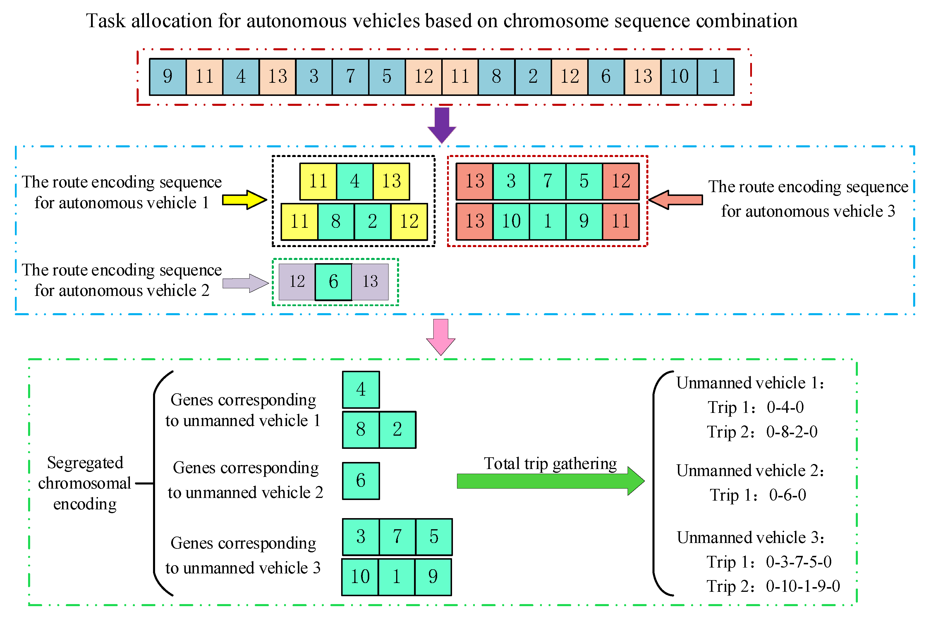
In the MT-CVRP, the coding rules are as follows: assuming that the total number of customer points to be served is n , the total number of transportation vehicles is z , and that each vehicle has, at most, w trips for delivery, this paper plans to use these integers for chromosome coding, while the coding length of the whole chromosome is n + w × z . First of all, we generate the w × z matrix K , the customer’s 1 n integer and matrix K are integrated into a row vector, and then we randomly generate the length of the n + w × z chromosome sequence, representing a chromosome. At the same time, expressed as a solution to the problem, the entire chromosome encoding sequence corresponds to the actual problem; assuming that all vehicles z in the K matrix virtualize one distribution center for each distribution trip they make, all trips should virtualize w distribution centers. The corresponding decoding rules are as follows: firstly, based on the coding rules, the n + w × z alleles are randomly arranged to locate the position of gene sequences within the integer n n + w × z range; secondly, the current coding of n n + w × z alleles is used to divide the trips into a number of gene segments, which in turn determine the sequences of all the customers distributed to by each vehicle.
Figure 2 shows the coding and decoding schematic of the IGA to solve the MT-CVRP. Assuming that there are 3 vehicles to serve 10 customers and that each vehicle has at most 2 trips, K = 11 , 12 , 13 ; 11 , 12 , 13 ; this is followed by integrating the integers from 1 to 10 with the matrix K to form a vector, and finally generating the chromosome sequence randomly. In Figure 2, 1 10 indicates the customer code, the division symbol 11 13 is used to divide the trip, the customer sequence between 2 adjacent separator symbols constitutes a trip, the same divider is used to specify the unmanned vehicle transportation task of the trip task set, the unmanned vehicle number and the K value are not needed to distinguish between the randomly specified sequences, and, in terms of the customers to serve, the order of the actual decoding permutation shall prevail.

3.2. Calculation of Adaptation

While the above encoding method cannot ensure that every decoded delivery route satisfies the vehicles’ loading capacity and maximum delivery time constraints, this paper employs the method’s objective function as its fitness function.
F i t n e s s = F

3.3. Selection

In this paper, a binary tournament strategy will be used for the selection operation [49]. This involves randomly selecting two individuals, comparing their fitness, and choosing the individual with the better fitness as the winner. The winner becomes the parent individual for reproduction and is copied into the next generation of the population. This process is repeated until a sufficient number of parent individuals are selected for the reproduction operation.

3.4. Crossing

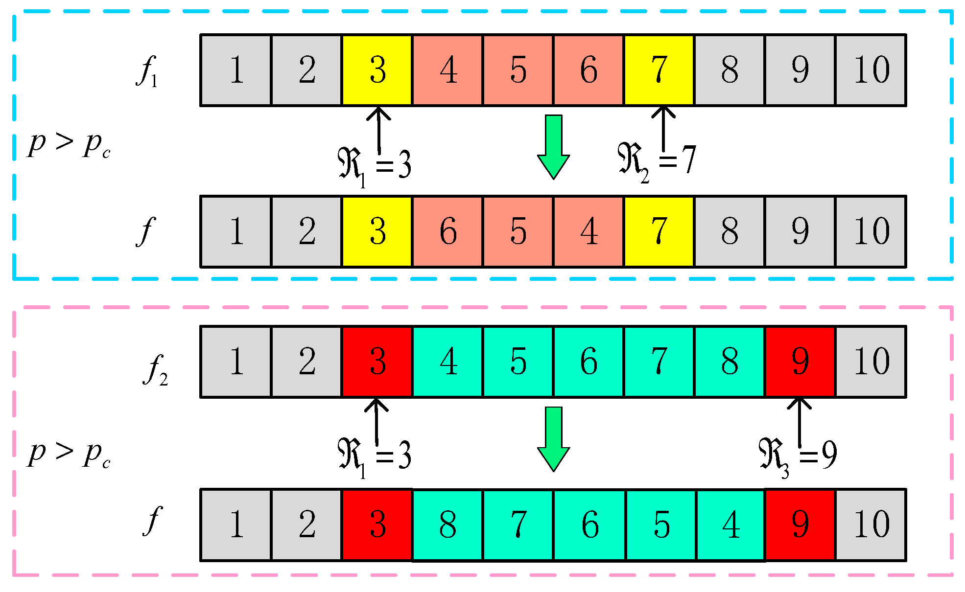
After completing population selection, individuals in the population need to undergo a crossover operation. The crossover operation used in this paper differs from traditional genetic algorithms in that it is based on a combination of generating random numbers and crossover probabilities. It selectively completes chromosome crossover and then performs gene inversion. The idea behind this crossover operation is to make the best use of the information obtained from the population to guide individuals towards the optimal direction of evolution, making the genetic operator more efficient, as shown in Figure 3. The specific steps are as follows:
  • Randomly select a gene spot 1 in the paternal chromosome f 1 , e.g., 1 = 3 ;
  • Generate a random decimal number p within the range of [0, 1]; if p < p c , then select a second gene point 2 in the parent chromosome f 1 , such as 2 = 7 . Invert the partial chromosome sequence between gene point 1 and gene point 2 to produce a new chromosome f , which does not include the 1 and 2 gene points, which is similar to the principle of 2-Opt algorithm operation;
  • If p > p c is selected, then another paternal chromosome f 2 is selected from the population to determine the location of 1 = 3 , and the next gene point 3 = 9 . If the gene point 3 is selected from chromosome f 2 , the previous gene point will be taken if it is out of bounds; similarly, the portion of the chromosome between the gene point 1 = 3 and the gene point 3 = 9 will be inverted to exclude the 1 and 3 gene points.

3.5. Mutation

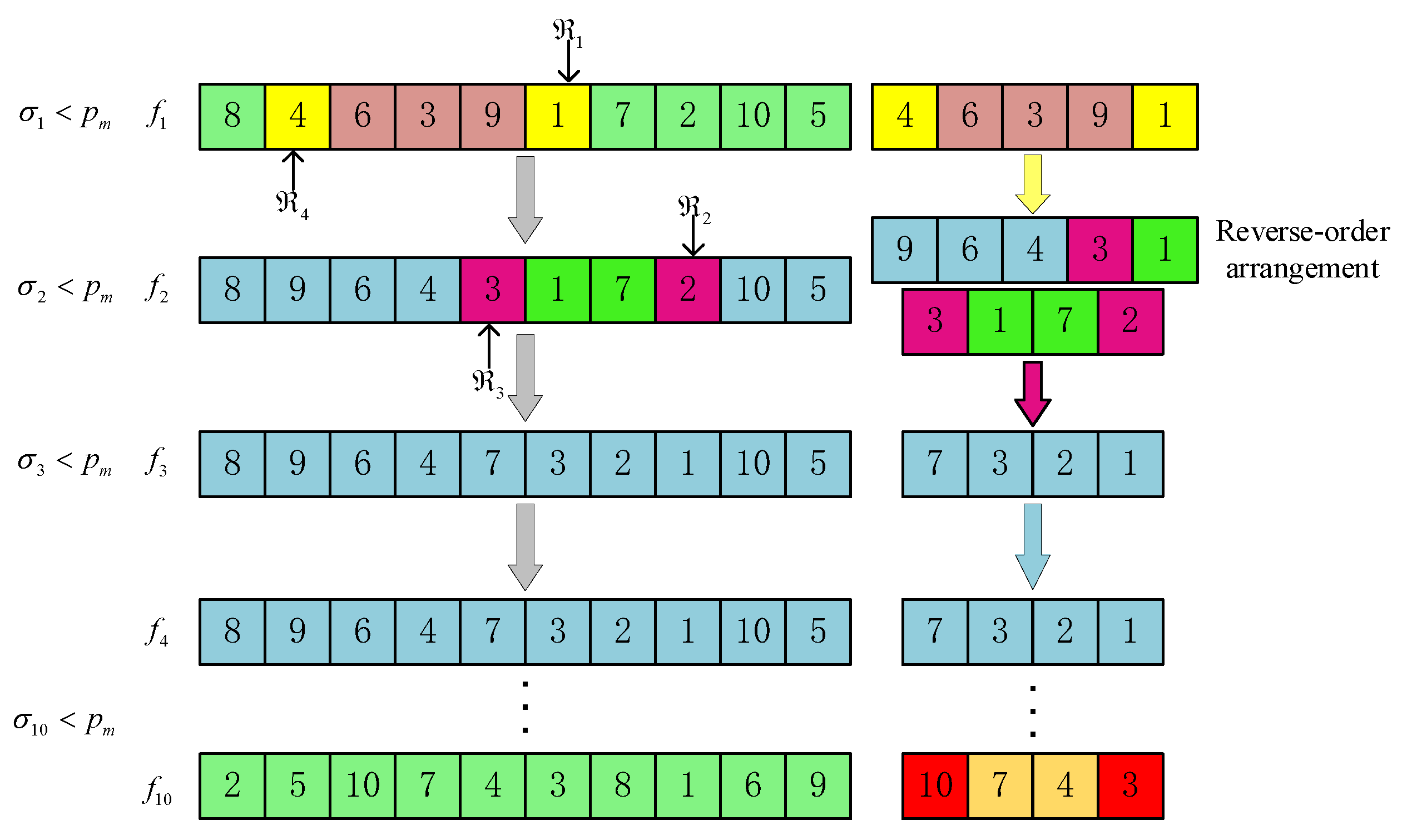
To ensure that the population evolves in a favorable direction and quickly finds satisfactory solutions, a mutation operation is performed on the offspring population after completing the crossover operation. In traditional methods, mutation only occurs when the chromosome is greater than a random number. However, the proposed method in this paper focuses on mutating every gene of every chromosome. Each time, a random number is generated and the mutation of the gene position is determined by both the mutation probability and the random number, thus accelerating the generation of optimal solutions for the population. As shown in Figure 4, the specific operation is as follows:
  • Assuming that the length of chromosome f 1 is N = 10 , firstly, for the 1st gene 1 , generate a random number σ 1 , if σ 1 < p m , generate a random number 1 of 1 N , 1 = 4 , 1 = 4 , mapped to gene 4 , which forms the sequence of genes between alleles 1 4 of the chromosome, in accordance with their subscripts, from smallest to largest, in order, and, after the reverse order of the sequence is embedded in f 1 (including 1 , 4 ), at this time observe the chromosome f 2 ; if σ 1 > p m , then do not generate a random number, and do not do anything with the 1 gene;
  • For the gene 2 , if the random number σ 2 < p m , a random number 1 N is generated 2 . 2 = 3 is mapped to the gene 3 , and the chromosome allele between 2 3 is embedded in f 2 after a reverse-ordering process, at which point the chromosome is f 3 ; if σ 2 > p m , no random number is generated, and no processing is carried out for the 2 gene;
  • Continue to repeat the above steps until all the alleles of the entire chromosome have been traversed to complete the mutation operation.

3.6. Repair Operation

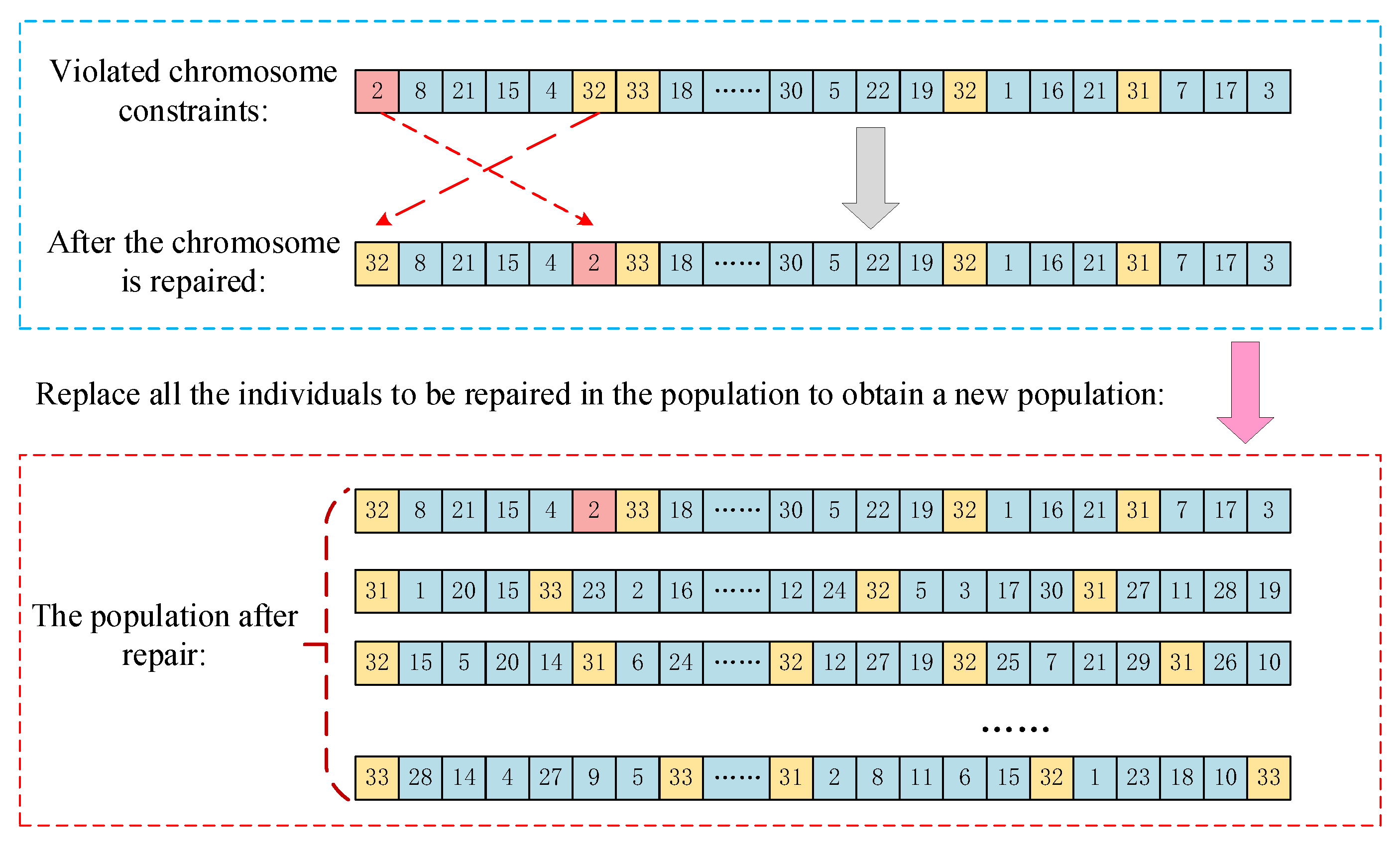
There is a problem in the above encoding and decoding process. Each trip involves the issue of the virtual distribution center. The starting point of each unmanned vehicle must be the virtual distribution center w , so the first gene position of the chromosome individual must be the gene representing w . However, in the evolutionary algorithm, both the individual initialization and the gene sequence disorder caused by the evolution may not satisfy the condition of gene w being in the first position. Therefore, before decoding the population’s individuals, a repair operation is required. The specific approach is that if the first gene of the individual is the customer point n gene instead of the distribution center gene w , then the first distribution center gene found, from left to right, is swapped with the first gene. As shown in Figure 5, if n = 30 , w = z = 3 , thus the first gene of the chromosome violates the constraint by being the customer point gene n , representing the number 2. After checking the chromosome, it is found that the virtual distribution center gene w is 32. Therefore, the two genes are swapped to obtain a repaired individual. After repairing all individuals, a new population is obtained.

3.7. Simulated Annealing Algorithm

GAs have the properties of global optimality and robustness, but they tend to become stuck in local optima. On the other hand, the SAs have the advantage of escaping local optima. Therefore, a simulated annealing operator will be introduced into the mutation operation [16]. The simulated annealing operator is introduced into the new population after crossover, mutation, and repair, and gene points within the range of 1 ~ ( n + w × z ) are randomly selected with the mutation probability p m , and an inferior solution is accepted with a probability p . If the virtual distribution center is selected, the genes in the sequence of n n + w × z are selected to be swapped with the gene sites in the same range, and the mutation operation is performed n + w × z / 2 times for each chromosome, with the following acceptance probabilities [50]:
p = e Δ F / F max Δ F     0 1       Δ F   <   0
where Δ F is the value of the fitness change in the chromosome before and after its mutation and F max is the highest fitness value in the current chromosome.

3.8. Elite Retention Strategies

To prevent genetic algorithms from losing the best individual in their current population during iterations, an elite preservation strategy has been introduced. This strategy aims to improve the algorithm’s global convergence capability by storing the individuals with the highest fitness, thereby retaining excellent individuals [51].

3.9. Algorithmic Flow

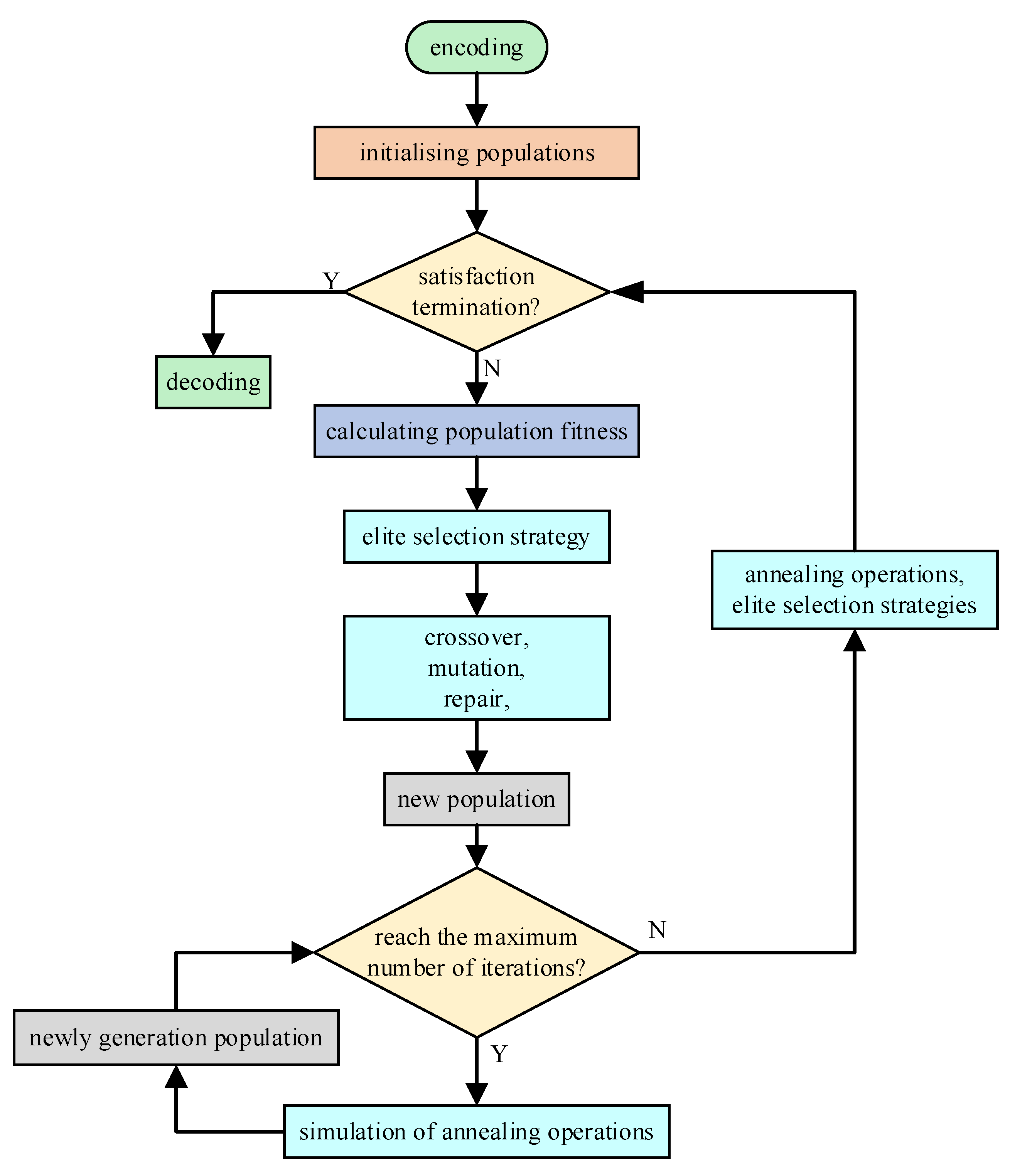
Based on the above analysis, the algorithm’s flow is shown in Figure 6, and the algorithm framework of the IGA is displayed in Algorithm 1.
Algorithm 1 IGA
Input: Algorithm-related parameters and simulation base data
Output: Multi-trip solutions for unmanned vehicles
1. encoding, initializing the IGA algorithm and setting parameters
2. mapping the problem and randomly generating a certain size of the population
3.     if the initialization scheme satisfies the set constraints, then
4.     decoding
5.      else
6.      calculating the fitness value and performing elite selection, crossover, mutation, and repair operations
7.      else
8.        if the maximum number of iterations is reached, then performing cooling and elite selection
9.        else
10.           implementation of simulated annealing operations
11.      end if
12.      break
13.   end if
The principle of the annealing operator is that new individuals are the first generated, and if the new individuals are better than the old ones, they are accepted and passed on to the next generation of the population. If the new individual is worse than the old one, the new individual is accepted with a specific probability.

4. Simulation Test and Result Analysis

4.1. Calculations and Parameterizations

The simulation data for the experiment and testing of the model and algorithm were conducted using the Solomon RC 208 dataset [52], and the simulation results were compared across small-scale, medium-scale, and large-scale operations of the GA. According to reference [13], the relevant parameters are set as follows: the population size of G max is 100, the crossover probability p c is 0.9, the variance probability p m is 0.01, the cooling coefficient θ is 0.95, the initial temperature T 0 is 100 °C, and the termination temperature T e is 1 °C. The parameters for the SA are as follows: the initial temperature is 200, the final temperature is 1, the cooling rate is 0.8, and the chain length is 200 [37]. The parameters for the GA are as follows: the population size is 100, the crossover probability is 0.8, and the mutation probability is 0.2 [47]. The cost γ of traveling 1 km in an unmanned vehicle is USD 1, there is a startup cost θ 1 of USD 200 per unmanned vehicle, the cost per liter of fuel θ 2 is USD 6.8, the environmental cost per 1 kg of CO2 emitted θ 3 is USD 1.2, the fuel consumption per kilometer ε is 0.3 L, the fuel conversion coefficient ρ is 2.36 kg CO2 /L, the penalty cost per unit of the unmanned vehicle’s total trip delivery time exceeding its maximum driving time λ is USD 30/kg, and the penalty cost per unit exceeding the vehicle’s rated load η is USD 20/kg.

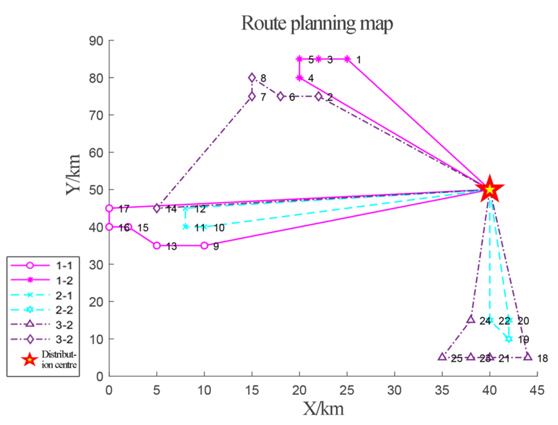
4.2. Simulation of Small-Scale Cases

Assuming that the distribution center utilizes unmanned vehicles to deliver goods to 25 supermarkets, we use the Solomon RC 208 dataset (25) [52] for the first 25 sample data points. It is assumed that a maximum of five vehicles are available, each able to make a maximum of two trips. The vehicles’ capacity is 90 kg, with a speed of 50 km/h, and the maximum delivery duration is 5 h. The maximum number of generations, for both algorithms, is set to 300. We ran the program five times for each of the three algorithms and selected the best result. Figure 7 shows the optimization results of the IGA, and Figure 8 displays the evolution curve of the three algorithms, including the change trend of their maximum fitness curves and average fitness curves. The data results for both algorithms are shown in Table 3, where the total cost deviation rate = (GA−IGA)/IGA, reflecting the algorithms’ degree of deviation from the optimal solution. On the delivery route maps, the legend “1-1” represents the first delivery by unmanned vehicle 1, and “1-2” represents the second delivery by unmanned vehicle 1. The optimized delivery scheme for unmanned vehicles using the IGA is shown in Table 4.

4.3. Simulating Medium-Scale Cases

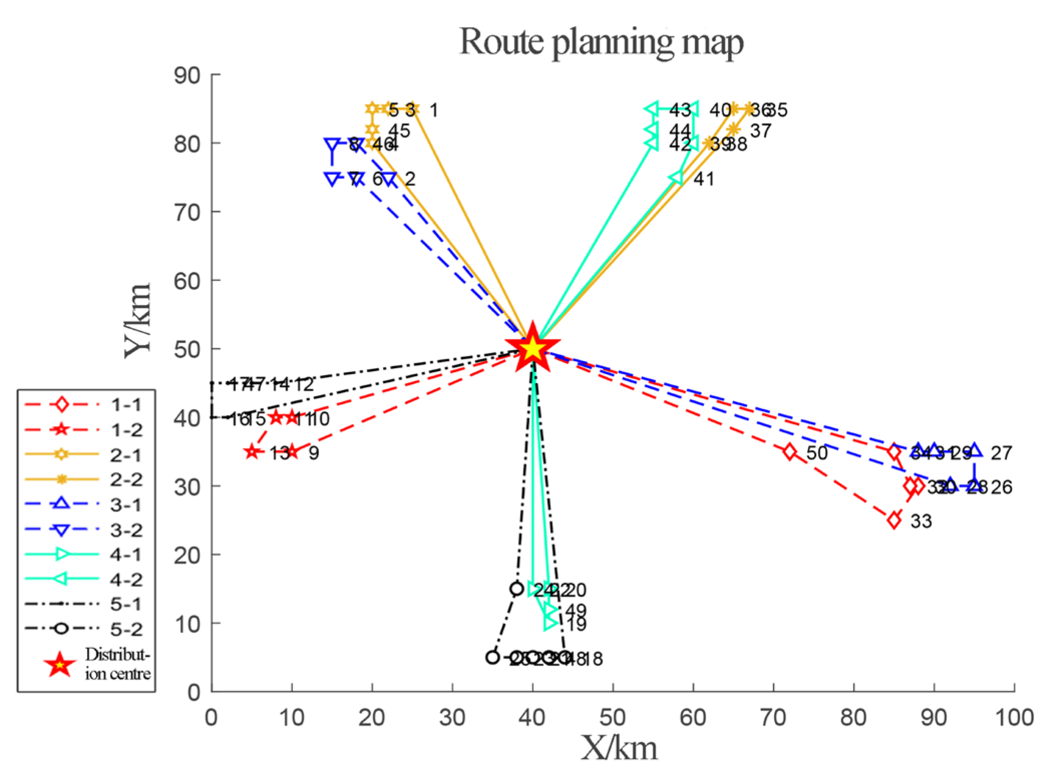
Assuming that the distribution center employs unmanned vehicles for deliveries to 50 supermarkets, the Solomon RC 208 dataset (50) [52] is utilized, using its first 50 sample data points. The parameter settings differ from the small-scale examples in that unmanned vehicles can make a maximum of three trips and the vehicles’ capacity is 100 kg. The unmanned vehicle’s speed and maximum delivery time remain constant. Three algorithms underwent 1600 evolutions. Following five program runs, Figure 9 illustrates the delivery routes generated using the IGA. Figure 10 presents the population evolution graph for the three algorithms. The simulation results are detailed in Table 5, and the optimized delivery scheme for unmanned vehicles using the IGA is shown in Table 6.

4.4. Simulation of Large-Scale Cases

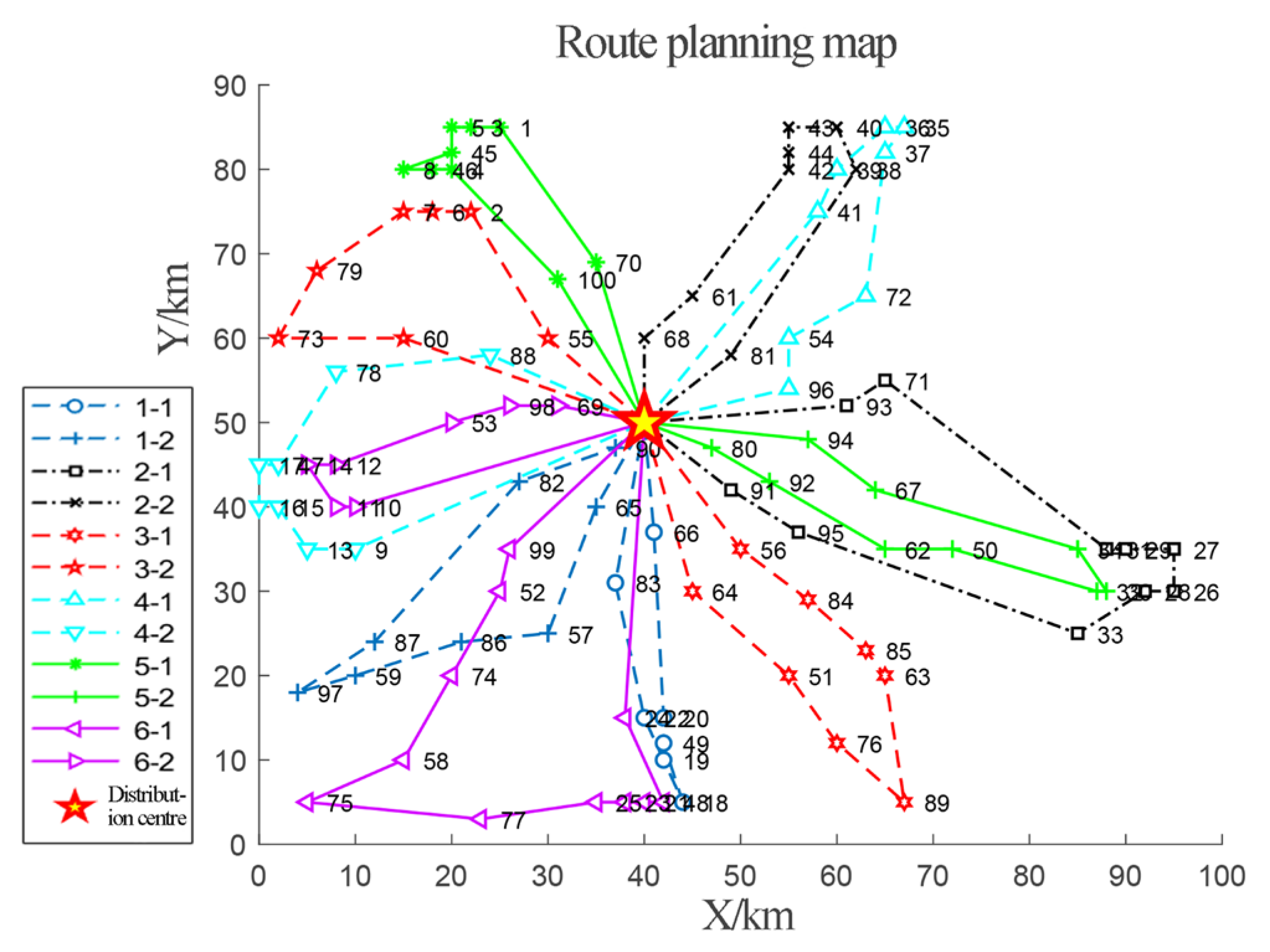
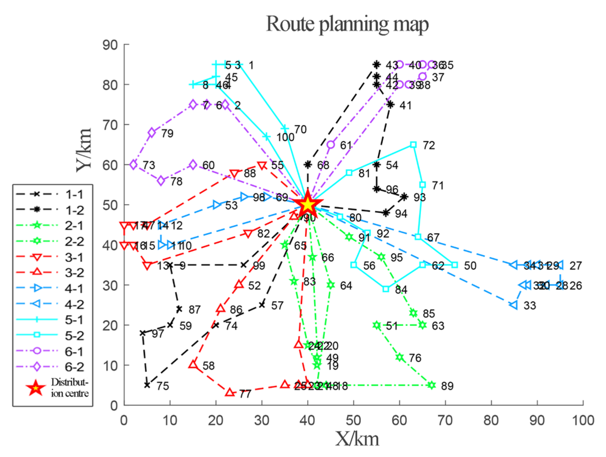
Assuming that a distribution center employs unmanned vehicles for delivering to 100 supermarkets, using the Solomon RC 208’s [52] sample data, the large dataset prompts adjustments to the parameter settings compared to medium-scale cases. Specifically, six unmanned vehicles are available, each with a maximum of three trips. The vehicle capacity is set to 150 kg, while the unmanned vehicles’ speed and maximum delivery time remain constant. The maximum number of evolutions for all algorithms is established at 12,000. The program undergoes five runs, and Figure 11 illustrates the unmanned vehicle delivery route maps generated using the IGA. Figure 12 displays the population evolution curves of the three algorithms. The algorithm run results are detailed in Table 7, and the optimized delivery scheme for unmanned vehicles, using the IGA, is shown in Table 8.
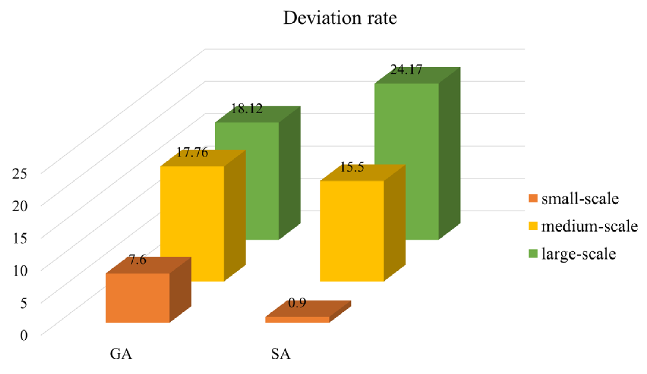
Based on simulation data of different scales, the deviation rate was plotted as is shown in Figure 13.
Our conclusions are as follows:
  • Based on graphs 8, 10, and 12, it can be observed that the IGA achieves convergence at a faster rate than the GA and SA. In these graphs, the fitness value remains unchanged at the 212th, 580th, and 3850th iterations of the IGA, respectively. Additionally, as the problem size increases, the difference in fitness values becomes more pronounced, indicating that the IGA not only provides better solutions but also exhibits good convergence speed.
  • Analyzing the total cost deviation rate in Figure 13, it can be seen that, compared to the GA, the IGA yields lower deviation rates of 7.6%, 17.76%, and 18.12% for small, medium, and large problem sizes, respectively. Similarly, compared to the SA, the deviation rates for the IGA are 0.97%, 15.5%, and 24.17% for those respective problem sizes. These results demonstrate that the IGA consistently outperforms the other two algorithms. In smaller and medium-sized problems, the SA performs better than the GA, while in larger problems the GA outperforms the SA.
  • With the same problem size, the number of autonomous vehicles may vary, leading to different startup costs. In the simulations of small to large problems, the startup costs of the vehicles account for 22.23%, 21.43%, and 19.95% of the total cost, respectively. This ratio gradually decreases with an increase in the number of customers. Additionally, due to the varying number of autonomous vehicles and their routes during the delivery process, the fuel cost, environmental cost (CO2 emissions), and total delivery duration also vary significantly.
  • Table 4, Table 6 and Table 8 provide the optimal delivery plans obtained, using the IGA, for different problem sizes. These tables include the plans, lengths, and load capacities of each route, as well as the total route length and overall delivery duration. As the problem size increases, the number of dominated autonomous vehicles also increases. However, whether for small, medium, or large problem sizes, all autonomous vehicle delivery trips adhere to the constraints of the vehicles’ load capacity and maximum delivery duration. This indicates that the algorithm effectively considers the constraints of the model during the optimization process, without adding penalty costs to the total cost.

5. Sensitivity Analysis

5.1. Compared with Single-Route Delivery by Unmanned Vehicles

Using the E-n51-k5 international standard dataset as a reference, the IGA, with unchanged parameters, was independently run 10 times to obtain its average values. The results of this comparison for different routes are shown in Table 9, with the deviation rate calculated as (multi-route−single-route)/multi-route × 100%.
Firstly, from the simulated data results it can be observed that, relative to the multi-route delivery of unmanned vehicles, single-route delivery can reduce the total delivery time of the solution, but it requires more unmanned vehicles to complete the task, leading to an increase in startup costs and, consequently, an increase in total costs.
Secondly, in terms of the number of unmanned vehicle startups, the algorithm in this study requires three fewer vehicles compared to single-route delivery, and one fewer vehicle compared to the approach in reference [44]. Additionally, its total distance is significantly reduced by 41.27 km compared to the approach in reference [44]. Multi-route delivery can greatly reduce the number of unmanned vehicles needed, which brings the benefit of saving vehicle startup costs but also entails corresponding transportation costs.
Lastly, when considering which measure to adopt for distributions in practical logistics, a comprehensive assessment should be made considering various factors.

5.2. Deliveries Using Different Vehicle Models

We used the medium-scale Solomon RC 208 (50) sample data as a reference and employed three different vehicle models with unmanned vehicle carrying capacities of 100 kg, 150 kg, and 200 kg; startup costs of USD 200, USD 300, and USDE 500; and transportation costs per unit distance of USD 1, USD 3, and USD 6, respectively. There were five unmanned vehicles at the distribution center, and their maximum delivery time was 8 h. The simulation results, obtained by running the simulation independently 10 times and averaging the values, are shown in Table 9, with the deviation rate calculated as (worst value−best value)/best value × 100%. Several deep-level analysis results can be derived from the data in Table 10.
Firstly, our analysis reveals that the fuel cost of the 100 kg low-capacity unmanned vehicle constitutes the highest proportion of the total cost, approximately 41%. This indicates that low-capacity vehicles tend to consume more fuel, potentially necessitating more frequent charging or refueling, consequently elevating their share of fuel costs. To mitigate fuel costs, logistics companies may contemplate the adoption of unmanned vehicles with higher payload capacities.
Secondly, compared to low-load unmanned vehicles, those with higher load capacities exhibit a notable reduction in their total trips, average trips, total delivery duration, and total distance. This suggests that vehicles with higher load capacities can reduce their trips and distances during delivery, leading to reduced total delivery duration and costs. Logistics companies can prioritize using high-load-capacity vehicles to enhance their efficiency and cost-effectiveness.
Moreover, an increase in payload capacity correlates with a gradual rise in the proportion of transportation costs within the total delivery costs. This implies that transportation costs exert a growing influence on overall costs. As their payload capacity increases, logistics companies must allocate more resources to supporting transportation tasks, resulting in larger transportation costs. Therefore, when selecting unmanned vehicles, logistics companies need to strike a balance between transportation costs and total costs, opting for an appropriate payload capacity to minimize their overall costs.
Lastly, the complete simulation of different vehicle types using the optimization process lasts approximately 20 s, indicating that the algorithm in this study converges rapidly and exhibits strong optimization efficiency. This underscores the algorithm’s commendable optimization performance, demonstrating its ability to identify optimal solutions rapidly.
In summary, in practical operations, logistics companies should comprehensively consider their total costs and carefully choose suitable vehicle types for their operations. While high-load-capacity unmanned vehicles can reduce total delivery durations and costs, it is essential to also account for the proportion of transportation costs within the company’s total costs.

5.3. Consideration of the Impact of Carbon Emissions

Using the large-scale data and parameters of the example in Section 4.4, a simulation of route optimization for customers was conducted without considering the impact of carbon emissions. The simulation ran independently five times to obtain average values, and the results are presented in Table 11. The route planning results are depicted in Figure 16. In the scenario where unmanned vehicles do not use fuel, there are no carbon dioxide emissions or fuel costs. A comparison of the data showed that when carbon emissions are not considered, the total cost is lower than when considering carbon emissions, with a deviation rate of 22.6%. Furthermore, a comparison of the delivery route maps in Figure 11 and Figure 14 reveals that the delivery route map considering carbon emissions has a more clearly organized overall task arrangement, with fewer intersections of the routes of unmanned vehicles, resulting in a more optimized delivery route. In real traffic scenarios, especially during significant traffic congestion, utilizing a low-carbon-emission delivery scheme can effectively optimize carbon emissions. This is because vehicle fuel consumption and carbon emissions are directly proportional and, consequently, reducing carbon emissions also reduces delivery costs. Therefore, selecting a low-carbon-emission delivery scheme not only aligns with businesses’ decision-making needs but also contributes to achieving two carbon goals.

6. Conclusions

To tackle the multi-trip delivery challenge using unmanned vehicles, we reformulate it as the MT-CVRP, with the objective of minimizing total costs. An optimization model is developed, including a consideration of carbon emissions, and an IGA is tailored to address the problem. Simulation validations are conducted, yielding the following results:
  • Using the Solomon RC 208 international standard dataset, simulations were conducted for small-, medium-, and large-scale scenarios, comparing the IGA with the GA and SA. Firstly, the IGA is capable of providing high-quality results in a shorter period of time. Secondly, varying the startup numbers of the autonomous vehicles for different scale distributions leads to differences in their total delivery costs, as well as their fuel expenses, environmental costs (CO2 emissions), and overall delivery durations. Lastly, from the perspective of algorithm effectiveness, by observing the optimal delivery plans generated by the IGA, it is evident that the algorithm satisfies its predetermined constraints across all three scales of scenarios, while possessing strong global search capabilities and high computational efficiency.
  • By employing the E-n51-k5 standard dataset and comparing it with the existing literature [44], multi-trip delivery proves advantageous over single-trip delivery, especially with respect to vehicle startup costs. The choice of delivery strategy hinges on the costs and transportation expenses linked to unmanned vehicles. Unmanned vehicles with a high load capacity can curtail their total number of trips and overall delivery duration. In delivery plans that account for carbon emissions, the routes of unmanned vehicles are optimized.
Optimizing the multi-trip delivery routes of unmanned vehicles has the potential to reduce their mileage and carbon emissions, consequently enhancing air quality, mitigating environmental impacts, improving delivery efficiency, and cutting logistics costs. This research is of substantial value to future applications in sectors such as express delivery, healthcare, manufacturing facilities, and public transportation, ultimately advancing sustainable development. It is crucial to recognize that real-world delivery activities are subject to dynamic factors like vehicle failures and traffic congestion, considerations that should be factored into future studies.

Author Contributions

Conceptualization, X.G. and S.L.; methodology, X.G.; software, X.G.; validation, X.G. and Y.W.; formal analysis, S.L.; investigation, Y.P.; resources, X.G.; data curation, X.G.; writing—original draft preparation, X.G.; writing—review and editing, Y.P. and D.Z.Y.; visualization, Y.P.; supervision, D.Z.Y.; project administration, X.M. and Y.W.; funding acquisition, S.L. and X.G. All authors have read and agreed to the published version of the manuscript.

Funding

This research was funded by Chongqing Doctoral through the Train Project (Grant No. CSTB2022BSXM-JCX0099), the Research and Innovation Program for Graduate Students in Chongqing (Grant No. 2022S0031), and the Team Building Project for Graduate Tutors in Chongqing (Grant No. JDDSTD2022004).

Institutional Review Board Statement

Not applicable.

Informed Consent Statement

Not applicable.

Data Availability Statement

The data presented in this study are available on request from the corresponding author.

Conflicts of Interest

Yan Wang was employed by the company T.Y.LIN International Group Chongqing. The remaining authors declare that the research was conducted in the absence of any commercial or financial relationships that could be construed as a potential conflict of interest.

References

  1. Liu, Z.; Niu, Y.; Guo, C.; Jia, S. A Vehicle Routing Optimization Model for Community Group Buying Considering Carbon Emissions and Total Distribution Costs. Energies 2023, 16, 931. [Google Scholar] [CrossRef]
  2. Severino, A.; Curto, S.; Barberi, S.; Arena, F.; Pau, G. Unmanned vehicles: An Analysis Both on Their Distinctiveness and the Potential Impact on Urban Transport Systems. Appl. Sci. 2021, 11, 3604. [Google Scholar] [CrossRef]
  3. Zhang, S.; Markos, C.; James, J.Q. Autonomous vehicle intelligent system: Joint ride-sharing and parcel delivery strategy. IEEE Trans. Intell. Transp. Syst. 2022, 23, 18466–18477. [Google Scholar] [CrossRef]
  4. Vlachos, I.P.; Pascazzi, R.M.; Zobolas, G.; Repoussis, P.; Giannakis, M. Lean manufacturing systems in the area of Industry 4.0: A lean automation plan of AGVs/IoT integration. Prod. Plan. Control 2023, 34, 345–358. [Google Scholar] [CrossRef]
  5. Wang, N.; Lyu, Y.; Jia, S.; Zheng, C.; Meng, Z.; Chen, J. A dynamic graph-based many-to-one ride-matching approach for shared autonomous electric vehicles. Transportation 2023, 4, 1–27. [Google Scholar] [CrossRef]
  6. Hakak, S.; Gadekallu, T.R.; Maddikunta, P.K.R.; Ramu, S.P.; Parimala, M.; De Alwis, C.; Liyanage, M. Unmanned vehicles in 5G and beyond: A Survey. Veh. Commun. 2022, 39, 100551. [Google Scholar] [CrossRef]
  7. Parekh, D.; Poddar, N.; Rajpurkar, A.; Chahal, M.; Kumar, N.; Joshi, G.P.; Cho, W. A Review on Unmanned vehicles: Progress, Methods and Challenges. Electronics 2022, 11, 2162. [Google Scholar] [CrossRef]
  8. Liu, S.; Gao, X.; Chen, L.; Zhou, S.; Peng, Y.; Yu, D.Z.; Ma, X.; Wang, Y. Multi-Traveler Salesman Problem for Unmanned Vehicles: Optimization through Improved Hopfield Neural Network. Sustainability 2023, 15, 15118. [Google Scholar] [CrossRef]
  9. Zhang, C.; Tang, L.; Zhang, J.; Gou, L. Optimizing Distribution Routes for Chain Supermarket Considering Carbon Emission Cost. Mathematics 2023, 11, 2734. [Google Scholar] [CrossRef]
  10. Chen, X.; Li, Q.; Li, R.; Cai, X.; Wei, J.; Zhao, H. UAV Network Path Planning and Optimization Using a Vehicle Routing Model. Remote Sens. 2023, 15, 2227. [Google Scholar] [CrossRef]
  11. Ito, S.; Akaiwa, K.; Funabashi, Y.; Nishikawa, H.; Kong, X.; Taniguchi, I.; Tomiyama, H. Load and Wind Aware Routing of Delivery Drones. Drones 2022, 6, 50. [Google Scholar] [CrossRef]
  12. Saksuriya, P.; Likasiri, C. Hybrid Heuristic for Vehicle Routing Problem with Time Windows and Compatibility Constraints in Home Healthcare System. Appl. Sci. 2022, 12, 6486. [Google Scholar] [CrossRef]
  13. Guan, Y.; Wang, Y.; Yan, X.; Guo, H.; Zhao, Y. The One E-Ticket Customized Bus Service Mode for Passengers with Multiple Trips and the Routing Problem. Sustainability 2022, 14, 2124. [Google Scholar] [CrossRef]
  14. Cataldo-Díaz, C.; Linfati, R.; Escobar, J.W. Mathematical Model for the Electric Vehicle Routing Problem Considering the State of Charge of the Batteries. Sustainability 2022, 14, 1645. [Google Scholar] [CrossRef]
  15. Baek, D.; Chen, Y.; Chang, N.; Macii, E.; Poncino, M. Battery-Aware Electric Truck Delivery Route Exploration. Energies 2020, 13, 2096. [Google Scholar] [CrossRef]
  16. Zhao, M.; Lu, Y. A Heuristic Approach for a Real-World Electric Vehicle Routing Problem. Algorithms 2019, 12, 45. [Google Scholar] [CrossRef]
  17. Chen, S.; Chen, R.; Gao, J. A Monarch Butterfly Optimization for the Dynamic Vehicle Routing Problem. Algorithms 2017, 10, 107. [Google Scholar] [CrossRef]
  18. Song, R.; Qin, W.; Shi, W.; Xue, X. Optimizing Freight Vehicle Routing in Dynamic Time-Varying Networks with Carbon Dioxide Emission Trajectory Analysis. Sustainability 2023, 15, 15504. [Google Scholar] [CrossRef]
  19. Hachiya, D.; Mas, E.; Koshimura, S. A Reinforcement Learning Model of Multiple UAVs for Transporting Emergency Relief Supplies. Appl. Sci. 2022, 12, 10427. [Google Scholar] [CrossRef]
  20. Cattaruzza, D.; Absi, N.; Feillet, D.; Vigo, D. An iterated local search for the multi-commodity multi-trip vehicle routing problem with time windows. Comput. Oper. Res. 2014, 51, 257–267. [Google Scholar] [CrossRef]
  21. Tan, K.; Liu, W.; Xu, F.; Li, C. Optimization Model and Algorithm of Logistics Vehicle Routing Problem under Major Emergency. Mathematics 2023, 11, 1274. [Google Scholar] [CrossRef]
  22. Hou, B.; Zhang, K.; Gong, Z.; Li, Q.; Zhou, J.; Zhang, J.; de La Fortelle, A. SoC-VRP: A Deep-Reinforcement-Learning-Based Vehicle Route Planning Mechanism for Service-Oriented Cooperative ITS. Electronics 2023, 12, 4191. [Google Scholar] [CrossRef]
  23. Zheng, X.; Gao, F.; Tong, X. Research on Green Vehicle Path Planning of AGVs with Simultaneous Pickup and Delivery in Intelligent Workshop. Symmetry 2023, 15, 1505. [Google Scholar] [CrossRef]
  24. Yang, J.; Zhu, H.; Ma, J.; Yue, B.; Guan, Y.; Shi, J.; Shangguan, L. Improved Genetic Algorithm for Solving Green Path Models of Concrete Trucks. Appl. Sci. 2023, 13, 9256. [Google Scholar] [CrossRef]
  25. Fleischmann, B. The Vehicle Routing Problem with Multiple Use of Vehicles. Ph.D. Thesis, Fachbereich Wirtschaftswissenschaften, Universität Hamburg, Hamburg, Germany, 1990. [Google Scholar]
  26. Hernandez, F.; Feillet, D.; Giroudeau, R.; Naud, O. An exact method to solve the multitrip vehicle routing problem with time windows and limited duration. TRISTAN 2010, 7, 366–369. [Google Scholar] [CrossRef]
  27. Azi, N.; Gendreau, M.; Potvin, J.Y. An exact algorithm for a vehicle routing problem with time windows and multiple use of vehicles. Eur. J. Oper. Res. 2010, 202, 756–763. [Google Scholar] [CrossRef]
  28. Munari, P.; Morabito, R. A branch-price-and-cut algorithm for the vehicle routing problem with time windows and multiple deliverymen. Top 2018, 26, 437–464. [Google Scholar] [CrossRef]
  29. Marques, G.; Sadykov, R.; Dupas, R.; Deschamps, J.C. A branch-cut-and-price approach for the single-trip and multi-trip two-echelon vehicle routing problem with time windows. Transp. Sci. 2022, 56, 1598–1617. [Google Scholar] [CrossRef]
  30. Huang, N.; Li, J.; Zhu, W.; Qin, H. The multi-trip vehicle routing problem with time windows and unloading queue at depot. Transp. Res. Part E Logist. Transp. Rev. 2021, 152, 102370. [Google Scholar] [CrossRef]
  31. Bettinelli, A.; Cacchiani, V.; Crainic, T.G.; Vigo, D. A branch-and-cut-and-price algorithm for the multi-trip separate pickup and delivery problem with time windows at customers and facilities. Eur. J. Oper. Res. 2019, 279, 824–839. [Google Scholar] [CrossRef]
  32. Karimi, L.; Nawrin Ferdous, C. Branch and Price Algorithm for Multi-Trip Vehicle Routing with a Variable Number of Wagons and Time Windows. Algorithms 2022, 15, 412. [Google Scholar] [CrossRef]
  33. Karoonsoontawong, A.; Kobkiattawin, O.; Xie, C. Efficient insertion heuristic algorithms for multi-trip inventory routing problem with time windows, shift time limits and variable delivery time. Netw. Spat. Econ. 2019, 19, 331–379. [Google Scholar] [CrossRef]
  34. Petch, R.J.; Salhi, S. A multi-phase constructive heuristic for the vehicle routing problem with multiple trips. Discret. Appl. Math. 2003, 133, 69–92. [Google Scholar] [CrossRef]
  35. Brandao, J.; Mercer, A. A tabu search algorithm for the multi-trip vehicle routing and scheduling problem. Eur. J. Oper. Res. 1997, 100, 180–191. [Google Scholar] [CrossRef]
  36. Olivera, A.; Viera, O. Adaptive memory programming for the vehicle routing problem with multiple trips. Comput. Oper. Res. 2007, 34, 28–47. [Google Scholar] [CrossRef]
  37. Babaee Tirkolaee, E.; Abbasian, P.; Soltani, M.; Ghaffarian, S.A. Developing an applied algorithm for multi-trip vehicle routing problem with time windows in urban waste collection: A case study. Waste Manag. Res. 2019, 37, 4–13. [Google Scholar] [CrossRef]
  38. Tirkolaee, E.B.; Hosseinabadi, A.A.R.; Soltani, M.; Sangaiah, A.K.; Wang, J. A Hybrid Genetic Algorithm for Multi-Trip Green Capacitated Arc Routing Problem in the Scope of Urban Services. Sustainability 2018, 10, 1366. [Google Scholar] [CrossRef]
  39. Tirkolaee, E.B.; Goli, A.; Bakhsi, M.; Mahdavi, I. A robust multi-trip vehicle routing problem of perishable products with intermediate depots and time windows. Numer. Algebra Control. Optim. 2017, 7, 417–433. [Google Scholar] [CrossRef]
  40. Zhang, X.N.; Fan, H. Multi-trip fuzzy demand vehicle path optimization with time window preferences. Comput. Integr. Manuf. Syst. 2018, 24, 2461–2477. Available online: https://kns.cnki.net/kcms/detail/11.5946.TP.20180108.1722.004.html (accessed on 25 April 2017).
  41. Zhen, L.; Ma, C.; Wang, K.; Xiao, L.; Zhang, W. Multi-depot multi-trip vehicle routing problem with time windows and release dates. Transp. Res. Part E Logist. Transp. Rev. 2020, 135, 101866. [Google Scholar] [CrossRef]
  42. Chen, D.; Pan, S.; Chen, Q.; Liu, J. Vehicle routing problem of contactless joint distribution service during COVID-19 pandemic. Transp. Res. Interdiscip. Perspect. 2020, 8, 100233. [Google Scholar] [CrossRef]
  43. Song, Q. Application of an optimized beam-PSO algorithm in multi-trip vehicle routing problem. Comput. Eng. Sci. 2019, 41, 1882–1891. Available online: https://kns.cnki.net/dm/manage/export.html?filename=CJFDLAST2019!JSJK201910024!1!0&displaymode=NEW&uniplatform=NZKPT (accessed on 13 August 2018).
  44. Song, Q.; Liu, L.X. Research on Multi-Trip Vehicle Routing Problem and Distribution Center Location Problem. Math. Pract. Underst. 2016, 46, 103–113. Available online: https://www.cqvip.com/qk/93074x/201607/668483120.html (accessed on 7 November 2015).
  45. Wassan, N.; Wassan, N.; Nagy, G.; Salhi, S. The multiple trip vehicle routing problem with backhauls: Formulation and a two-level variable neighbourhood search. Comput. Oper. Res. 2017, 78, 454–467. [Google Scholar] [CrossRef]
  46. Neira, D.A.; Aguayo, M.M.; De la Fuente, R.; Klapp, M.A. New compact integer programming formulations for the multi-trip vehicle routing problem with time windows. Comput. Ind. Eng. 2020, 144, 106399. [Google Scholar] [CrossRef]
  47. Anggodo, Y.; Ariyani, A.; Ardi, M.; Mahmudy, W. Optimization of multi-trip vehicle routing problem with time windows using genetic algorithm. J. Environ. Eng. Sustain. Technol. 2017, 3, 92–97. [Google Scholar] [CrossRef]
  48. Janinhoff, L.; Klein, R.; Scholz, D. Multitrip vehicle routing with delivery options: A data-driven application to the parcel industry. OR Spectrum 2023, 1–54. [Google Scholar] [CrossRef]
  49. Sahoo, B.M.; Pandey, H.M.; Amgoth, T. A genetic algorithm inspired optimized cluster head selection method in wireless sensor networks. Swarm. Evol. Comp. 2022, 75, 101151. [Google Scholar] [CrossRef]
  50. Han, J.; Liu, Y.; Li, Y. Vehicle Routing Problem with Drones Considering Time Windows and Dynamic Demand. Appl. Sci. 2023, 13, 13086. [Google Scholar] [CrossRef]
  51. Wang, F.; Ge, X.; Li, Y.; Zheng, J.; Zheng, W. Optimising the Distribution of Multi-Cycle Emergency Supplies after a Disaster. Sustainability 2023, 15, 902. [Google Scholar] [CrossRef]
  52. Solomon, M.M. Algorithms for the vehicle routing and scheduling problems with time window constraints. Oper. Res. 1987, 35, 254–265. [Google Scholar] [CrossRef]
Figure 1. Schematic diagram of MT-CVRP problem.
Sustainability 16 02357 g001
Figure 2. Schematic diagram of MT-CVRP’s coding and decoding.
Sustainability 16 02357 g002
Figure 3. Schematic diagram of crossover operation.
Sustainability 16 02357 g003
Figure 4. Schematic diagram of mutation operation.
Sustainability 16 02357 g004
Figure 5. Population restoration diagram.
Sustainability 16 02357 g005
Figure 6. IGA flow chart.
Sustainability 16 02357 g006
Figure 7. Delivery route map using the IGA.
Sustainability 16 02357 g007
Figure 8. Population evolution graph.
Sustainability 16 02357 g008
Figure 9. Delivery route map using the IGA.
Sustainability 16 02357 g009
Figure 10. Population evolution graph.
Sustainability 16 02357 g010
Figure 11. Delivery route map using the IGA.
Sustainability 16 02357 g011
Figure 12. Population evolution graph.
Sustainability 16 02357 g012
Figure 13. Comparison chart of the deviation rates of the total cost.
Sustainability 16 02357 g013
Figure 14. Path planning diagram without considering carbon emissions.
Sustainability 16 02357 g014
Table 1. A representative comparison of the relevant literature.
PapersOptimization ModelsSolution Method
Research TopicsResearch
Object
Objective FunctionPrecision
Algorithms
Heuristics
Algorithms
Others
Zhang et al. [9]A vehicle routing problem with time windows (VRPTW)Family medical servicesMinimize travel costs Particle Swarm Optimization (PSO)
Chen et al. [10]VRPTask assignmentMinimize the maximum observation timeCPLEX and Gurobi solvers
Guan et al. [13]VRPCustomized busMaximizing profits GA
Zhao et al. [16]Electric Vehicle Routing Problem (EVRP)Electric vehicle servicesMinimize operating costs Adaptive large neighborhood search (ALNS)
Hachiya et al. [19]VRPUnmanned aerial vehicle (UAV)Minimizing total costs Q-learning (QL)
Zheng et al. [23]Green Vehicle Routing Problem Involving Simultaneous Pickup and Delivery with Time Windows (GVRPSPDTWs)The green automated guided vehicle (AGV)’s energy consumptionMinimizing total energy costs Hybrid differential evolution algorithm based on large neighborhood search (DE-LNS)
Yang et al. [24]The Green VRPCommercial concrete distributionMinimizing total fuel consumption GA
Hernandez et al. [26]MTVRPVehicle deliveryMinimize time spent visiting customersBranching and pricing algorithms
Marques et al. [29,31]A multi-trip vehicle routing problem with time windows (MTVRPTW)Delivery of goods to customersMinimization of transport costs Branch-Cut-and-Price approach
Brandao et al. [35]A multi-trip vehicle routing and scheduling problem (MTVRSP)Real distribution problemsAccess to all customers and minimal time spent Tabu search heuristic
Babaee et al. [37]MTVRPMunicipal waste recyclingMinimize total cost of ownership SA
Tirkolaee et al. [38]The multi-trip Green Capacitated Arc Routing Problem (G-CARP)Environmentally friendly emissions of greenhouse gasesMinimizing the cost of greenhouse gas emissions Hybrid Genetic Algorithm (HGA)
Tirkolaee et al. [39]MTVRPPerishable productsMinimizing total distance traveled and total costCPLEX solver
Chen et al. [42]Multi-vehicle multi-trip routing problemCommunity courier delivery serviceResidents’ satisfaction with food delivery services Artificial bee colony algorithm (ABC)
Wassan et al. [45]A Multiple Trip Vehicle Routing Problem with Backhauls (MT-VRPB)Arranging shipments from distribution centers CPLEX solver The Two-Level VNS algorithm
Neira et al. [46]A multi-trip vehicle routing problem with time windows, service-dependent loading times, and limited trip durations (MTVRPTW-SDLT)Vehicle deliveriesReduce costs Two integer programming (IP) models
Anggodo et al. [47]A multi-trip vehicle routing problem with time windows (MTVRPTW)Travel route issuesMinimal commuting time GA
Janinhoff et al. [48]A multi-trip vehicle routing problem with delivery options (MT-VRPDO)Express deliveryMinimizing delivery costs Adaptive large neighborhood search (ALNS)Data-driven framework
Table 2. Notations for the MT-CVRP.
Parameter SymbolsSpecific MeaningUnits
Set:
N The set of customers, denoted as N = 1 , 2 , , n -
Z The set of vehicles, denoted as Z = 1 , 2 , , z -
V The set of all points, denoted as V = 0 N -
A The set of all edges, denoted as A = i , j i , j V -
Parameters:
Q The carrying capacity of the unmanned vehiclekg
D i The demand of customer i kg
d i j The distance between customer i and customer j km
t i j The time at which the unmanned vehicle has passed through customer i and customer j h
γ The cost per unit distance traveled by the unmanned vehicleUSD/km
θ 1 The startup cost for each unmanned vehicleUSD
θ 2 Cost per liter of fuelUSD
θ 3 The environmental cost of emitting 1 kg of CO2USD/kg CO2
ε The vehicle’s fuel consumption per kilometerL/km
ρ The fuel conversion coefficientKg CO2/L
λ The penalty cost for the unmanned vehicle’s total delivery time exceeding its maximum driving timeUSD/h
η The penalty cost per unit for exceeding the vehicle’s rated load capacityUSD/kg
γ A large positive number-
M T The maximum delivery time for each trip during unmanned vehicle deliveryH
M V The maximum number of vehicles that can be used for unmanned vehicle deliveryvehicles
Intermediate variables:
τ w z The sequence in which customers are to be serviced by unmanned vehicle z on trip w -
n z All trips of unmanned vehicle z -
β w z The departure time of unmanned vehicle z on trip w H
δ w z The travel time of unmanned vehicle z on trip w H
Ψ ( τ w z ) The load capacity of unmanned vehicle z on trip w Kg
d i j z The distance traveled by unmanned vehicle z Km
ξ z The set of all trips of unmanned vehicle z -
Decision variables
Y z Is 1 if unmanned vehicle z is activated, otherwise 0-
X i j z w Is 1 if unmanned vehicle z serves customer i and j on trip w , otherwise 0-
Table 3. Comparison of algorithm results.
AlgorithmTotal Cost
(USD)
Vehicle Startup
Cost (USD)
Fuel
Cost (USD)
Environmental Cost (USD)Total Distance
(km)
Number of Unmanned
Vehicles
Total Number of TripsTotal Delivery
Time (h)
Deviation Rate (%)
IGA2698.876001100.70458.61539.563610.78-
GA2903.778001103.27459.68540.824610.827.60
SA2725.166001114.49464.35546.323610.930.97
Table 4. Optimized delivery scheme for unmanned vehicles using the IGA.
Unmanned VehicleRoute ProgramsRoute
Capacity (kg)
Route
Length (km)
Total Line Length (km)Route
Distribution Time (h)
Total Distribution Time (h)
10-9-13-15-16-17-0
0-4-5-3-1-0
90
90
91.68
84.13
175.811.83
1.68
3.51
20-10-11-12-0
020-19-22-0
90
90
71.01
80.44
151.451.42
1.61
3.03
30-24-25-23-21-18-0
02-6-8-7-14-0
90
90
99.67
112.61
212.281.99
2.25
4.24
Table 5. Comparison of algorithm results.
AlgorithmTotal Cost
(USD)
Vehicle Startup
Cost (USD)
Fuel
Cost (USD)
Environmental
Cost (USD)
Total
Distance
(km)
Number of Unmanned
Vehicles
Total Number of
Trips
Total Delivery Time (h)Deviation Rate (%)
IGA4665.8310001869.57778.95916.4651018.31-
GA5494.6510002292.27955.071123.6651122.4817.76
SA4738.1710001887.59786.46925.2951118.5115.50
Table 6. Optimized delivery scheme for unmanned vehicles using the IGA.
Unmanned VehicleRoute ProgramsRoute
Loading Capacity (kg)
Route
Length (km)
Total Line Length (km)Route
Distribution Time (h)
Total Distribution Time (h)
10-1-3-5-45-4-010084.1384.131.681.68
20-50-34-31-0
0-9-13-15-16-17-47-0
80
100
101.63
91.7
193.32.03
1.83
3.86
30-33-32-30-28-26-27-29-0
0-38-36-35-37-0
100
100
127.06
89.25
216.312.54
1.78
4.32
40-42-44-43-40-39-41-0
0-2-46-8-7-6-0
0-12-14-11-10-0
100
90
100
84.73
81.51
74.84
241.081.69
1.63
1.50
4.82
50-24-19-49-22-0
0-20-18-48-21-23-25-0
100
100
82.07
99.53
181.61.64
1.99
3.63
Table 7. Comparison of algorithm results.
AlgorithmTotal Cost
(USD)
Vehicle Startup
Cost (USD)
Fuel
Cost (USD)
Environmental Cost (USD)Total
Distance
(km)
Number of Unmanned
Vehicles
Total Number of TripsTotal Delivery
Time (h)
Deviation Rate (%)
IGA6015.1112002525.171052.111237.8361224.74-
GA7104.8912002965.331235.501453.5961329.0718.12
SA7468.8612003136.431306.781537.4661430.7524.17
Table 8. Optimized delivery scheme for unmanned vehicles using the IGA.
Unmanned VehicleRoute ProgramsRoute Loading Capacity (kg)Route
Length (km)
Total Line Length (km)Route
Distribution Time (h)
Total Distribution Time (h)
10-66-20-49-18-19-22-83-0
0-90-82-87-59-86-57-65-0
150
110
91.63
103.30
194.931.83
2.07
3.9
20-91-95-33-28-26-27-29-31-93-0
0-81-38-40-43-44-42-61-68-0
122
130
132.21
88.08
220.292.64
1.76
4.4
30-64-51-76-89-63-85-84-56-0
0-55-2-6-7-79-73-60-0
137
138
108.56
98.41
206.972.17
1.97
4.14
40-96-54-72-37-35-36-39-41-0
0-88-78-47-17-16-15-13-9-0
150
146
96.94
99.91
196.851.94
2.00
3.94
50-70-1-3-5-45-8-46-4-100-0
0-80-92-62-50-32-30-34-67-94-0
126
142
93.16
107.36
200.521.86
2.15
4.01
60-24-48-21-23-25-77-75-58-74-52-99-0
0-69-98-53-12-14-11-10-0
149
141
142.26
76.00
218.262.85
1.52
4.02
Table 9. Comparison of the results of different trip optimization solutions.
Single-Trip Delivery
(E-n51-k5)
Multi-Trip Delivery
Literature [44]IGADeviation Rate (%)
Number of unmanned vehicles (vehicles)532−150
Total distance traveled (km)521600558.736.75
Unmanned vehicle startup costs (USD)1500900600−150
Transportation costs (USD)260530002793.656.75
Fuel costs (USD)1062.8412241139.826.75
Environmental costs (USD)442.83509.98474.906.75
Total cost (USD)4110.674733.985008.4117.92
Total duration (h)8.68109.316.77
Table 10. Comparison of the results of optimization solutions from different models.
100 kg150 kg180 kgDeviation Rate (%)
Number of unmanned vehicles (vehicles)54366.67
Total number of trips 1075100
Average number of journeys 21.751.6719.76
Total distribution hours (h)18.4515.2110.3777.92
Total distance (km)917.29769.98518.576.91
Vehicle startup costs (USD)10001200150050
Fuel costs (USD)1871.271570.771057.7476.91
Environmental costs (USD)779.66654.46440.7076.91
Transportation costs (USD)917.292309.943111239.15
Total cost (USD)4566.255735.226109.4634
Running time (seconds)20.8220.0821.285.98
Table 11. Comparison of the results with and without the optimized solution considering carbon emissions.
Consideration of Carbon EmissionsCarbon Emissions Not Taken into AccountDeviation Rate (%)
Number of unmanned
vehicles (vehicles)
660
Total number of trips (pcs)12120
Average number of journeys (in)220
Total distribution hours (h)25.4225.841.63
Total distance (km)1271.721292.051.57
Vehicle startup costs (USD)120012000
Fuel costs (USD)2594.322635.781.57
Environmental costs (USD)1080.92--
CO2 emissions (kg)900.76--
Transportation costs (USD)1271.7221292.051.57
Total cost (USD)6286.8965127.82−22.6
Disclaimer/Publisher’s Note: The statements, opinions and data contained in all publications are solely those of the individual author(s) and contributor(s) and not of MDPI and/or the editor(s). MDPI and/or the editor(s) disclaim responsibility for any injury to people or property resulting from any ideas, methods, instructions or products referred to in the content.