Reliability Analysis and Risk Assessment for Settlement of Cohesive Soil Layer Induced by Undercrossing Tunnel Excavation

Abstract

Due to the complex urban geological environment and physicochemical interactions, the physical and mechanical parameters of the cohesive soil layer in the adjacent construction area show strong spatial variability and correlation. In addition, the actual exploration and test data are very limited because of limited technical and economic conditions. This severely restricts the ability to evaluate the stability of adjacent structures and to prevent and control instability disasters during subway construction. In this study, a generation method of limited sample data for the cohesive soil layer in the adjacent construction area is proposed. The spatial variability and correlation of uncertain mechanical parameters for the clay layer are quantified using incomplete probability data. A calculation method of uncertain settlement for the cohesive soil layer in the adjacent construction area is developed. The distribution fitting tests of settlement characteristics are conducted with different joint distribution functions and correlation structure. A reliability analysis and risk assessment methodology for the settlement of the cohesive soil layer is presented. The reliability value and failure probability induced by undercrossing tunnel excavation are analyzed and predicted. The results show that the bootstrap simulated sampling and random field method can quantify the cohesive soil layer heterogeneity reasonably under limited investigation data. Different joint distribution and correlation structure functions have different effects on the distribution fitting test. The uncertain settlement of the upper center of the tunnel is the largest, and the failure disaster is most likely to occur. The effects of a copula structure and correlation parameter on the failure probability of the cohesive soil layer are sensitive. This research can provide scientific support for public safety and sustainable development in urban subway construction.

1. Introduction

In urban underground engineering around the world, the construction of subways should not only consider complex geological conditions, but also consider the various existing structures and dense underground pipelines around [1,2]. However, large-scale urban subway construction is very likely to cause urban public safety problems, such as excessive formation deformation, cracking, and tilting instability of structures, which seriously threaten the urban engineering geological environment and the safety of people’s lives and property [3,4]. In the process of construction, subway tunnels are prone to safety accidents due to the constraints of construction conditions, numerous surrounding buildings, uneven buried depth of underground pipelines, and other factors. During the construction process, the surrounding aboveground and underground structures, various drainage, rainwater, gas, water supply, communication, electric power, and other underground pipelines and road surfaces are seriously damaged [5,6]. The underground construction of urban subway engineering has the characteristics of strong concealment, poor regularity of spatial distribution, difficult to predict ground collapse, and difficult to assess the impact on the safety of existing structures [7,8]. The distribution range, spatial form characteristics, ground collapse, and the quantification of the safety impact of buildings are the key technical problems that have puzzled engineers and technicians in hazard assessment and the reasonable determination of treatment measures. Among them, the assessment of geomechanical characteristics and stability of rock and soil strata in the metro proximity construction area is the primary key work for the safety prevention and control of existing structures [9,10]. Through geomechanical testing and assessment, the occurrence of the metro proximity construction area, the properties of rock and soil bodies, the strength of rock and soil bodies, the geological structure and formation structure, the ground stress, and the surrounding conditions of the construction area can be mastered [11,12]. It can provide a reliable basis for a safety impact assessment and disaster warning of existing structures.

Complex urban geological environment and physicochemical action make the physical and mechanical parameters of the cohesive soil layer in the construction area near the subway show strong spatial variability and correlation, and then make the physical and mechanical parameters of soil layer show inherent uncertainty characteristics, which are closely related to ground pressure, osmotic pressure, water content, temperature, and geological structure [13,14,15]. Limited by technical and economic conditions, the actual survey and test data of the physical and mechanical parameters of the cohesive soil layer in the metro proximity construction area are very limited, which belongs to the problem of small samples from a statistical point of view [16,17]. Random field theory and copula theory can quantify spatial variability and small sample characteristics, respectively [18,19]. However, the joint probability distribution model of the physical and mechanical parameters of the cohesive soil layer in the adjacent construction area is based on small sample survey and test data and inevitably has large statistical uncertainties. The statistical uncertainties caused by small sample data should be fully considered in the reasonable evaluation of the impact of urban subway construction on the safety of existing structures. The statistical uncertainty of soil parameters in the adjacent construction area will lead to unpredictable instability disaster risk of the cohesive soil layer [20,21,22]. In addition, random fields can scientifically characterize the objective spatial variability of clay strata. The key parameters required by this method include mean value, variance, fluctuation range, and related structure of random fields. The mean and variance of random fields can be obtained according to in situ test and laboratory test data of clay strata, and the fluctuation range can be obtained by combining the spatial recurrence method of random fields on the basis of test data [23,24,25]. However, the relevant structures of random fields cannot be scientifically determined by measured data or theoretical methods, and the assumptions of relevant structures are generally made in the random analysis of practical engineering, which lacks a scientific basis for selection. It is difficult to explain the deviation of analysis results caused by the selection of different random field related structures [26,27,28]. Therefore, it is necessary to discuss the correlation structure model of clay formation parameters and explain the influence law of selecting a different correlation structure model on the failure probability of clay formation in the adjacent construction area.

In this paper, a generation method of limited sample data for the cohesive soil layer in the adjacent construction area is proposed. The spatial variability and correlation of uncertain mechanical parameters for clay layer are quantified by random fields under incomplete probability data. A calculation method of uncertain settlement for the cohesive soil layer in the adjacent construction area is developed. The distribution fitting tests of settlement characteristics are conducted with different joint distribution functions and correlation structure. A reliability analysis and risk assessment methodology for the settlement of the cohesive soil layer is presented. The reliability value and failure probability induced by undercrossing tunnel excavation are analyzed and predicted. The effects of a copula structure and correlation parameter on the failure probability of the cohesive soil layer are evaluated. This study can provide a scientific basis for the safety assessment of urban subway construction near existing buildings.

2. Analytical Method of Uncertain Settlement Characteristics

The elastic modulus, Poisson ratio, cohesion, and friction angle of the cohesive soil layer in the proximity area are the main parameters for the settlement assessment induced by undercrossing tunnel excavation [29,30]. These mechanical parameters can be measured using basic geotechnical tests. In this study, the underground penetration depth of the subway is about 10.5 m, and the soil layer is mainly composed of mixed fill (0~0.5 m), silty clay (0.5~5.0 m), and clay (5.0~10.5 m). The mixed fill has low self-stability and poor engineering properties but thin thickness, and the settlement deformation after engineering compaction is basically affected. The silty clay has low strength and poor engineering geological properties. The strength of the clay is normal, and the engineering geological properties are normal. The shallow buried depth of the site diving and micro-confined water level has a certain influence on the formation deformation. The deformation between the upper foundation of the subway underpass area and the top of the subway tunnel is mainly controlled by cohesive soil. Therefore, in this paper, cohesive soil samples were taken at ten locations, basic soil tests were carried out, and test data were obtained. Figure 1 is the test data of elastic modulus, Poisson ratio, cohesion, and friction angle of the cohesive soil layer in the proximity area. These four mechanical parameters were tested using a conventional triaxial testing apparatus, strain gauge, and hydraulic shear testing apparatus. It can be seen that the mechanical parameters of cohesive soil are discretely distributed. There are two main reasons for this. Firstly, the size of the soil sample taken for testing may not fully represent the entire volume or characteristics of the soil mass. Small samples might not capture the variations present in larger volumes, leading to discrepancies in the measured parameters. Secondly, soil properties often exhibit spatial heterogeneity, meaning that they can vary significantly over short distances. The soil at one location may have different characteristics than the soil just a few meters away. This spatial variability can result in disparate measurements when sampling at different points. Therefore, to calculate the settlement of the cohesive soil layer induced by undercrossing tunnel excavation, the limited sample data and spatial heterogeneity needs further clarification.

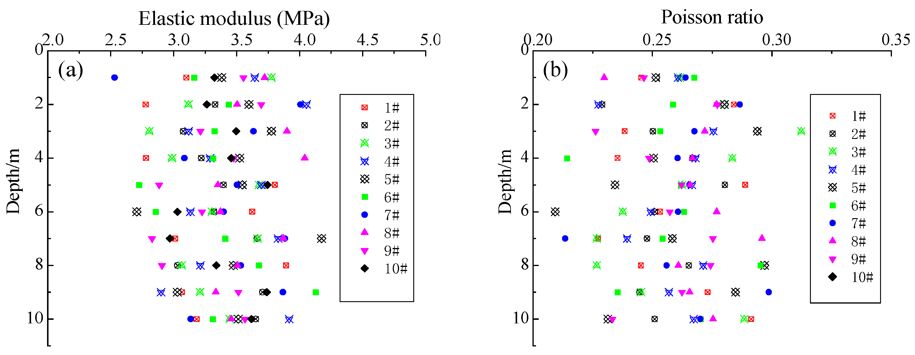
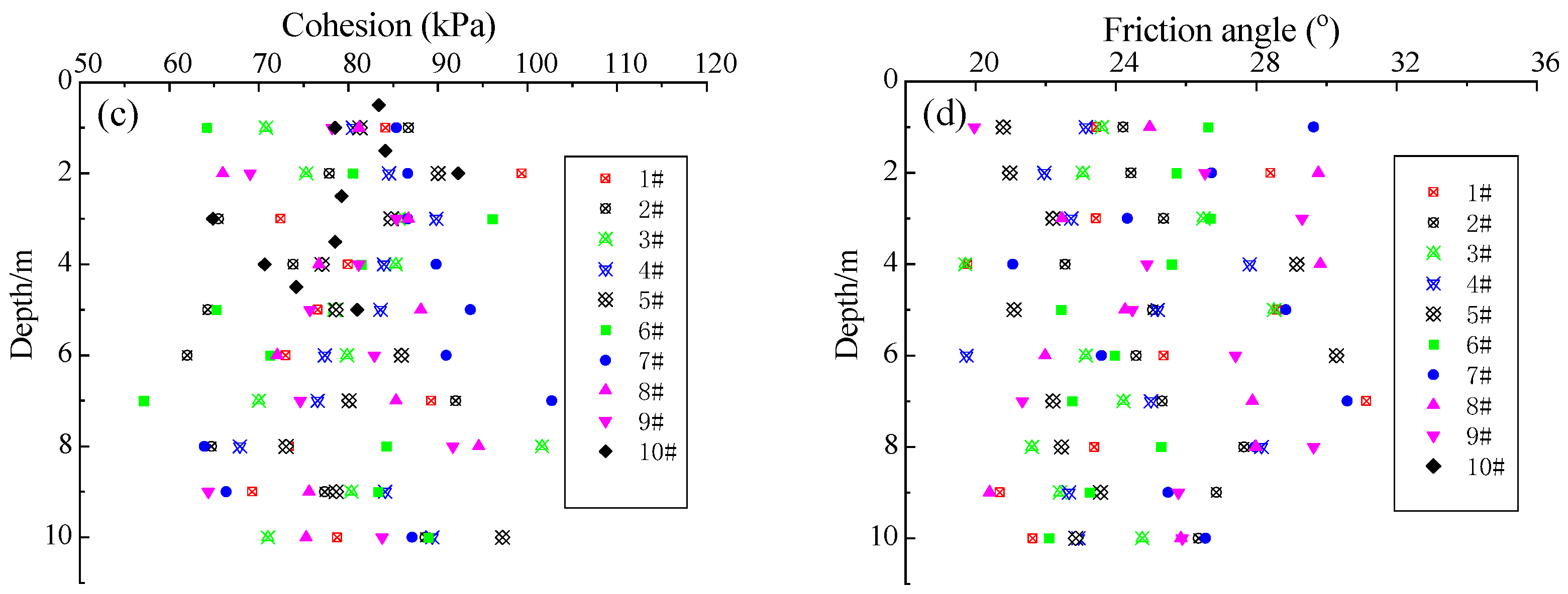
2.1. Generation Method of Limited Sample Data

Geological and soil conditions can be highly complex and heterogeneous. Limited data may result from challenges in accurately characterizing the subsurface layers, especially in regions with diverse lithology and soil types. Conducting comprehensive geotechnical investigations involves significant costs. Budget limitations may constrain the extent and depth of field explorations, leading to a reduced number of test points and limited data coverage [31]. Copula theory finds application in geotechnical engineering, specifically in modeling the complex dependencies among various soil and rock parameters. In subsurface investigations, understanding the joint distribution of factors like soil strength, permeability, and consolidation is crucial for an accurate risk assessment and design. Copulas allow engineers to capture and model the intricate relationships between geotechnical variables, providing insight into their joint behavior without making assumptions about individual distributions. This is particularly valuable in scenarios where traditional methods may oversimplify or overlook the complexities of soil behavior [32]. In slope stability analysis, for example, copulas can help characterize the joint probability of factors contributing to failure, such as soil cohesion, friction angle, and groundwater conditions. Similarly, in foundation design, copula theory aids in assessing the combined influence of parameters like bearing capacity and settlement.

Multivariate copula theory is a statistical framework used to model and analyze the joint distribution of multiple random variables, emphasizing the dependence structure while allowing for flexibility in capturing complex relationships. In the context of multivariate copulas, the emphasis is on understanding how variables co-move or co-vary without being restricted by specific marginal distributions. The theory assumes the independence of marginal distributions, enabling the separation of the marginal behaviors from the dependence structure. This separation allows practitioners to model various types of dependencies, including positive, negative, and tail dependencies, making multivariate copulas particularly useful in fields like finance, environmental science, and reliability analysis [33,34]. Multivariate copulas can be classified into different families, such as Archimedean and Elliptical copulas, each offering unique ways to model dependencies. According to copula theory, if F₁(x₁), F₂(x₂), ···, F_n(x_n) are the marginal distribution functions of the desired n-dimensional parameters, then there must be a copula function which can be expressed as the n-dimensional joint distribution function (JDF) F(x₁, x_2, ···, x_n):

$$G\left(x_1,x_2,\cdots ,x_n\right)=C\left(F_1\left(x_1\right),F_2\left(x_2\right),\cdots ,F_n\left(x_n\right)\right)=C\left(u_1,u_2,\cdots u_n\right)$$

(1)

The corresponding probability density function (PDF) can be written as:

$$f\left(x_1,x_2,\cdots ,x_n\right)=f_1\left(x_1\right)f_2\left(x_2\right)\cdots f_n\left(x_n\right)D\left(F_1\left(x_1\right),F_2\left(x_2\right),\cdots ,F_n\left(x_n\right);\theta \right)$$

(2)

where f_n(x_n) is the PDF of the variable x_n; D(·) is the PDF of C; and θ is the copula parameter.

Spearman rank correlation coefficient defines the correlation between variables through the consistency of the rank between two variables, and its definition can be expressed as follows: if (x₁₁,x₂₁) and (x₁₂,x₂₂) are two sets of observations of random variables (X₁,X₂), if (x₁₁,x₂₁)(x₁₂,x₂₂) > 0, the two sets of observations are consistent, while the opposite is inconsistent. Consider (X₁, X₂) two independent identical distribution vector (X′₁, X′₂) and (X″₁, X″₂); if P [(X₁ − X′₁) (X₂ − X″₂) > 0] says they are a consistent probability and P [(X₁ − X′₁) (X₂ − X″₂) < 0] says they are not a consistent probability, then the Spearman rank correlation coefficient γ is defined as the difference between the probability of consistency and the probability of inconsistency between a random vector and any independent equally distributed vector in this direction:

$$\gamma =3P\left[\left(X_1-{X_1}^{\prime }\right)\left(X_2-{X_2}^{\prime \prime }\right)>0\right]-P\left[\left(X_1-{X_1}^{\prime }\right)\left(X_2-{X_2}^{\prime \prime }\right)<0\right]$$

(3)

Since the Spearman rank correlation coefficient represents the rank consistency of any independent same distribution vector with the sample population or distribution population, the correlation of the Spearman rank correlation coefficient is closer to the population than that of a Kendall rank correlation coefficient. At the same time, the relationship between the rank correlation coefficient γ of Spearman and the parameter θ of the copula function is as follows:

$$\gamma =12{\displaystyle {\int }_0^1{\displaystyle {\int }_0^{1}C\left(u_1,u_2;\theta \right)}}d{u}_{1}d{u}_2-3$$

(4)

The γ can be obtained by the Pearson correlation coefficient of the probability value of the edge distribution of the parameter. The computational relationship can be expressed as:

$$\gamma =\rho \left(F_1\left(X_1\right),F_2\left(X_2\right)\right)$$

(5)

According to Equations (1)–(5), the JDF and PDF of the sample data for the cohesive soil layer induced by undercrossing tunnel excavation can be constructed.

Bootstrap is a resampling technique used for statistical inference, providing a robust method to estimate the sampling distribution of a statistic. It involves creating multiple datasets from sampling with replacement from the original data. This process generates pseudo-populations that mimic the underlying distribution of the observed data [35,36]. The key principle is to approximate the sampling distribution of a statistic by repeatedly drawing samples from the observed data. This allows for the calculation of standard errors, confidence intervals, and other statistical measures without relying on parametric assumptions. In essence, bootstrapping leverages the observed data to simulate a multitude of hypothetical datasets, enabling a more comprehensive understanding of the variability inherent in the sample. It is particularly valuable when the underlying distribution is unknown or complex, providing a versatile tool for statistical analysis and hypothesis testing. The bootstrap sample simulation method mainly includes the following three steps:

Step 1: Sampling with Replacement. Begin by randomly selecting ‘n’ observations from the original dataset, allowing for replacement. In this step, each observation has the potential to be picked multiple times or not at all. The goal is to create a resampled dataset of the same size as the original.

Step 2: Statistic Calculation: Compute the desired statistic (e.g., mean, median, standard deviation) for the newly created resampled dataset. This statistic serves as an estimate for the parameter of interest.

Step 3: Repeat and Aggregate: Repeat the sampling with replacement and statistic calculation process a large number of times. This repetition generates a collection of bootstrap samples and their corresponding statistics. The aggregated results provide insights into the distribution of the statistic of interest.

These three steps are fundamental to the bootstrap method, allowing researchers and statisticians to simulate the variability of a statistic. The method is particularly useful when analytical methods may be challenging or when the underlying population distribution is not well known. The resulting bootstrap distribution provides valuable information for constructing confidence intervals and understanding the uncertainty associated with the estimated statistic.

Based on the above three steps, the subsample with the same distribution of the limited data for the soil layer in the adjacent construction area can be constructed.

2.2. Characterization Process of Spatial Heterogeneity

Soil heterogeneity refers to the variation or diversity in soil properties within a given area or volume. These properties may include factors such as texture, composition, structure, moisture content, and nutrient levels [37]. In other words, soil heterogeneity indicates that different parts of the soil exhibit different characteristics. This variability can occur at various scales, ranging from small micro-environments within a single soil profile to larger spatial scales across a landscape. Factors contributing to soil heterogeneity include geological processes, weathering, biological activity, and human influence such as land use and management practices. Geotechnical engineering considers spatial heterogeneity when assessing the stability and load-bearing capacity of soil structures. Variations in clay properties can lead to differential settlement, affecting the performance of foundations, roads, and other infrastructure projects [38,39]. Random field methods in geotechnical engineering are employed to quantify the spatial variability. In this approach, soil characteristics like shear strength, permeability, and settlement are considered as random fields, acknowledging their spatial distribution across a site. The process involves modeling these parameters as stochastic functions, capturing their variability over space. To describe spatial variability, statistical tools such as variogram analysis and covariance functions are utilized. Variograms illustrate the spatial correlation structure of soil properties, depicting how they change with distance. Random field methods incorporate these variograms to simulate and predict the spatial distribution of soil parameters. The outcome is a probabilistic representation of the subsurface, allowing engineers to assess uncertainties and design structures that account for the inherent variability in soil behavior. By integrating random field methods, geotechnical engineers gain a comprehensive understanding of the complex and heterogeneous nature of soils. This facilitates more accurate risk assessments, reliability analyses, and ultimately leads to safer and more robust designs in geotechnical projects.

The random field model proposed by Vanmarcke considers the soil layer as statistically uniform and the spatial distribution of soil properties as random fields. The essence of this model is to simulate soil profiles with continuous stationary random fields, depict the autocorrelation of geotechnical materials with autocorrelation functions (or autocorrelation distances), and establish the variance calculation method for the transition from the point characteristics obtained from test data to the spatial average characteristics. The statistical properties of random field can be expressed by its finite dimensional joint distribution function or probability density. However, it is often difficult to determine the distribution function or probability density in practical problems. The key parameters mainly include mean function, variance function, correlation function, covariance function, and correlation coefficient. In this paper, the elastic modulus, Poisson ratio, cohesion, and friction angle of the cohesive soil layer in the proximity area is simulated as four independent random fields (e₁, e₂, e₃, e₄). The mean and variance function of the any parameter random field can be written as:

$$\left.\begin{array}{l}E\left[X(e_i)\right]=const=m_i\\ Var\left[X(e_i)\right]=const={\sigma }_i^2\end{array}\right\}$$

(6)

where m_i is the mean of the parametric random field; σ_i is the standard deviation of the parametric random field.

The autocorrelation function of any parameter random field can be expressed as:

$$R_X(e_i,e_j)=E(X(e_i)X(e_j))=R_X(e_i-e_j)=R_X(\tau )$$

(7)

The cross-correlation function of the two parameter random field can be expressed as:

$$\left.\begin{array}{l}{R}_{XY}(e_i,e_j)=E\left[X(e_i)Y(e_j)\right]=E\left[X(e_i)Y(e_j+\tau )\right]=R_{XY}(\tau )\\ R_{YX}(e_i,e_j)=E\left[Y(e_i)X(e_j)\right]=E\left[Y(e_i)X(e_j+\tau )\right]=R_{YX}(\tau )\end{array}\right\}$$

(8)

The covariance function of the two parameter random field can be expressed as:

$$\left.\begin{array}{l}Co{v}_X(e_i,e_j)=E\{[X(e_i)-m_X(e_i)][X(e_j)-m_X(e_j)]\}=R_X(\tau )-m^2=Co{v}_X(\tau )\\ Co{v}_{XY}(e_1,e_2)=E\{[X(e_i)-m_X(e_i)][Y(e_j)-m_Y(e_j)]\}=R_{XY}(\tau )-m_X{m}_Y=Co{v}_{XY}(\tau )\end{array}\right\}$$

(9)

The correlation coefficient of the two parameter random field can be expressed as:

$$\left.\begin{array}{l}{\rho }_X(e_i,e_j)=\frac{Co{v}_X(e_i,e_j)}{{\sigma }_X^2}=\frac{Co{v}_X(\tau )}{{\sigma }_X^2}={\rho }_X(\tau )\\ {\rho }_{XY}(e_i,e_j)=\frac{Co{v}_{XY}(e_i,e_j)}{{\sigma }_X{\sigma }_Y}=\frac{Co{v}_{XY}(\tau )}{{\sigma }_X{\sigma }_Y}={\rho }_{XY}(\tau )\\ \rho (e_i,e_j)=\frac{R_X(e_i,e_j)}{{\sigma }_X^2}=\frac{R_X(\tau )}{{\sigma }_X^2}=\rho (\tau )\end{array}\right\}$$

(10)

According to Equations (7)–(10), the spatial heterogeneity of the cohesive soil layer in the proximity area can be quantified.

2.3. Calculation Detail of Settlement

To study the stress field and settlement of the cohesive soil layer induced by undercrossing tunnel excavation, the first step is to study the constitutive model and numerical algorithm of the cohesive soil layer in the adjacent construction area. Due to the complexity of the cohesive soil layer in the adjacent construction area, a study of its constitutive model is still in the exploratory stage. Most of the constitutive models that have been constructed are in the experimental and theoretical analysis stage, and generally can only reflect one or two of the shear shrinkage, dilatancy, hardening, and softening characteristics [40,41]. The study object may have shear shrinkage, dilatancy, hardening, and softening local areas at the same time. Therefore, the double-yield surface constitutive model is adopted. The double-yield surface constitutive model for cohesive soils is an advanced geotechnical framework that comprehensively characterizes the intricate behavior of cohesive soils. This model is crucial for simulating the response of soils to various loading conditions. It incorporates two distinct yield surfaces to accurately represent normal and shear loading responses. The primary yield surface is associated with normal loading, while the secondary yield surface corresponds to shear loading. This model integrates the Mohr–Coulomb yield criterion with additional parameters, encompassing aspects like dilation, strain hardening, and anisotropy. It offers a nuanced depiction of soil deformation, shear strength, and stress–strain relationships. Engineers utilize this model to optimize the design of foundations, slopes, and retaining structures, ensuring structural stability in geotechnical projects.

Based on the modified Cambridge model, the yield function of the cohesive soil layer induced by undercrossing tunnel excavation can be expressed as:

$$\ln \left(1+\frac{q^2}{M^{2}p\left(p+p_r\right)}\right)=\ln p_x-\ln p$$

(11)

where p is the mean normal stress; q is the generalized shear stress. M and p_r are two model parameters, their values are $6\sin \phi /\left(3-\sin \phi \right)$ and $c\cot \phi$, respectively.

The iso-directional consolidation test results of cohesive soil are plotted in the coordinate system ε_v-lnp, and the iso-directional consolidation curve can be written as:

$${\epsilon }_v=\phi \left(\ln p\right)$$

(12)

After that, the current yield surface function of the cohesive soil layer induced by undercrossing tunnel excavation can be expressed as:

$$f=\ln \frac{p}{p_0}+\ln \left(1+\frac{q^2}{M^{2}p\left(p+p_r\right)}\right)-{\displaystyle \int \frac{d{\epsilon }_v^p}{{\phi }^{\prime }\left(\ln p\right)-\kappa }}=0$$

(13)

where p₀ is the spherical stress at the current yield surface corresponding to the initial volume strain.

The relationship between the change in material volume strain and the spherical stress during the whole stress path from a shear to critical state under different confining pressure conditions can be obtained by a triaxial compression test. It can be written as:

$${\epsilon }_v=\psi \left(\ln \overline{p}\right)$$

(14)

After that, the refer yield surface function of the cohesive soil layer induced by undercrossing tunnel excavation can be expressed as:

$$f=\ln \frac{\overline{p}}{{\overline{p}}_0}+\ln \left(1+\frac{{\overline{q}}^2}{M^2\overline{p}\left(\overline{p}+p_r\right)}\right)-{\displaystyle \int \frac{d{\epsilon }_v^p}{{\psi }^{\prime }\left(\ln \overline{p}\right)-\kappa }}=0$$

(15)

where p₀ is the spherical stress at the current yield surface corresponding to the initial volume strain.

According to the classical elastic–plastic theory, the total settlement of the cohesive soil layer induced by undercrossing tunnel excavation can be divided into an elastic strain increment and plastic strain increment. The stress–strain relationship can be written as:

$$\left\{d\sigma \right\}={\left[D\right]}^{ep}\left\{d\epsilon \right\}={\left[D\right]}^e\left\{d\epsilon \right\}-\frac{{\left[D\right]}^e\left\{\frac{\mathit{\partial }g}{\mathit{\partial }\sigma }\right\}{\left\{\frac{\mathit{\partial }f}{\mathit{\partial }\sigma }\right\}}^T{\left[D\right]}^e}{A+{\left\{\frac{\mathit{\partial }f}{\mathit{\partial }\sigma }\right\}}^T{\left[D\right]}^e\left\{\frac{\mathit{\partial }g}{\mathit{\partial }\sigma }\right\}}\left\{d\epsilon \right\}$$

(16)

where [D]^e is the elastic constitutive matrix; [D]^ep is the elastic–plastic constitutive matrix; [D]^p is the plastic constitutive matrix. A is the function of hardening parameter; $g$ is the plastic potential function, and $g=f$.

Substituting Equations (13) and (15) into (16), the detailed expression of the stress–strain relationship can be obtained.

Finite Element Method (FEM) plays a crucial role in analyzing foundation deformation. It involves discretizing the complex foundation–soil system into smaller elements to simulate real-world behavior. First, the model gathers geotechnical data to establish material properties and loading conditions [42,43]. It creates a model with finite elements representing the foundation and surrounding soil and applies boundary conditions reflecting actual constraints, including external loads and soil–structure interactions. Using FEM to solve equations describing the behavior of each element, the model provides a comprehensive analysis of deformation patterns. FEM aids in understanding the stress distribution, settlement, and potential failure zones. As well, time-dependent analyses consider factors like consolidation and creep, offering insights into long-term behavior. Then, the model is validated against field measurements for accuracy. Sensitivity analyses explore the impact of varying parameters on deformation predictions. This iterative process refines the model, ensuring a reliable tool for studying and mitigating foundation deformations using the powerful Finite Element Method. For the settlement of the cohesive soil layer induced by undercrossing tunnel excavation, the FE formulae can be written as:

$$\left[K\right]\left\{\Delta \delta \right\}=\left\{\Delta R\right\}$$

(17)

$$\left[K\right]={\displaystyle {\int }_{V^e}{\left[B\right]}^T{\left[D\right]}^e\left[B\right]dV}+{\displaystyle {\int }_{V^p}{\left[B\right]}^T{\left[D\right]}^p\left[B\right]dV}+{\displaystyle {\int }_{V^g}{\left[B\right]}^T{\left[D\right]}^g\left[B\right]dV}$$

(18)

where [K] is the stiffness matrix; {ΔR} is the increment of equivalent nodal forces vector; [B] is the element strain matrix; [D]^g is the transitional matrix.

The FEM for elasto-plastic analysis incorporates material nonlinearity to simulate structural behavior under varying loads. It models plastic deformation, capturing the transition from elastic to plastic response. This method employs a stiffness matrix modification, yielding accurate predictions of plastic strains, stress redistribution, and structural performance under cyclic loading. Therefore, the transitional matrix can be written as:

$${\left[D\right]}^g=m{\left[D\right]}^e+\left(1-m\right){\left[D\right]}^p$$

(19)

$$m=\frac{\mathrm{\Delta }{\sigma }_A}{\mathrm{\Delta }{\sigma }_B}$$

(20)

where $\mathrm{\Delta }{\sigma }_A$ is the equivalent yield stress increment. $\mathrm{\Delta }{\sigma }_B$ is the load step stress increment.

According to Equations (16)–(20), the settlement of the cohesive soil layer induced by undercrossing tunnel excavation can be calculated. The width, height, crown radius, and invert depth of the undercrossing tunnel is 3.8 m, 4.1 m, 2.4 m, and 1.3 m, respectively. Figure 2 shows the statistical characteristics of uncertain settlement characteristics of the cohesive soil layer induced by undercrossing tunnel excavation. It can be seen that the settlement of the cohesive soil layer are discretely distributed. This result is reasonable because of the limited sample data and spatial heterogeneity of the cohesive soil layer.

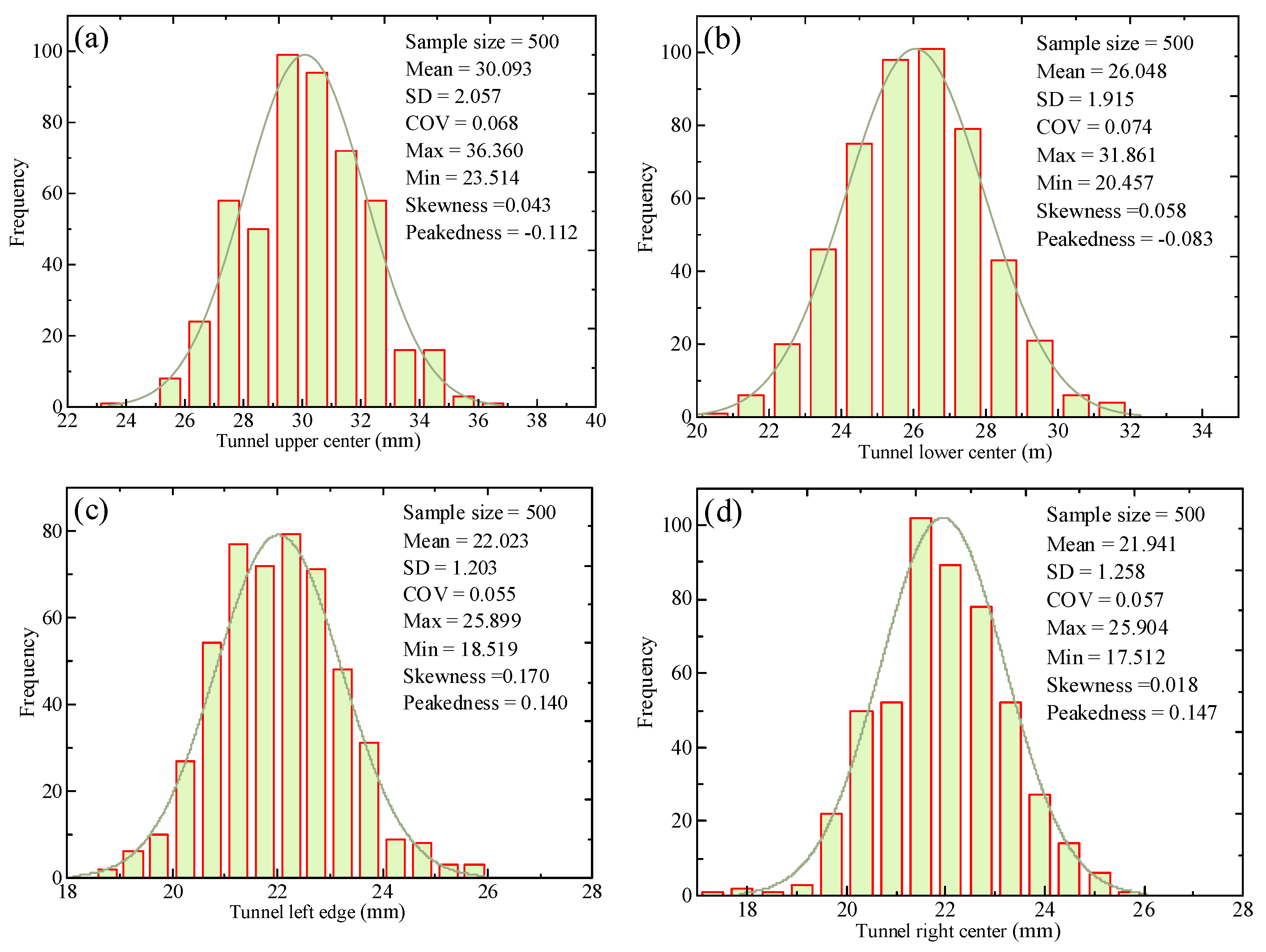
3. Distribution Fitting Test of Different Quantization Process

3.1. Joint Distribution Function

In the field of copula theory, the joint distribution function plays a pivotal role in modeling the dependence structure between multiple random variables. The joint distribution function, often denoted as C₁(u₁, u₂, …, u_n), where u₁, u₂, …, u_n are the individual cumulative distribution functions of the marginal distributions, captures the underlying dependence pattern without specifying the marginal distributions themselves. Copula theory emphasizes the separation of marginal behaviors from the dependence structure, enabling an accurate characterization of complex multivariate relationships. This function is essential in copula modeling as it provides a unified framework to study and model dependence, offering insights into the correlation structure of random variables. By utilizing copulas, researchers and practitioners can better understand and model the joint behavior of variables, facilitating applications in various fields such as risk management and reliability analysis. In this study, five commonly copula joint distribution functions are used. The mathematical expressions are listed in

Table 1. Copula joint distribution function.

Copula	C(u1,u2; θ)	D(u1,u2; θ)	Range of θ
Gaussian	$\begin{array}{l}C\left(u_1,u_2;\mathit{\theta }\right)={\displaystyle {\int }_{-\infty }^{{\mathrm{\Phi }}^{-1}\left(u_1\right)}{\displaystyle {\int }_{-\infty }^{{\mathrm{\Phi }}^{-1}\left(u_2\right)}\frac{1}{2\pi \sqrt{1-{\mathit{\theta }}^2}}}}\\ \times \exp \left[-\frac{{x_1}^2-2\mathit{\theta }{x}_1{x}_2+{x_2}^2}{2\left(1-{\mathit{\theta }}^2\right)}\right]d{x}_{1}d{x}_2\end{array}$	$\begin{array}{l}D\left(u_1,u_2;\mathit{\theta }\right)=\frac{1}{2\sqrt{1-{\mathit{\theta }}^2}}\exp \left(\frac{{{\varsigma }_1}^2-2\mathit{\theta }{\varsigma }_1{\varsigma }_2+{{\varsigma }_2}^2}{2\left(1-{\mathit{\theta }}^2\right)}\right)\\ {\varsigma }_1={\mathrm{\Phi }}^{-1}\left(u_1\right),{\varsigma }_2={\mathrm{\Phi }}^{-1}\left(u_2\right)\end{array}$	[−1,1]
Plackett	$\begin{array}{l}C\left(u_1,u_2;\mathit{\theta }\right)=\frac{S-\sqrt{S^2-4u_1{u}_2\mathit{\theta }\left(\mathit{\theta }-1\right)}}{2\left(\mathit{\theta }-1\right)}\\ S=1+\left(\mathit{\theta }-1\right)\left(u_1+u_2\right)\end{array}$	$\begin{array}{l}D\left(u_1,u_2;\mathit{\theta }\right)=\\ \frac{\mathit{\theta }\left[1+\left(\mathit{\theta }-1\right)\left(u_1+u_2-u_1{u}_2\right)\right]}{\left\{{\left[1+\left(\mathit{\theta }-1\right)\left(u_1+u_2\right)\right]}^2{\left.-4u_1{u}_2\mathit{\theta }\left(\mathit{\theta }-1\right)\right\}}^{3/2}\right.}\end{array}$	$\left(0,\infty \right)\backslash \left\{1\right\}$
Frank	$C\left(u_1,u_2;\mathit{\theta }\right)=-\frac{1}{\mathit{\theta }}\ln \left[1+\frac{\left(e^{-\mathit{\theta }{u}_1}-1\right)\left(e^{-\mathit{\theta }{u}_2}-1\right)}{e^{-\mathit{\theta }}-1}\right]$	$D\left(u_1,u_2;\mathit{\theta }\right)=\frac{-\mathit{\theta }\left(e^{-\mathit{\theta }}-1\right)e^{-\mathit{\theta }\left(u_1+u_2\right)}}{{\left[\left(e^{-\mathit{\theta }}-1\right)+\left(e^{-\mathit{\theta }{u}_1}-1\right)\left(e^{-\mathit{\theta }{u}_2}-1\right)\right]}^2}$	$\left(-\infty ,\infty \right)\backslash \left\{0\right\}$
Clayton	$C\left(u_1,u_2;\mathit{\theta }\right)={\left(u_1^{-\mathit{\theta }},+,u_2^{-\mathit{\theta }}-1\right)}^{-1/\mathit{\theta }}$	$D\left(u_1,u_2;\mathit{\theta }\right)=\left(1+\mathit{\theta }\right){(u_1{u}_2)}^{-\mathit{\theta }-1}{\left({u_1}^{-\mathit{\theta }},+,{u_2}^{-\mathit{\theta }},-,1\right)}^{-2-1/\mathit{\theta }}$	$\left(0,\infty \right)$
No. 16	$\begin{array}{l}C\left(u_1,u_2;\mathit{\theta }\right)=\frac{1}{2}\left(S+\sqrt{S^2+4\mathit{\theta }}\right)\\ S=u_1+u_2-1-\mathit{\theta }\left(\frac{1}{u_1}+\frac{1}{u_2}-1\right)\end{array}$	$\begin{array}{l}D\left(u_1,u_2;\mathit{\theta }\right)=\frac{1}{2}\left(1+\frac{\mathit{\theta }}{{u_1}^2}\right)\left(1+\frac{\mathit{\theta }}{{u_2}^2}\right)S^{-1/2}\\ \times {\left\{-S^{-1}\left[u_1+u_2-1-\mathit{\theta }\left(\frac{1}{u_1}+\frac{1}{u_2}-1\right)\right]\right.}^2\left.+1\right\},\\ S={\left[u_1+u_2-1-\mathit{\theta }\left(\frac{1}{u_1}+\frac{1}{u_2}-1\right)\right]}^2+4\mathit{\theta }\end{array}$	$[0,\infty )$

.

In their application, they unveil the interrelation patterns without specifying individual distributions. This unique feature is crucial in risk assessment and reliability analysis. The core of copula lies in modeling the joint distribution function, separating marginal behaviors from the correlation structure. Archimedean copulas, like Clayton and Gumbel, characterize different dependence shapes. Elliptical copulas, such as Gaussian and t, are popular for capturing various tail dependence scenarios. Understanding copula’s dependence structure involves parameter estimation through methods like maximum likelihood or Kendall’s tau. Goodness-of-fit tests, like Anderson–Darling, ensure the chosen copula accurately reflects the observed data. Copulas facilitate risk modeling by offering flexibility and precision in representing complex relationships, enhancing decision making in diverse fields.

Table 2. Correlation structure function for characterizing the anisotropic spatial variations.

Types	Correlation Structure Function	Parameter Relationship
Exponential	$\rho \left(\mathit{\tau }\right)=\exp \left[-\left(\frac{{\tau }_x}{{\mathit{\theta }}_h}+\frac{{\tau }_y}{{\mathit{\theta }}_v}\right)\right]$	${\mathit{\theta }}_h=\frac{{\delta }_h}{2},{\mathit{\theta }}_v=\frac{{\delta }_v}{2}$
Gaussian	$\rho \left(\mathit{\tau }\right)=\exp \left\{-\left[{\left(\frac{{\tau }_x}{{\mathit{\theta }}_h}\right)}^2+{\left(\frac{{\tau }_y}{{\mathit{\theta }}_v}\right)}^2\right]\right\}$	${\mathit{\theta }}_h=\frac{{\delta }_h}{\sqrt{\pi }},{\mathit{\theta }}_v=\frac{{\delta }_v}{\sqrt{\pi }}$
Second-order regression	$\rho \left(\mathit{\tau }\right)=\exp \left[-\left(\frac{{\tau }_x}{{\mathit{\theta }}_h}+\frac{{\tau }_y}{{\mathit{\theta }}_v}\right)\right]\left[\left(1+\frac{{\tau }_x}{{\mathit{\theta }}_h}\right)\left(1+\frac{{\tau }_y}{{\mathit{\theta }}_v}\right)\right]$	${\mathit{\theta }}_h=\frac{{\delta }_h}{4},{\mathit{\theta }}_v=\frac{{\delta }_v}{4}$
Exponential cosine	$\rho \left(\mathit{\tau }\right)=\exp \left[-\left(\frac{{\tau }_x}{{\mathit{\theta }}_h}+\frac{{\tau }_y}{{\mathit{\theta }}_v}\right)\right]\cos \left(\frac{{\tau }_x}{{\mathit{\theta }}_h}\right)\cos \left(\frac{{\tau }_y}{{\mathit{\theta }}_v}\right)$	${\mathit{\theta }}_h={\delta }_h,{\mathit{\theta }}_v={\delta }_v$
Triangular	$\rho \left(\mathit{\tau }\right)=\left\{\begin{array}{l}\left(1-\frac{{\tau }_x}{{\mathit{\theta }}_h}\right)\left(1-\frac{{\tau }_y}{{\mathit{\theta }}_v}\right)\hspace{0.33em}\hspace{0.33em}\hspace{0.33em}\hspace{0.33em}\hspace{0.33em}\hspace{0.33em}\hspace{0.33em}{\tau }_x\le {\mathit{\theta }}_h,{\tau }_y\le {\mathit{\theta }}_v\\ 0\hspace{0.33em}\hspace{0.33em}\hspace{0.33em}\hspace{0.33em}\hspace{0.33em}\hspace{0.33em}\hspace{0.33em}\hspace{0.33em}\hspace{0.33em}\hspace{0.33em}\hspace{0.33em}\hspace{0.33em}\hspace{0.33em}\hspace{0.33em}\hspace{0.33em}\hspace{0.33em}\hspace{0.33em}\hspace{0.33em}\hspace{0.33em}\hspace{0.33em}\hspace{0.33em}\hspace{0.33em}{\tau }_x>{\mathit{\theta }}_h,{\tau }_y>{\mathit{\theta }}_v\end{array}\right.$	${\mathit{\theta }}_h={\delta }_h,{\mathit{\theta }}_v={\delta }_v$

shows the distribution function and correlation structure of different copula functions. Among the many copula functions, how to select the copula function with the best correlation structure to characterize the clay correlation in the adjacent construction area is a key problem in the parameter joint distribution model. In this section, AIC criterion and BIC criterion are selected to judge the fitting ability.

The AIC criterion can be expressed as follows:

$$\mathrm{AIC}=-2{\displaystyle \sum _{i=1}^N\ln D\left(u_{1i},u_{2i};\mathit{\theta }\right)}+2k$$

(21)

where k is the number of copula function, and (u_1i,u_2i) is defined as:

$$\left\{\begin{array}{c}{u}_{1i}=\frac{\mathrm{rank}\left(x_{1i}\right)}{N+1}\\ u_{2i}=\frac{\mathrm{rank}\left(x_{2i}\right)}{N+1}\end{array}\right.,i=1,2,\cdots ,N$$

(22)

where rank(·) represents the ascending order.

The BIC criterion can be expressed as follows:

$$\mathrm{BIC}=-2{\displaystyle \sum _{i=1}^N\ln D\left(u_{1i},u_{2i};\mathit{\theta }\right)}+k\ln N$$

(23)

Therefore, when the measured data of clay parameters in the adjacent construction area are known, the empirical distribution values are obtained by sorting them in ascending order, and the smallest value obtained is identified by Equation (21) or Equation (23) as the optimal copula function.

3.2. Correlation Structure Function

Random field theory encompasses various crucial functions that contribute to the modeling and analysis of spatial or spatiotemporal data. The covariance function is fundamental, capturing the degree of correlation between random variables at different spatial or temporal locations. It provides insights into the spatial or temporal dependence structure, helping understand how observations influence each other. In spatial statistics, the variogram plays a vital role. It quantifies the variability between observations at distinct spatial distances, offering a measure of spatial heterogeneity. The correlation function, closely linked to the variogram, specifies the strength and direction of spatial dependence, providing essential information for spatial modeling. The random field model can scientifically characterize the objective spatial variability of clay strata in the adjacent construction area. The key parameters required by this method include the mean value, variance, fluctuation range, and related structure of the random field [20,44]. The fluctuation range can be obtained by combining the spatial recurrence method of random fields on the basis of test data. However, the relevant structures of random fields cannot be scientifically determined by measured data or theoretical methods, and the assumptions of relevant structures are generally made in the random analysis of practical engineering, which lacks scientific basis for selection. It is difficult to explain the deviation of analysis results due to the selection of different random field-dependent structures. Therefore, it is necessary to discuss the random field dependent structure of clay formation mechanical parameters and clarify the law of the influence of different correlation structure models on the variability of settlement of the cohesive soil layer.

In general, the correlation structures commonly used to describe the spatial variability of rock and soil strata by using the random field model include exponential type, Gaussian type, second-order regression type, exponential cosine type, and triangular type. The literature [45] gives the mathematical expressions of these five kinds of random field dependent structures. Based on the basic theory and properties of random fields, the mathematical expressions of five commonly used random field-related structures in two-dimensional space are given in this paper, as shown in Table 2.

Table 2 shows that the expression of the two-dimensional random field correlation structure function is directly related to the two-dimensional random field correlation distance, and for different random field correlation structure models, the correlation distance of the random field has different correspondence with the fluctuation range. For example, the fluctuation range of the exponential correlation function in each direction is twice the correlation distance, the fluctuation range of the Gaussian correlation function in each direction is times the correlation distance, the fluctuation range of the second-order regression correlation function in each direction is four times the correlation distance, and the fluctuation range of cosine and triangular correlation function in each direction is equal to the correlation distance. Therefore, after the fluctuation range is obtained from the test data, the specific expressions of five commonly used random field-related structures can be listed in two-dimensional space to provide key parameters for random analysis.

3.3. Fitting Test Process

Distribution fitting tests are crucial in statistical analysis for assessing the appropriateness of a theoretical probability distribution in representing observed data. The process involves several key steps [46,47]. Initially, a hypothesized distribution is selected based on the characteristics of the underlying population. Following this, the observed data is collected, ensuring its relevance to the phenomenon under this study. The parameters of the chosen distribution are then estimated from the data using techniques like Maximum Likelihood Estimation (MLE). A test statistic is selected based on the distribution and nature of the data; common choices include the Kolmogorov–Smirnov statistic or the Anderson–Darling statistic. The next step involves calculating the chosen test statistic. Critical values are determined based on a chosen significance level, establishing a threshold for a satisfactory fit. The hypothesis test is then performed. If the test statistic exceeds the critical value, the null hypothesis is rejected, indicating a poor fit between the observed and hypothesized distributions. The results are interpreted in the context of the study, guiding decisions on whether the selected distribution adequately represents the data. If the fit is deemed inadequate, adjustments can be made by exploring alternative distributions or modifying parameters. This iterative process continues until a satisfactory fit is achieved, ensuring that the chosen theoretical distribution accurately reflects the characteristics of the observed data.

According to uncertain settlement analysis, the settlement deformation samples of the cohesive soil layer induced by undercrossing tunnel excavation can be obtained. It can be seen that each random simulation can obtain a sample of the settlement deformation of the cohesive soil layer induced by undercrossing tunnel excavation, and the distribution fitting test of the sample value is carried out before the reliability evaluation. Due to the large amount of data and limited space, the settlement of the tunnel’s upper center and lower center were selected as examples to conduct the distribution fitting test. Based on a maximum likelihood method and the sample values of stochastic settlement characteristics (Figure 2), mean settlement of the tunnel upper center is 30.093 mm, and standard deviation is 2.057 mm. After stochastic simulation 10,000 times, the maximum is 36.277 mm while the minimum is 23.825 cm. The interval [23.825, 36.277] of 10,000 samples is divided into 10 non-overlapping small intervals. The absolute frequency, frequency, and cumulative frequency are calculated, respectively, and the results are shown in

Table 3. Frequency distribution of settlement for tunnel upper center.

Number	Group (Ti−1, Ti]	Absolute Frequency Fi	Frequency Fi/N	Cumulative Frequency
1	(23.825, 25.070]	15	0.0015	0.0644
2	(25.070, 26.315]	111	0.0111
3	(26.315, 27.560]	518	0.0518
4	(27.560, 28.806]	1496	0.1496	0.214
5	(28.806, 30.051]	2644	0.2644	0.4784
6	(30.051, 31.296]	2718	0.2718	0.7502
7	(31.296, 32.541]	1702	0.1702	0.9204
8	(32.541, 33.786]	647	0.0647	0.9204 + 0.0796 = 1
9	(33.786, 35.031]	136	0.0136
10	(35.031, 36.277]	13	0.0013

.

Further, the frequency f_i/n < 0.05 was combined and finally divided into six groups. According to the statistical theory, the frequency can be described as:

$$p_i=\mathrm{\Phi }\left(\frac{t_i-\mu }{\sigma }\right)-\mathrm{\Phi }\left(\frac{t_{i-1}-\mu }{\sigma }\right)$$

(24)

The computed parameters of the chi-square distribution (Χ²) can be obtained. The results are shown in

Table 4. Computation sheet (Χ²) of settlement for tunnel upper center.

Number	Group (ti−1, ti]	Absolute Frequency fi	Frequency pi	npi	(fi − npi)2/npi
1	(−∞, 30.913]	644	0.0662	661.93	0.4857
2	(30.913, 31.687]	1496	0.1532	1531.60	0.8275
3	(31.687, 32.461]	2644	0.2665	2664.90	0.1639
4	(32.461, 33.235]	2718	0.2723	2722.70	0.0081
5	(33.235, 34.010]	1702	0.1656	1656.20	1.2665
6	(34.010, +∞]	796	0.0763	762.62	1.4610
Total		10,000	1.0000	10,000	4.2128

.

From Table 4, Χ² = 4.2128. It is less than Χ²_0.10(3). Therefore, the settlement of tunnel upper center follows a normal distribution with a significance level of 0.1.

Based on the maximum likelihood method and the sample values of stochastic settlement characteristics, the mean settlement of the tunnel’s lower center is 26.048 mm and standard deviation is 1.915 mm. After stochastic simulation is performed 10,000 times, the maximum is 21.752 mm while the minimum is 30.832 mm. The interval [21.752, 30.832] of 10,000 samples is divided into 10 non-overlapping small intervals. The absolute frequency, frequency, and cumulative frequency are calculated, respectively, and the results are shown in

Table 5. Frequency distribution of settlement for tunnel lower center.

Number	Group (ti−1, ti]	Absolute Frequency fi	Frequency fi/n	Cumulative Frequency
1	(21.752, 22.660]	15	0.0015	0.0755
2	[22.660, 23.568]	121	0.0121
3	[23.568, 24.476]	619	0.0619
4	[24.476, 25.384]	1902	0.1902	0.2657
5	[25.384, 26.292]	3011	0.3011	0.5668
6	[26.292, 27.200]	2649	0.2649	0.8317
7	[27.200, 28.108]	1314	0.1314	0.9631
8	[28.108, 29.016]	316	0.0316	0.9631 + 0.0369 = 1
9	[29.016, 29.924]	47	0.0047
10	[29.924, 30.832]	6	0.0006

.

Further, the frequency f_i/n < 0.05 was combined and finally divided into six groups. According to the Equation (24), the computed parameters of the chi-square distribution (Χ²) can be obtained. The results are shown in

Table 6. Computation sheet (Χ²) of settlement for tunnel lower center.

Number	Group (ti−1, ti]	Absolute Frequency fi	Frequency pi	npi	(fi − npi)2/npi
1	(−∞, 24.476]	755	0.0769	769.00	0.2549
2	(24.476, 25.384]	1902	0.1898	1898.00	0.0084
3	(25.384, 26.292]	3011	0.3050	3050.00	0.4987
4	(26.292, 27.200]	2649	0.2658	2658.00	0.0305
5	(27.200, 28.108]	1314	0.1256	1256.00	2.6783
6	(28.108, +∞]	369	0.0376	376.00	0.1303
Total		10,000	1.0000	10,000	3.6011

.

From Table 6, Χ² = 3.6011. It is less than Χ²_0.10(3). Therefore, the settlement of the tunnel’s lower center follows a normal distribution with a significance level of 0.1.

4. Reliability Analysis and Risk Assessment

4.1. Reliability Function

A geotechnical engineering reliability analysis focuses on assessing the probability of structures or systems performing satisfactorily under varying soil conditions and loads. This entails employing reliability functions, such as the probability density function, cumulative distribution function (CDF), and hazard rate function, to model the behavior of geotechnical systems over time. These functions allow engineers to quantify the likelihood of failure or performance degradation, enabling informed decision making in design, construction, and maintenance. By integrating probabilistic methods like Monte Carlo simulation, geotechnical engineers can better understand uncertainties, optimize designs, and mitigate risks associated with soil variability, ground movement, and foundation stability, ultimately ensuring the reliability and resilience of civil engineering projects in diverse geological environments. The Monte Carlo simulation method in geotechnical engineering involves probabilistically assessing uncertainties related to soil properties, ground conditions, and structural stability. By generating numerous random samples within the defined probability distributions, this approach enables engineers to simulate a wide range of potential scenarios, including soil strength variations, ground settlement, and slope stability. Through iterative simulations and statistical analysis, the Monte Carlo method aids in estimating the probability of failure, assessing risk, and optimizing design parameters, thereby enhancing the reliability and safety of geotechnical structures and infrastructure projects.

Based on the Monte Carlo calculation method and distribution fitting test results, normal distribution can be used to characterize the tunnel uncertainty deformation. According to the limiting equation of state $F_X\left(X_1,X_2,\cdot \cdot \cdot ,X_n\right)-S=0$, the Monte Carlo simulation method is used to generate a set of random numbers conforming to the normal distribution of state variables X₁,X₂, …,X_n. By plugging these random numbers into the state function $Z=F_X\left(X_1,X_2,\cdot \cdot \cdot ,X_n\right)-S$, a random number corresponding to the state function can be obtained. A random number of the N state functions is generated in the same way. If M of the random numbers of N state functions are less than or equal to zero, when N is large enough, the frequency at this time approximates the probability according to the law of large numbers. In geotechnical engineering, reliability functions assess the probability of soil-related structures performing satisfactorily over time, aiding in design optimization and risk assessment. Therefore, the reliability function for settlement of the cohesive soil layer induced by undercrossing tunnel excavation can be defined as:

$$\beta =p\left\{F_X\left(X_1,X_2,\cdot \cdot \cdot ,X_n\right)-S\le 0\right\}=\frac{M}{N}$$

(25)

where S is the permissible value; β is the reliability index.

4.2. Failure Probability

In geotechnical engineering, failure encompasses the inability of soil or rock structures to perform their intended function, leading to compromised safety, stability, or serviceability. Failure can manifest as excessive settlement, slope instability, foundation settlement, or structural collapse, posing risks to infrastructure, property, and human lives. To comprehensively assess the risks associated with geotechnical failures, engineers employ probability analysis methods. These methods involve quantifying the likelihood of failure and its potential consequences through probabilistic modeling and statistical techniques. Deterministic approaches, which rely on precise input parameters and assumptions, are often complemented by probabilistic methods to account for uncertainties inherent in geotechnical systems. Probabilistic modeling considers variations in soil properties, loading conditions, environmental factors, and construction processes to estimate the probability of failure. Advanced techniques such as the Monte Carlo simulation generate multiple scenarios by sampling from probability distributions of input parameters. These simulations simulate the behavior of geotechnical systems under different conditions, allowing engineers to evaluate the likelihood and consequences of failure across a range of scenarios. By integrating probability analysis into geotechnical engineering practices, engineers can make informed decisions regarding design, construction, and risk management. This proactive approach helps to identify potential failure modes, optimize designs to mitigate risks, and enhance the resilience of geotechnical structures against uncertain conditions. In summary, geotechnical failure encompasses various forms of structural inadequacy, and probability analysis methods enable engineers to quantify the likelihood of failure and its potential impacts, thereby enhancing the safety, reliability, and performance of geotechnical infrastructure.

Reliability is a measure of the probability that a system, device, or component will function properly within a specific time frame. It is usually expressed as a percentage or decimal, with values ranging from 0 to 1. The higher the reliability, the less likely the corresponding system or equipment is to fail, and the higher the working stability. Failure probability refers to the probability that a system, device, or component will fail within a certain period of time. The probability of failure can also be expressed as a percentage or decimal and ranges from 0 to 1. The failure probability is inversely proportional to the reliability; that is, the smaller the failure probability, the higher the reliability. The failure probability is inversely proportional to the reliability, that is, the smaller the failure probability, the higher the reliability, and the sum of the two is 1. Based on the above analysis of the permissible value and reliability index, the failure probability for settlement of the cohesive soil layer induced by undercrossing tunnel excavation can be defined as:

$$\psi =1-\beta$$

(26)

Therefore, according to the analytical method of uncertain settlement characteristics, the distribution fitting test of different quantization process, reliability function and failure probability, the reliability value, and failure probability induced by undercrossing tunnel excavation can be analyzed and predicted.

5. Results and Analyses

In this part the reliability index and failure probability of uncertain settlement characteristics for different locations (tunnel upper center, tunnel lower center, tunnel left edge, and tunnel right edge) are calculated and analyzed. The effects of the copula structure and correlation parameter on the reliability indicators are evaluated, respectively.

5.1. Reliability Indicators at Different Locations

Subway tunnel deformations at the top and bottom significantly impact reliability. Top deformations, such as roof collapses or cracks, pose risks of structural failure and water ingress, leading to service disruptions and safety hazards. Bottom deformations, like settlement or subsidence, threaten track alignment and stability, potentially causing derailments or structural damage. The reliability of subway tunnel deformations at the top and bottom is influenced by various factors. Geological conditions, construction quality, and environmental changes affect both top and bottom deformations. Water infiltration, ground stability, and nearby excavation activities contribute to top deformations like cracks and collapses. Bottom deformations, such as settlement or subsidence, are influenced by soil properties, groundwater levels, and construction techniques. Effective drainage systems, reinforced tunnel linings, and regular maintenance mitigate these risks, ensuring the reliability of subway tunnel infrastructure.

Table 7. Reliability index and failure probability of tunnel upper and lower center.

Depth/m	Tunnel Upper Center		Tunnel Lower Center
	Reliability Index/β	Failure Probability/ψ	Reliability Index/β	Failure Probability/ψ
1.0	94.16%	5.84%	95.25%	4.75%
2.0	94.32%	5.68%	95.05%	4.95%
3.0	94.54%	5.46%	95.04%	4.96%
4.0	94.32%	5.68%	95.62%	4.38%
5.0	94.88%	5.12%	96.27%	3.73%
6.0	95.29%	4.71%	95.87%	4.13%
7.0	95.12%	4.88%	96.61%	3.39%
8.0	95.59%	4.41%	96.94%	3.06%
9.0	95.43%	4.57%	96.91%	3.09%
10.0	95.69%	4.31%	96.61%	3.39%

shows the result of a reliability index and failure probability for the tunnel upper and lower center. It can be seen that for the uncertain settlement characteristics of the tunnel upper center, the most likely failure location is 1.0 m depth, the maximum failure probability is 5.84%, and the overall average failure probability is 5.07%. Obviously, this calculation result is reasonable because the excavation of the subway tunnel has a greater influence on the near tunnel wall. It can be seen that for the uncertain settlement characteristics of the tunnel’s lower center, the most likely failure location is 3.0 m depth, the maximum failure probability is 4.96%, and the overall average failure probability is 3.98%. The failure probability is higher at the tunnel upper center than at the tunnel lower center. Therefore, we should pay more attention to the stability of the tunnel upper center. Some necessary subsidence deformation monitoring for the tunnel upper center can effectively reduce the risk of failure.

The reliability of subway tunnel sidewall deformations is crucial for infrastructure integrity. Factors influencing reliability include geological composition, construction methods, and external forces. Poor soil stability, improper excavation techniques, and nearby construction activities may lead to sidewall deformations such as bulges or cracks. Additionally, water infiltration, temperature fluctuations, and seismic events can exacerbate these deformations. Robust engineering designs, including reinforced tunnel linings and ground support systems, help mitigate risks. Regular inspections, advanced monitoring technologies, and prompt maintenance interventions are essential for addressing emerging deformations and ensuring the reliability of subway tunnel sidewalls.

Table 8. Reliability index and failure probability of tunnel left and right edge.

Depth/m	Tunnel Left Center		Tunnel Right Center
	Reliability Index/β	Failure Probability/ψ	Reliability Index/β	Failure Probability/ψ
1.0	96.41%	3.59%	95.39%	4.61%
2.0	96.39%	3.61%	95.35%	4.65%
3.0	96.58%	3.42%	95.37%	4.63%
4.0	96.84%	3.16%	96.09%	3.91%
5.0	97.38%	2.62%	96.21%	3.79%
6.0	97.44%	2.56%	96.33%	3.67%
7.0	97.28%	2.72%	97.01%	2.99%
8.0	97.32%	2.68%	97.13%	2.87%
9.0	97.31%	2.69%	97.08%	2.92%
10.0	98.13%	1.87%	98.67%	1.33%

shows the result of the reliability index and failure probability for the tunnel left and right center. It can be seen that for the uncertain settlement characteristics of the tunnel left center, the most likely failure location is 2.0 m depth, the maximum failure probability is 3.61%, and the overall average failure probability is 2.89%. For the uncertain settlement characteristics of the tunnel right center, the most likely failure location is still 2.0 m depth, the maximum failure probability is 4.65%, and the overall average failure probability is 3.54%. The most vulnerable position of the left and right side walls of the tunnel is not the surface, perhaps due to the soft soil at the depth of 2 m. In addition, the failure probability is higher at the tunnel right center than at the tunnel left center. These results are reasonable because the soil around the tunnel is not uniform. Therefore, we should pay more attention to the stability of the tunnel right center.

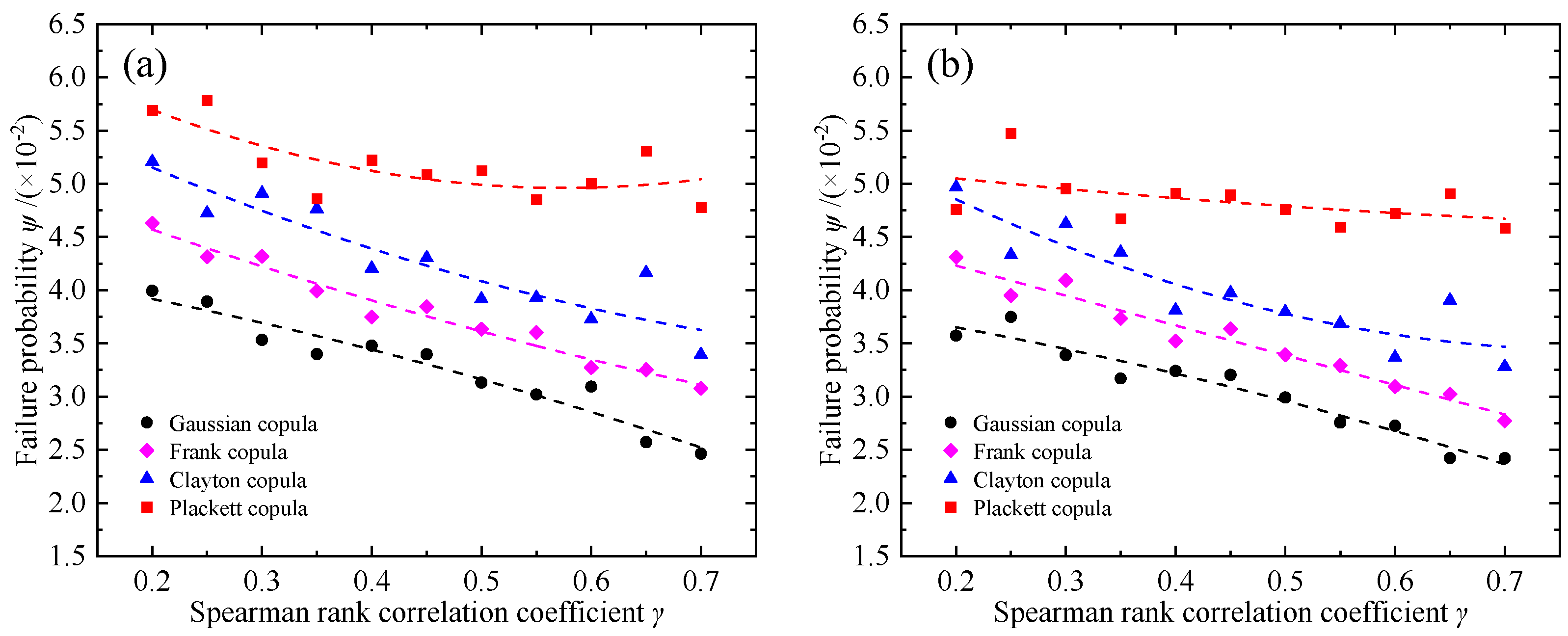
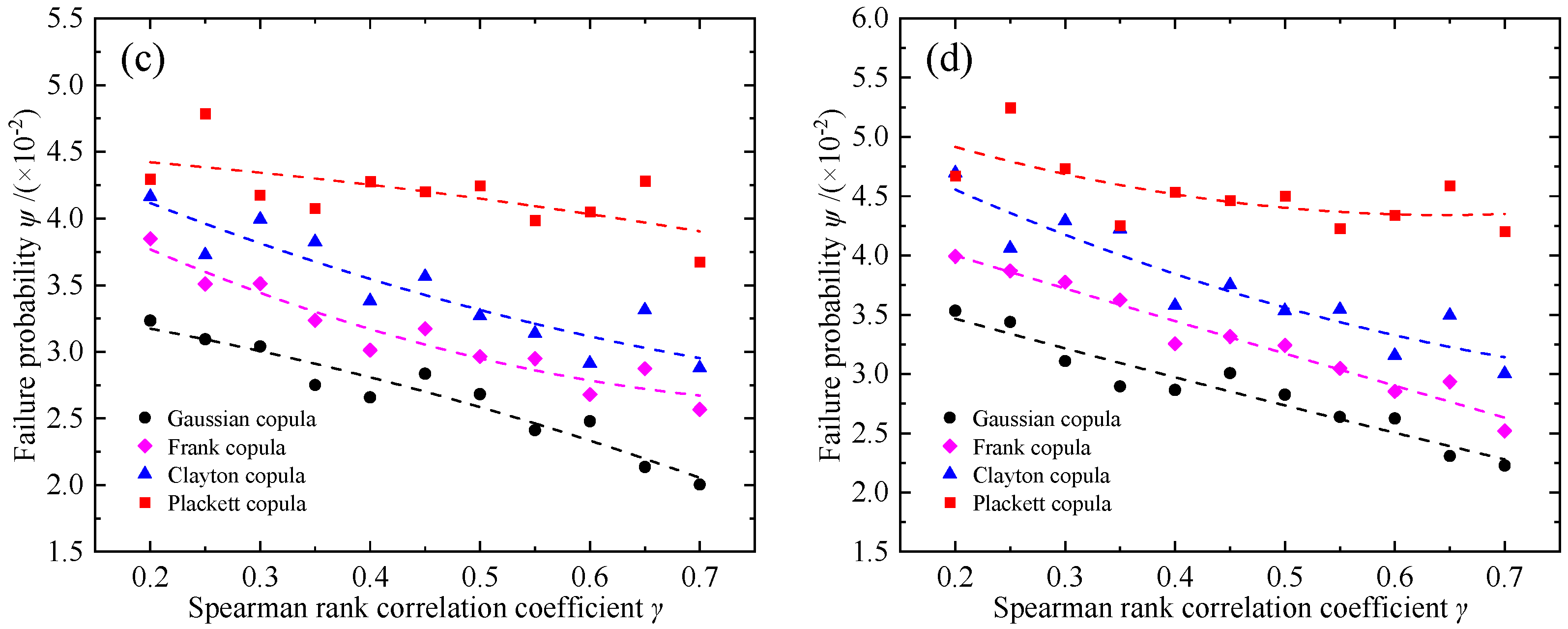
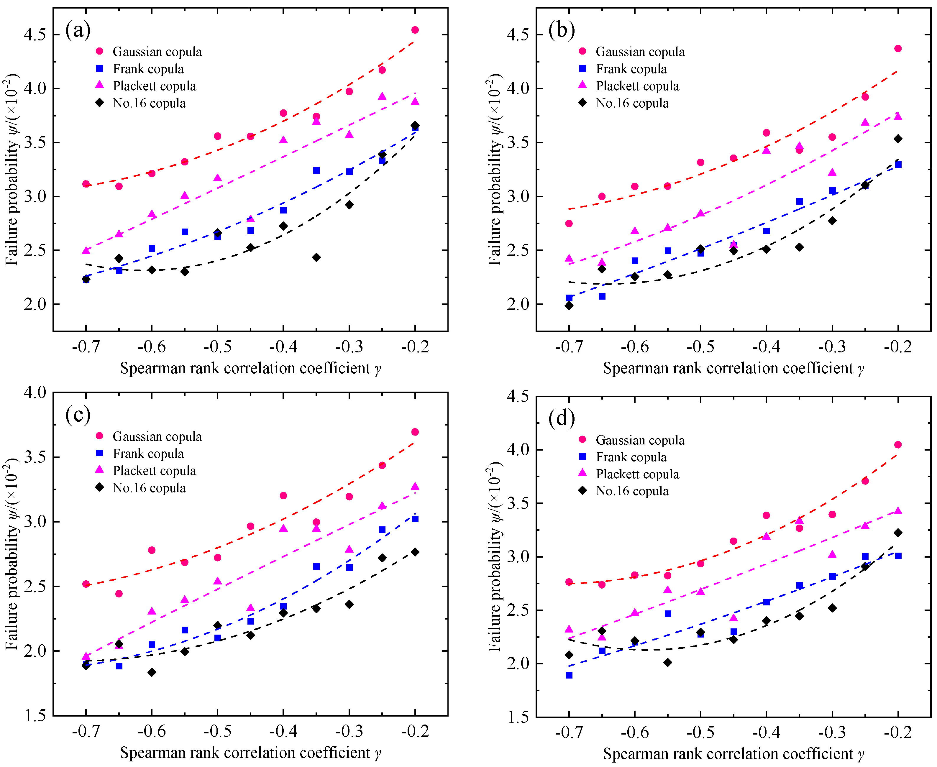
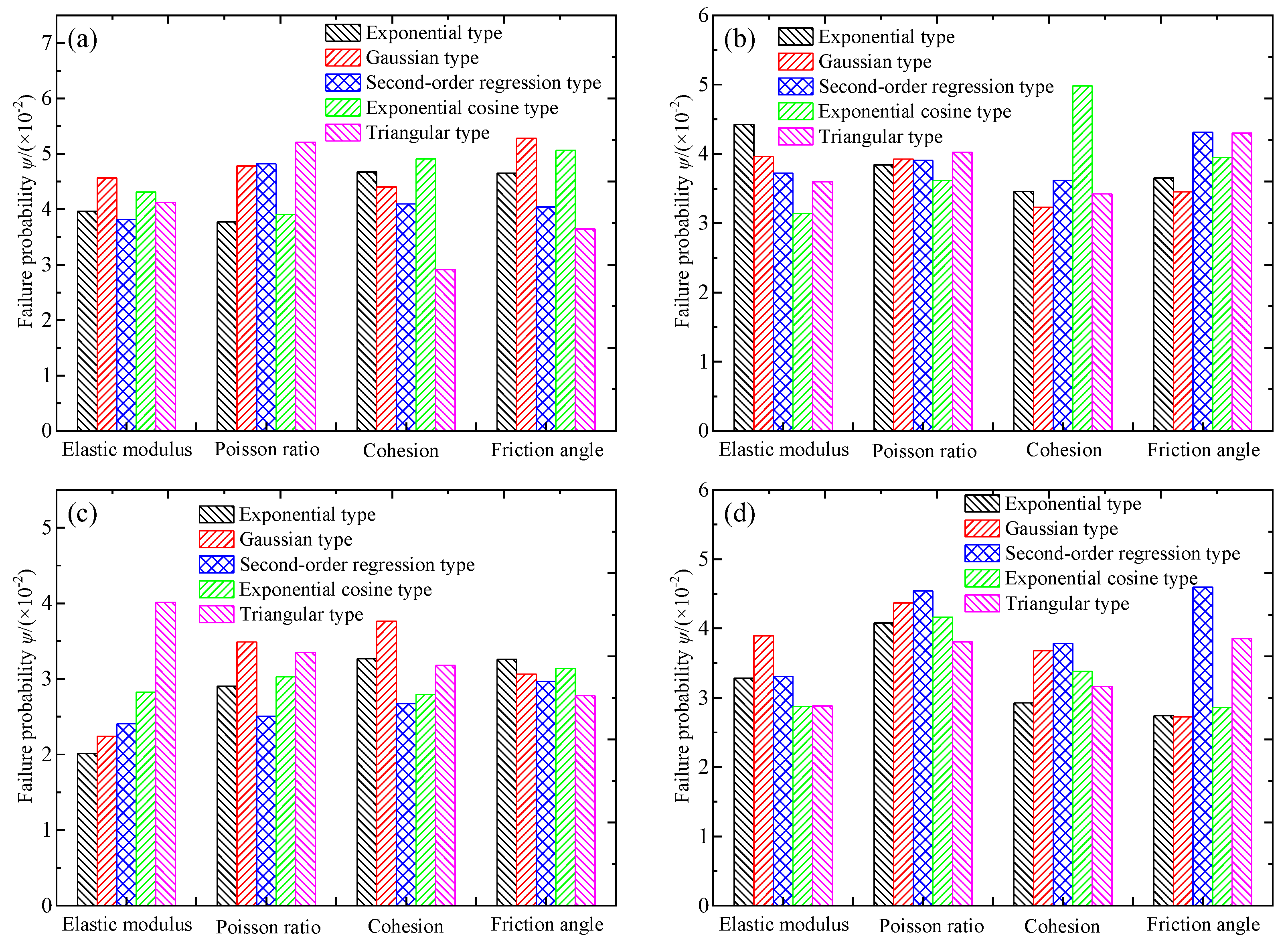
5.2. Effect of Copula Structure

The form of the copula function significantly impacts the reliability analysis. Copulas model the dependence structure between random variables, which is crucial for assessing system reliability. Different copula forms, such as Gaussian, Clayton, or Gumbel, capture varying degrees of dependence, affecting reliability estimation. For instance, Gaussian copulas assume linear dependencies, suitable for systems with symmetric correlations. Clayton copulas represent a stronger dependence in the lower tail, ideal for analyzing extreme events. Gumbel copulas are suitable for modeling tail dependence, important for systems where failures occur concurrently. The choice of copula function influence’s reliability metrics like system failure probabilities or joint exceedance probabilities. Proper selection based on the system’s characteristics ensures an accurate reliability assessment and aids in decision making for risk management and design optimization. Figure 3 shows the result of failure probability of different positive correlation structures. With the increase in the correlation between the positive correlation parameters, the failure probability of the tunnel system decreases. In other words, the failure probability of the tunnel upper center, tunnel lower center, tunnel left edge, and tunnel right edge are reduced. In addition, it can be seen that the failure probability of the tunnel system obtained by simulating positive correlation parameters with different copula functions is obviously different. For different copula structures, the Plackett copula has the greatest effect, while the Gaussian copula has the smallest effect. The error in calculating the system failure probability using different copula structures under different correlation parameters can exceed two times. Therefore, considering the positive correlation of uncertain parameters is essential in settlement induced by undercrossing tunnel excavation.

The form of the copula function significantly impacts reliability analysis. Copulas model the dependence structure between random variables, which is crucial for assessing system reliability. Different copula forms, such as Gaussian, Clayton, or Gumbel, capture varying degrees of dependence, affecting reliability estimation. For instance, Gaussian copulas assume linear dependencies, which is suitable for systems with symmetric correlations. Clayton copulas represent a stronger dependence in the lower tail, ideal for analyzing extreme events. Gumbel copulas are suitable for modeling tail dependence, which is important for systems where failures occur concurrently. The choice of copula function influences the reliability metrics like system failure probabilities or joint exceedance probabilities. Proper selection based on the system’s characteristics ensures accurate reliability assessment and aids in decision making for risk management and design optimization. Figure 4 shows the result of failure probability of different negative correlation structures of copula. With the increase in the correlation between the positive correlation parameters, the failure probability of the tunnel system increases. In other words, the failure probability of the tunnel upper center, tunnel lower center, tunnel left edge, and tunnel right edge are increased. In addition, it can be seen that the failure probability of under system obtained by simulating positive correlation parameters with different copula functions is obviously different. For different copula structures, the Gaussian copula has the greatest effect, while the No.16 copula has the smallest effect. The error in calculating the system failure probability using different copula structures under different correlation parameters can exceed 1.5 times. Therefore, considering the negative correlation of uncertain parameters is essential in settlement induced by undercrossing tunnel excavation. We can only obtain the effect of the copula structure because the spatial variability and correlation of uncertain mechanical parameters for the clay layer are quantified by random fields under incomplete probability data. Selecting the appropriate copula function needs to consider the correlation structure, marginal distributions, dependency structure, model complexity, and model fitting techniques.

5.3. Effect of Correlation Parameter

Different autocorrelation functions within random fields exert varying impacts on the failure probability assessments in geotechnical engineering. Autocorrelation functions describe the spatial correlation between soil properties, crucial for understanding failure mechanisms. A rapidly decaying autocorrelation function signifies a high spatial variability, leading to localized failure modes and potentially elevated failure probabilities in specific areas. Conversely, a slowly decaying autocorrelation function indicates smoother spatial variations, resulting in more gradual failure patterns and potentially lower overall failure probabilities across the site. Moreover, the correlation length associated with autocorrelation functions influences the extent of spatial dependency, directly affecting the spatial distribution of failure probabilities. Understanding these autocorrelation functions enables engineers to better anticipate failure scenarios, optimize risk mitigation strategies, and enhance the reliability of geotechnical designs. The correlation structures commonly used to describe the spatial variability of rock and soil strata by using random field model include exponential type, Gaussian type, second-order regression type, exponential cosine type, and triangular type. Selecting autocorrelation functions depends on soil heterogeneity and failure mechanisms. Rapidly decaying functions suit highly variable soils with localized failure, while slowly decaying functions are ideal for smoother soil variations with gradual failure. In this study, the underground penetration depth of the subway is about 10.5 m, and the soil layer is mainly composed of mixed fill (0~0.5 m), silty clay (0.5~5.0 m), and clay (5.0~10.5 m). Therefore, it is not certain which autocorrelation functions are better. Figure 5 shows the failure probability of the different correlation parameters of random field. From Figure 5a, the maximum probability of failure is 5.28% when considering the elastic modulus of the cohesive soil layer as Gaussian type. The minimum probability of failure is 2.91% when considering the cohesion of the cohesive soil layer as triangular type. As can be seen from Figure 5b, the maximum probability of failure is 4.98% when considering the cohesion of the cohesive soil layer as exponential cosine type. The minimum probability of failure is 3.14% when considering the elastic modulus of the cohesive soil layer as exponential cosine type. From Figure 5c, the maximum probability of failure is 4.01% when considering the elastic modulus of the cohesive soil layer as triangular type. The minimum probability of failure is 2.01% when considering the elastic modulus of cohesive soil layer as exponential type. As can be seen from Figure 5d, the maximum probability of failure is 4.61% when considering the friction angle of the cohesive soil layer as second-order regression type. The minimum probability of failure is 2.73% when considering the friction angle of the cohesive soil layer as Gaussian type. Therefore, different variability parameters and autocorrelation functions have different effects on the failure probability of the cohesive soil layer induced by undercrossing tunnel excavation.

6. Conclusions

In this study, a generation method of limited sample data for the cohesive soil layer in the adjacent construction area is proposed. The spatial variability and correlation of uncertain mechanical parameters for the clay layer are quantified by random fields under incomplete probability data. A calculation method of uncertain settlement for the cohesive soil layer in the adjacent construction area is developed. The distribution fitting tests of settlement characteristics are conducted with different joint distribution functions and correlation structures. A reliability analysis and risk assessment methodology for settlement of the cohesive soil layer is presented. The reliability value and failure probability induced by undercrossing tunnel excavation are analyzed. The main conclusions obtained are as follows:

(1) The bootstrap simulated sampling and random field method can quantify the cohesive soil layer heterogeneity reasonably under limited investigation data. The uncertain settlement is discretely distributed because of the limited sample data and spatial heterogeneity of the cohesive soil layer. The settlement sample of the soil layer around the tunnel follows a normal distribution with a significance level of 0.1.

(2) The excavation of the subway tunnel has a greater influence on the near tunnel wall. The uncertain settlement of the upper center of the tunnel is the largest, and the failure disaster is most likely to occur. The most vulnerable position of the left and right side walls of the tunnel is not the surface. The failure probability is higher at the tunnel right center than at the tunnel left center.

(3) With the increase in the correlation between the positive correlation parameters, the failure probability of the tunnel system decreases. The failure probability of the tunnel system obtained by simulating positive correlation parameters with different copula functions is obviously different. For different copula structures, the Plackett copula has the greatest effect, while the Gaussian copula has the smallest effect.

(4) With the increase in the correlation between the positive correlation parameters, the failure probability of the tunnel system increases. The failure probability of the under system obtained by simulating positive correlation parameters with different copula functions is obviously different. For different copula structures, the Gaussian copula has the greatest effect, while the No.16 copula has the smallest effect.

(5) The correlation structures used to describe the spatial variability of rock and soil strata by using random field model include exponential type, Gaussian type, second-order regression type, exponential cosine type, and triangular type. However, different variability parameters and autocorrelation functions have different effects on the failure probability of the cohesive soil layer induced by undercrossing the tunnel excavation.

Research on subway tunnel construction’s impact on surrounding buildings is pivotal. It enables a comprehensive risk assessment, ensuring structural stability, and minimizing potential damage. Understanding these effects aids urban planning, ensuring infrastructure resilience and public safety. Additionally, it informs construction practices, fostering innovation, and sustainable development. In the future, increased focus on subway tunnel construction reliability and risk control measures is imperative. Enhancing reliability ensures uninterrupted transportation services and public safety. Advanced monitoring technologies and predictive maintenance strategies can prevent potential failures. Moreover, comprehensive risk control measures, such as structural reinforcements and emergency response protocols, mitigate the impact of unforeseen events. Prioritizing research and investment in these areas fosters sustainable urban development and instills public confidence in underground transportation systems, ultimately promoting resilience and enhancing the quality of urban life.

References

1. Yoo, C.; Kim, K. Evaluation of Ground Settlement Induced by Tunneling Construction in Urban Areas. Tunn. Undergr. Space Technol. 2019, 91, 103–116. [Google Scholar]
2. Wei, H.; Wu, H.; Ren, G.; Tang, L.; Feng, K. Energy-based analysis of seismic damage mechanism of multi-anchor piles in tunnel crossing landslide area. Deep Undergr. Sci. Eng. 2023, 2, 245–261. [Google Scholar] [CrossRef]
3. De Sousa, J.R.; Figueiredo, A.D.; Martins, A.I. Influence of Tunneling Construction on Adjacent Structures: A Review. Tunn. Undergr. Space Technol. 2017, 68, 78–89. [Google Scholar]
4. Alnuaim, I.; Abdelgader, H.; Mohammed, K. Assessment of Building Damage Due to Tunnelling-Induced Settlements: Case Study of Riyadh Metro Project. Geotech. Geol. Eng. 2020, 38, 5351–5366. [Google Scholar]
5. Mair, R.J.; Taylor, R.N.; Bracegirdle, A. Analysis of ground movements and ground loss in tunnelling beneath Piccadilly, London. Geotechnique 2005, 55, 605–615. [Google Scholar]
6. Elshafie, M.Z.; Soga, K.; Wright, P.; Mair, R.J. Risk assessment and prediction of ground movements for EPB tunnelling in soft ground. Tunn. Undergr. Space Technol. 2010, 25, 173–184. [Google Scholar]
7. Han, X.; Ye, F.; Han, X.; Ren, C.; Song, J.; Zhao, R. Mechanical responses of underground carriageway structures due to construction of metro tunnels beneath the existing structure: A case study. Deep Undergr. Sci. Eng. 2023. [Google Scholar] [CrossRef]
8. Janas, P.; Mankelow, J.; Hutton, R.; Macdonald, A. Lessons from the construction of the Jubilee Line Extension. Proc. ICE-Eng. Sustain. 2013, 166, 25–32. [Google Scholar]
9. Liu, X.; Lu, H.; Wang, X. Analysis of Building Damage Induced by Subway Tunnel Excavation: A Case Study in Nanjing. Tunn. Undergr. Space Technol. 2015, 47, 145–154. [Google Scholar]
10. Karakus, M.; Su, Y. Geotechnical challenges and monitoring in deep underground construction: The case of Crossrail, London. Tunn. Undergr. Space Technol. 2017, 66, 176–186. [Google Scholar]
11. Jiang, H.; Mu, J.; Zhang, J.; Jiang, Y.; Liu, C.; Zhang, X. Dynamic evolution in mechanical characteristics of complex supporting structures during large section tunnel construction. Deep Undergr. Sci. Eng. 2022, 1, 183–201. [Google Scholar] [CrossRef]
12. Zhu, Y.; Li, J.; Wu, G. Safety analysis of surrounding buildings during subway tunnel construction based on numerical simulation. Tunn. Undergr. Space Technol. 2020, 95, 103140. [Google Scholar]
13. Li, M.; Zhang, Y.; Liu, X.; Zhang, Y. Spatial variability analysis of soil mechanical parameters using sequential Gaussian simulation. Soil Dyn. Earthq. Eng. 2023, 151, 106002. [Google Scholar]
14. Wang, T.; Cao, J.; Pei, X.; Hong, Z.; Liu, Y.; Zhou, G. Research on spatial scale of fluctuation for the uncertain thermal parameters of artificially frozen soil. Sustainability 2022, 14, 16521. [Google Scholar] [CrossRef]
15. Nadimi, S.; Mohajeri, M.; Ghasemi, A. Probabilistic characterization of spatial variability of soil properties using copulas and Bayesian networks. Eng. Geol. 2022, 297, 106575. [Google Scholar]
16. Mendoza-Rivera, A.T.; Kumar, S.; Diez, M. A hybrid data-driven modeling approach for quantifying spatial variability of soil properties in heterogeneous terrains. Comput. Geotech. 2021, 138, 104238. [Google Scholar]
17. Zhang, Y.; Li, W.; Liu, X.; Zhang, Y. Spatial copula-based analysis of soil mechanical parameters variability in a loess hilly region. Catena 2021, 202, 105245. [Google Scholar]
18. Li, W.; Zhang, Y.; Liu, X. Spatial variability and prediction of soil mechanical parameters using geostatistics in a loess hilly region of China. Eng. Geol. 2021, 292, 106292. [Google Scholar]
19. Wang, T.; Zhou, G.; Wang, J.; Zhao, X. Stochastic analysis for the uncertain temperature field of tunnel in cold regions. Tunn. Undergr. Space Technol. 2016, 59, 7–15. [Google Scholar] [CrossRef]
20. Shanahan, P.; Alhajeri, N.S.; Marshall, A.M. Quantification of spatial variability of geotechnical parameters using copulas. Int. J. Geomech. 2020, 20, 04019167. [Google Scholar]
21. Pardo-Igúzquiza, E.; Atkinson, P.M.; Dowd, P.A. Simulation of spatial variability of soil properties using stochastic imaging. Geoderma 2019, 334, 55–66. [Google Scholar]
22. Lizarraga, J.J.; Buscarnera, G. Probabilistic modeling of shallow landslide initiation using regional scale random fields. Landslides 2020, 17, 1979–1988. [Google Scholar] [CrossRef]
23. Wang, T.; Zhou, G.; Wang, J.; Yin, L. Stochastic analysis of uncertainty mechanical characteristics for surrounding rock and lining in cold region tunnels. Cold Reg. Sci. Technol. 2018, 145, 160–168. [Google Scholar] [CrossRef]
24. Ng, T.T.; Goh, A.T.; Tani, K. A novel framework for quantifying spatial variability of soil properties using machine learning techniques. Geoderma 2018, 322, 1–11. [Google Scholar]
25. Zhang, Y.; Li, W.; Liu, X.; Zhang, Y. Joint spatial variability analysis of soil mechanical parameters using copula-based geostatistics. Comput. Geotech. 2019, 107, 139–150. [Google Scholar]
26. Sun, Y.; Wu, J.; Wang, H.; Li, Y. Spatial variability analysis of soil mechanical properties based on the parameter estimation of particle swarm optimization algorithm. Eng. Geol. 2019, 253, 53–62. [Google Scholar]
27. Bulut, R.; Ozcep, F. Comparative analysis of different geostatistical methods for spatial variability of soil properties. Environ. Monit. Assess. 2016, 188, 265. [Google Scholar]
28. Ribeiro, A.I.; Nunes, L.J.; Martins, J.A. Stochastic modeling of spatial variability of soil properties. Environ. Earth Sci. 2015, 73, 1737–1748. [Google Scholar]
29. Hu, J.; Ma, J.; Zhang, L.; Liu, X. Numerical simulation analysis of shield tunnel construction impact on adjacent buildings and ground settlement. Comput. Geotech. 2022, 142, 104505. [Google Scholar]
30. Wang, H.; Zheng, H.; Cai, Y. Ground deformation analysis during shield tunneling construction in soft soil using distributed fiber optic sensing. Tunn. Undergr. Space Technol. 2021, 113, 103715. [Google Scholar]
31. Das, B.S.; Patra, A.K.; Maiti, S. Copula-based geostatistical analysis of spatial variability in soil properties of a tropical acid soil. Environ. Earth Sci. 2014, 73, 1737–1748. [Google Scholar]
32. Zhang, Y.; Liu, X.; Hu, J.; Zhang, Y.; Li, W. Copula-based spatial variability analysis of soil mechanical parameters considering land-use patterns. J. Soils Sediments 2018, 18, 1113–1125. [Google Scholar]
33. Wang, H.; Wu, J.; Sun, Y.; Li, Y. Copula-based spatial variability analysis of soil mechanical properties in the Loess Plateau, China. Catena 2017, 158, 226–234. [Google Scholar]
34. Wu, J.; Wang, H.; Sun, Y.; Li, Y. Copula-based spatial variability analysis of soil mechanical properties considering soil thickness. Geoderma 2017, 295, 12–20. [Google Scholar]
35. Wang, H.; Sun, Y.; Wu, J.; Li, Y. Uncertainty Analysis of Soil Parameters in Foundation Engineering Using Bootstrap Method. Geotech. Test. J. 2023, 46, 20210080. [Google Scholar]
36. Liu, X.F.; Tang, X.S.; Li, D.Q. Efficient Bayesian characterization of cohesion and friction angle of soil using parametric bootstrap method. Bull. Eng. Geol. Environ. 2021, 80, 1809–1828. [Google Scholar] [CrossRef]
37. Zhang, Y.; Liu, X.; Hu, J.; Zhang, Y.; Li, W. Stochastic Analysis of Spatial Heterogeneity of Soil Mechanical Parameters. Geotech. Geol. Eng. 2023, 41, 111–126. [Google Scholar]
38. Wang, T.; Zhou, G.; Chao, D.; Yin, L. Influence of hydration heat on stochastic thermal regime of frozen soil foundation considering spatial variability of thermal parameters. Appl. Therm. Eng. 2018, 142, 1–9. [Google Scholar] [CrossRef]
39. Zhang, Y.; Li, W.; Liu, X.; Zhang, Y. Stochastic Analysis of Spatial Heterogeneity of Soil Mechanical Parameters Using Sequential Gaussian Simulation. Int. J. Geomech. 2019, 19, 04018103. [Google Scholar]
40. Zhang, L.; Wang, H.; Zheng, H. Uncertainty Analysis of Soil Parameters in Geotechnical Engineering Using Bootstrap Method. Int. J. Geomech. 2019, 19, 04018105. [Google Scholar]
41. Liu, S.; Li, X. Evaluation of ground settlement caused by shield tunnel construction in soft soil using a combined numerical and empirical method. Int. J. Geomech. 2020, 20, 04020021. [Google Scholar]
42. Sun, Y.; Wu, J.; Wang, H.; Li, Y. Copula-based spatial variability analysis of soil mechanical properties considering rainfall infiltration. Geoderma 2019, 349, 107–117. [Google Scholar]
43. Wu, J.; Wang, H.; Sun, Y.; Li, Y. Copula-based spatial variability analysis of soil mechanical properties: A case study in the Loess Plateau, China. Eng. Geol. 2018, 235, 91–99. [Google Scholar]
44. Ren, Q.; Zhai, J. Copula-based multivariate analysis of spatial variability in soil parameters. J. Geotech. Geoenviron. Eng. 2018, 144, 04018084. [Google Scholar]
45. Li, D.-Q.; Ding, Y.-N.; Tang, X.-S.; Liu, Y. Probabilistic risk assessment of landslide-induced surges considering the spatial variability of soils. Eng. Geol. 2021, 283, 105976. [Google Scholar] [CrossRef]
46. Xu, Z.; Dai, F. Distribution fitting analysis of rock mass strength parameters based on Markov Chain Monte Carlo method. Eng. Geol. 2023, 293, 106570. [Google Scholar]
47. Li, W.; Zhang, Y.; Liu, X.; Zhang, Y. Evaluation of statistical distributions for modeling soil mechanical properties: A case study in a loess hilly region. Eng. Geol. 2022, 295, 106197. [Google Scholar]
Figure 1. Mechanical parameter of cohesive soil layer of ten different sampling points: (a) Elastic modulus; (b) Poisson ratio; (c) cohesion; (d) friction angle.
Sustainability 16 02356 g001aSustainability 16 02356 g001b
Figure 2. Statistical characteristics of uncertain settlement characteristics of cohesive soil layer: (a) tunnel upper center; (b) tunnel lower center; (c) tunnel left edge; (d) tunnel right edge.
Sustainability 16 02356 g002
Figure 3. Failure probability of positive correlation structure of copula: (a) tunnel upper center; (b) tunnel lower center; (c) tunnel left edge; (d) tunnel right edge.
Sustainability 16 02356 g003aSustainability 16 02356 g003b
Figure 4. Failure probability of negative correlation structure of copula: (a) tunnel upper center; (b) tunnel lower center; (c) tunnel left edge; (d) tunnel right edge.
Sustainability 16 02356 g004
Figure 5. Failure probability of different correlation parameter of random field: (a) tunnel upper center; (b) tunnel lower center; (c) tunnel left edge; (d) tunnel right edge.
Sustainability 16 02356 g005