


Assessment of Groundwater Potential Zones Utilizing Geographic Information System-Based Analytical Hierarchy Process, Vlse Kriterijumska Optimizacija Kompromisno Resenje, and Technique for Order Preference by Similarity to Ideal Solution Methods: A Case Study in Mersin, Türkiye


Abstract
1. Introduction
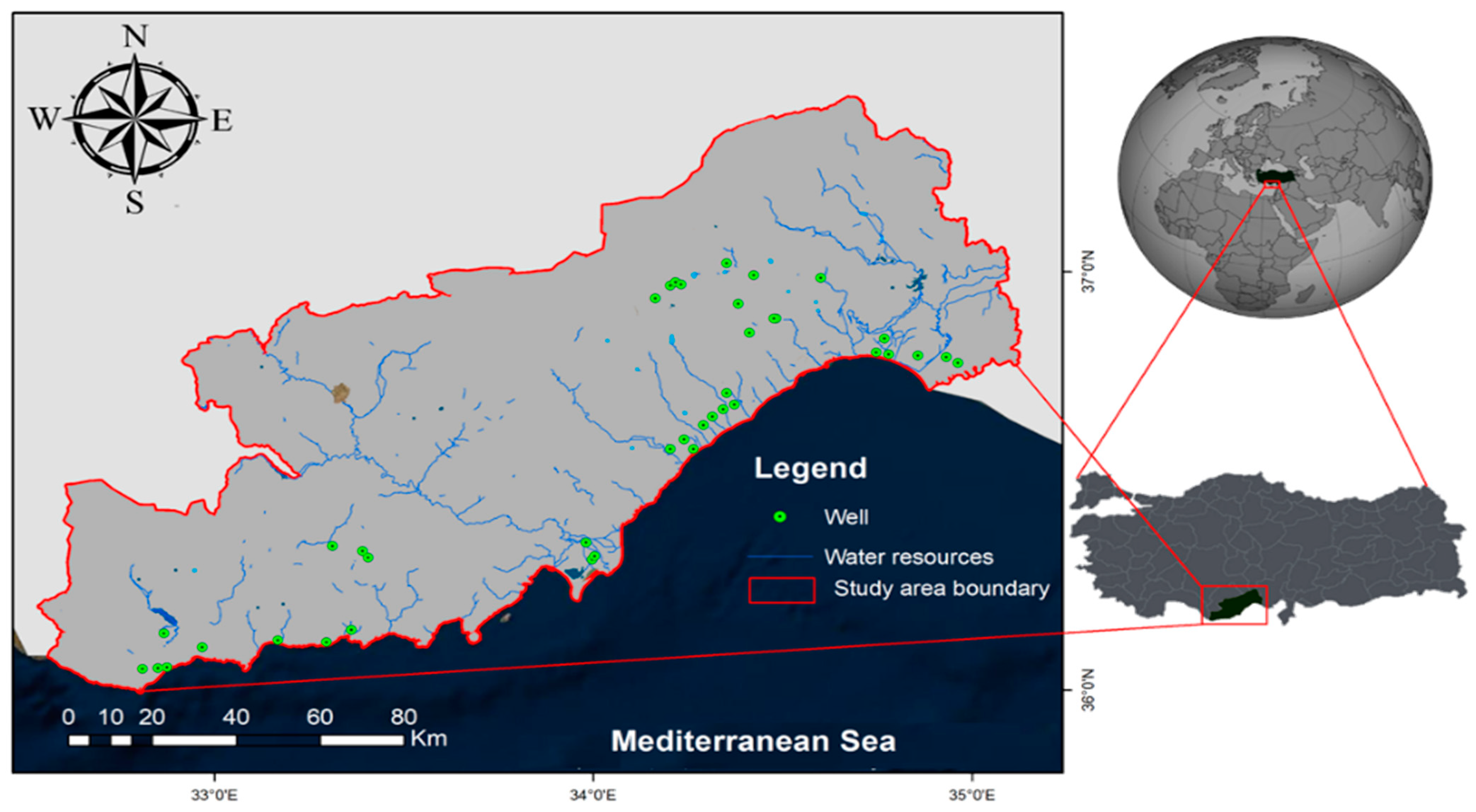
2. Study Area
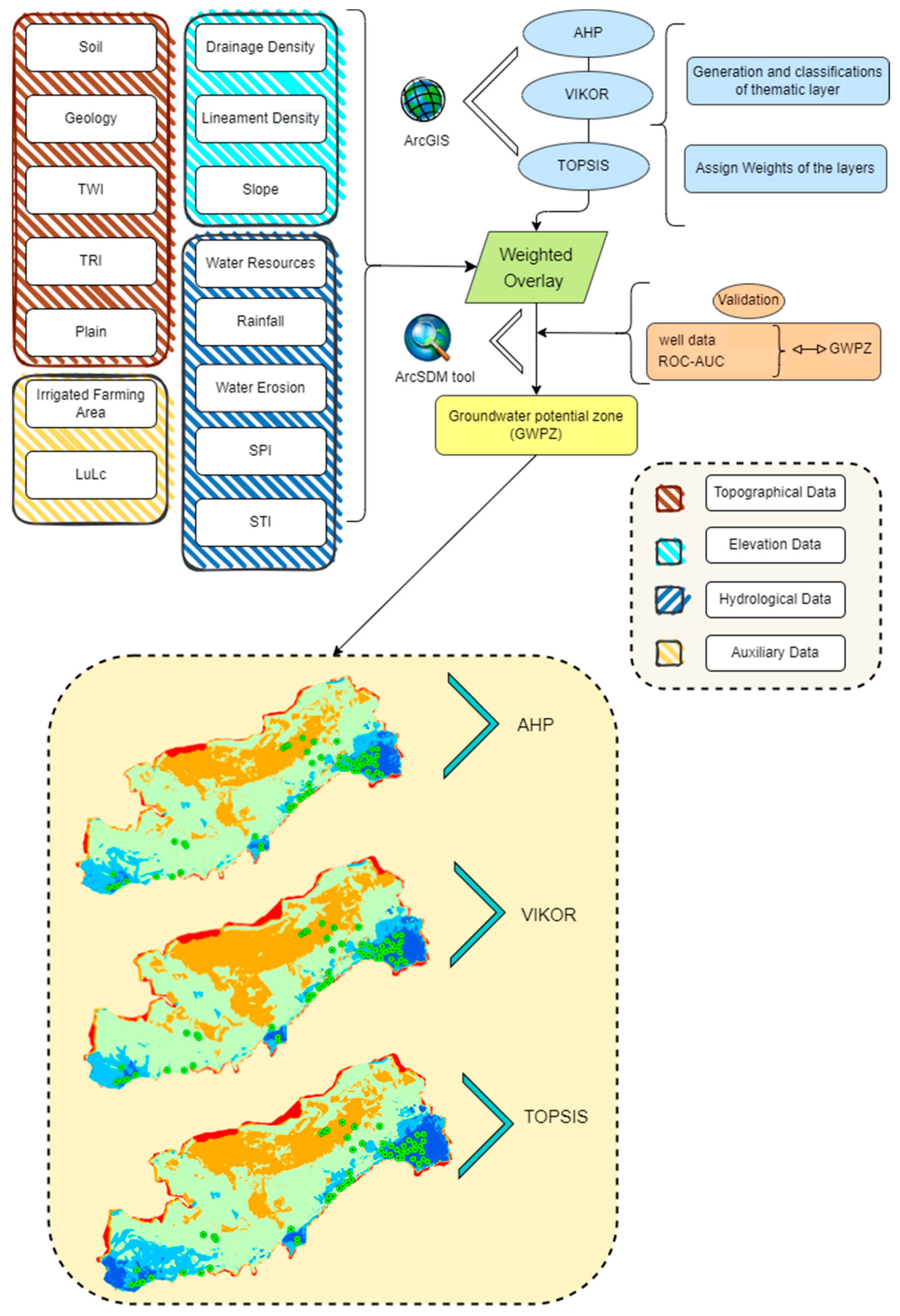
3. Materials and Methods
3.1. Definition of the Thematic Layers
3.1.1. Topographical Data
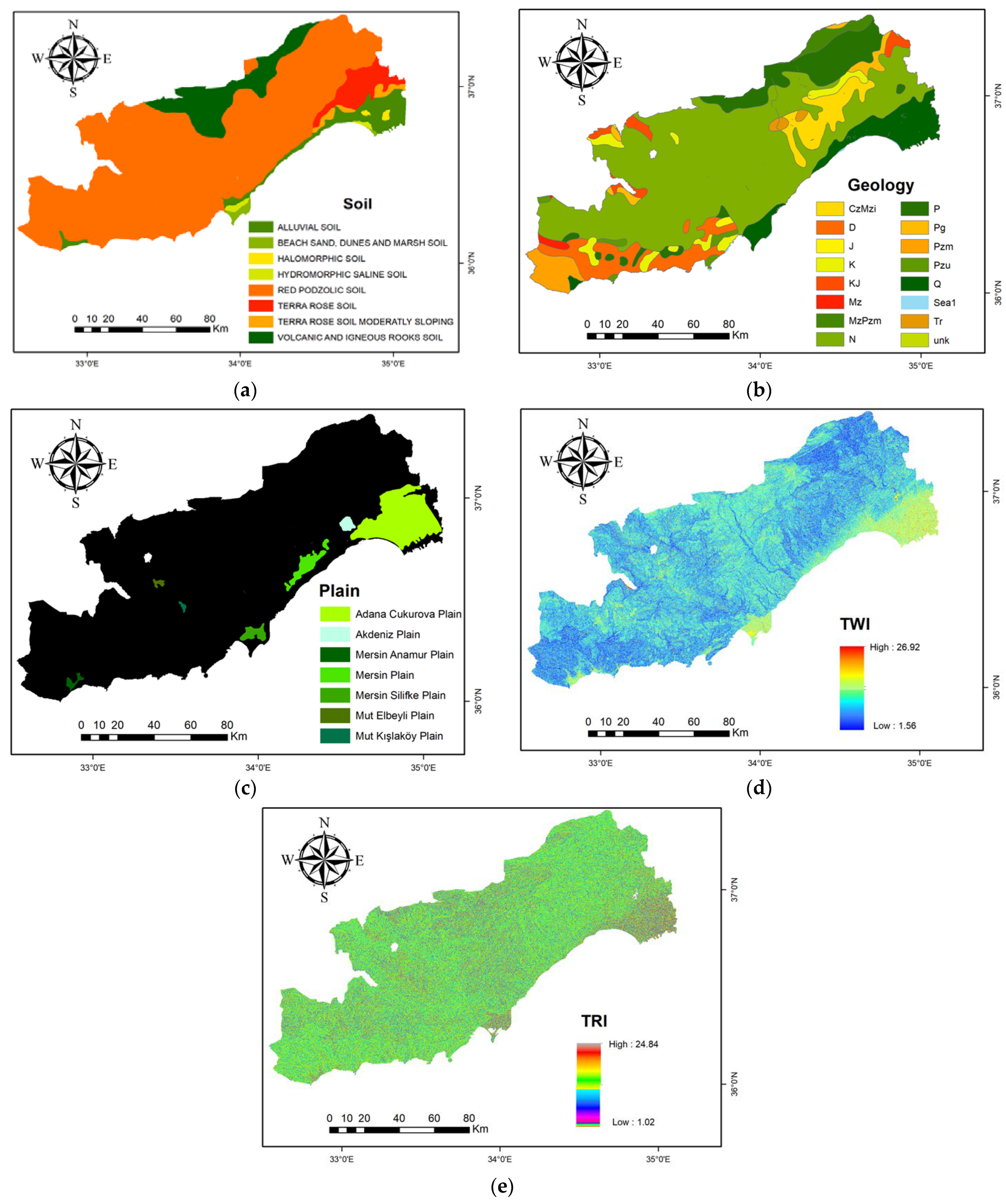
Soil
Geology
Topographic Wetness Index (TWI)
Topographic Roughness Index (TRI)
Plains
3.1.2. Elevation Data
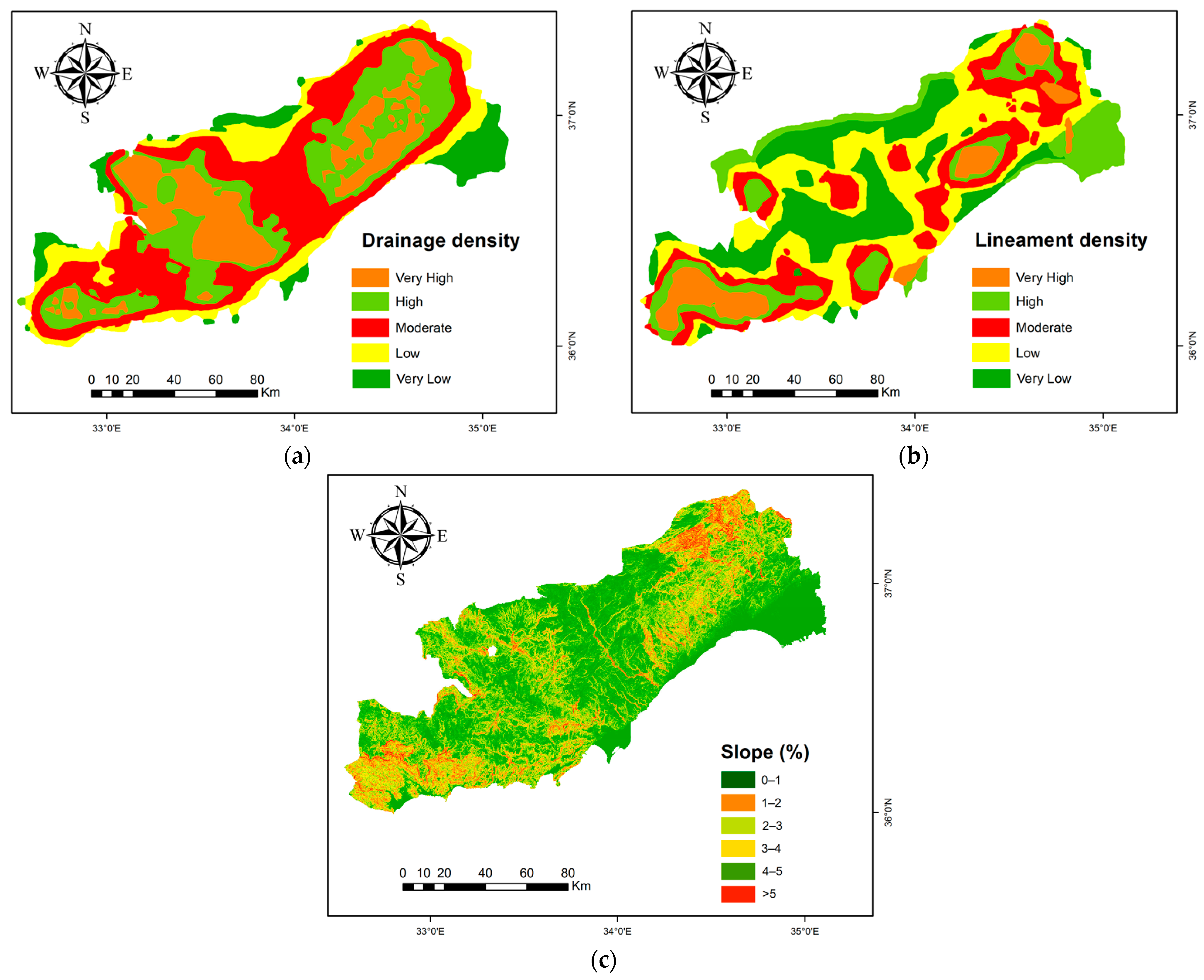
Drainage Density
Lineament Density
Slope
3.1.3. Hydrological Data
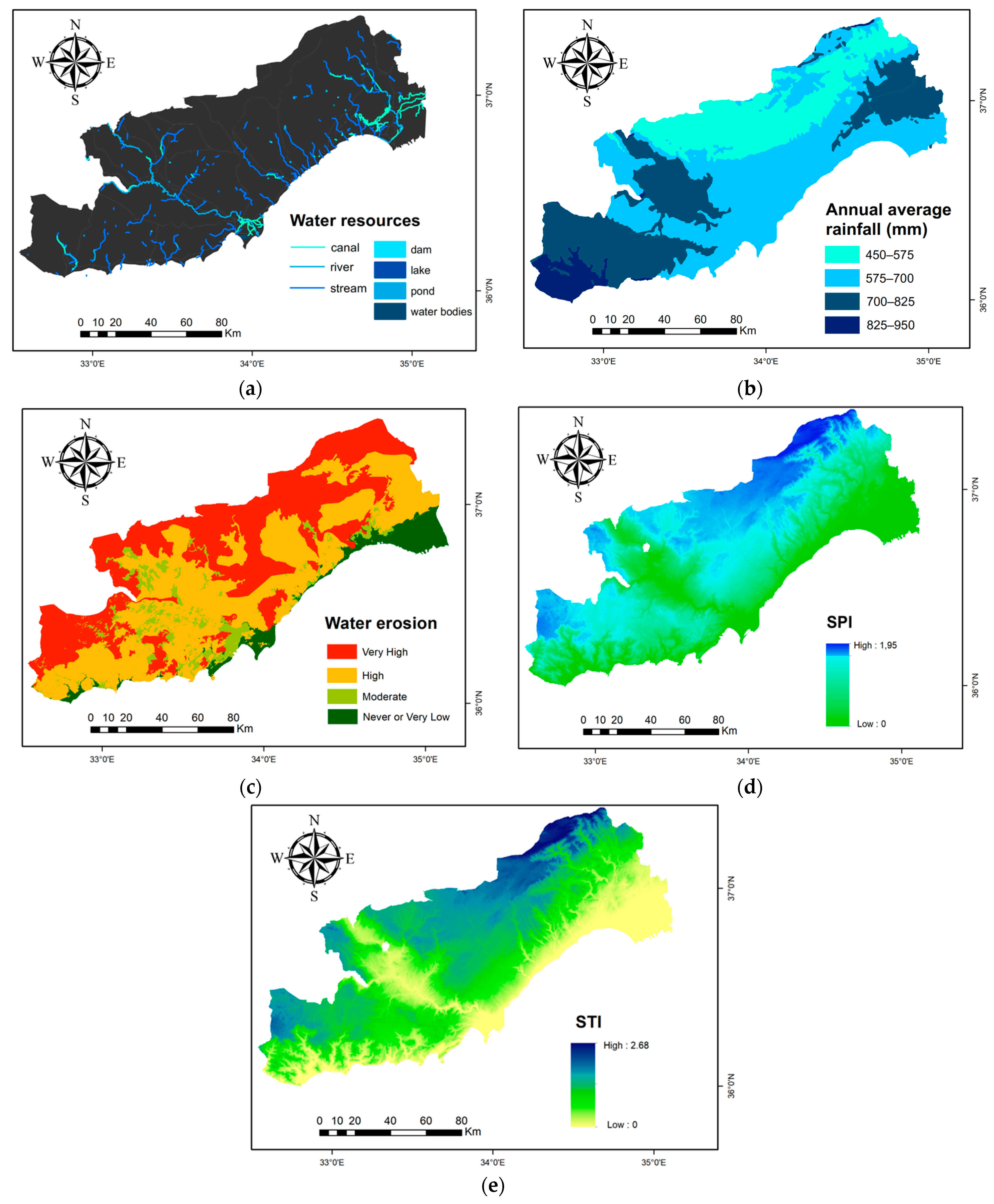
Water Resources
Rainfall
Water Erosion
Stream Power Index (SPI)
Sediment Transport Index (STI)
3.1.4. Auxiliary Data
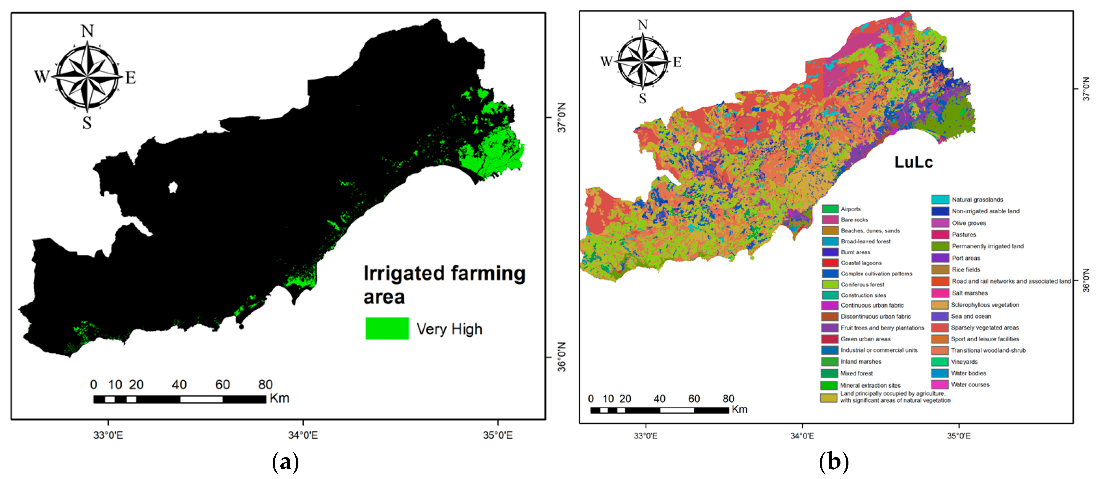
Irrigated Farming Areas
Land Use/Land Cover (LuLc)
3.2. AHP
3.3. VIKOR
3.4. TOPSIS
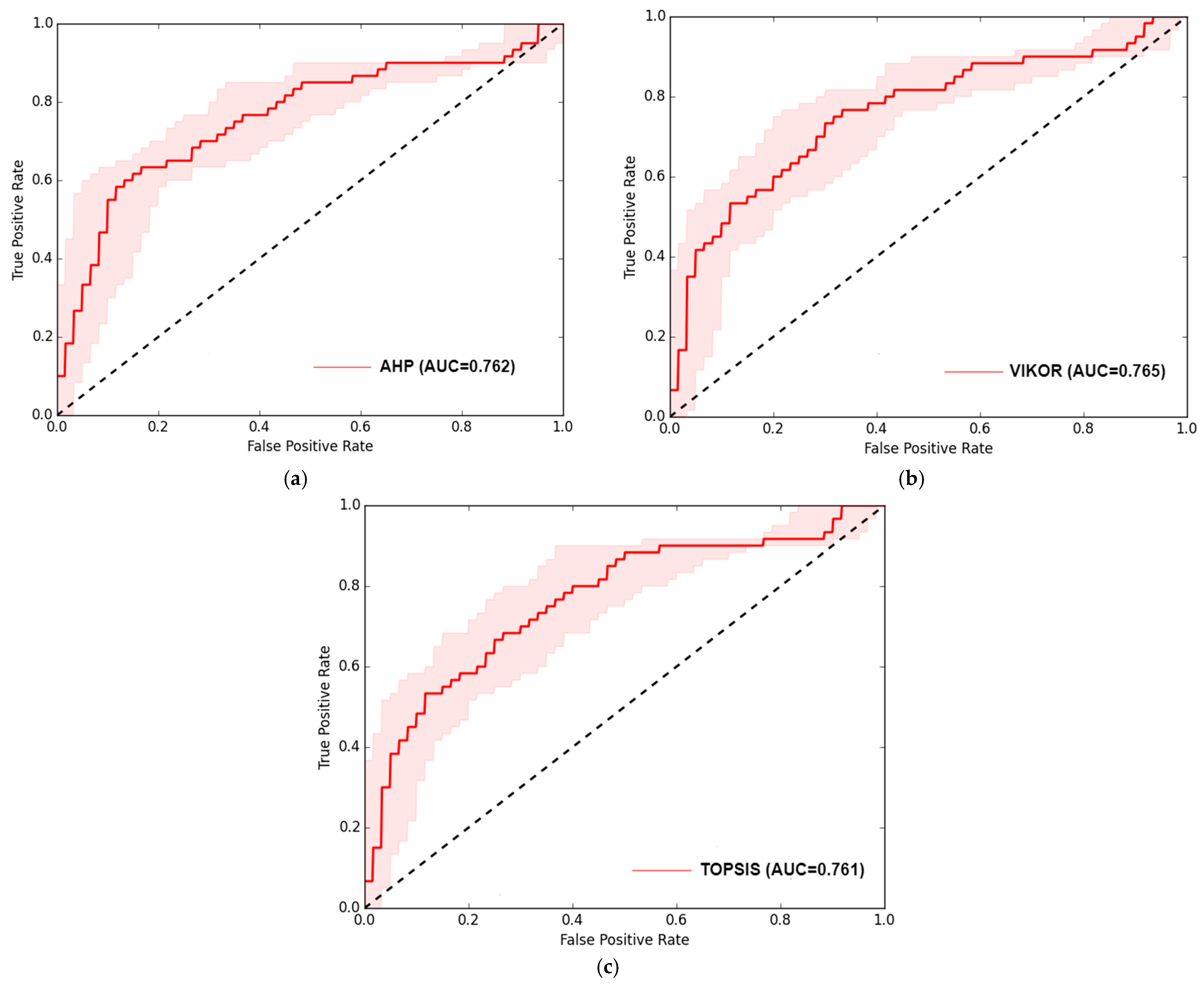
3.5. Validation
4. Results
5. Discussion
6. Conclusions
Author Contributions
Funding
Institutional Review Board Statement
Informed Consent Statement
Data Availability Statement
Conflicts of Interest
References
- Adere, T.H.; Mertens, K.; Maertens, M.; Vranken, L. The impact of land certification and risk preferences on investment in soil and water conservation: Evidence from southern Ethiopia. Land Use Policy 2022, 123, 106406. [Google Scholar] [CrossRef]
- Han, D.; Currell, M.J. Persistent organic pollutants in China’s surface water systems. Sci. Total Environ. 2017, 580, 602–625. [Google Scholar] [CrossRef]
- Kumar, V.; Parihar, R.D.; Sharma, A.; Bakshi, P.; Sidhu, G.P.S.; Bali, A.S.; Kargaouzas, I.; Bhardwaj, R.; Thukral, A.K.; Gyasi-Agyei, Y.; et al. Global evaluation of heavy metal content in surface water bodies: A meta-analysis using heavy metal pollution indices and multivariate statistical analyses. Chemosphere 2019, 236, 124364. [Google Scholar] [CrossRef]
- Dastgerdi, A.S.; Sargolini, M.; Allred, S.B.; Chatrchyan, A.M.; Drescher, M.; DeGeer, C. Climate change risk reduction in cultural landscapes: Insights from Cinque Terre and Waterloo. Land Use Policy 2022, 123, 106359. [Google Scholar] [CrossRef]
- Hutchinson, A.S.; Woodside, G.D.; Herndon, R.L. Increasing the Sustainable Yield of the Orange County Groundwater Basin with Managed Aquifer Recharge. Groundwater 2022, 60, 628–633. [Google Scholar] [CrossRef]
- Moraes-Santos, E.C.; Dias, R.A.; Balestieri, J.A.P. Groundwater and the water-food-energy nexus: The grants for water resources use and its importance and necessity of integrated management. Land Use Policy 2021, 109, 105585. [Google Scholar] [CrossRef]
- Roy, S.; Hazra, S.; Chanda, A.; Das, S. Assessment of groundwater potential zones using multi-criteria decision-making technique: A micro-level case study from red and lateritic zone (RLZ) of West Bengal, India. Sustain. Water Resour. Manag. 2020, 6, 4. [Google Scholar] [CrossRef]
- Tarbuck, E.J.; Lutgens, F.K.; Tasa, D.G. Earth: An Introduction to Physical Geology, 12th ed.; Pearson: London, UK, 2017. [Google Scholar]
- Taylor, R.G.; Scanlon, B.; Döll, P.; Rodell, M.; Van Beek, R.; Wada, Y.; Longuevergne, L.; Leblanc, M.; Famiglietti, J.S.; Edmunds, M.; et al. Ground water and climate change. Nat. Clim. Chang. 2013, 3, 322–329. [Google Scholar] [CrossRef]
- Li, P.; Qian, H.; Wu, J. Conjunctive use of groundwater and surface water to reduce soil salinization in the Yinchuan Plain, North-West China. Int. J. Water Res. Dev. 2018, 34, 337–353. [Google Scholar] [CrossRef]
- MAF. Ministry of agriculture and Forestry (MAF). Available online: https://www.tarimorman.gov.tr/News/5217/325-Facilities-Put-Into-Service-On-The-World-Water-Day (accessed on 20 January 2022).
- Agarwal, R.; Garg, P.K. Remote Sensing and GIS Based Groundwater Potential & Recharge Zones Mapping Using Multi-Criteria Decision Making Technique. Water Resour Manag. 2016, 30, 243–260. [Google Scholar] [CrossRef]
- Saranya, T.; Saravanan, S. Groundwater potential zone mapping using analytical hierarchy process (AHP) and GIS for Kancheepuram District, Tamilnadu, India. Model. Earth Syst. Environ. 2020, 6, 1105–1122. [Google Scholar] [CrossRef]
- Todd, D. Groundwater Hydrology; Wiley: New York, NY, USA, 1980; pp. 111–163. [Google Scholar]
- Bilgilioglu, S.S. Land suitability assessment for Olive cultivation using GIS and multi-criteria decision-making in Mersin City, Turkey. Arab. J. Geosci. 2021, 14, 2434. [Google Scholar] [CrossRef]
- Borah, H.; Deka, S. Exploration of Potential Zones of Groundwater in Jamuna Watershed, Assam, by Applying Multi-influencing Factor Technique. J. Indian Soc. Remote Sens. 2023, 51, 75–91. [Google Scholar] [CrossRef]
- Bozdag, A.; Ertunc, E. Real Property Valuation in the Sample of the City of Niğde through GIS and AHP Method. J. Geomat. 2020, 5, 228–240. [Google Scholar] [CrossRef]
- Dogan, Y.; Yakar, M. GIS and Three-Dimensional Modeling for Cultural Heritages. Int. J. Eng. Geosci. 2018, 3, 50–55. [Google Scholar] [CrossRef]
- Haider, H.; Ghumman, A.R.; Al-Salamah, I.S.; Thabit, H. Assessment framework for natural groundwater contamination in arid regions: Development of indices and wells ranking system using fuzzy VIKOR method. Water 2020, 12, 423. [Google Scholar] [CrossRef]
- Kusak, L.; Unel, F.B.; Alptekin, A.; Celik, M.O.; Yakar, M. Apriori association rule and K-means clustering algorithms for interpretation of pre-event landslide areas and landslide inventory mapping. Open Geosci. 2021, 13, 1226–1244. [Google Scholar] [CrossRef]
- Mandal, T.; Saha, S.; Das, J.; Sarkar, A. Groundwater depletion susceptibility zonation using TOPSIS model in Bhagirathi river basin, India. Model. Earth Syst. Environ. 2022, 8, 1711–1731. [Google Scholar] [CrossRef]
- Oguz, E.; Oguz, K.; Ozturk, K. Determination of flood susceptibility areas of Düzce region. J. Geomat. 2021, 7, 220–234. [Google Scholar] [CrossRef]
- Paul, S.; Roy, D. Geospatial modeling and analysis of groundwater stress-prone areas using GIS-based TOPSIS, VIKOR, and EDAS techniques in Murshidabad district, India. Model. Earth Syst. Environ. 2023, 10, 121–141. [Google Scholar] [CrossRef]
- Roy, K.C.; Barman, J.; Biswas, B. Multi-criteria decision-making for groundwater potentiality zonation in a groundwater scarce region in central India using methods of compensatory aggregating functions. Groundw. Sustain. Dev. 2024, 25, 101101. [Google Scholar] [CrossRef]
- Sarı, F.; Sen, M. Least Cost Path Algorithm Design for Highway Route Selection. Int. J. Eng. Geosci. 2017, 2, 1–8. [Google Scholar] [CrossRef]
- Yıldırım, Ü. Evaluation of Groundwater Vulnerability in the Upper Kelkit Valley (Northeastern Turkey) Using DRASTIC and AHP-DRASTICLu Models. ISPRS Int. J. Geo-Inf. 2023, 12, 251. [Google Scholar] [CrossRef]
- Yildirim, V.; Uzun, B.; Memisoglu Baykal, T.; Terzi, F.; Atasoy, B.A. Odor-aided analysis for landfill site selection: Study of DOKAP Region, Turkey. Environ. Sci. Pollut. Res. 2022, 29, 10754–10770. [Google Scholar] [CrossRef] [PubMed]
- Ferozur, R.M.; Jahan, C.S.; Arefin, R.; Mazumder, Q.H. Groundwater potentiality study in drought prone barind tract, NW Bangladesh using remote sensing and GIS. Groundw. Sustain. Dev. 2019, 8, 205–215. [Google Scholar] [CrossRef]
- Yeh, H.F.; Cheng, Y.S.; Lin, H.I.; Lee, C.H. Mapping groundwater recharge potential zone using a GIS approach in Hualian River, Taiwan. Sustain. Environ. Res. 2016, 26, 33–43. [Google Scholar] [CrossRef]
- Roy, S.; Bose, A.; Mandal, G. Modeling and mapping geospatial distribution of groundwater potential zones in Darjeeling Himalayan region of India using analytical hierarchy process and GIS technique. Model. Earth Syst. Environ. 2022, 8, 1563–1584. [Google Scholar] [CrossRef]
- Patra, S.; Mishra, P.; Mahapatra, S.C. Delineation of groundwater potential zone for sustainable development: A case study from Ganga Alluvial Plain covering Hooghly district of India using remote sensing, geographic information system and analytic hierarchy process. J. Clean. Prod. 2018, 172, 2485–2502. [Google Scholar] [CrossRef]
- Khan, M.Y.A.; ElKashouty, M.; Subyani, A.M.; Tian, F.; Gusti, W. GIS and RS intelligence in delineating the groundwater potential zones in Arid Regions: A case study of southern Aseer, southwestern Saudi Arabia. Appl. Water Sci. 2022, 12, 3. [Google Scholar] [CrossRef]
- Al-Ruzouq, R.; Shanableh, A.; Yilmaz, A.G.; Idris, A.E.; Mukherjee, S.; Khalil, M.A.; Gibril, M.B.A. Dam site suitability mapping and analysis using an integrated GIS and machine learning approach. Water 2019, 11, 1880. [Google Scholar] [CrossRef]
- Arulbalaji, P.; Padmalal, D.; Sreelash, K. GIS and AHP Techniques Based Delineation of Groundwater Potential Zones: A case study from Southern Western Ghats, India. Sci. Rep. 2019, 9, 2082. [Google Scholar] [CrossRef] [PubMed]
- Mahmoud, S.H.; Alazba, A.A.; Amin, M.T. Identification of Potential Sites for Groundwater Recharge Using a GIS-Based Decision Support System in Jazan Region-Saudi Arabia. Water Resour. Manag. 2014, 28, 3319–3340. [Google Scholar] [CrossRef]
- Ifediegwu, S.I. Assessment of groundwater potential zones using GIS and AHP techniques: A case study of the Lafia district, Nasarawa State, Nigeria. Appl. Water Sci. 2022, 12, 10. [Google Scholar] [CrossRef]
- Doke, A.B.; Zolekar, R.B.; Patel, H.; Das, S. Geospatial mapping of groundwater potential zones using multi-criteria decision-making AHP approach in a hardrock basaltic terrain in India. Ecol. Indic. 2021, 127, 107685. [Google Scholar] [CrossRef]
- Allafta, H.; Opp, C.; Patra, S. Identification of groundwater potential zones using remote sensing and GIS techniques: A case study of the shatt Al-Arab Basin. Remote Sens. 2021, 13, 112. [Google Scholar] [CrossRef]
- Benjmel, K.; Amraoui, F.; Boutaleb, S.; Ouchchen, M.; Tahiri, A.; Touab, A. Mapping of groundwater potential zones in crystalline terrain using remote sensing, GIS techniques, and multicriteria data analysis (Case of the ighrem region, Western Anti-Atlas, Morocco). Water 2020, 12, 471. [Google Scholar] [CrossRef]
- Kanagaraj, G.; Suganthi, S.; Elango, L.; Magesh, N.S. Assessment of groundwater potential zones in Vellore district, Tamil Nadu, India using geospatial techniques. Earth Sci. Inform. 2019, 12, 211–223. [Google Scholar] [CrossRef]
- Ajay Kumar, V.; Mondal, N.C.; Ahmed, S. Identification of Groundwater Potential Zones Using RS, GIS and AHP Techniques: A Case Study in a Part of Deccan Volcanic Province (DVP), Maharashtra, India. J. Indian Soc. Remote Sens. 2020, 48, 497–511. [Google Scholar] [CrossRef]
- TOB. Mersin Tarımsal Yatırım Rehberi. Available online: https://www.tarimorman.gov.tr/SGB/TARYAT/Belgeler/il_yatirim_rehberleri/mersin.pdf (accessed on 21 February 2022). (In Turkish)
- TadPortal. Tarım Arazileri Değerlendirme ve Yönetim Otomasyonu. 8 October 2021. Available online: http://tad.tarim.gov.tr/TadPortal (accessed on 8 October 2021). (In Turkish)
- WorldClim. Annual Average Precipitation. Available online: https://www.worldclim.org/ (accessed on 8 November 2021).
- ATLAS. ATLAS application. Available online: https://basic.atlas.gov.tr/ (accessed on 8 November 2021).
- USGS. World Geologic Maps. Available online: https://certmapper.cr.usgs.gov/data/apps/world-maps/ (accessed on 8 October 2021).
- CLMS. Copernicus Land Monitoring Service. 2021. Available online: https://land.copernicus.eu/ (accessed on 8 July 2021).
- TÜİK. Turkish Statistical Institute. Available online: https://data.tuik.gov.tr/Bulten/Index?p=Kent-Kir-Nufus-Istatistikleri-2022-49755 (accessed on 17 May 2023).
- Orhan, O. Monitoring of land subsidence due to excessive groundwater extraction using small baseline subset technique in Konya, Turkey. Environ. Monit. Assess. 2021, 193, 174. [Google Scholar] [CrossRef]
- General Directorate of Meteorology. Seasonal Normals of the Provinces (İllerin Mevsim Normalleri—In Turkish). Available online: https://www.mgm.gov.tr/veridegerlendirme/il-ve-ilceler-istatistik.aspx?m=MERSIN (accessed on 7 April 2021).
- Weather. The World Average Annual Precipitation. Available online: https://www.eldoradoweather.com/climate/world-maps/world-annual-precip-map.html (accessed on 6 July 2021).
- Ma, H.; Zhu, Q.; Zhao, W. Soil water response to precipitation in different micro-topographies on the semi-arid Loess Plateau, China. J. For. Res. 2020, 31, 245–256. [Google Scholar] [CrossRef]
- Arivalagan, S.; Kiruthika, A.M.; Sureshbabu, S. Delineation of groundwater potential zones using RS and GIS techniques: A case study for Eastern part of Krishnagiri district, Tamil Nadu. Int. J. Adv. Res. Sci. Eng. Technol. 2014, 3, 51–59. [Google Scholar]
- Riihimäki, H.; Kemppinen, J.; Kopecký, M.; Luoto, M. Topographic Wetness Index as a Proxy for Soil Moisture: The Importance of Flow-Routing Algorithm and Grid Resolution. Water Resour. Res. 2021, 57, e2021WR029871. [Google Scholar] [CrossRef]
- Mallick, J.; Khan, R.A.; Ahmed, M.; Alqadhi, S.D.; Alsubih, M.; Falqi, I.; Hasan, M.A. Modeling Groundwater Potential Zone in a Semi-Arid Region of Aseer Using Fuzzy-AHP and Geoinformation Techniques. Water 2019, 11, 2656. [Google Scholar] [CrossRef]
- Rizeei, H.M.; Pradhan, B.; Saharkhiz, M.A.; Lee, S. Groundwater aquifer potential modeling using an ensemble multi-adoptive boosting logistic regression technique. J. Hydrol. 2019, 579, 124–172. [Google Scholar] [CrossRef]
- Shao, Z.; Huq, M.E.; Cai, B.; Altan, O.; Li, Y. Integrated remote sensing and GIS approach using Fuzzy-AHP to delineate and identify groundwater potential zones in semi-arid Shanxi Province, China. Environ. Model. Softw. 2020, 134, 104868. [Google Scholar] [CrossRef]
- Naghibi, S.A.; Moghaddam, D.D.; Kalantar, B.; Pradhan, B.; Kisi, O. A comparative assessment of GIS-based data mining models and a novel ensemble model in groundwater well potential mapping. J. Hydrol. 2017, 548, 471–483. [Google Scholar] [CrossRef]
- Pinto, D.; Shrestha, S.; Babel, M.S.; Ninsawat, S. Delineation of groundwater potential zones in the Comoro watershed, Timor Leste using GIS, remote sensing and analytic hierarchy process (AHP) technique. Appl. Water Sci. 2017, 7, 503–519. [Google Scholar] [CrossRef]
- Sitender, R. Delineation of groundwater potential zones in Mewat District, Haryana, India. Int. J. Geomat. Geosci. 2010, 2, 270–281. [Google Scholar]
- Botzen, W.J.W.; Aerts, J.C.J.H.; van den Bergh, J.C.J.M. Individual preferences for reducing flood risk to near zero through elevation. Mitig. Adapt. Strateg. Glob. Chang. 2013, 18, 229–244. [Google Scholar] [CrossRef]
- Rizeei, H.M.; Pradhan, B.; Saharkhiz, M.A. Surface runoff estimation and prediction regarding LULC and climate dynamics using coupled LTM, optimized arima and distributed-GIS-based SCS-CN models at tropical region. In Proceedings of the Global Civil Engineering Conference, Kuala Lumpur, Malaysia, 25–28 July 2017. [Google Scholar] [CrossRef]
- Vasudevan, S.; Pauline, M.J.; Balamurugan, P.; Sahoo, S.K. Delineation of groundwater potential zones in Coimbatore district, Tamil Nadu, using Remote sensing and GIS techniques. Int. J. Eng. Res. Gen. Sci. 2015, 3, 203–214. [Google Scholar]
- Li, Z.; Fang, H. Impacts of climate change on water erosion: A review. Earth-Sci. Rev. 2016, 163, 94–117. [Google Scholar] [CrossRef]
- Guo, S.; Zhu, D.Z. Soil and Groundwater Erosion Rates into a Sewer Pipe Crack. J. Hydraul. Eng. 2017, 143, 1–5. [Google Scholar] [CrossRef]
- Ahmad, I.; Dar, M.A.; Andualem, T.G.; Teka, A.H. Groundwater development using geographic information system. Appl. Geomat. 2020, 12, 73–82. [Google Scholar] [CrossRef]
- Hou, E.; Wang, J.; Chen, W. A comparative study on groundwater spring potential analysis based on statistical index, index of entropy and certainty factors models. Geocarto Int. 2018, 33, 754–769. [Google Scholar] [CrossRef]
- Park, S.; Hamm, S.Y.; Jeon, H.T.; Kim, J. Evaluation of logistic regression and multivariate adaptive regression spline models for groundwater potential mapping using R and GIS. Sustainability 2017, 9, 1157. [Google Scholar] [CrossRef]
- Zhang, Y.; Shi, P.; Li, F.; Wei, A.; Song, J.; Ma, J. Quantification of nitrate sources and fates in rivers in an irrigated agricultural area using environmental isotopes and a Bayesian isotope mixing model. Chemosphere 2018, 208, 493–501. [Google Scholar] [CrossRef]
- Yang, Y.; Lian, X.Y.; Jiang, Y.H.; Xi, B.D.; He, X.S. Risk-based prioritization method for the classification of groundwater pesticide pollution from agricultural regions. Integr. Environ. Assess. Manag. 2017, 13, 1052–1059. [Google Scholar] [CrossRef] [PubMed]
- Mukherjee, P.; Singh, C.K.; Mukherjee, S. Delineation of Groundwater Potential Zones in Arid Region of India-A Remote Sensing and GIS Approach. Water Resour. Manag. 2012, 26, 2643–2672. [Google Scholar] [CrossRef]
- Iban, M.C.; Sahin, E. Monitoring Land Use and Land Cover Change Near a Nuclear Power Plant Construction Site: Akkuyu Case. Environ. Monit. Assess. 2022, 194, 724. [Google Scholar] [CrossRef] [PubMed]
- Saaty, T.L. The Analytic Hierarchy Process; McGraw-Hill: New York, NY, USA, 1980. [Google Scholar]
- Orhan, O.; Yakar, M.; Ekercin, S. An application on sinkhole susceptibility mapping by integrating remote sensing and geographic information systems. Arab. J. Geosci. 2020, 13, 886. [Google Scholar] [CrossRef]
- Saaty, T.L. How to make a decision: The analytic hierarchy process. Eur. J. Oper. Res. 1990, 48, 9–26. [Google Scholar] [CrossRef]
- Saaty, T.L. Decision making with the Analytic Hierarchy Process. Int. J. Serv. Sci. 2008, 1, 83–89. [Google Scholar] [CrossRef]
- Yalpir, S.; Sisman, S.; Akar, A.U.; Unel, F.B. Feature selection applications and model validation for mass real estate valuation systems. Land Use Policy 2021, 108, 105539. [Google Scholar] [CrossRef]
- Saaty, R.W. The analytic hierarchy process—What it is and how it is used. Math. Model. 1987, 9, 161–176. [Google Scholar] [CrossRef]
- Bilgilioglu, S.S.; Gezgin, C.; Orhan, O.; Karakus, P. A GIS-based multi-criteria decision-making method for the selection of potential municipal solid waste disposal sites in Mersin, Turkey. Environ. Sci. Pollut. Res. 2022, 29, 5313–5329. [Google Scholar] [CrossRef]
- Salihoglu, T. Delimiting Istanbul’s Urban Centers Through GIS. J. Geomat. 2020, 5, 201–208. [Google Scholar] [CrossRef]
- Opricovic, S.; Tzeng, G.-H. Compromise solution by MCDM methods: A comparative analysis of VIKOR and TOPSIS. Eur. J. Oper. Res. 2004, 156, 445–455. [Google Scholar] [CrossRef]
- Hwang, C.L.; Yoon, K. Methods for multiple attribute decision making. In Lecture Notes in Economics and Mathematical Systems; Springer: Berlin/Heidelberg, Germany, 1981; pp. 58–191. [Google Scholar] [CrossRef]
- Jozaghi, A.; Alizadeh, B.; Hatami, M.; Flood, I.; Khorrami, M.; Khodaei, N.; Ghasemi Tousi, E. A comparative study of the AHP and TOPSIS techniques for dam site selection using GIS: A case study of Sistan and Baluchestan Province. Geosciences 2018, 8, 494. [Google Scholar] [CrossRef]
- Kuo, T. A modified TOPSIS with a different ranking index. Eur. J. Oper. Res. 2017, 260, 152–160. [Google Scholar] [CrossRef]
- Wang, Y.; Qiu, M.; Shi, L.; Xu, D.; Liu, T.; Qu, X. A GIS-based model of potential groundwater yield zonation for a sandstone aquifer based on the EWM and TOPSIS methods. In Proceedings of the IMWA 2019 “Mine Water: Technological and Ecological Challenges”, Perm, Russia, 15–19 July 2019; pp. 387–393. [Google Scholar]
- Wang, Z.; Wang, J.; Zhang, G.; Wang, Z. Evaluation of agricultural extension service for sustainable agricultural development using a hybrid entropy and TOPSIS method. Sustainability 2021, 13, 347. [Google Scholar] [CrossRef]
- Mohsin, M.; Zhang, J.; Saidur, R.; Sun, H.; Sait, S.M. Economic assessment and ranking of wind power potential using fuzzy-TOPSIS approach. Environ. Sci. Pollut. Res. 2019, 26, 22494–22511. [Google Scholar] [CrossRef]
- Chen, W.; Panahi, M.; Khosravi, K.; Pourghasemi, H.R.; Rezaie, F.; Parvinnezhad, D. Spatial Prediction of Groundwater Potentiality Using ANFIS Ensembled with Teaching-learning-based and Biogeography-based Optimization. J. Hydrol. 2019, 572, 435–448. [Google Scholar] [CrossRef]
- Naghibi, S.A.; Pourghasemi, H.R.; Dixon, B. GIS-based Groundwater Potential Mapping Using Boosted Regression Tree, Classification and Regression Tree, and Random Forest Machine Learning Models in Iran. Environ. Monit. Assess. 2016, 188, 44. [Google Scholar] [CrossRef]
- Guru, B.; Seshan, K.; Bera, S. Frequency Ratio Model for Groundwater Potential Mapping and Its Sustainable Management in Cold Desert, India. J. King Saud Univ.-Sci. 2017, 29, 333–347. [Google Scholar] [CrossRef]
- Prasad, P.; Loveson, V.J.; Kotha, M.; Yadav, R. Application of machine learning techniques in groundwater potential mapping along the west coast of India. GIScience Remote Sens. 2020, 57, 735–752. [Google Scholar] [CrossRef]
- Upwanshi, M.; Damry, K.; Pathak, D.; Tikle, S.; Das, S. Delineation of potential groundwater recharge zones using remote sensing, GIS, and AHP approaches. Urban Clim. 2023, 48, 101415. [Google Scholar] [CrossRef]
- Golkarian, A.; Naghibi, S.A.; Kalantar, B.; Pradhan, B. Groundwater Potential Mapping Using C5.0, Random Forest, and Multivariate Adaptive Regression Spline Models in GIS. Environ. Monit. Assess. 2018, 190, 149. [Google Scholar] [CrossRef]
- Pradhan, B.; Lee, S. Delineation of landslide hazard areas on Penang Island, Malaysia, by using frequency ratio, logistic regression, and artificial neural network models. Environ. Earth Sci. 2010, 60, 1037–1054. [Google Scholar] [CrossRef]
- Ha, D.H.; Nguyen, P.T.; Costache, R.; Al-Ansari, N.; Phıng, T.V.; Nguyen, D.; Amiri, M.; Prakash, I.; Le, H.V.; Nguyen, H.B.; et al. Quadratic Discriminant Analysis Based Ensemble Machine Learning Models for Groundwater Potential Modeling and Mapping. Water Resour. Manag. 2021, 35, 4415–4433. [Google Scholar] [CrossRef]
- Ghosh, D.; Mandal, M.; Karmakar, M.; Banarjee, M.; Mandal, D. Application of geospatial technology for delineating groundwater potential zones in the Gandheswari watershed, West Bengal. Sustain. Water Resour. Manag. 2020, 6, 14. [Google Scholar] [CrossRef]
- Nsiah, E.; Appiah-Adjei, E.K.; Adjei, K.A. Hydrogeological delineation of groundwater potential zones in the Nabogo basin, Ghana. J. Afr. Earth Sci. 2018, 143, 1–9. [Google Scholar] [CrossRef]
- Sikdar, P.K.; Chakraborty, S.; Adhya, E.; Paul, P.K. Land Use/Land Cover Changes and Groundwater Potential Zoning in and around Raniganj coal mining area, Bardhaman District, West Bengal—A GIS and Remote Sensing Approach. J. Spat. Hydrol. 2004, 4, 5. [Google Scholar]
- Sajil Kumar, P.J.; Elango, L.; Schneider, M. GIS and AHP Based Groundwater Potential Zones Delineation in Chennai River Basin (CRB), India. Sustainability 2022, 14, 1830. [Google Scholar] [CrossRef]
- Zhu, Q.; Abdelkareem, M. Mapping groundwater potential zones using a knowledge-driven approach and GIS analysis. Water 2021, 13, 579. [Google Scholar] [CrossRef]
- Yılmaz, C.B.; Demir, V.; Sevimli, M.F.; Demir, F.; Yakar, M. Trend analysis of temperature and Precipitation in Mediterranean region. AGIS 2021, 1, 15–21. [Google Scholar]
- Pradhan, A.M.S.; Kim, Y.T.; Shrestha, S.; Huynh, T.C.; Nguyen, B.P. Application of deep neural network to capture groundwater potential zone in mountainous terrain, Nepal Himalaya. Environ. Sci. Pollut. Res. 2021, 28, 18501–18517. [Google Scholar] [CrossRef] [PubMed]
- Srivastava, P.K.; Bhattacharya, A.K. Groundwater assessment through an integrated approach using remote sensing, GIS and resistivity techniques: A case study from a hard rock terrain. Int. J. Remote Sens. 2006, 27, 4599–4620. [Google Scholar] [CrossRef]
- Brito, T.P.; Bacellar, L.A.; Barbosa, M.S.C.; Barella, C.F. Assessment of the groundwater favorability of fractured aquifers from the southeastern Brazil crystalline basement. Hydrol. Sci. J. 2020, 65, 442–454. [Google Scholar] [CrossRef]
- Kim, Y.; Chung, E.S. Robust prioritization of climate change adaptation strategies using the VIKOR method with objective weights. JAWRA J. Am. Water Resour. Assoc. 2015, 51, 1167–1182. [Google Scholar] [CrossRef]
- Chang, C.L.; Hsu, C.H. Applying a Modified VIKOR Method to Classify Land Subdivisions According to Watershed Vulnerability. Water Resour. Manag. 2011, 25, 301–309. [Google Scholar] [CrossRef]
- Njock, P.G.A.; Shen, S.L.; Zhou, A.; Lin, S.S. A VIKOR-based approach to evaluate river contamination risks caused by wastewater treatment plant discharges. Water Res. 2022, 226, 119288. [Google Scholar] [CrossRef]
- Özer, O. Modelling and Determination of Groundwater Pollution and an Investigation of Pollutant Sources Using Isotope Methods, Establishing Geographic Information Systems in the Göksu Delta. Ph.D. Thesis, Mersin University, Mersin, Turkey, 2014. [Google Scholar]
- Yuka, F. Groundwater Quality Evaluation of Tarsus Coastal Aquifer (Mersin) Using Geographical Information Systems and Water Quality Indices. Master’s Thesis, Mersin University, Mersin, Turkey, 2021. [Google Scholar]
- Dalçık, A. Determination of the Groundwater Potential of Akdere-Yeşilovacik (Silifke, Mersin) Region by Geographical Information System and Analytical Hierarchy Process Methods. Master’s Thesis, Mersin University, Mersin, Turkey, 2022. [Google Scholar]
- Cetin, M. The changing of important factors in the landscape planning occur due to global climate change in temperature, Rain and climate types: A case study of Mersin City. Turk. J. Agric. Food Sci. Technol. 2020, 8, 2695–2701. [Google Scholar] [CrossRef]
- Celiker, S.; Sarac Essiz, E.; Oturakci, M. Integrated Ahp-Fmea Risk Assessment Method To Stainless Tank Production Process. Turk. J. Eng. 2021, 5, 118–122. [Google Scholar] [CrossRef]
- Rahman, M.M.; AlThobiani, F.; Shahid, S.; Virdis, S.G.P.; Kamruzzaman, M.; Rahaman, H.; Momin, M.A.; Hossain, M.B.; Ghandourah, E.I. GIS and remote sensing-based multi-criteria analysis for delineation of groundwater potential zones: A case study for industrial zones in Bangladesh. Sustainability 2022, 14, 6667. [Google Scholar] [CrossRef]
- Nga, D.V.; Trang, P.T.K.; Duyen, V.T.; Mai, T.T.; Lan, V.T.M.; Viet, P.H.; Postma, D.; Jakobsen, R. Spatial variations of arsenic in groundwater from a transect in the Northwestern Hanoi. Vietnam. J. Earth Sci. 2017, 40, 70–77. [Google Scholar] [CrossRef]
- El-Mezayen, M.M.; El-Hamid, A.; Hazem, T. Assessment of Water Quality and Modeling Trophic Level of Lake Manzala, Egypt Using Remotely Sensed Observations after Recent Enhancement Project. J. Indian Soc. Remote Sens. 2023, 51, 197–211. [Google Scholar] [CrossRef]
- Jannat, J.N.; Khan, M.S.I.; Islam, H.M.T.; Islam, M.S.; Khan, R.; Siddique, M.A.B.; Varol, M.; Tokatli, C.; Pal, S.C.; Islam, A.; et al. Hydro-chemical assessment of fluoride and nitrate in groundwater from east and west coasts of Bangladesh and India. J. Clean. Prod. 2022, 372, 133675. [Google Scholar] [CrossRef]
- Priya, U.; Iqbal, M.A.; Salam, M.A.; Nur-E-Alam, M.; Uddin, M.F.; Islam, A.R.M.T.; Sarkar, S.K.; Imran, S.S.; Rak, A.E. Sustainable groundwater potential zoning with integrating GIS, remote sensing, and AHP model: A case from North-Central Bangladesh. Sustainability 2022, 14, 5640. [Google Scholar] [CrossRef]


| Reference | Parameters | ||||||||||||||
|---|---|---|---|---|---|---|---|---|---|---|---|---|---|---|---|
| G | GM | LI | S | SL | RF | DD | LD | LuLc | WTD | RR | TWI | SW | DEM | VC | |
| [30] | ● | ● | ● | ● | ● | ● | ● | ● | |||||||
| [31] | ● | ● | ● | ● | ● | ● | ● | ● | ● | ● | |||||
| [32] | ● | ● | ● | ● | ● | ● | |||||||||
| [33] | ● | ● | ● | ● | ● | ● | ● | ||||||||
| [34] | ● | ● | ● | ● | ● | ● | ● | ● | ● | ||||||
| [35] | ● | ● | ● | ● | ● | ||||||||||
| [12] | ● | ● | ● | ● | ● | ● | ● | ● | |||||||
| [36] | ● | ● | ● | ● | ● | ● | ● | ● | |||||||
| [37] | ● | ● | ● | ● | ● | ● | ● | ● | |||||||
| [38] | ● | ● | ● | ● | ● | ● | ● | ||||||||
| [39] | ● | ● | ● | ● | ● | ||||||||||
| [40] | ● | ● | ● | ● | ● | ● | ● | ● | |||||||
| [41] | ● | ● | ● | ● | ● | ● | ● | ||||||||
| Parameters | Scale/Resolution → Final Resolution | Data Type | Source |
|---|---|---|---|
| Water resources | 1:100,000 → 30 m | Vector | RTMAF [43] |
| Rainfall | 30 arc second → 30 m | Raster | WorldClim [44] |
| Irrigated farming areas | 1:100,000 → 30 m | Vector | RTMAF [43] |
| Plains | 1:100,000 → 30 m | Vector | RTMEUCC [45] |
| Lineament density | 30 m | Raster | Production |
| Geology | 1/100,000 → 30 m | Vector | USGS [46] |
| Slope | 30 m | Raster | Production from DEM |
| Soil | 1/100,000 → 30 m | Raster | RTGDMRE [45] |
| LuLc | 1/100,000 → 30 m | Raster | CLMS [47] |
| Drainage density | 30 m | Raster | Production |
| Water erosion | 1:100,000 → 30 m | Vector | RTMAF [43] |
| TWI | 30 m | Raster | Production |
| TRI | 30 m | Raster | Production |
| SPI | 30 m | Raster | Production |
| STI | 30 m | Raster | Production |
| Less Important | Equal Important | Intermediate Values | More Important | |||||||||
|---|---|---|---|---|---|---|---|---|---|---|---|---|
| EI | VHI | VI | MI | MI | VI | VHI | EI | |||||
| 1/9 | 1/7 | 1/5 | 1/3 | 1 | 2 | 4 | 6 | 8 | 3 | 5 | 7 | 9 |
| GWPZ | λmax | CI | RI | CR |
| 16.252 | 0.089 | 1.59 | 0.056 |
| n | 1 | 2 | 3 | 4 | 5 | 6 | 7 | 8 | 9 | 10 | 11 | 12 | 13 | 14 | 15 |
|---|---|---|---|---|---|---|---|---|---|---|---|---|---|---|---|
| RI | 0 | 0 | 0.58 | 0.9 | 1.12 | 1.24 | 1.32 | 1.41 | 1.45 | 1.51 | 1.52 | 1.54 | 1.56 | 1.58 | 1.59 |
| Parameters | A | B | C | D | E | F | G | H | I | J | K | L | M | N | O | |
|---|---|---|---|---|---|---|---|---|---|---|---|---|---|---|---|---|
| Water Resources (A) | 1 | 0.177 | ||||||||||||||
| Rainfall (B) | 1 | 1 | 0.175 | |||||||||||||
| Irrigated Farming Areas (C) | 1/2 | 1/2 | 1 | 0.094 | ||||||||||||
| Plains (D) | 1/4 | 1/4 | 1/3 | 1 | 0.065 | |||||||||||
| Drainage Density (E) | 1/5 | 1/5 | 1/4 | 1/2 | 1 | 0.054 | ||||||||||
| Lineament Density (F) | 1/5 | 1/5 | 1/4 | 1/2 | 1 | 1 | 0.052 | |||||||||
| Geology (G) | 1/3 | 1/3 | 2 | 3 | 2 | 2 | 1 | 0.088 | ||||||||
| Slope (H) | 1/4 | 1/4 | 1/2 | 1/2 | 1/2 | 1/2 | 1/2 | 1 | 0.043 | |||||||
| Soil (I) | 1/3 | 1/3 | 2 | 3 | 3 | 3 | 1 | 2 | 1 | 0.091 | ||||||
| TWI (J) | 1/5 | 1/5 | 1/4 | 1/3 | 1/3 | 1/3 | 1/3 | 1/2 | 1/3 | 1 | 0.023 | |||||
| SPI (K) | 1/5 | 1/5 | 1/3 | 1/3 | 1/3 | 1/3 | 1/3 | 1/2 | 1/3 | 1 | 1 | 0.024 | ||||
| STI (L) | 1/5 | 1/5 | 1/3 | 1/3 | 1/3 | 1/2 | 1/3 | 1/2 | 1/2 | 1 | 1 | 1 | 0.026 | |||
| LuLc (M) | 1/7 | 1/6 | 1/3 | 1/4 | 1/2 | 1/2 | 1/2 | 1/2 | 1/2 | 2 | 2 | 2 | 1 | 0.036 | ||
| Water Erosion (N) | 1/5 | 1/5 | 1/3 | 1/3 | 1/3 | 1/3 | 1/4 | 1/2 | 1/4 | 2 | 2 | 1 | 1/2 | 1 | 0.029 | |
| TRI (O) | 1/5 | 1/5 | 1/3 | 1/3 | 1/3 | 1/3 | 1/3 | 1/2 | 1/3 | 1 | 1 | 1 | 1/2 | 1/2 | 1 | 0.024 |
| Parameters | Sub-Classes | Value |
|---|---|---|
| Water Resources | Stream | 5 |
| River | 5 | |
| Water bodies | 5 | |
| Canal | 4 | |
| Dam | 4 | |
| Lake | 5 | |
| Pond | 3 | |
| Rainfall | Very high | 5 |
| High | 4 | |
| Moderate | 3 | |
| Low | 2 | |
| Very low | 1 | |
| Irrigated Farming Areas | Very high | 5 |
| Plains | Very high | 5 |
| Drainage Density | Very high | 1 |
| High | 2 | |
| Moderate | 3 | |
| Low | 4 | |
| Very low | 5 | |
| Lineament Density | Very high | 5 |
| High | 4 | |
| Moderate | 3 | |
| Low | 2 | |
| Very low | 1 | |
| Geology | Cenozoic–Mesozoic intrusive rocks | 1 |
| Devonian | 2 | |
| Jurassic | 3 | |
| Cretaceous | 2 | |
| Cretaceous–Jurassic | 2 | |
| Mesozoic | 1 | |
| Mesozoic–Paleozoic | 1 | |
| Neogene | 2 | |
| Permian | 2 | |
| Paleogene | 2 | |
| Precambrian–Paleozoic | 4 | |
| Upper Paleozoic | 3 | |
| Undivided Quaternary | 4 | |
| Sea and large lakes | 5 | |
| Triassic | 2 | |
| Unmapped Area | 1 | |
| Slope | 0–1 | 5 |
| 1–2 | 4 | |
| 2–3 | 3 | |
| 3–4 | 2 | |
| 4–5 | 2 | |
| >5 | 1 | |
| Soil | Alluvial soil | 5 |
| Beach sand, dunes, and marsh soil | 4 | |
| Halomorphic soil | 3 | |
| Hydromorphic saline soil | 5 | |
| Red podzolic soil | 1 | |
| Terra rose soil | 2 | |
| Moderately sloping terra rose soil | 2 | |
| Volcanic and igneous rook soil | 1 | |
| TWI | Very high | 5 |
| High | 4 | |
| Moderate | 3 | |
| Low | 2 | |
| Very low | 1 | |
| SPI | Very high | 5 |
| High | 4 | |
| Moderate | 3 | |
| Low | 2 | |
| Very low | 1 | |
| STI | Very high | 5 |
| High | 4 | |
| Moderate | 3 | |
| Low | 2 | |
| Very low | 1 | |
| Water Erosion | Very high | 2 |
| High | 3 | |
| Moderate | 4 | |
| Never or very low | 5 | |
| TRI | Very high | 5 |
| High | 4 | |
| Moderate | 3 | |
| Low | 2 | |
| Very low | 1 | |
| LuLc | Airports | 1 |
| Bare rocks | 1 | |
| Beaches, dunes, sands | 4 | |
| Broad-leaved forest | 3 | |
| Burnt areas | 1 | |
| Coastal lagoons | 5 | |
| Complex cultivation patterns | 2 | |
| Coniferous forest | 3 | |
| Continuous urban fabric | 1 | |
| Fruit trees and berry plantations | 3 | |
| Green urban areas | 1 | |
| Inland marshes | 5 | |
| Land principally occupied by agriculture, with significant areas of natural vegetation | 5 | |
| LuLc | Mineral extraction sites | 1 |
| Mixed forest | 2 | |
| Natural grasslan8ds | 3 | |
| Non-irrigated arable land | 1 | |
| Pastures | 4 | |
| Permanently irrigated land | 5 | |
| Port areas | 5 | |
| Rice fields | 5 | |
| Road and rail networks and associated land | 1 | |
| Salt marshes | 2 | |
| Sclerophyllous vegetation | 3 | |
| Sea and ocean | 4 | |
| Sparsely vegetated areas | 2 | |
| Transitional woodland-shrub | 3 | |
| Vineyards | 2 | |
| Water bodies | 5 | |
| Water courses | 5 |
| A | B | C | D | E | F | G | H | I | J | K | L | M | N | O | |
|---|---|---|---|---|---|---|---|---|---|---|---|---|---|---|---|
| A | 0.795 | 0.795 | 0.795 | 0.619 | 0.619 | 0.530 | 0.442 | 0.354 | 0.265 | 0.265 | 0.265 | 0.177 | 0.177 | 0.088 | 0.088 |
| B | 0.398 | 0.398 | 0.354 | 0.309 | 0.309 | 0.265 | 0.221 | 0.177 | 0.133 | 0.133 | 0.133 | 0.088 | 0.088 | 0.044 | 0.044 |
| C | 0.265 | 0.265 | 0.236 | 0.206 | 0.206 | 0.177 | 0.147 | 0.118 | 0.088 | 0.088 | 0.088 | 0.059 | 0.059 | 0.029 | 0.029 |
| D | 0.199 | 0.199 | 0.177 | 0.155 | 0.155 | 0.133 | 0.110 | 0.088 | 0.066 | 0.066 | 0.066 | 0.044 | 0.044 | 0.022 | 0.022 |
| E | 0.159 | 0.159 | 0.141 | 0.124 | 0.124 | 0.106 | 0.088 | 0.071 | 0.053 | 0.053 | 0.053 | 0.035 | 0.035 | 0.018 | 0.018 |
| F | 0.133 | 0.133 | 0.118 | 0.103 | 0.103 | 0.088 | 0.074 | 0.059 | 0.044 | 0.044 | 0.044 | 0.029 | 0.029 | 0.015 | 0.015 |
| G | 0.114 | 0.114 | 0.101 | 0.088 | 0.088 | 0.076 | 0.063 | 0.051 | 0.038 | 0.038 | 0.038 | 0.025 | 0.025 | 0.013 | 0.013 |
| H | 0.099 | 0.099 | 0.088 | 0.077 | 0.077 | 0.066 | 0.055 | 0.044 | 0.033 | 0.033 | 0.033 | 0.022 | 0.022 | 0.011 | 0.011 |
| I | 0.088 | 0.088 | 0.079 | 0.069 | 0.069 | 0.059 | 0.049 | 0.039 | 0.029 | 0.029 | 0.029 | 0.020 | 0.020 | 0.010 | 0.010 |
| J | 0.080 | 0.080 | 0.071 | 0.062 | 0.062 | 0.053 | 0.044 | 0.035 | 0.027 | 0.027 | 0.027 | 0.018 | 0.018 | 0.009 | 0.009 |
| K | 0.072 | 0.072 | 0.064 | 0.056 | 0.056 | 0.048 | 0.040 | 0.032 | 0.024 | 0.024 | 0.024 | 0.016 | 0.016 | 0.008 | 0.008 |
| L | 0.066 | 0.066 | 0.059 | 0.052 | 0.052 | 0.044 | 0.037 | 0.029 | 0.022 | 0.022 | 0.022 | 0.015 | 0.015 | 0.007 | 0.007 |
| M | 0.061 | 0.061 | 0.054 | 0.048 | 0.048 | 0.041 | 0.034 | 0.027 | 0.020 | 0.020 | 0.020 | 0.014 | 0.014 | 0.007 | 0.007 |
| N | 0.057 | 0.057 | 0.051 | 0.044 | 0.044 | 0.038 | 0.032 | 0.025 | 0.019 | 0.019 | 0.019 | 0.013 | 0.013 | 0.006 | 0.006 |
| O | 0.053 | 0.053 | 0.047 | 0.041 | 0.041 | 0.035 | 0.029 | 0.024 | 0.018 | 0.018 | 0.018 | 0.012 | 0.012 | 0.006 | 0.006 |
| A | B | C | D | E | F | G | H | I | J | K | L | M | N | O | |
|---|---|---|---|---|---|---|---|---|---|---|---|---|---|---|---|
| 3.755 | 1.877 | 1.269 | 1.001 | 0.751 | 0.626 | 0.501 | 0.501 | 0.375 | 0.375 | 0.375 | 0.375 | 0.250 | 0.250 | 0.250 | |
| 0.300 | 0.150 | 0.100 | 0.080 | 0.060 | 0.050 | 0.040 | 0.040 | 0.030 | 0.030 | 0.030 | 0.030 | 0.020 | 0.020 | 0.020 |
| A | B | C | D | E | F | G | H | I | J | K | L | M | N | O |
|---|---|---|---|---|---|---|---|---|---|---|---|---|---|---|
| 1 | 0.464 | 0.288 | 0.214 | 0.143 | 0.107 | 0.071 | 0.071 | 0.036 | 0.036 | 0.036 | 0.036 | 0 | 0 | 0 |
| A | B | C | D | E | F | G | H | I | J | K | L | M | N | O | |
|---|---|---|---|---|---|---|---|---|---|---|---|---|---|---|---|
| A | 0.239 | 0.119 | 0.080 | 0.049 | 0.037 | 0.027 | 0.018 | 0.014 | 0.008 | 0.008 | 0.008 | 0.005 | 0.004 | 0.002 | 0.002 |
| B | 0.119 | 0.060 | 0.035 | 0.025 | 0.019 | 0.013 | 0.009 | 0.007 | 0.004 | 0.004 | 0.004 | 0.003 | 0.002 | 0.001 | 0.001 |
| C | 0.080 | 0.040 | 0.024 | 0.016 | 0.012 | 0.009 | 0.006 | 0.005 | 0.003 | 0.003 | 0.003 | 0.002 | 0.001 | 0.001 | 0.001 |
| D | 0.060 | 0.030 | 0.018 | 0.012 | 0.009 | 0.007 | 0.004 | 0.004 | 0.002 | 0.002 | 0.002 | 0.001 | 0.001 | 0.000 | 0.000 |
| E | 0.048 | 0.024 | 0.014 | 0.010 | 0.007 | 0.005 | 0.004 | 0.003 | 0.002 | 0.002 | 0.002 | 0.001 | 0.001 | 0.000 | 0.000 |
| F | 0.040 | 0.020 | 0.012 | 0.008 | 0.006 | 0.004 | 0.003 | 0.002 | 0.001 | 0.001 | 0.001 | 0.001 | 0.001 | 0.000 | 0.000 |
| G | 0.034 | 0.017 | 0.010 | 0.007 | 0.005 | 0.004 | 0.003 | 0.002 | 0.001 | 0.001 | 0.001 | 0.001 | 0.001 | 0.000 | 0.000 |
| H | 0.030 | 0.015 | 0.009 | 0.006 | 0.005 | 0.003 | 0.002 | 0.002 | 0.001 | 0.001 | 0.001 | 0.001 | 0.000 | 0.000 | 0.000 |
| I | 0.027 | 0.013 | 0.008 | 0.005 | 0.004 | 0.003 | 0.002 | 0.002 | 0.001 | 0.001 | 0.001 | 0.001 | 0.000 | 0.000 | 0.000 |
| J | 0.024 | 0.012 | 0.007 | 0.005 | 0.004 | 0.003 | 0.002 | 0.001 | 0.001 | 0.001 | 0.001 | 0.001 | 0.000 | 0.000 | 0.000 |
| K | 0.022 | 0.011 | 0.006 | 0.004 | 0.003 | 0.002 | 0.002 | 0.001 | 0.001 | 0.001 | 0.001 | 0.000 | 0.000 | 0.000 | 0.000 |
| L | 0.020 | 0.010 | 0.006 | 0.004 | 0.003 | 0.002 | 0.001 | 0.001 | 0.001 | 0.001 | 0.001 | 0.000 | 0.000 | 0.000 | 0.000 |
| M | 0.018 | 0.009 | 0.005 | 0.004 | 0.003 | 0.002 | 0.001 | 0.001 | 0.001 | 0.001 | 0.001 | 0.000 | 0.000 | 0.000 | 0.000 |
| N | 0.017 | 0.009 | 0.005 | 0.004 | 0.003 | 0.002 | 0.001 | 0.001 | 0.001 | 0.001 | 0.001 | 0.000 | 0.000 | 0.000 | 0.000 |
| O | 0.016 | 0.008 | 0.005 | 0.003 | 0.002 | 0.002 | 0.001 | 0.001 | 0.001 | 0.001 | 0.001 | 0.000 | 0.000 | 0.000 | 0.000 |
| A | B | C | D | E | F | G | H | I | J | K | L | M | N | O | |
|---|---|---|---|---|---|---|---|---|---|---|---|---|---|---|---|
| 0.239 | 0.119 | 0.080 | 0.049 | 0.037 | 0.027 | 0.018 | 0.014 | 0.008 | 0.008 | 0.008 | 0.005 | 0.004 | 0.002 | 0.002 | |
| 0.016 | 0.008 | 0.005 | 0.003 | 0.002 | 0.002 | 0.001 | 0.001 | 0.001 | 0.001 | 0.001 | 0.000 | 0.000 | 0.000 | 0.000 | |
| 1.064 | 0.532 | 0.362 | 0.221 | 0.166 | 0.118 | 0.079 | 0.063 | 0.035 | 0.035 | 0.035 | 0.024 | 0.016 | 0.008 | 0.008 | |
| 0.262 | 0.131 | 0.085 | 0.054 | 0.041 | 0.029 | 0.019 | 0.016 | 0.009 | 0.009 | 0.009 | 0.006 | 0.004 | 0.002 | 0.002 | |
| 0.197 | 0.197 | 0.200 | 0.185 | 0.190 | 0.200 | 0.200 | 0.250 | 0.200 | 0.200 | 0.200 | 0.333 | 0.000 | 0.000 | 0.197 |
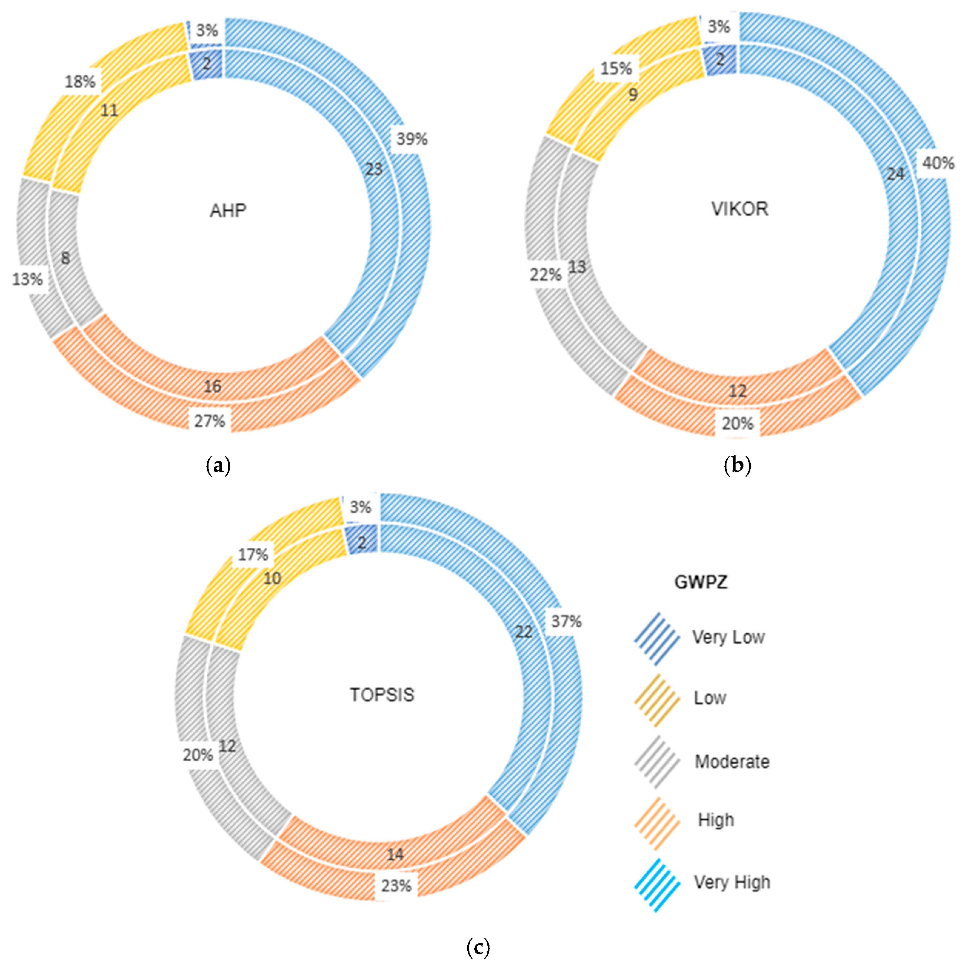
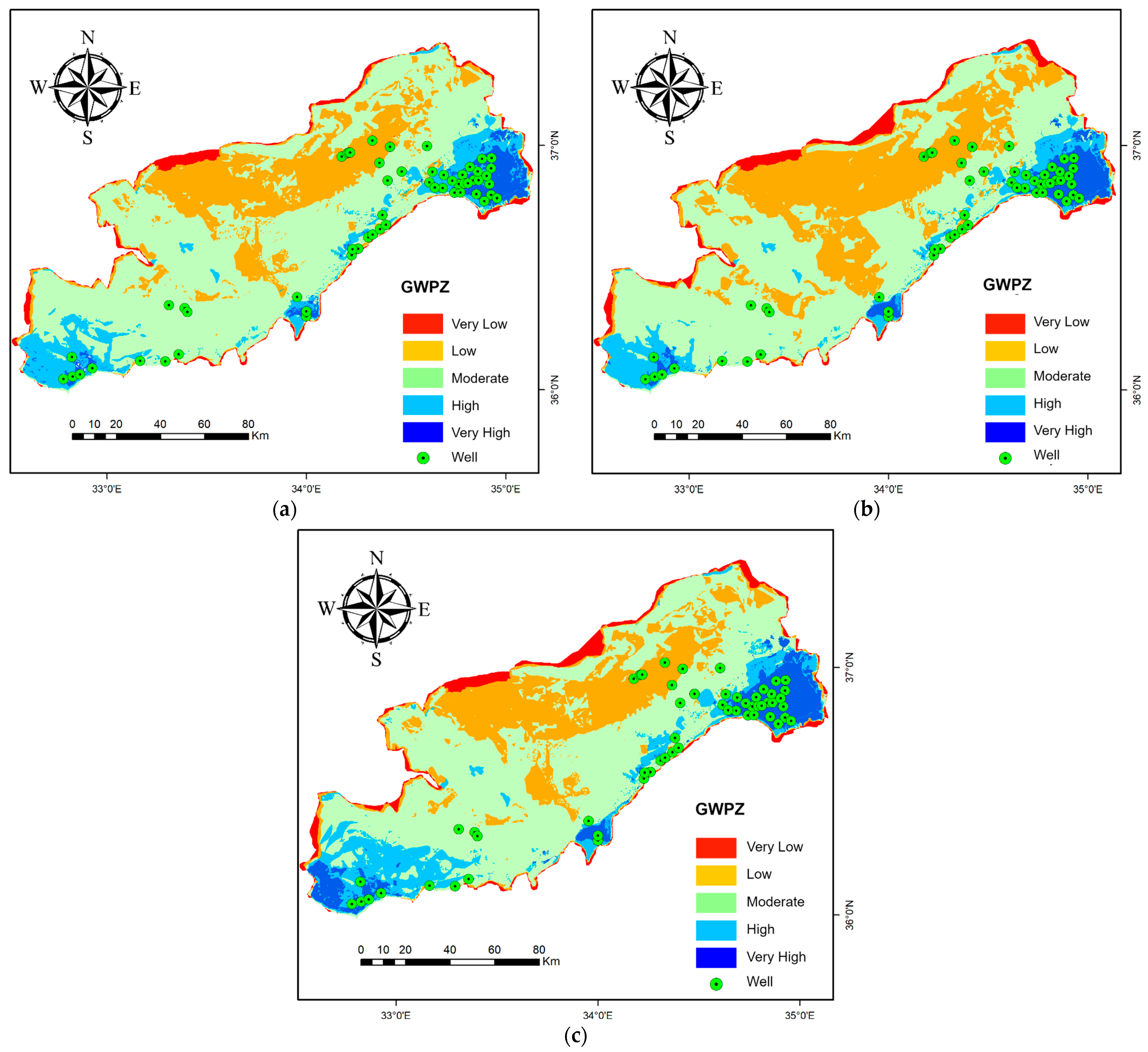
| Classes | AHP | VIKOR | TOPSIS | |||
|---|---|---|---|---|---|---|
| % Area | % Area | % Area | ||||
| Very Low | 345.23 | 2.18 | 443.38 | 2.80 | 487.38 | 3.07 |
| Low | 3373.18 | 21.28 | 4522.26 | 28.53 | 3313.61 | 20.90 |
| Moderate | 9618.81 | 60.68 | 8309.08 | 52.41 | 8173.84 | 51.56 |
| High | 1727.05 | 10.89 | 1636.26 | 10.32 | 2616.04 | 16.50 |
| Very High | 788.73 | 4.98 | 942.01 | 5.94 | 1262.14 | 7.96 |
| Total | 15,853 | 100 | ||||
Disclaimer/Publisher’s Note: The statements, opinions and data contained in all publications are solely those of the individual author(s) and contributor(s) and not of MDPI and/or the editor(s). MDPI and/or the editor(s) disclaim responsibility for any injury to people or property resulting from any ideas, methods, instructions or products referred to in the content. |
© 2024 by the authors. Licensee MDPI, Basel, Switzerland. This article is an open access article distributed under the terms and conditions of the Creative Commons Attribution (CC BY) license (https://creativecommons.org/licenses/by/4.0/).
Share and Cite
Çelik, M.Ö.; Kuşak, L.; Yakar, M. Assessment of Groundwater Potential Zones Utilizing Geographic Information System-Based Analytical Hierarchy Process, Vlse Kriterijumska Optimizacija Kompromisno Resenje, and Technique for Order Preference by Similarity to Ideal Solution Methods: A Case Study in Mersin, Türkiye. Sustainability 2024, 16, 2202. https://doi.org/10.3390/su16052202
Çelik MÖ, Kuşak L, Yakar M. Assessment of Groundwater Potential Zones Utilizing Geographic Information System-Based Analytical Hierarchy Process, Vlse Kriterijumska Optimizacija Kompromisno Resenje, and Technique for Order Preference by Similarity to Ideal Solution Methods: A Case Study in Mersin, Türkiye. Sustainability. 2024; 16(5):2202. https://doi.org/10.3390/su16052202
Chicago/Turabian StyleÇelik, Mehmet Özgür, Lütfiye Kuşak, and Murat Yakar. 2024. "Assessment of Groundwater Potential Zones Utilizing Geographic Information System-Based Analytical Hierarchy Process, Vlse Kriterijumska Optimizacija Kompromisno Resenje, and Technique for Order Preference by Similarity to Ideal Solution Methods: A Case Study in Mersin, Türkiye" Sustainability 16, no. 5: 2202. https://doi.org/10.3390/su16052202
APA StyleÇelik, M. Ö., Kuşak, L., & Yakar, M. (2024). Assessment of Groundwater Potential Zones Utilizing Geographic Information System-Based Analytical Hierarchy Process, Vlse Kriterijumska Optimizacija Kompromisno Resenje, and Technique for Order Preference by Similarity to Ideal Solution Methods: A Case Study in Mersin, Türkiye. Sustainability, 16(5), 2202. https://doi.org/10.3390/su16052202