Panel Data Analysis of Subjective Well-Being in European Countries in the Years 2013–2022

Dziechciarz, Marta

doi:10.3390/su16052124

Open AccessArticle

Panel Data Analysis of Subjective Well-Being in European Countries in the Years 2013–2022

by

Marta Dziechciarz

Department of Econometrics and Operations Research, Wroclaw University of Economics and Business, 53-345 Wroclaw, Poland

Sustainability 2024, 16(5), 2124; https://doi.org/10.3390/su16052124

Submission received: 26 December 2023 / Revised: 26 February 2024 / Accepted: 29 February 2024 / Published: 4 March 2024

(This article belongs to the Section Health, Well-Being and Sustainability)

Download

Browse Figures

Versions Notes

Abstract

:

The background of the study is the analysis of social expenditure efficiency in European countries over time. Terminological considerations leading from hedonism and eudaimonism to the concept of subjectively perceived well-being and the Easterlin paradox are necessary to understand the differences in changes in the level of well-being among countries and over time. The purpose of the study is to analyse citizens’ declarations on subjective well-being as an indicator of the efficiency of social policy. The methods used for statistical analysis are conventional and dynamic data envelopment analysis (DEA) techniques. The EU-SILC and OurWorldInData.org data analysed with DEA provided the main results. The study identified significant fluctuations in subjective well-being, with a clear long-term upward trend. Among the surveyed countries, there are those where progress is due to internal factors, while in the Mediterranean countries, external factors predominate. The level of the estimated DEA efficiency indicators (TC and EC) indicate the improvement in input efficiency in a substantive number of countries, e.g., Estonia and Cyprus, along with persistently low indicator values in some member states, Italy and Luxemburg. In conclusion, the author indicated areas in individual countries where attempts to improve social policy are needed to raise and maintain desirable levels of subjective well-being.

Keywords:

subjective well-being; household; DEA; panel DEA; dynamic DEA; Malmquist index; Cantril ladder; Easterlin paradox; spatiotemporal analysis; overall life satisfaction

Graphical Abstract

1. Introduction

The theoretical purpose of the considerations is to discuss the terminology related to the measurement and modelling of the subjective well-being of households.

The extent and efficiency of public spending on social programmes is a vital issue in exploring well-being. The cognitive goal of this article is to examine the relationship between the level of expenditure on selected aspects of the material and the perceived well-being of individuals and families (households’ subjective well-being level). The research design, applied methodology and analytical approach include the measurement, cross-sectional analysis, comparative description and modelling of the sustainability of households’ subjective well-being [1]. The selected statistical techniques serve as tools for describing, analysing and modelling the efficiency of socio-economic policy in the European Union countries in 2013–2022. Eurostat and the OurWorldInData.org platform provides data that is advantageous for this purpose. Statistical data on the European Union Statistics on Income and Living Conditions (EU-SILC) and Cantril ladder data available on the OurWorldInData.org platform served as data material used to achieve the cognitive goal of this article [2,3].

The problem of social programme effectiveness leads to this submission’s utilitarian goal, i.e., identifying countries with the most effective socio-economic policy. One may expect that in countries with the most effective socio-economic policy, the most significant increases in the indicators of the subjective well-being of households will occur [4,5,6,7,8].

The concept of well-being, which emerged in science in ancient times, has stood the test of time and now occupies a central place in social sciences. Interesting reflections on the evolution of human interest in the concept of well-being over the centuries, from the approach by tribal communities to the ancient Greeks, are contained in the works of [9,10,11].

The contemporary world literature provides a rich discussion on determining the meanings of terms related to measuring and modelling households’ subjective well-being. The starting point for the debate is the terminology regarding the quality of life and the material well-being of citizens and households. By extending the definitions of economic and technical circumstances formulated in this document to the general public, one can develop a good description of the quality of life [12,13].

Along with the substantial increase in many societies’ level of material well-being, the phenomenon of the sustainability of subjective well-being has become a hot topic in the social sciences, covering disciplines from psychology and economics to sociology, philosophy, literature, development studies, health, communication and media, education, public policy and many specialised fields. An additional impulse is the rapid development of positive psychology observed in recent decades, which has stimulated a broader interest in well-being [14,15,16,17,18].

The utilitarian goal of this submission consists of identifying the European Union member states with the most effective socio-economic policy. The hypothesis was that public expenditures were the most efficient in those countries where the most significant increases in the indications of the subjective well-being of households occurred [1,5,6].

The purpose of the work here is the consideration of terminology related to the measurement and analysis of the subjective well-being of households. The recent literature [19,20] illustrates the possibility of using data envelopment analysis (DEA) as an analytical tool for assessing well-being policy efficiency.

2. Theoretical Background

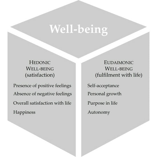
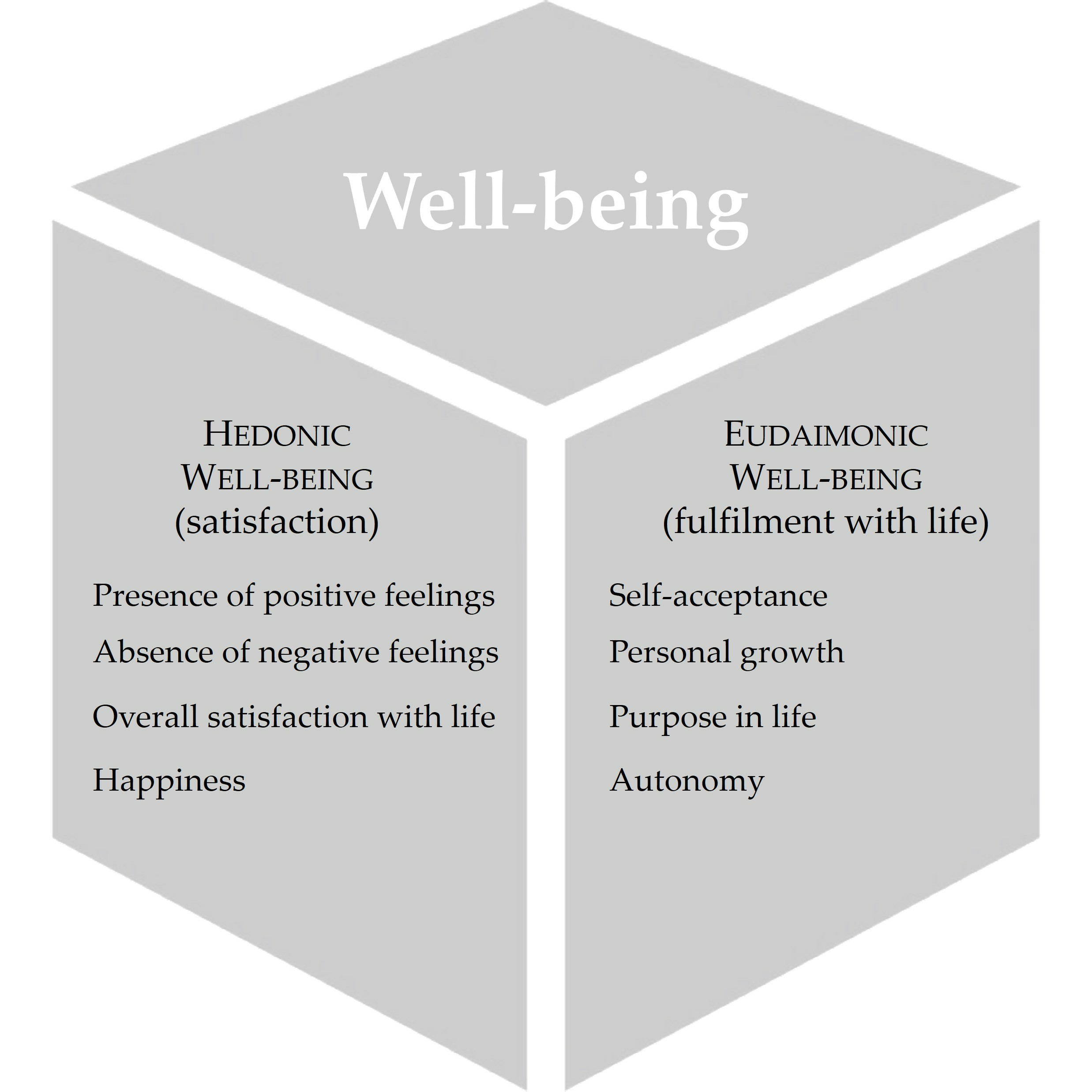
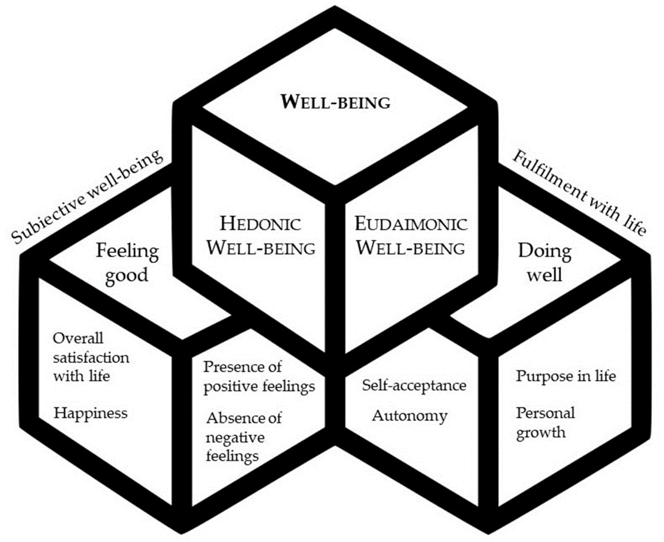
2.1. Subjective Well-Being

The general concept formulated by A. Sen [19] provided the theoretical basis for the considerations. Researchers use A. Sen’s concept of capability to construct tools for measuring the quality of life (QoL) [21,22,23,24,25,26]. A. Sen’s proposal has found wide acceptance as a tool of a specific normative theory used for the moral assessment of social structures, which are more cultural than developmental [27,28]. The context of the discussion is the terminology regarding the quality of life and the material well-being of citizens and households. The issue of precise definitions becomes even more complicated if the study covers the problem of the well-being of people with disabilities and families in which such people exist.

The starting point for the discussion of terminology is the assumption that measuring the quality of life and well-being, especially subjective well-being, does not describe identical phenomena. Indeed, they are not synonyms. The definition of quality of life includes an objective (measurable) assessment of people’s living conditions. The crucial aspect of the meaning of quality of life is the relationship between the individual circumstances of existence of an individual in the environment, understood as the socio-economic and technical conditions in which individual people and families function [13]. The human pursuit of well-being occupies space beyond simply seeking hedonic pleasure, feeling good and being satisfied. The second concept, called eudaimonia, aims at a stable social dimension (the idea of goodness) in which politics plays a central role. The subject of interest in this work is the level of subjective well-being (SWB) expressed by a household member, usually the head of the household [29,30,31,32,33,34,35,36]. Ed Diener is one of the leading representatives of hedonism research [37,38]. O. Medvedev and C. Landhuis are representatives of the eudaimonic tradition [39]. A. Frawley published a wide-ranging review of happiness concepts [40]. Figure 1 illustrates the concept of a well-being structure.

A fascinating study, unique on a global scale, was conducted by J. Czapiński in his research on an extensive sample of over twelve thousand households. It turned out that eudaemonists declared a higher quality of life—approximately 42% of them in Poland compared to 22% of hedonists [41].

2.2. The Easterlin Paradox

Based on the core meaning of subjective well-being, R. Easterlin formulated the theoretical approach valuable for international comparisons of subjective well-being. This contradiction is a paradox named after the scientist who first described it. In the literature, the proposal has a description of the Easterlin paradox. R. Easterlin noted that subjective well-being perception—happiness—varies along with income at a specific, fixed point in time. The phenomenon exists both between and within nations. Paradoxically, happiness does not always trend upward over time with increasing revenue. In other words, there is a contradiction between the point-of-time mechanism and time series findings. Since the 1970s, numerous publications have attempted to substantiate that paradox theoretically. Some researchers strongly dispute its existence, while others claim the inconsistency is solely an empirical generalisation. Extensive background and discussions may be found, among others, in [42,43,44,45,46,47,48].

The central thesis of the Easterlin Paradox is that subjectivism leads to relativism. As mentioned above, researchers define subjectivity in such a way that if someone says that she or he is happy, it definitely means that she or he is happy, regardless of the set of information supporting this assessment. Easterlin claims that the comparative aspects of subjective perception of well-being are equally significant to objective (measurable) values of quality of life elements. It comes to the observation that if I see that others are living much better than I am, I feel that what I am not doing is not good enough. The above phenomenon describes what probably happens in the wealthiest countries. While the majority of the population has their needs met, the display of wealth by the wealthy elite brings down those not so fortunate. In contrast, people in less affluent countries may feel happier because they have less to compare with (Figure 2) [48].

Differences in the subjective perception of well-being depend on several factors. In addition to material wealth, the possession of durable goods and financial resources, the philosophy of life is decisive. The differences in subjective well-being perception also depend on the type of household, township class and source of income [49].

The contemporary versions of the philosophy of life consider new developments in social life patterns. Identification of different causes of SWB may come from the growing popularity of circular economy and sharing consumption philosophies. Thus, the differences in ownership result not only from the socio-economic characteristics of a household. Some families cannot afford the durables they need, lacking financial resources and having no access to loans. Other family units do not possess individual durable goods simply because they feel no need for them, although they could finance the purchase from their funds or through a loan.

Figure 2 shows unexpected neighbourhoods of similar index values, an example of Easterlin’s Paradox. Some of these items are not obvious, considering the general, measurable level of citizens’ material wealth.

The non-parametric analytical technique, known in the literature as DEA, is a fairly common tool used in efficiency analysis on a microeconomic scale. The latest publications indicate the possibility of using the DEA technique to assess the effectiveness of socio-economic policies of countries, regions or management boards of individual parts of urban agglomerations. The discussed tool makes it possible to identify territorial units with the best and weaker results [20,50,51,52,53]. My work fills the gap in the literature by introducing the new cross-national and cross-temporal approach to assessing the social policy efficiency of national governments using the DEA.

3. Materials and Methods

The methodological approach undertakes important domains of well-being. Table 1 summarises the dimensions of well-being and their indicators. Indicators distinguishing four domains of subjective well-being have been indicated [1]. A domain that measures material conditions contains income aspects and job (productivity) indicators. The subsequent domain on the population and social conditions involves diverse aspects concerning social protection, e.g., benefits, sickness, healthcare, disability and old age and survivors. The successive domain of well-being that is concerned is quality of life [13]. Education, environment, health and safety indicators are significant factors influencing the well-being and quality of life of individuals. Indicators that measure the sustainability of well-being with an overall life experience are the average overall life satisfaction rating and self-reported life satisfaction, known as the Cantril life ladder score. The latter, developed by H. Cantril [54], is a ten-point measure widely used in opinion polls, e.g., by the OECD, Gallup and OurWorldInData, as the measure of subjective well-being [55,56,57,58].

Table 1 lists indicators that are potential proxies of well-being. The list is consistent with the literature, e.g., [56,57,58].

3.1. Data

The data used for analysis are from the annual research known as EU-SILC [2,3,59]. Thus, the dataset consists of compiled variables gathered for the available years, from 2013 to 2022, and for selected European countries. Specifically, the dataset encompasses selected indicators of quality of living dimensions and well-being of dimensions. Table 1 and Table 2 juxtapose variables (indicators) used as a proxy of well-being and quality of life (2013 to 2022).

Some variables describe personal or household (HH) well-being and self-reported life satisfaction. The estimated mean (and standard deviations—SD) for these variables for the population of 27 EU countries are presented in Table 2.

Table 3 shows the mean (and standard deviations) of variables describing material conditions and population and social conditions over ten years (for considered European countries). Worth noticing is that the long-term unemployment rate has decreased over the respective period. The tertiary educational attainment variable illustrates a positive change in people’s education. There is an increase in social protection benefits and median income.

The maps in Figure 3 show a ten-point scale rating of overall life satisfaction and self-reported life satisfaction (Cantril ladder score). In both cases, nevertheless, regardless of which variable is being taking into account, in 2022, the ratings of European countries such as Bulgaria and Romania are suffering the lowest levels of well-being assessment. Indicators used to measure the sustainability of well-being vary over time in particular countries. Even though the measures of subjective well-being fluctuate and change, a general increasing tendency exists. Bulgaria seems to be an outlier out of the twenty-seven EU countries in all years since 2013. Over ten years of chasing the level of, e.g., the Cantril life ladder, in 2022, Bulgaria stayed apart from the rest of the countries, but the distance is continually shrinking (Figure 4).

3.2. Methods of Data Analysis

The data envelopment analysis (DEA) approach is the methodical base in the present subjective well-being analysis and modelling study. DEA is a linear programming technique for measuring decision units’ technical, scale and allocative efficiency based on non-parametric frontier estimation. A. Charnes, W. Cooper and E. Rhodes published the proposal in 1978 [60]. F. Førsund and N. Sarafoglou comprehensively described DEA’s origins [61,62]. A discussion on recent developments and challenges is provided by A. Emrouznejad [63].

The DEA method is a non-parametric method used to measure and evaluate relative efficiency, i.e., to assess the performance of decision-making units (DMUs), such as territorial units, companies, organisations or economic sectors [64,65]. Researchers often use the discussed methodology because it captures and describes the interdependence between many variables on the input side (input data) and the effects side (result data). The literature points out that it is worth using the DEA research technique; it is the advisable alternative for parametric analysis. Numerous authors recommend the DEA methodology to assess the efficiency of socio-political policies [66,67,68,69,70,71]. The advantages of the data envelopment method include that it does not require specification or knowledge of variable weights. One can find numerous applications of DEA techniques in the literature. For example, ref. [72] described various applications for assessing the quality of healthcare work. Similar applications include banking, non-profit organisations, social welfare, military, health services, production organisations, educational institutions and police. The authors of publications [73,74,75,76] show examples of selected applications. A. Moradi-Motlagh and A. Emrouznejad provided an extensive, analytical overview of DEA developments in recent decades [77].

Based on the Malmquist idea, the dynamic DEA is the proper choice for analysing and comparing the results of DMUs (e.g., countries) in different periods. The DEA Malmquist productivity measure is an extension of the conventional DEA model devoted to the assessment of changes in productivity over time. Combining total productivity change into efficiency and productivity components provides a more detailed understanding and evaluation of the factors influencing overall productivity change. The Malmquist model focuses on analysing changes in efficiency and productivity over multiple periods. The Malmquist DEA approach has two key elements: efficiency change (EC) and total factor productivity change (TC). The efficiency change (EC) metric value illustrates the difference in DMU performance over time.

Furthermore, the efficiency change (EC) metric reflects the ability of the DMU to move towards a hypothetical boundary representing maximum efficiency. The efficiency change (EC) indicator describes the change in such a way that if the EC value is greater than unity, it indicates an improvement in efficiency over time, and values lower than unity indicate a decrease in efficiency. A situation where the EC value equals one means constant efficiency over time. The second indicator, the measure of total factor productivity (TC), assesses the overall change in the level of productivity resulting from technological progress and technical efficiency levels [78,79,80,81].

The website hosted by the University of Warwick in the UK [82] tracks and publishes the latest theoretical, methodological and application progress in the field of DEA.

The conventional, nondynamic DEA model does not consider that decisions regarding inputs result in effects extending beyond one period. Furthermore, it does not reflect possible medium- and long-term efficiency gains. The indicated aspects make a cross-sectional or even a panel data model insufficient to characterise the dynamic nature of the modelled process. In conclusion, it is worth noting that dynamic models are needed to describe the system’s behaviour mechanism over time. The concept of economic dynamic analysis means that researchers look at the change in the value of indicators over time. As a rule, time is a continuous variable. However, in economics, it is usually assumed that the level of a variable in one period is a function of the status of this variable in one or several previous time intervals (periods), i.e., one assumes the discrete nature of the time variable. In the described context, the Malmquist productivity index MI is one of the most frequently used tools [83]. The calculated values of MI indices are the basis for assessing the efficiency of the observed unit compared to the reference unit [84].

Table 1 indicates the complete list of variables taken into account. Table 4 presents a detailed list of variables selected from Table 1. The criteria for variable selection are their statistical properties and the requirements of DEA. The data envelopment analysis (DEA) methodology uses input and output data to measure and compare the efficiency of homogeneous decision-making units (DMUs—countries). They are input and output indicators. DEA input variables used to measure the efficiency in the production of well-being were as follows: net income, tertiary educational attainment and social protection, variables labelled I₁ to I₆ in Table 4. Output variables are the subjective well-being indicators, such as the ability to make ends meet (ratio of households making ends meet easily) and self-reported life satisfaction: Cantril ladder score (Table 4, outputs O₁ and O₂, respectively).

Section 4.1 presents the results of applying CRS and VRS versions of conventional DEA. Each was calculated for output-oriented specification. The data covered four analysed years: 2015, 2017, 2019 and 2021. The following Section 4.2 contains calculation results for the DEA panel model in the CRS and output-oriented versions. The panel covers data for the years 2013–2022.

4. Results

4.1. Conventional Data Envelopment Analysis (DEA)

In the present study, conventional DEA is used to analyse and illustrate subjective well-being for the four selected years. The first stage of the analysis is carried out separately for each of the four years: 2015, 2017, 2019 and 2021. Eight indicators illustrate the efficiency measure contributing to the sustainability of well-being perception (Table 1).

Table 5 juxtaposes ten-year mean values of inputs and outputs. The lowest ten-year mean value of assessment of self-reported life satisfaction is in Greece, Bulgaria, Croatia and Hungary. Similarly, the subjective evaluation of well-being is the ability to make ends meet: Greece and Bulgaria are among countries that report a very low ratio of households making ends meet easily. On the contrary, at the top of the list of countries appear the Netherlands, Germany and Belgium (according to the I₁ variable mean value), Finland, Denmark and the Netherlands (according to the mean value of the I₂ variable).

Notably, input variable values are low in Romania, Bulgaria, Hungary, Greece and Croatia. Considerably greater mean values of output variables are for Luxembourg, Denmark and the Netherlands. The wealthiest European countries undoubtedly use their capital (incur social protection expenditures) in their well-being production process.

Table 6 shows European countries’ relative efficiency scores in 2015, 2017, 2019 and 2021. One of the goals of the analysis was to distinguish between European countries that are efficient and inefficient in obtaining well-being. Thus, to estimate an indicator summarising well-being dimensions, output orientation VRS-DEA and output orientation CRS-DEA were performed in the analysis. The deaR package served for data processing [85]. The output orientation VRS-DEA analysis showed that eight countries in the four considered periods (years 2015, 2017, 2019 and 2021) had efficiency scores that were exactly one: the Netherlands, Bulgaria, Czechia, Denmark, Estonia, Poland, Romania, Finland, Italy and Germany. For five countries, the Netherlands, Estonia, Poland, Romania and Germany, the output-oriented CRS-DEA efficiency scores with values equal to one (for all years) can be observed.

In 2015, efficiency scores for output orientation VRS-DEA for ten European countries were one. That implies that the following countries operated on technical efficiency in 2015: the Netherlands, Bulgaria, Czechia, Denmark, Estonia, Poland, Romania, Finland, Italy, Germany and Malta. These countries employed inputs in optimal ways to produce well-being (the outputs). As shown in Table 6, CRS-DEA returned seven efficient countries. For VRS-DEA, either in 2015 or 2017, the least technically efficient countries were Greece and Portugal. Some high-GDP European countries, such as Luxemburg or France, had efficiency scores that placed them at the bottom of the ranking, with scores values greater than one indicating room for improvement.

Figure 5 shows the ranking of European countries based on the efficiency scores for all countries. The ranking was made by employing output-oriented VRS-DEA and output-oriented CRS-DEA. Both the VRS-DEA ranking and CRS-DEA show that the Netherlands, Czechia, Estonia, Poland, Romania, Bulgaria, Finland, Germany and Malta are countries that, in the majority of the considered years, are on the top efficiency rank (scores equal to 1).

It is possible that there is more than one country in the first, second or any of the following places. Surprisingly, according to this ranking, Luxemburg and France appeared among the least efficient countries. Among others that seem to be less efficient are Spain, Croatia, Cyprus, Hungary, Slovenia, Greece and Portugal. Most of the countries are relatively stable in the ranking. The exception is Malta, which notably fell in 2021 compared to the previous periods. Latvia, on the contrary, significantly jumped up over the last year.

Linking the DEA efficiency indicators is the tool for formulating practical policy measures. Policy-makers can get practical recommendations on how to enhance social policy. These recommendations need the distinction between internal and external and intercountry and intra-country factors that are affecting subjective well-being. Based on such an inference, differentiated policies are needed, taking into account mechanisms describing how factors interact and how they evolve over time. One of possibilities is the use of particularities of identified benchmark countries.

References (benchmark countries) are shown in Figure 6. Romania, the Netherlands and Germany are the most numerous benchmark countries for other countries in all years. Estonia and Czechia are benchmark countries in almost all periods. Some countries are benchmark countries only in one year, e.g., Italy, Finland and Belgium. It is evidently visible that benchmark countries are changing over the subsequent years. Hence, an additional analysis was performed, dynamic DEA along with the Malmquist productivity index, which explains, in more detail, the internal and external causes of efficiency changes over time.

4.2. The Dynamic Data Envelopment Analysis for Panel Data

The problem under investigation is the change in efficiency over time. The DEA-based Malmquist productivity index is an appropriate tool to capture changes in efficiency over time. The primary research instrument for the goal achievement in this submission is the dynamic version of DEA, i.e., the Malmquist productivity index (MPI) proposed by D. Caves et al. [83] based on S. Malmquist [86]. The Malmquist productivity index (MI) measures changes in DMI over time—here, in European countries.

The dynamic DEA for the panel data was the next research stage. The same indicators as for the conventional DEA served to model the dynamic efficiency in producing well-being. Table 4 indicates the list of variables under investigation. Again, the DEA output variables were the subjective well-being indicators, such as the ability to make ends meet (ratio of households making ends meet easily) and self-reported life satisfaction: Cantril ladder score (Table 4, outputs O₁ and O₂, respectively). Input variables used to measure the efficiency in the production of well-being over time were net income, tertiary educational attainment and social protection, variables labelled I₁ to I₆ in Table 4. Table 7 contains values of output orientation DEA efficiencies (CRS) for 2013 to 2022.

As seen in Table 7, four countries had all efficiencies between two periods equal to one. Germany, Estonia, the Netherlands and Romania experienced constant efficiency. For these countries, efficiency (productivity) did not change from 2013 to 2022. Most of the time, numerous countries did not maintain the maximum efficiency between the two periods. Ireland, Luxemburg, Greece and France faced the lowest efficiencies in the period under research. There is room for improvement. The efficiency scores increased slightly from period to period, e.g., in Greece and France. In some countries, there was a decrease in the efficiency scores, even though there had also been efficiencies between two periods equal to one. For example, in Italy, there was a decreasing tendency in the period examined.

Figure 7 shows the Malmquist index output orientation DEA in the subsequent ten years. The Malmquist index indicates an improvement in productivity over time. The constant returns to scale (CRS) index is a tool for investigating whether efficiency improvements originate in technological or productivity changes.

Some countries do not have any significant changes in productivity over time since the MI value is close to one. For instance, countries with a constant productivity level between the two periods (and close to one) are Denmark and Germany. This means that countries with an MI value higher than one, such as Cyprus, achieved productivity growth, in particular in the periods after 2016. Compared to Latvia and Malta (in 2015), as well as Spain and France (in 2020), Poland has been relatively stable over time.

Table 8 juxtaposes the efficiency change (EC) and the technological change (TC), which decompose the Malmquist Index (MI). The Malmquist Index does not justify specific factors contributing to productivity changes. Accordingly, the efficiency change (EC) and the technological change (TC) from 2013 to 2022 may give a more comprehensive understanding of the source and character of improvements.

A thought-provoking country to analyse is Cyprus. There are evidently visible changes over time. An improvement in productivity over time in Cyprus, after 2016, shows that the efficiency change (EC) is 0.79 and the technological change (TC) is precisely equal to one. This may suggest that the efficiency change strongly depends on external factors, in this case, unfavourable ones, including the Russian annexation of Crimea and the related banking crisis and also COVID-19. The indicated factors are probably the cause of EC index values that are less than unity. Values of the TC indicator greater than or equal to unity indicate the efficient and effective management of social policy expenditures (input variables).

5. Discussion and Limitations

The contribution of this work to the development of the theoretical and empirical state of knowledge lies in three aspects. The first aspect is an attempt to summarise the terminological interpretation of common concepts that constitute subjective well-being. The text contains philosophical discussions summarising the consequences resulting from terminological conditions for measuring and determining the typology of the subjective well-being of households.

The second area in which the article contributes is the cognitive aspect of deepening knowledge about the relationship between the country’s expenditure on selected material aspects and the perceived well-being of individuals and families. In extensive experimental research, the dynamic DEA served as a tool to describe and analyse the effectiveness of socio-economic policy in European Union countries in 2013–2022. The data used to achieve the cognitive goal of the article were European Union statistical data on income and living conditions (EU-SILC) and Cantril ladder data available on the OurWorldInData.org platform. Eurostat and the OurWorldInData.org platform provide data for this purpose. The analytical approach included measurement, cross-sectional and cross-national analyses. The base for the recommendations for decision-making and a comparative description of the sustainability of the subjective well-being of households in EU countries were the results of in-depth studies on sources of the level and dynamics of SWB.

The approach used, in terms of the types of data used and the sources of information, combined with a dynamic version of DEA using extensive cross-sectional data covering ten years and twenty-seven countries, is a unique, previously unused research approach. The concept that all EU countries, with data covering the last ten years, are simultaneously analysed is unique and has never been conducted before. The approach gives a solid base for describing the efficiency over the period and across the countries. The analysed period includes important events disrupting the operation of inputs, particularly the Russian invasion of Ukraine in 2014 and the challenging period of the COVID-19 pandemic.

The contribution to the utilitarian knowledge contained in this submission is to identify the European Union member states with the most effective socio-economic policies and the countries with the most effective socio-economic policies and to consider the factors influencing the effectiveness and the resulting policy regarding social spending. There appears to be no published work that studies countries with the most effective socio-economic policies that will see the most significant increases in indicators of the subjective well-being of households. Additionally, the contribution to the utilitarian knowledge of this application consists of its attempt to develop decision-making recommendations for specific types of countries.

The gathered knowledge from the study’s results may help to conduct social policy in individual countries and the European Union. Political declarations of respective governments contain goals for building and strengthening economic and social cohesion. Strategic goals regarding social security include National and EU documents [87,88,89].

In this context, A. Moro-Egido et al. discuss the role of economic and social resources and justify improving the sustainability of well-being over time [90]. The issue enjoys broad interest in the literature [91,92,93,94].

One should remember that the collected data cover periods of two events that significantly influenced the situation in Europe. These events are Russia’s aggression against Ukraine in 2014, which resulted in severe disruptions in the financial and banking markets. It mainly affected Cyprus. The second event was the COVID-19 epidemic, which affected all countries, but most severely those whose situation depends on tourism. Both events are impressive and strongly reflect the respondents’ feelings, described in the modelled variables: overall life satisfaction and the Cantril ladder score.

Limitations. The limitations of the inference from the results of the current study are twofold: the data and their quality and the analytical tool—dynamic DEA and its applicability. Understanding the impact of public spending on well-being requires the availability of data collected through rigorous measurements that consider variations in local socio-economic and political factors. The primary source of limitations to the validity of the conclusions from the study is the quality of available statistical data. Measuring efficiency resulting from the phenomenon’s complexity, including expenditure on social purposes (education, health, culture, sports), environmental protection and public administration, determines the data quality. There are more problems when attempting international and cross-sectional analyses. Although there has been significant progress in developing measurement techniques, the availability of appropriate data remains a challenge. However, Eurostat has made significant progress in unifying how it defines and measures phenomena in the European Union’s member states. A similar observation applies, although to a lesser extent, to other international organisations, the OECD, the UN, the World Bank and global research communities, including OurWorldinData.

A significant limitation is the adopted theoretical basis underlying the formulated inference rules. In the empirical literature, various data operationalisation paradigms exist in measuring the effectiveness of public spending. However, the usual assumption holds that the effects of public expenditures are multilateral and manifest themselves in various sectors of society.

The second important source limiting the validity of the conclusions resulting from the study is the selected research technique. The study used data envelopment analysis (DEA) to assess the effectiveness of public spending. The DEA technique empirically measures the efficiency of the production of decision-making units (DMUs), in which it compares possible combinations of inputs (inputs) and outputs (effects), i.e., handling multiple inputs and outputs. This technique has gained popularity in research because it does not require any assumptions, allows for comparing multidimensional input and output data and is relatively simple computationally. The argument for using DEA to measure the effectiveness of government spending on well-being covers the main features of this research technique, including its multidimensional assessment and non-parametric approach, which allows for the inclusion of multiple inputs and outputs, providing a comprehensive and multidimensional assessment of social policy governance.

In the present study, the feature limiting the quality of inferences may be the failure to meet an essential assumption of DEA, which requires the homogeneity of decision-making units. In other words, all entities should operate under similar conditions. In the context of the presented study, there are significant differences in the nature of the studied objects (countries), their location in European regions, population diversity and historical and cultural differences, which DEA may not fully consider. The unified data collection method, which involves recording respondents’ declarations, supported the admissibility of the DEA technique.

In summary, understanding the efficiency of public spending is essential to optimising resource allocation and ultimately improving a nation’s subjective perception of well-being. In the last quarter of the 21st century, improving the efficiency and effectiveness of public spending is crucial, mainly due to the increased pressure on the stability of public finances. Continued demand for infrastructure investment and defence spending competes with the essential social needs of voters. The mentioned phenomenon is caused, among others, by long-term demographic trends and increased egalitarian self-awareness of societies. Influential social groups expect higher spending on continuing education, pensions, long-term care, etc. Recent scientific publications reflect the importance of the issue under discussion. Several publications deal with the conceptual problems of practical conditions of public sector efficiency [95,96,97]. The international approach to public spending efficiency concentrates on large organisations: the OECD [98] and the UN [99]. The research on EU countries represented by works by L. Baciu and A. Botezat [100] and the EU official document [101] concentrates on descriptive characteristics of selected problems without cross-sectional and inter-temporal aspects.

6. Conclusions

The analysis’s main conclusion is that the sustainable level of well-being in individual European Union countries is loosely related to objective indicators of material well-being. This is a typical situation under the Easterlin paradox. For example, the indications of the subjective well-being of citizens in Germany and Luxembourg are relatively low, lower than in countries such as Romania, Poland or Estonia. Another conclusion is the indication of large, and in the case of some countries, considerable fluctuations in declarations of the level of subjective well-being. The most significant differences in statements (year to year) were observed, among others, in Cyprus and Greece.

Recommendations, from the political point of view, may come from the significant fluctuations in the SWB assessment declarations indicating that citizens observe an increase in social inequalities. Therefore, governments should intensify efforts to fill the gaps between social groups. In the first place, this applies to Greece and Cyprus.

As suggested by the Easterlin paradox, the indications of the subjective well-being of citizens in fast-growing economies, including Central and Eastern European countries, manifest higher SWB perceptions than established, traditionally more prosperous societies. The underlying causal factors are unknown, and the results should be interpreted with caution. However, it may be speculated that inhabitants in Central and Eastern European are closer to hedonic philosophy, where citizens appreciate their overall improvement in their material situation. This may lead to a decrease in negative feelings.

Based on the conventional DEA analysis, it is evident that the level of input efficiency is subject to significant fluctuations in some countries. The utmost changes occur in countries with a lower level of material well-being. Fewer differences occur in wealthy countries, e.g., Germany and the Netherlands. Despite significant changes in the efficiency index in individual countries, a clear upward trend exists in the analysed years 2013–2022. Conventional DEA indicates that in most of the considered years, in both VRS- or CRS-based ranking, the Netherlands, Finland, Germany and Malta are countries that top the efficiency rank.

On the other hand, Czechia, Estonia, Poland, Romania and Bulgaria are those that are catching up. On average, the efficiency of inputs in less wealthy countries is higher than in rich countries. The conclusion is due to the observed phenomenon that the increase in well-being perception requires relatively less additional input than in wealthy countries, where it is much harder to achieve the growth of the declaration level.

For an in-depth analysis, the dynamic, output-oriented version of DEA was used. The results obtained with the Malmquist DEA include the efficiency change (EC) and technological change (TC) indexes. The technical efficiency index (or the so-called technological change index) equal to or higher than one, proving the highest value, indicates an improvement in efficiency due to progress in allocating funds for social policy purposes. In other words, this means an increasingly efficient way of using inputs and an increasingly better management of input usage exist. The technical efficiency index equal to or higher than one appeared in seven of the eleven examined years in Estonia and Cyprus. In 2013–2022, an index equal to or higher than one happened six times in Poland and Slovakia. At the same time, there were countries where the technical efficiency index equal to or higher than one occurred only occasionally, e.g., Italy and Luxembourg. This probably means that with high input efficiency, improving the manner of spending inputs is difficult. The recommendation for less efficient governments is twofold. First, untapped opportunities could be applied to current social policy to achieve additional, cost-free improvements in the perception of SWB. Secondly, knowledge and skills in improving spending efficiency should come from comparative analyses, leading to the identification of benchmarks. It is essential to understand how countries manage social spending more effectively.

It is worth mentioning that, in 2020, the TC index in all countries was less than one. It seems that this occurred because the authorities in all countries were still searching for an effective way to respond to the profound crisis of the sustainability of well-being caused by the COVID-19 pandemic.

The results of this submission could be the basis for designing an effective socio-economic policy at the national level. In the international context, the obtained results confirm the observation formulated in [102,103]. Some fast-growing economies, including Poland, produce higher subjective material well-being perceptions than established, traditionally more prosperous societies [104,105].

Funding

This research received no external funding.

Institutional Review Board Statement

Not applicable.

Informed Consent Statement

Not applicable.

Data Availability Statement

The data presented in this study are available on request from the corresponding author.

Conflicts of Interest

The author declares no conflicts of interest.

References

Jarden, A.; Roache, A. What is Well-being? Int. J. Environ. Res. Public Health 2023, 20, 5006. [Google Scholar] [CrossRef]
EU-SILC. European Union Statistics on Income and Living Conditions. 2023. Available online: https://ec.europa.eu/eurostat/web/income-and-living-conditions (accessed on 15 September 2023).
Happiness-Cantril-Ladder. Available online: https://ourworldindata.org/grapher/happiness-cantril-ladder (accessed on 15 September 2023).
Antonelli, M.; De Bonis, V. How Efficient is Welfare for Families? Evidence from European Countries. Appl. Econ. Lett. 2021, 28, 383–386. [Google Scholar] [CrossRef]
Frenda, A.; Sepe, E.; Scippacercola, S. Efficiency Analysis of Social Protection Expenditure in the Italian Regions. Socio-Econ. Plan. Sci. 2021, 73, 100965. [Google Scholar] [CrossRef]
Hu, Y.; Wu, Y.; Zhou, W.; Li, T.; Li, L. A Three-Stage DEA-Based Efficiency Evaluation of Social Security Expenditure in China. PLoS ONE 2020, 15, e0226046. [Google Scholar] [CrossRef]
Antonelli, M.; De Bonis, V. The Efficiency of Social Public Expenditure in European Countries: A Two-Stage Analysis. Appl. Econ. 2019, 51, 47–60. [Google Scholar] [CrossRef]
Huang, L.; Kern, M.; Oades, L. Chinese International Students’ Conceptualisations of Well-being. A Prototype Analysis. Front. Psychol. 2022, 13, 939576. [Google Scholar] [CrossRef] [PubMed]
Yadeun-Antuñano, M. Indigenous Perspectives of Well-being. Living a Good Life. In Good Health and Well-Being. Encyclopedia of the UN Sustainable Development Goals; Fernandez, R.M., Leal Filho, W., Wall, T., Azul, A., Brandli, L., Özuyar, P., Eds.; Springer: Cham, Switzerland, 2020. [Google Scholar] [CrossRef]
Alexandrova, A. Philosophy for the Science of Well-Being, Online ed.; Oxford Academic: Oxford, UK, 2017. [Google Scholar] [CrossRef]
Angner, E. The Evolution of Eupathics. The Historical Roots of Subjective Measures of Well-being. Int. J. Well-Being 2011, 1, 4–41. [Google Scholar] [CrossRef]
Convention on the Rights of Persons with Disabilities (CRPD). UN, 2006. Available online: https://social.desa.un.org/issues/disability/crpd/convention-on-the-rights-of-persons-with-disabilities-crpd (accessed on 15 December 2023).
Maggino, F.; Zumbo, B. Measuring the Quality of Life and the Construction of Social Indicators. In Handbook of Social Indicators and Quality of Life Research; Land, K., Michalos, A., Sirgy, M., Eds.; Springer: New York, NY, USA, 2012; pp. 201–238. [Google Scholar] [CrossRef]
Wang, C.; Wang, X.; Wang, Y.; Zhan, J.; Chu, X.; Teng, Y.; Liu, W.; Wang, H. Spatio-temporal Analysis of Human Well-being and its Coupling Relationship with Ecosystem Services in Shandong Province, China. J. Geogr. Sci. 2023, 33, 392–412. [Google Scholar] [CrossRef]
Kim, H.; Doiron, K.; Warren, M.; Donaldson, S. The International Landscape of Positive Psychology Research. A Systematic Review. Int. J. Well-Being 2018, 8, 50–70. [Google Scholar] [CrossRef]
Slade, M.; Oades, L.; Jarden, A. (Eds.) Well-Being, Recovery and Mental Health; Cambridge University Press: Cambridge, UK, 2017. [Google Scholar] [CrossRef]
Eger, R.; Maridal, J. A Statistical Meta-analysis of the Well-being Literature. Int. J. Well-Being 2015, 5, 45–74. [Google Scholar] [CrossRef]
Rusk, R.; Waters, L. A Psycho-social System Approach to Well-being. Empirically Deriving the Five Domains of Positive Functioning. J. Posit. Psychol. 2015, 10, 141–152. [Google Scholar] [CrossRef]
Sarracino, F.; O’Connor, K. A Measure of Well-Being Efficiency Based on the World Happiness Report; GLO Discussion Paper, No. 1061; Global Labor Organization: Essen, Germany, 2022. [Google Scholar]
Lafuente, E.; Szerb, L.; Acs, Z. Country Level Efficiency and National Systems of Entrepreneurship. A Data Envelopment Analysis Approach. J. Technol. Transf. 2016, 41, 1260–1283. [Google Scholar] [CrossRef]
Sen, A. Human Rights and Capabilities. J. Hum. Dev. 2005, 6, 2. [Google Scholar] [CrossRef]
Sen, A. The Idea of Justice; Penguin: London, UK, 2010. [Google Scholar]
Garcés, P. Humanizing Development. Taking Stock of Amartya Sen’s Capability Approach. Probl. Desarro. Rev. Latinoam. Econ. 2020, 51, 69586. [Google Scholar] [CrossRef]
Garcés, P. The Reasoning Agent. Agency in the Capability Approach and some Implications for Development Research and Practice. Iberoam. J. Dev. Stud. 2019, 9, 268–292. [Google Scholar] [CrossRef]
Garcés, P. Of Ends and Means. Development Policy Assessment with Human Development and Multiple Causality. Desarro. Soc. 2019, 83, 385–412. [Google Scholar] [CrossRef]
Sen, A. Choice, Welfare and Measurement; Blackwell: Oxford, UK, 1982. [Google Scholar]
Nussbaum, M.; Glover, J. Women, Culture, and Development. A Study of Human Capabilities; Oxford University Press: Oxford, UK, 1995. [Google Scholar] [CrossRef]
Nussbaum, M.; Sen, A. (Eds.) The Quality of Life; Oxford University Press: Oxford, UK, 1993. [Google Scholar]
Schaffner, K. Hedonic versus Eudaimonic Well-Being. How to Reach Happiness. 2023. Available online: https://positivepsychology.com/hedonic-vs-eudaimonic-wellbeing/ (accessed on 15 December 2023).
Quality of Life Indicators. Overall Experience of Life. 2023. Available online: https://ec.europa.eu/eurostat/statistics-explained/index.php?title=Quality_of_life_indicators_-_overall_experience_of_life (accessed on 25 December 2023).
Wei, Z. Refining the Concept of Eudaimonia. Commun. Humanit. Res. 2023, 4, 432–437. [Google Scholar] [CrossRef]
Cherry, K. What Is Self-Determination Theory? How Self-Determination Influences Motivation. 2022. Available online: https://www.verywellmind.com/what-is-self-determination-theory-2795387 (accessed on 15 December 2023).
Hedonism or Eudaimonism. Econation, 2022. Available online: http://econation.one/blog/hedonism-or-eudaimonism/ (accessed on 15 December 2023).
Hooker, S.; Masters, K.; Ranby, K. Integrating meaning in life and self-determination theory to predict physical activity adoption in previously inactive exercise initiates enrolled in a randomised trial. Psychol. Sport Exerc. 2020, 49, 101704. [Google Scholar] [CrossRef]
Heintzelman, S. Eudaimonia in the Contemporary Science of Subjective Well-being. Psychological Well-being, Self-determination, and Meaning in Life. In Handbook of Well-Being; Diener, E., Oishi, S., Tay, L., Eds.; DEF Publishers: Salt Lake City, CT, USA, 2018. [Google Scholar]
Diener, E. Subjective Well-being. Psychol. Bull. 1984, 95, 542–575. [Google Scholar] [CrossRef]
Diener, E.; Biswas-Diener, R. Happiness: Unlocking the Mysteries of Psychological Wealth; Blackwell Publishing: Malden, MA, USA, 2008. [Google Scholar]
Veenhoven, R. Subjective Measures of Well-being. In Human Well-Being: Studies in Development Economics and Policy; McGillivray, M., Ed.; Palgrave Macmillan: London, UK, 2007. [Google Scholar] [CrossRef]
Medvedev, O.; Landhuis, C. Exploring Constructs of Well-being, Happiness and Quality of Life. PeerJ 2018, 6, e4903. [Google Scholar] [CrossRef]
Frawley, A. Happiness Research. A Review of Critiques. Sociol. Compass 2015, 9, 62–77. [Google Scholar] [CrossRef]
Czapiński, J. Teorie szczęścia w świetle danych z Diagnozy Społecznej. In Diagnoza Społeczna. Warunki i Jakość Życia Polaków; Czapiński, J., Panek, T., Eds.; Rada Monitoringu Społecznego: Warszawa, Poland, 2009; pp. 163–175. [Google Scholar] [CrossRef]
Easterlin, R.; O’Connor, K. The Easterlin Paradox. In IZA Discussion Paper; Springer: Cham, Switzerland, 2020; p. 13923. [Google Scholar]
Easterlin, R. Happiness and Economic Growth. The Evidence. In IZA Discussion Paper; Springer: Amsterdam, The Netherlands, 2013; Volume 7187, pp. 1–32. [Google Scholar]
Easterlin, R. Does Economic Growth Improve the Human Lot? In Essays in Honour of Moses Abramovitz; David, P., Reder, M., Eds.; Academic Press: New York, NY, USA, 1974; pp. 89–125. [Google Scholar]
Li, L.; Shi, L. Economic Growth and Subjective Well-being. Analysing the Formative Mechanism of Easterlin Paradox. J. Chin. Sociol. 2019, 6, 1. [Google Scholar] [CrossRef]
Edsel, B. Income Growth and Happiness. Reassessment of the Easterlin Paradox, MPRA. 2014, pp. 1–33. Available online: https://mpra.ub.uni-muenchen.de/53360/1/MPRA_paper_53360.pdf (accessed on 15 December 2023).
Coppola, G. The Easterlin Paradox. An Interpretation. J. Happiness Econ. Interpers. Relat. 2013, 1–13. [Google Scholar] [CrossRef]
Clark, A.; Frijters, P.; Shields, M. Relative Income, Happiness, and Utility. An Explanation for the Easterlin Paradox and Other Puzzles. J. Econ. Lit. 2008, 46, 95–144. [Google Scholar] [CrossRef]
Bimonte, S.; Faralla, V. Does Residents’ Perceived Life Satisfaction Vary with Tourist Season? A Two-step Survey in a Mediterranean Destination. Tour. Manag. 2016, 55, 199–208. [Google Scholar] [CrossRef]
Debnath, R.; Shankar, R. Does Good Governance Enhance Happiness. A Cross Nation Study. Soc. Indic. Res. 2014, 116, 235–253. [Google Scholar] [CrossRef]
DiMaria, C.; Peroni, C.; Sarracino, F. Happiness matters: Productivity gains from subjective well-being. J. Happiness Stud. 2020, 21, 139–160. [Google Scholar] [CrossRef]
Emrouznejad, A.; Yang, G. A Survey and Analysis of the First 40 Years of Scholarly Literature in DEA: 1978–2016. Recent Developments on the Use of DEA in the Public Sector. Socio-Econ. Plan. Sci. 2018, 61, 4–8. [Google Scholar] [CrossRef]
Liu, J.; Lu, L.; Lu, W.; Lin, B. A survey of DEA applications. Omega 2013, 41, 893–902. [Google Scholar] [CrossRef]
Cantril, H. The Pattern of Human Concerns; Rutgers University Press: New Brunswick, NJ, USA, 1965. [Google Scholar]
Ortiz-Ospina, E.; Roser, M. Happiness and Life Satisfaction. OurWorldinData. Available online: https://ourworldindata.org/happiness-and-life-satisfaction (accessed on 15 September 2023).
OECD. How’s Life? Measuring Well-Being; OECD Publishing: Paris, France, 2020.
Helliwell, J.F.; Huang, H.; Norton, M.; Goff, L.; Wang, S. World Happiness Report 2023; Sustainable Development Solutions Network: New York, NY, USA, 2023; Available online: https://worldhappiness.report/ed/2023/ (accessed on 15 September 2023).
Measuring Household Wealth through Surveys. In OECD Guidelines for Micro Statistics on Household Wealth; OECD Publishing: Paris, France, 2013.
World Happiness Report processed by Our World in Data. Available online: https://worldhappiness.report/ (accessed on 15 September 2023).
Charnes, A.; Cooper, W.; Rhodes, E. Measuring the Efficiency of Decision Making Units. Eur. J. Oper. Res. 1978, 2, 429–444. [Google Scholar] [CrossRef]
Førsund, F. Dynamic Efficiency Measurement. In Benchmarking for Performance Evaluation; Ray, S., Kumbhakar, S., Dua, P., Eds.; Springer: New Delhi, India, 2015. [Google Scholar] [CrossRef]
Førsund, F.; Sarafoglou, N. On the Origins of Data Envelopment Analysis. J. Product. Anal. 2002, 17, 23–40. [Google Scholar] [CrossRef]
Emrouznejad, A.; Yang, G.L.; Khoveyni, M.; Michali, M. Data Envelopment Analysis. Recent Developments and Challenges. In The Palgrave Handbook of Operations Research; Salhi, S., Boylan, J., Eds.; Palgrave Macmillan: Cham, Switzerland, 2022. [Google Scholar] [CrossRef]
Hosseinzadeh Lotfi, F.; Allahviranloo, T.; Shafiee, M.; Saleh, H. (Eds.) Uncertainty in Data Envelopment Analysis; Elsevier: New York, NY, USA, 2023. [Google Scholar] [CrossRef]
Karliński, W. Data Envelopment Analysis in Performance Auditing. Kontrola Państwowa 2022, 46, 560–580. [Google Scholar] [CrossRef]
Jung, S.; Son, J.; Kim, C.; Chung, K. Efficiency Measurement Using Data Envelopment Analysis (DEA) in Public Healthcare. Research Trends from 2017 to 2022. Processes 2023, 11, 811. [Google Scholar] [CrossRef]
Smętek, K.; Zawadzka, D.; Strzelecka, A. Examples of the use of Data Envelopment Analysis (DEA) to Assess the Financial Effectiveness of Insurance Companies. Procedia Comput. Sci. 2022, 207, 3924–3930. [Google Scholar] [CrossRef]
Ghobadi, S.; Jahanshahloo, G.R.; Lotfi, F.H.; Rostamy-Malkhalifeh, M. Efficiency Measure under Inter-temporal Dependence. Int. J. Inf. Technol. Decis. Mak. 2018, 17, 657–675. [Google Scholar] [CrossRef]
Wolszczak-Derlacz, J. An Evaluation and Explanation of (in)efficiency in Higher Education Institutions in Europe and the US with the Application of Two-stage Semi-parametric DEA. Res. Policy 2017, 46, 1595–1605. [Google Scholar] [CrossRef]
Castelli, L.; Pesenti, R. Network, Shared Flow and Multi-level DEA Models: A Critical Review. In Data Envelopment Analysis; International Series in Operations Research & Management Science; Springer Science+Business Media: New York, NY, USA, 2014; Volume 208, pp. 329–376. [Google Scholar] [CrossRef]
Banker, R.; Emrouznejad, A.; Lopes, A.L.M.; de Almeida, M.R. Data Envelopment Analysis. Theory and Applications; University Rio Grande do Norte: Rio Grande, OH, USA, 2012; ISBN 978 185449 437 5. [Google Scholar]
Zubir, M.Z.; Noor, A.A.; Rizal, A.M.; Harith, A.A.; Abas, M.I.; Zakaria, Z.; Bakar, A.F.A. Approach in Inputs & Outputs Selection of Data Envelopment Analysis (DEA) Efficiency Measurement in Hospital. A Systematic Review. medRxiv 2023. [Google Scholar] [CrossRef]
Mohamadi, E.; Kiani, M.M.; Olyaeemanesh, A.; Takian, A.; Majdzadeh, R.; Hosseinzadeh Lotfi, F.; Sharafi, H.; Sajadi, H.S.; Goodarzi, Z.; Noori Hekmat, S. Two-step Estimation of the Impact of Contextual Variables on Technical Efficiency of Hospitals. The Case Study of Public Hospitals in Iran. Front. Public Health 2022, 9, 1839. [Google Scholar] [CrossRef]
Panwar, A.; Olfati, M.; Pant, M.; Snasel, V. A Review on the 40 Years of Existence of Data Envelopment Analysis Models. Historic Development and Current Trends. Arch. Comput. Methods Eng. 2022, 29, 5397–5426. [Google Scholar] [CrossRef]
Brzezicki, Ł. The Efficiency of Public and Private Higher Education Institutions in Poland. Gospod. Nar. Pol. J. Econ. 2020, 304, 33–51. [Google Scholar] [CrossRef]
Paradi, J.; Zhu, H. A Survey on Bank Branch Efficiency and Performance Research with Data Envelopment Analysis. Omega 2013, 41, 61–79. [Google Scholar] [CrossRef]
Moradi-Motlagh, A.; Emrouznejad, A. The Origins and Development of Statistical Approaches in Non-parametric Frontier Models. A Survey of the First Two Decades of Scholarly Literature (1998–2020). Ann. Oper. Res. 2022, 318, 713–741. [Google Scholar] [CrossRef]
Guo, D.; Cai, Z. An Integrated Slacks-Based Measure of Super-Efficiency with Input Saving and Output Surplus Scaling Factors and its Application in Paper Chemical Mills. J. Chem. 2020, 2020, 6161343. [Google Scholar] [CrossRef]
Fallah-Fini, S.; Triantis, K.; Johnson, A. Reviewing the Literature on Non-parametric Dynamic Efficiency Measurement. State-of-the-art. J. Product. Anal. 2014, 41, 51–67. [Google Scholar] [CrossRef]
Ray, S. Data Envelopment Analysis: A Non-parametric Method of Production Analysis. In Handbook of Production Economics; Ray, S., Chambers, R., Kumbhakar, S., Eds.; Springer: Singapore, 2022. [Google Scholar] [CrossRef]
Sengupta, J. Dynamics of Data Envelopment Analysis. Theory of Systems Efficiency; Springer: Dordrecht, The Netherlands, 1995. [Google Scholar] [CrossRef]
State-of-the-Art Information on Data Envelopment Analysis. 2023. Available online: www.deazone.com (accessed on 25 December 2023).
Caves, D.W.; Christensen, L.R.; Diewert, W.E. The economic theory of index numbers and the measurement of input, output, and productivity. Econometrica 1982, 50, 1393–1414. [Google Scholar] [CrossRef]
Førsund, F.; Hjalmarsson, L. On the measurement of productive efficiency. Swed. J. Econ. 1974, 76, 141–154. [Google Scholar] [CrossRef]
R Documentation Site. Available online: www.rdocumentation.org (accessed on 15 October 2023).
Malmquist, S. Index Numbers and Indifference Surfaces. Trab. Estad. 1953, 4, 209–242. [Google Scholar] [CrossRef]
Rostamzadeh, R.; Akbarian, O.; Banaitis, A.; Soltani, Z. Application of DEA in Benchmarking. A Systematic Literature Review from 2003–2020. Technol. Econ. Dev. Econ. 2021, 27, 175–222. [Google Scholar] [CrossRef]
Helliwell, J.; Huang, H.; Grover, S.; Wang, S. Empirical Linkages between Good Governance and National Well-being. J. Comp. Econ. 2018, 46, 1332–1346. [Google Scholar] [CrossRef]
Helliwell, J. Life satisfaction and quality of development. In Policies for Happiness; Bartolini, S., Bilancini, E., Bruni, L., Porta, P., Eds.; Oxford University Press: Oxford, UK, 2016; Chapter 7; p. 149. [Google Scholar]
Moro-Egido, A.; Navarro, M.; Sánchez, A. Changes in Subjective Well-being over Time. Economic and Social Resources do Matter. J. Happiness Stud. 2022, 23, 2009–2038. [Google Scholar] [CrossRef]
Nikolova, M.; Popova, O. Sometimes your best just ain’t good enough: The worldwide evidence on subjective well-being efficiency. BE J. Econ. Anal. Policy 2021, 21, 83–114. [Google Scholar] [CrossRef]
Sarracino, F.; O’Connor, K. Economic Growth and Well-being beyond the Easterlin Paradox. In A Modern Guide to the Economics of Happiness; Bruni, L., Smerigli, A., DeRosa, D., Eds.; Edward Elgar Publishing: Drottham, UK, 2021; pp. 162–188. [Google Scholar]
Mikucka, M.; Sarracino, F.; Dubrow, J. When does Economic Growth Improve Life Satisfaction? Multilevel Analysis of the Roles of Social Trust and Income Inequality in 46 Countries, 1981–2012. World Dev. 2017, 93, 447–459. [Google Scholar] [CrossRef]
Easterlin, R. Happiness and Economic Growth. The Evidence. In Global Handbook of Quality of Life, International Handbooks of Quality-of-Life; Glatzer, W., Camfield, L., Rojas, M., Eds.; Springer: Dordrecht, The Netherlands, 2015; pp. 283–299. [Google Scholar]
Apeti, A.; Bambe, B.; Lompo, A. Determinants of public sector efficiency: A panel database from a stochastic frontier analysis. Oxf. Econ. Pap. 2023, gpad036. [Google Scholar] [CrossRef]
Sant’Ana, T.D.; Lopes, A.V.; Miranda, R.F.D.A.; Bermejo, P.H.D.S.; Demo, G. Scientific Research on the Efficiency of Public Expenditures. In Global Encyclopedia of Public Administration, Public Policy, and Governance; Farazmand, A., Ed.; Springer: Cham, Switzerland, 2020. [Google Scholar] [CrossRef]
Bogere, G.; Makaaru, J. Assessing Public Expenditure Governance: A Conceptual and Analytical Framework. ACODE Policy Res. Ser. 2016, 74, 1–30. [Google Scholar]
Dutu, R.; Sicari, P. Public Spending Efficiency in the OECD: Benchmarking Health Care, Education, and General Administration. Rev. Econ. Perspect. 2020, 20, 253–280. [Google Scholar] [CrossRef]
Akhtar, S.; Hahm, H.; Malik, H. Economic and Social Survey of Asia and the Pacific 2017. Governance and Fiscal Management; United Nations, Economic and Social Commission for Asia and the Pacific: Bangkok, Thailand, 2017; ST/ESCAP/2771; pp. 1–160. [Google Scholar]
Baciu, L.; Botezat, A. A Comparative Analysis of the Public Spending Efficiency of the New EU Member States: A DEA Approach. Emerg. Mark. Financ. Trade 2014, 50, 31–46. [Google Scholar] [CrossRef]
European Union. The Quality of Public Expenditures in the EU; European Economy Occasional Papers 125; European Commission: Brussels, Belgium, 2012; Volume 125, pp. 1–66. [CrossRef]
Dziechciarz, M. Durable Goods Possession and the Determinants of Subjective Well-being of Households. Evidence from Central European Countries. J. Appl. Econ. Sci. 2021, 73, 350–360. [Google Scholar]
Lim, D.; Kim, M.; Lee, K. A Revised Dynamic Data Envelopment Analysis Model with Budget Constraints. Int. Trans. Oper. Res. 2020, 29, 663–666. [Google Scholar] [CrossRef]
Boo, M.; Yen, S.; Lim, H. Income and Subjective Well-being. A Case Study. Kaji. Malays. J. Malays. Stud. 2020, 38, 91–114. [Google Scholar] [CrossRef]
Dziechciarz, M. Modelling the Influence of Durable Goods Possession on Subjective Well-being of Households. J. Appl. Econ. Sci. 2020, 15, 801–812. [Google Scholar]

Figure 1. The structure of the well-being concept. Own design.

Figure 2. The Easterlin Paradox. The illustration of overall life satisfaction in 2022 [2].

Figure 3. Maps of well-being variables in the year 2022 (27 European countries, rating 0–10): (a) Cantril ladder score (Cantril); (b) overall life satisfaction (E005). Own study.

Figure 4. Changes over time in well-being and self-reported life satisfaction (years 2013 to 2022) in European countries (rating 0–10): (a) overall life satisfaction (E005), (b) Cantril ladder score (Cantril). Own study.

Figure 5. Ranking of European countries by efficiencies in producing countries’ well-being in 2015, 2017, 2019 and 2021: (a) VRS; output orientation DEA (b) CRS; output orientation DEA. Own study.

Figure 7. Malmquist index (MI) (DEA: CRS; output orientation DEA) from 2013 to 2022. Own study.

Table 1. Variables (indicators) used as proxy of well-being and quality of life (2013 to 2022).

Domains	Indicators *
Material conditions
Income	Median equivalised net income [EUR per inhabitant]
	Severe material and social deprivation rate [%]
	Arrears on mortgage or rent payments [EUR per inhabitant]
	Inability to face unexpected financial expenses [%]
	Ability to make ends meet (households making ends meet easily) [%]
	Inability to make ends meet (households making ends meet with great difficulty) [%]
Jobs/Productivity	Employment rate by sex [%]
	Unemployment rate by sex [%]
	Long-term unemployment rate [%] Hours worked per week of full-time employment [Hours]
Population and social conditions
Social protection	Social protection expenditures [EUR per inhabitant]
Quality of life
Education	Early leavers from education and training by sex [%, 18 to 24 years]
	Tertiary educational attainment [%]
Environment	Pollution, grime or other environmental problems by degree of urbanisation [%]
Health	Healthy life expectancy based on self-perceived health [Years]
	Self-perceived health [%]
	People having a longstanding health problem by the level of activity limitation, sex and age [%]
	Self-reported unmet need for medical care by sex (too expensive or too far to travel or waiting list) [%]
Safety	Population reporting occurrence of crime, violence or vandalism in their area by poverty status [%]
Subjective well-being and overall experience of life
Life Satisfaction	Average rating of satisfaction overall life satisfaction [rating (0–10)]
	Cantril ladder score—self-reported life satisfaction [rating (0–10)]
Community/Social Interactions	Persons who cannot afford to get together with friends or family (relatives) for a drink or meal at least once a month by employment status and income quintile [%] Persons who cannot afford to regularly participate in leisure [%]

* Names of listed variables are as defined data producers and published on Eurostat and ourworldindata.org websites. Definitions of variables are available in EUSILC and ourworldindata.org methodologies documents [2,3].

Table 2. Variables describing personal or household (HH) well-being and self-reported life satisfaction (2013 to 2022) in European countries: mean and standard deviation (SD); n = 27. Own study.

	2013	2014	2015	2016	2017
HHs making ends meet easily [%]	11.73 (11.92)	12.10 (11.69)	12.68 (11.65)	13.44 (11.50)	13.73 (10.98)
HHs making ends meet with difficulty [%]	14.54 (10.42)	13.53 (9.98)	12.18 (9.53)	11.26 (9.41)	9.89 (8.58)
Self-perceived health [%]	67.25 (15.16)	67.45 (15.34)	67.66 (14.20)	67.01 (14.02)	65.30 (13.66)
Healthy life expectancy [Year]	71.82 (4.83)	72.21 (4.68)	72.58 (4.74)	72.71 (4.59)	73.39 (4.42)
Overall life satisfaction [0–10]	6.96 (0.73)	7.06 (0.68)	7.12 (0.66)	7.06 (0.68)	7.12 (0.66)
Cantril ladder score [0–10]	6.24 (0.99)	6.15 (0.96)	6.18 (0.86)	6.25 (0.79)	6.34 (0.75)
	2018	2019	2020	2021	2022
HHs making ends meet easily [%]	14.53 (10.68)	15.61 (10.40)	16.77 (10.67)	18.00 (10.79)	15.96 (10.01)
HHs making ends meet with difficulty [%]	9.04 (8.12)	7.86 (7.65)	7.57 (7.01)	6.96 (7.20)	6.93 (6.80)
Self-perceived health [%]	66.81 (12.80)	65.93 (13.94)	64.00 (12.62)	64.89 (11.53)	66.76 (11.52)
Healthy life expectancy [Year]	73.62 (4.35)	73.80 (4.15)	74.20 (4.13)	73.90 (3.80)	73.69 (4.12)
Overall life satisfaction [0–10]	7.17 (0.65)	7.15 (0.55)	7.14 (0.51)	7.14 (0.48)	7.13 (0.48)
Cantril ladder score [0–10]	6.44 (0.73)	6.53 (0.69)	6.58 (0.64)	6.63 (0.58)	6.63 (0.56)

Table 3. Variables describing material conditions and population and social conditions (2013 to 2022) in European countries: mean and standard deviation (SD); n = 27. Own study.

	2013	2014	2015	2016	2017
Median income [EUR per inhabitant]	13,832.44 (6073.40)	13,958.85 (5918.07)	14,466.70 (5999.88)	15,149.81 (5963.36)	15,308.15 (5974.20)
Social protection benefits [EUR per inhabitant]	6510.58 (4946.26)	6650.25 (5122.16)	6703.23 (5192.85)	6814.06 (5203.14)	6927.67 (5213.16)
Expenditure on pensions [% of GDP]	11.00 (2.83)	11.24 (2.89)	11.20 (3.01)	10.97 (3.13)	10.84 (3.09)
Long-term unemployment rate [%]	5.63 (3.90)	5.43 (3.89)	4.93 (3.51)	4.23 (3.04)	3.51 (2.74)
Employment rate [%]	67.41 (6.72)	68.38 (6.38)	69.43 (6.10)	70.52 (6.01)	72.07 (5.77)
Tertiary educational attainment [%]	37.28 (8.64)	38.83 (8.62)	39.29 (8.48)	40.18 (8.47)	40.83 (8.46)
	2018	2019	2020	2021	2022
Median income [EUR per inhabitant]	15,629.22 (5731.63)	16,321.74 (5645.12)	16,517.96 (5477.02)	16,997.07 (5868.67)	17,818.00 (5892.54)
Social protection benefits [EUR per inhabitant]	7089.83 (5301.15)	7276.77 (5349.00)	7553.06 (5434.61)	8317.52 (5918.57)	8586.93 (5923.04)
Expenditure on pensions [% of GDP]	10.61 (3.03)	10.50 (3.02)	10.43 (3.07)	11.27 (3.38)	10.64 (3.18)
Long-term unemployment rate [%]	2.84 (2.43)	2.37 (2.21)	2.28 (1.99)	2.49 (1.85)	2.14 (1.59)
Employment rate [%]	73.45 (5.70)	74.37 (5.48)	73.42 (5.65)	74.64 (5.16)	76.38 (4.96)
Tertiary educational attainment [%]	41.65 (8.59)	42.48 (8.83)	43.38 (9.18)	44.58 (9.87)	44.82 (9.89)

Table 4. Input and output variables.

Inputs	Indicators
I₁	Median equivalised net income [EUR per inhabitant]
I₂	Tertiary educational attainment [percentage]
I₃	Social protection: benefits [EUR per inhabitant]
I₄	Social protection: sickness/healthcare [EUR per inhabitant]
I₅	Social protection: sickness/healthcare and disability [EUR per inhabitant]
I₆	Social protection expenditures: old age and survivors [EUR per inhabitant]
Outputs
O₁	Ability to make ends meet (households making ends meet easily) [percentage]
O₂	Cantril ladder score—self-reported life satisfaction [rating (0–10)]

Table 5. Inputs and outputs variables in European countries: mean; n = 27 (in years 2013 to 2022). Own study.

	Inputs (I)						Outputs (O)
	I₁	I₂	I₃	I₄	I₅	I₆	O₁	O₂
Austria	23,077.30	39.09	12,229.98	3168.70	3954.50	5286.52	23.10	7.18
Belgium	21,389.80	46.55	10,947.16	3025.06	3956.87	4313.83	29.40	6.91
Bulgaria	7709.30	32.60	1265.99	360.40	460.65	530.62	2.32	4.79
Croatia	9719.20	33.42	2545.55	852.38	1127.66	1036.50	3.34	5.64
Cyprus	17,374.30	56.74	4644.50	963.88	1136.59	2384.26	9.83	6.05
Czechia	12,928.30	32.49	3461.74	1137.99	1356.46	1495.37	11.93	6.73
Denmark	21,438.00	45.43	15,816.04	3403.22	5988.08	5838.89	27.46	7.61
Estonia	12,638.40	40.86	2887.15	834.79	1164.96	983.58	12.97	5.85
Finland	19,940.10	40.84	12,330.67	2875.91	4111.39	4782.74	26.07	7.65
France	20,025.00	46.70	10,949.15	3143.89	3842.56	4668.56	15.68	6.60
Germany	21,697.70	32.46	11,139.92	3683.88	4452.50	4261.49	32.17	6.94
Greece	9454.80	41.78	4347.78	900.88	1110.76	2857.54	1.93	5.50
Hungary	8721.50	31.27	2313.87	637.02	783.54	1094.30	3.62	5.57
Ireland	18,680.90	56.25	9348.24	3584.85	4077.03	2846.57	9.90	7.06
Italy	16,607.70	26.66	8184.15	1892.34	2351.09	4427.22	6.22	6.24
Latvia	9758.40	42.47	2139.90	585.79	770.33	864.10	6.38	5.75
Lithuania	10,501.20	55.11	2363.87	706.30	912.42	888.46	5.08	6.09
Luxembourg	29,350.90	54.81	20,653.79	5382.24	7913.24	7176.24	28.36	7.09
Malta	17,783.70	36.92	3975.37	1321.13	1468.9	1759.36	13.72	6.44
Netherlands	21,541.20	48.52	12,115.11	4197.58	5247.66	4626.84	41.20	7.43
Poland	11,658.60	42.52	2484.84	586.40	752.66	1310.67	8.82	6.04
Portugal	11,129.90	36.98	4548.12	1164.05	1490.24	2414.84	8.01	5.57
Romania	6234.10	24.90	1421.58	394.34	484.75	684.13	4.24	5.90
Slovakia	9924.30	35.33	2794.79	884.84	1123.64	1123.82	4.38	6.17
Slovenia	15,990.00	42.91	4817.65	1600.17	1857.04	2104.93	14.36	6.15
Spain	15,619.40	44.46	6001.10	1635.08	2051.44	2734.74	14.63	6.43
Sweden	20,305.90	47.90	13,255.77	3546.36	4895.17	5345.11	25.15	7.35

Table 6. Efficiency scores in years 2015, 2017, 2019 and 2021 in European countries (an output orientation VRS-DEA and CRS-DEA). Own study.

	2015		2017		2019		2021
	VRS	CRS	VRS	CRS	VRS	CRS	VRS	CRS
Belgium	1.043	1.147	1.000	1.000	1.030	1.086	1.031	1.047
Bulgaria	1.000	1.124	1.000	1.000	1.000	1.000	1.000	1.000
Czechia	1.000	1.034	1.000	1.000	1.000	1.000	1.000	1.000
Denmark	1.000	1.205	1.002	1.002	1.009	1.136	1.017	1.167
Germany	1.000	1.000	1.000	1.000	1.000	1.000	1.000	1.000
Estonia	1.000	1.000	1.000	1.000	1.000	1.000	1.000	1.000
Ireland	1.008	1.733	1.014	1.014	1.023	1.672	1.029	1.567
Greece	1.125	1.745	1.186	1.186	1.165	1.478	1.114	1.245
Spain	1.070	1.425	1.092	1.092	1.114	1.218	1.047	1.062
France	1.125	1.577	1.151	1.151	1.150	1.628	1.114	1.169
Croatia	1.096	1.225	1.184	1.184	1.179	1.549	1.086	1.388
Italy	1.000	1.000	1.030	1.030	1.001	1.022	1.063	1.123
Cyprus	1.118	1.488	1.115	1.115	1.056	1.315	1.086	1.342
Latvia	1.021	1.090	1.030	1.030	1.033	1.051	1.000	1.000
Lithuania	1.007	1.345	1.030	1.030	1.018	1.257	1.020	1.197
Luxembourg	1.088	1.604	1.095	1.095	1.041	1.374	1.041	1.565
Hungary	1.152	1.362	1.112	1.112	1.060	1.221	1.082	1.225
Malta	1.000	1.000	1.000	1.000	1.000	1.000	1.048	1.147
Netherlands	1.000	1.000	1.000	1.000	1.000	1.000	1.000	1.000
Austria	1.023	1.244	1.048	1.048	1.065	1.242	1.077	1.199
Poland	1.000	1.000	1.000	1.000	1.000	1.000	1.000	1.000
Portugal	1.249	1.432	1.211	1.211	1.127	1.346	1.046	1.071
Romania	1.000	1.000	1.000	1.000	1.000	1.000	1.000	1.000
Slovenia	1.165	1.461	1.136	1.136	1.106	1.271	1.004	1.085
Slovakia	1.015	1.127	1.036	1.036	1.035	1.396	1.027	1.101
Finland	1.000	1.104	1.000	1.000	1.000	1.070	1.000	1.017
Sweden	1.022	1.386	1.034	1.034	1.043	1.146	1.057	1.214

Table 7. Efficiency (constant returns to scale, output orientation DEA). Own study.

Country	2013	2014	2015	2016	2017	2018	2019	2020	2021	2022
Belgium	0.892	0.889	0.872	0.929	0.990	0.992	0.921	0.931	0.955	0.890
Bulgaria	0.934	0.885	0.889	0.962	1	1	1	1	1	1
Czechia	0.994	1	0.967	0.970	0.895	1	1	1	1	1
Denmark	0.876	0.833	0.830	0.829	0.888	0.887	0.880	0.876	0.857	0.880
Germany	1	1	1	1	1	1	1	1	1	1
Estonia	1	1	1	1	1	1	1	1	1	1
Ireland	0.619	0.637	0.577	0.550	0.554	0.531	0.598	0.610	0.638	0.622
Greece	0.734	0.604	0.573	0.543	0.543	0.591	0.677	0.708	0.803	0.832
Spain	0.739	0.708	0.702	0.729	0.784	0.745	0.821	1	0.942	0.988
France	0.626	0.661	0.634	0.628	0.637	0.597	0.614	0.764	0.855	0.835
Croatia	0.950	0.855	0.817	0.687	0.701	0.629	0.646	0.667	0.720	0.759
Italy	1	1	1	0.994	0.961	0.923	0.978	0.956	0.891	0.828
Cyprus	0.584	0.585	0.672	0.531	0.659	0.792	0.761	0.934	0.745	0.845
Latvia	0.736	0.728	0.917	0.860	0.790	0.923	0.951	0.937	1	0.880
Lithuania	0.769	0.826	0.744	0.773	0.756	0.833	0.795	0.800	0.835	0.926
Luxembourg	0.674	0.626	0.624	0.664	0.616	0.645	0.728	0.682	0.639	0.518
Hungary	0.728	0.727	0.734	0.746	0.801	0.772	0.819	0.791	0.816	0.986
Malta	0.851	0.870	1	1	1	1	1	0.956	0.872	0.709
Netherlands	1	1	1	1	1	1	1	1	1	1
Austria	1	0.827	0.804	0.802	0.827	0.829	0.805	0.811	0.834	0.787
Poland	1	1	1	1	1	1	1	1	1	0.863
Portugal	0.758	0.753	0.698	0.674	0.690	0.708	0.743	0.830	0.934	0.891
Romania	1	1	1	1	1	1	1	1	1	1
Slovenia	0.720	0.739	0.684	0.770	0.802	0.861	0.787	0.840	0.922	0.917
Slovakia	0.878	0.960	0.888	0.779	0.759	0.714	0.717	0.819	0.908	1
Finland	0.953	0.881	0.906	0.914	0.908	0.967	0.934	0.927	0.983	1
Sweden	0.7412	0.7413	0.7216	0.7822	0.8443	0.8545	0.8729	0.8801	0.8235	0.9344

Table 8. Malmquist DEA efficiency change (EC) and technological change (TC) (DEA: CRS; output orientation DEA) in years 2013 to 2022. Own study.

	2014		2015		2016		2017		2018		2019		2020		2021		2022
Country	EC	TC	EC	TC	EC	TC	EC	TC	EC	TC	EC	TC	EC	TC	EC	TC	EC	TC
Belgium	1.00	1.00	0.98	1.02	1.07	0.98	1.07	0.94	1.00	0.99	0.93	0.98	1.01	1.04	1.03	1.02	0.93	0.89
Bulgaria	0.95	0.97	1.01	1.04	1.08	1.01	1.04	0.98	1.00	1.00	1.00	0.97	1.00	0.97	1.00	0.91	1.00	0.90
Czechia	1.01	0.99	0.97	1.02	1.00	1.01	0.92	1.05	1.12	1.01	1.00	1.10	1.00	0.99	1.00	0.96	1.00	0.93
Denmark	0.95	1.01	1.00	1.00	1.00	0.99	1.07	0.96	1.00	0.98	0.99	0.98	1.00	1.00	0.98	0.99	1.03	0.94
Germany	1.00	1.04	1.00	0.99	1.00	0.99	1.00	0.98	1.00	0.98	1.00	1.00	1.00	1.00	1.00	0.95	1.00	0.91
Estonia	1.00	1.11	1.00	1.02	1.00	1.01	1.00	0.93	1.00	1.17	1.00	1.04	1.00	1.10	1.00	1.06	1.00	0.86
Ireland	1.03	0.95	0.91	1.03	0.95	1.05	1.01	0.99	0.96	1.03	1.13	0.97	1.02	0.98	1.05	0.99	0.97	0.91
Greece	0.82	0.94	0.95	1.06	0.95	1.07	1.00	0.99	1.09	0.89	1.14	0.86	1.05	0.95	1.14	0.94	1.04	0.88
Spain	0.96	0.96	0.99	1.03	1.04	1.00	1.08	1.02	0.95	0.99	1.10	1.01	1.22	1.04	0.94	1.05	1.05	0.87
France	1.06	0.92	0.96	1.02	0.99	1.02	1.01	0.99	0.94	1.02	1.03	0.98	1.24	0.99	1.12	0.98	0.98	0.92
Croatia	0.90	0.96	0.96	1.05	0.84	1.08	1.02	0.99	0.90	1.05	1.03	0.97	1.03	1.00	1.08	0.96	1.05	0.88
Italy	1.00	0.87	1.00	0.97	0.99	0.99	0.97	0.99	0.96	1.05	1.06	0.99	0.98	1.01	0.93	1.09	0.93	0.96
Cyprus	1.00	1.00	1.15	1.00	0.79	1.00	1.24	1.10	1.20	1.00	0.96	1.17	1.23	0.80	0.80	1.07	1.13	0.84
Latvia	0.99	1.03	1.26	0.96	0.94	0.94	0.92	1.10	1.17	0.98	1.03	0.97	0.99	0.94	1.07	1.04	0.88	0.91
Lithuania	1.07	1.00	0.90	1.01	1.04	0.95	0.98	1.03	1.10	0.98	0.95	0.99	1.01	0.98	1.04	0.97	1.11	0.92
Luxembourg	0.93	1.01	1.00	0.99	1.07	0.97	0.93	0.98	1.05	0.98	1.13	0.97	0.94	1.00	0.94	0.99	0.81	0.95
Hungary	1.00	0.95	1.01	1.06	1.02	1.07	1.07	0.99	0.96	1.05	1.06	0.97	0.97	0.99	1.03	0.97	1.21	0.89
Malta	1.02	0.97	1.15	1.03	1.00	1.03	1.00	1.10	1.00	0.99	1.00	0.99	0.96	1.02	0.91	1.00	0.81	0.93
Netherlands	1.00	1.00	1.00	1.01	1.00	0.90	1.00	0.92	1.00	0.99	1.00	0.95	1.00	1.04	1.00	0.99	1.00	0.92
Austria	0.83	0.91	0.97	1.00	1.00	1.00	1.03	1.00	1.00	0.99	0.97	1.01	1.01	0.99	1.03	0.97	0.94	0.93
Poland	1.00	1.03	1.00	0.98	1.00	1.09	1.00	1.08	1.00	1.00	1.00	1.13	1.00	0.77	1.00	1.02	0.86	0.93
Portugal	0.99	0.93	0.93	1.03	0.96	1.03	1.02	1.03	1.03	1.01	1.05	0.93	1.12	0.97	1.12	1.01	0.95	0.90
Romania	1.00	1.03	1.00	1.00	1.00	0.96	1.00	1.03	1.00	0.95	1.00	0.92	1.00	0.93	1.00	1.04	1.00	0.97
Slovenia	1.03	0.99	0.93	1.03	1.13	0.99	1.04	1.02	1.07	1.00	0.91	1.05	1.07	1.02	1.10	1.05	0.99	0.86
Slovakia	1.09	0.96	0.92	1.04	0.88	1.07	0.97	1.02	0.94	1.01	1.00	0.91	1.14	0.94	1.11	0.97	1.10	0.88
Finland	0.92	0.99	1.03	1.00	1.01	0.99	0.99	0.98	1.07	0.99	0.97	1.01	0.99	1.00	1.06	0.99	1.02	0.95
Sweden	1.00	1.00	0.97	1.00	1.08	0.98	1.08	0.96	1.01	0.98	1.02	0.95	1.01	1.00	0.94	0.98	1.13	0.92

Disclaimer/Publisher’s Note: The statements, opinions and data contained in all publications are solely those of the individual author(s) and contributor(s) and not of MDPI and/or the editor(s). MDPI and/or the editor(s) disclaim responsibility for any injury to people or property resulting from any ideas, methods, instructions or products referred to in the content.

© 2024 by the author. Licensee MDPI, Basel, Switzerland. This article is an open access article distributed under the terms and conditions of the Creative Commons Attribution (CC BY) license (https://creativecommons.org/licenses/by/4.0/).

Share and Cite

MDPI and ACS Style

Dziechciarz, M. Panel Data Analysis of Subjective Well-Being in European Countries in the Years 2013–2022. Sustainability 2024, 16, 2124. https://doi.org/10.3390/su16052124

AMA Style

Dziechciarz M. Panel Data Analysis of Subjective Well-Being in European Countries in the Years 2013–2022. Sustainability. 2024; 16(5):2124. https://doi.org/10.3390/su16052124

Chicago/Turabian Style

Dziechciarz, Marta. 2024. "Panel Data Analysis of Subjective Well-Being in European Countries in the Years 2013–2022" Sustainability 16, no. 5: 2124. https://doi.org/10.3390/su16052124

Note that from the first issue of 2016, this journal uses article numbers instead of page numbers. See further details here.

Article Menu

Panel Data Analysis of Subjective Well-Being in European Countries in the Years 2013–2022

Abstract

1. Introduction

2. Theoretical Background

2.1. Subjective Well-Being

2.2. The Easterlin Paradox

3. Materials and Methods

3.1. Data

3.2. Methods of Data Analysis

4. Results

4.1. Conventional Data Envelopment Analysis (DEA)

4.2. The Dynamic Data Envelopment Analysis for Panel Data

5. Discussion and Limitations

6. Conclusions

Funding

Institutional Review Board Statement

Informed Consent Statement

Data Availability Statement

Conflicts of Interest

References

Share and Cite

Article Metrics

Article Access Statistics

Further Information

Guidelines

MDPI Initiatives

Follow MDPI