Soil Salinity Estimation by 3D Spectral Space Optimization and Deep Soil Investigation in the Songnen Plain, Northeast China

Abstract

Saline–alkaline soil is a severe threat to Sustainable Development Goals (SDGs), but it can also be a precious land resource if properly utilized according to its properties. This research takes the Songnen Plain as the study area. The aim is to figure out the saline–alkaline status and mechanisms for its scientific utilization. Sentinel-2 multispectral imagery is used, and a 3D spectral space optimization method is proposed according to the restrictive relationships among the surface soil salinity index (SSSI), vegetation index (VI), and surface soil wetness index (SSWI) to construct a surface soil salinization–alkalization index (SSSAI) for estimation of the surface soil salinity (SSS). It is testified that SSS can be precisely estimated using the SSSAI (R² = 0.74) with field verification of 50 surface salinized soil samples. Surface water and groundwater investigations, as well as deep soil exploration, indicate that the salt ions come from groundwater, and alkalinization is a primary problem in the deep soils. Fine-textured clay soils act as interrupted aquifers to prevent salt ions from penetrating and diluting downward with water, which is the cause of the salinization–alkalization problem in the study area. Finally, a sustainable solution for the saline–alkaline land resource is proposed according to the deep soil properties.

1. Introduction

Soil salinity (including soil salinization and alkalization) may not be as serious and damaging as earthquakes or other large-scale natural disasters, but it is absolutely a severe environmental hazard and a major global issue due to its adverse impact on agricultural production and sustainable development [1,2]. It is built up by water-soluble salts accumulating at or near the soil surface. Saline–alkaline ions prevent plant cells from absorbing water and seriously harm plant growth when they exceed a threshold level [3,4,5,6,7]. Interactions between climate change and anthropogenic alteration of the hydrological cycle and associated drainage problems are likely to further increase the severity [7,8]. The Songnen Plain in northeastern China is characterized as one of three major sodic-salinized soil concentration regions in the world and the main grain-producing region of black soils in China [9], where soil salinization has caused serious land degradation problems, which negatively affect local economies and decrease yields.

Many technologies and methods have been used to explore surface soil salinity (SSS) and underground soil salinization–alkalization mechanisms. The most commonly used methods for evaluating the state of soil salinization are field investigation and laboratory measurement of aqueous extracts of soil samples. However, these methods are too labor- and cost-intensive and time- and money-consuming to be practical, particularly when large numbers of samples are involved. Additionally, the sampling procedure is a destructive process, so it cannot be repeated at the same locations. Fortunately, remote sensing (RS) provides a non-contact way of detecting Earth’s surface and segregating salinized soils from normal soils, as the spectral characteristics of salinized soils are very distinctive compared with non-salinized soils, usually exhibiting higher reflectance in visible and near-infrared spectra than those of other land-cover types [4,8,10,11,12,13,14,15,16,17,18,19]. For this reason, the use of RS as a rapid, non-contact, and low-cost technique was shown to be valuable for detecting SSS either directly on bare soils with efflorescence and white-crust or indirectly on covered soils through the biophysical characteristics of vegetation or soil moisture [4,20,21]. Some indirect environmental factors, such as terrain, hydrology, climate, and the like, could also be incorporated to characterize soil salinity [22,23,24,25], as they are mutually associated with one another. The commonly used RS inversion method is to choose a significant band or combine some sensitive bands to form different kinds of salinity indices to invert soil salinity. Multispectral satellite images (such as MODIS, Landsat, and Sentinel) are frequently used because the multi bands of visible spectra (0.38~0.76 µm) and near-infrared spectra (0.76~3 µm) can provide the highest separability between salinized and non-salinized soils for distinguishing saline–alkaline soil regions [11,26,27,28,29,30,31]. The Sentinel-2 multispectral sensor has a higher spatial resolution (10 m) in the red, green, blue, and near-infrared spectrum than MODIS or Landsat, in which the bands can be combined in different ways to obtain various salinity indices to invert SSS [24]. Overall, previous studies using RS mainly focused on SSS mapping, while saline–alkaline problems have extended far beyond surface soils and also affect deep soils. The vertical distribution of salinized soils should be considered. In this case, the necessity of using other sources of data and techniques in combination with RS to achieve vertical soil salinity mapping is highlighted [32]. Modeling of salinity status vertically can present important information for understanding the mechanism of salinization, assessing its properties in different conditions, and extracting significant information from it as a 3D soil body; e.g., especially where salts accumulate in deep soils [32,33,34,35,36]. As the saline–alkaline mechanisms of deep soils in the study area remain unclear to scientists, it is critical to conduct in-depth research into these mechanisms.

The aim of this study is to provide a solution for soil salinity estimation using Sentinel-2 multispectral images, to find the cause and its status in deep soils, and to propose scientific suggestions for the utilization of saline–alkaline land resources. The specific objectives are: (1) to construct an optimal 3D spectral model using Sentinel-2 images to invert soil salinity; (2) to show the deep soil salinization–alkalization state and its cause; and (3) to recommend a solution for the utilization of saline–alkaline land resources or cultivation usage according to their properties, especially deep soil properties.

2. Materials and Methods

2.1. Study Area

The study area is in the center of the main distribution area of salinized soils in the Songnen Plain, which is one of three major areas of saline–sodic soils in the world and also the most severely salinized area and a black soil region in China (Figure 1). It is located between 123°04′~125°20′ and 43°58′~45°30′, covering an area of 11,736 km². The Nen river and Song Hua river are in the north and the Liao river is in the south. According to the Harmonized World Soil Database (HWSD v1.2) of the Food and Agriculture Organization (FAO) of the United Nations [37], in which the data for the Chinese territory were provided by the Office for the Second National Soil Survey of China during 1979~1985 at a scale of 1:1 million at a 30 arc-second resolution, the soils in the study area are developed on loess sediments and are mainly characterized by calcic chernozems, calcaric arenosols, gleyic phaiozems, gleyic solonchaks, gleyic solonetz, haplic solonchaks, and mollic solonchaks. The total area of the saline–alkaline soils is 731.26 km² in Figure 1. Most of the soils covering the study area are sandy or loamy soils that have poor water retention capacity, and the moisture in them is easily evaporated to leave salt ions in the soils. Physiographically and hydrographically, the elevation of the study area is 109~315 m and the water table is generally less than 70 m. The western region has low relief and high underground water, most of which is lower than 5 m, while the eastern region has high relief and a low water table (Figure 2). It has a typical warm temperate continental monsoon climate [9], which is dry with little rainfall during the winter–spring seasons, so the groundwater has to be pumped for agricultural irrigation, especially in the east of the study area where the aquifer is deep. It is also so cold during this time that the depth of the frozen soils can reach 2 m [38]. In contrast, it is warm and rainy during the summer–autumn seasons. The annual average precipitation is 400~500 mm, but the annual average sunshine time is 3000 h, and the annual evaporation discharge is more than 1200 mm [39,40]. These special geographical and climate conditions (flat terrain, low precipitation, intense evaporation, high groundwater level, and freeze–thaw action) lead to the enriched accumulation of soil salinity, and anthropogenic activities seem to make it worse.

2.2. Field Sampling of the Soils and Waters and Laboratory Analysis

Field survey and sampling of the soils and waters were conducted between 20 September and 20 October 2022 under fine and cloudless weather, and there was no rainfall during the sampling period. The locations of the samples are shown in Figure 3, and the data sources are listed in

Table 1. Field sampling data sources used in this study.

Data Source Type	Quantity	Depth
TWSS and salt ions of surface salinized soil samples	50	20 cm
pH, SOC, and texture of deep soil samples	1955	2 m
	407	5 m
TDS and salt ions of surface water samples	25	surface
TDS and salt ions of groundwater samples	25	underground

.

Fifty surface salinized soil samples were collected, considering the land-use types, salinization degree, and accessibility of sampling sites. The triangular sampling method was used to collect three portions of soil within a depth of 20 cm, and the soil samples from the sampling point were blended at a ratio of 1:1:1. Deep soil investigation was carried out using Luoyang shovel holes within a depth of 2 m and a Rhino HDP drilling machine within a depth of 5 m. The grid distance of the soil samples was about 4 km. The vertical soils in the drilling holes were layered according to their textures. A total of 2362 underground soil samples were collected within a depth of 5 m (with 407 at 2 m depth and 1955 at 5 m depth). At each sampling site, a 2 kg soil sample was collected and labeled. All the sampling points and their surrounding natural environment were recorded using a Digital Geological Survey System (DGSS) that was developed by the Chinese Geological Survey (CGS) and integrated into a tablet personal computer (Qpad X5) made by the Hi-Target company in Guangzhou, China. The Chinese Beidou Satellite Positioning System, Russia Global Navigation Satellite System, American Global Positioning System, and Assisted Global Positioning System were embedded in it and can be switched freely. The soil samples were analyzed in the laboratory after being air-dried, ground into fine particles, and sieved using a mesh of 2 mm. The surface salinized soil samples’ total water-soluble salt (TWSS) was measured using the residue drying method [41], calcium ions (Ca²⁺), magnesium ions (Mg²⁺), and sulfate ions (SO₄²⁻) were determined using the EDTA complexometric titration method [41,42,43], and sodium ions (Na⁺) and potassium ions (K⁺) by flame photometry [41,42,43,44], carbonate ions (CO₃²⁻) and bicarbonate ions (HCO₃⁻) by double indicator neutralization titration [41,45], chloride ions (Cl⁻) by silver nitrate titration [41,45], and soil suspension with a soil–water ratio of 1:5 was used to determine the pH of the surface and underground soil samples using the electric potential method [41,45,46]. Soil textures and soil organic carbon (SOC) contents of the underground soils were measured using the hydrometer method [47,48] and the combustion oxidation-non-dispersive infrared absorption method [49], respectively.

In total, 25 surface water samples and 25 groundwater samples were collected near the salinized soil samples. The surface water samples were collected from lakes and ponds, and the groundwater samples were collected from artesian wells. Total dissolved solids (TDS), pH, and salt ions (K⁺, Na⁺, Ca²⁺, Mg²⁺, HCO₃⁻, CO₃²⁻, Cl⁻, SO₄²⁻, NO₃⁻) were measured in the laboratory within 24 h. TDS were measured using the gravimetric method [50] and pH by glass electrode analysis [46]. Ca²⁺, Mg²⁺, and K⁺ were measured using inductively coupled plasma atomic emission spectrometry (ICP-AES) [51], Na⁺ and Cl⁻ using flame atomic absorption spectrometry (FAAS) and silver nitrate titration [41,44,45,52], SO₄²⁻ ions and NO₃₋ using ion chromatography [53], and CO₃²⁻ and HCO₃⁻ using double indicator neutralization titration [44].

2.3. Satellite Imagery and Preprocessing

Satellite imagery from Sentinel-2–MSI Level–2A data was downloaded from the European Space Agency (ESA) Copernicus Open Access Hub (https://scihub.copernicus.eu/, accessed on 21 October 2022) within the same period of time as the field soil sampling (i.e., between 20 September 2022 and 20 October 2022) and was corrected using Sen2cor for radiometric calibration and atmosphere correction. There are 13 spectral bands in it: four VIS-NIR bands of 10 m spatial resolution, six red-edge and SWIR bands of 20 m spatial resolution, and three bands (Coastal aerosol, Water Vapor, and Cirrus) of 60 m spatial resolution. The specified parameters are provided in

Table 2. Spectral bands of the Sentinel-2 MSI sensor.

Band Number	Central Wavelength (μm)	Spatial Resolution(m)
Band1 Coastal Aerosol	0.443	60
Band2 Blue	0.490	10
Band3 Green	0.560	10
Band4 Red	0.665	10
Band5 Vegetation Red Edge1	0.705	20
Band6 Vegetation Red Edge2	0.740	20
Band7 Vegetation Red Edge3	0.783	20
Band8 NIR	0.842	10
Band8A Vegetation Red Edge	0.865	20
Band9 Water Vapor	0.945	60
Band10 SWIR Cirrus	1.375	60
Band11 SWIR1	1.610	20
Band12 SWIR2	2.190	20

.

The imagery used in this study had no ice, snow, or cloud and a small amount of vegetation coverage. The imagery was processed by ESA SNAP 7.0 into GeoTIFF single bands and resampled into the same spatial resolution as 10 m to retain as much information as possible for calculating the spectral indices, including the surface soil salinity index (SSSI), vegetation index (VI), and surface soil wetness index (SSWI). Then they were applied to sift the optimized model for soil salinity inversion by programming in MATLAB 2022b.

2.4. Methods

In this study, RS inversion of the SSS was verified by field survey of surface salinized soils and deep soil investigation. The flowchart is shown in Figure 4.

The first step is to find the best 3D spectral model for soil salinity inversion. The most commonly used way of identifying features of interest in soil salinity is with the designation of combining two or more spectral bands to form different kinds of indices for salinization recognition [12]. Herein lies the principle that the density and growth of vegetation and its spectral reflectance are negatively affected by different levels of salinity stress [6,31,54]. Soil moisture is helpful for the growth of vegetation, but salts in soils tend to accumulate in the root zone with the evaporation of moisture if there is not enough precipitation to trigger deep percolation to leach the salt ions downward [20,21]. According to former researchers, various types of SSSI, SSWI, and VI were applied in soil salinity–alkalinity inversion. As listed below in

Table 3. The SSSI commonly used for Sentinel-2 MSI imagery.

Number	Name	Formula	References
1	NDSI	(BRed − BNIR)/(BRed + BNIR)	[12,16,19,54]
2	NSI	(BSWIR1 − BSWIR2)/(BSWIR1 + BNIR)	[17]
3	ASTER_SI	(BSWIR1 − BSWIR2)/(BSWIR1 + BSWIR2)	[4,14,15,16]
4	ESI	2.5 × (BRed − BNIR)/(BNIR + 6 × BRed − 7.5 × BBlue + 1)	[18]
5	Intensity Indices	(BGreen + BRed + BNIR)/3	[13,15]
6	Intensity Indices	sqrt(BGreen2 + BRed2 + BNIR2)	[13,15,16,21]
7	Intensity Indices	sqrt(BRed2 + BGreen2)	[13,15,16,21]
8	Brightness Index	sqrt(BRed2 + BNIR2)	[12,13,16]
9	Brightness Index	sqrt(BGreen2 + BNIR2)	[15,16]
10	Brightness Index	sqrt(BRed2 + BRed_edge32)	[14]
11	Ratio salt index	(BBlue − BSWIR2)/(BBlue + BSWIR2)	[8]
12	Band Ratio SI	BBlue/BGreen	[16]
13	Band Ratio SI	BBlue/BRed	[13,16,31,57,58]
14	Band Ratio SI	BBlue/BNIR	[16]
15	Band Ratio SI	BGreen/BRed	[16]
16	Band Ratio SI	BGreen/BNIR	[16]
17	Band Ratio SI	BRed/BNIR	[16]
18	Band Ratio SI	(BGreen × BRed)/BBlue	[31,57,58]
19	Band Ratio SI	(BBlue × BRed)/BGreen	[16,31,57]
20	Band Ratio SI	(BRed × BNIR)/BGreen	[15,27]
21	SI-T	(BRed/BNIR) × 100	[55]
22	SI-2	(BBlue − BRed)/(BBlue + BRed)	[31,57]
23	SI-4	(BSWIR1 × BRed)/BGreen	[8]
24	SI	(BGreen + BRed)/2	[13,15]
25	SI	BSWIR1/BSWIR2	[14,15,16]
26	SI	(BRed − BSWIR1)/(BRed + BSWIR1)	[14]
27	SI	sqrt(BBlue × BRed)	[12,14,16,31,57,58]
28	SI	sqrt(BGreen × BRed)	[12,13,15,16,31,40,59]
29	SI	sqrt(BRed × BNIR)	[16]
30	SSSI-1	BSWIR1 − BSWIR2	[14]
31	SSSI-2	(BSWIR1 × BSWIR2 − BSWIR2 × BSWIR2)/BSWIR1	[14]

of the commonly used SSS indices using multi-spectral RS of Sentinel-2 MSI imagery (B_wavelength is its band wavelength), a significant band was chosen or sensitive bands were combined to form different kinds of salinity indices for inversion. Some surface soil wetness indices in

Table 4. The SSWI commonly used for Sentinel-2 MSI imagery.

Number	Name	Formula	References
1	Tasseled cap wetness	0.1509 × BBlue + 0.1973 × BGreen + 0.3273 × BRed + 0.3406 × BNIR − 0.7112 × BSWIR1 − 0.4573 × BSWIR2	[60,61]
2	NDWI	(BNIR − BSWIR1)/(BNIR + BSWIR1)	[18]
3	STR	0.5 × (1 − BSWIR22)/BSWIR2	[62]
4	NMDI	BNIR − (BSWIR1 − BSWIR2)/BNIR + BSWIR1 − BSWIR2	[63]
5	SRWI	BVegetation RedEdge/BSWIR1	[64]
6	LSWI	(BVegetation RedEdge − BSWIR1)/(BVegetation RedEdge + BSWIR1)	[65]

and vegetation indices in

Table 5. The VI commonly used for Sentinel-2 MSI imagery.

Number	Name	Formula	References
1	NDVI	(BNIR − BRed)/(BRed + BNIR)	[13,15,40,58,59]
2	EVI	2.5 × (BNIR − BRed)/(BNIR + 6 × BRed − 7.5 × BBlue + 1)	[15,40,59]
3	SAVI	1.5 × (BNIR − BRed)/(BRed + BNIR + 0.5)	[13,15,31,40,60,66]
4	RVI	BNIR/BRed	[67]
5	DVI	BNIR − BRed	[13,40]
6	PVI	(BNIR − (a × BRed + b))/sqrt(1 + a2)	[13,68]
7	TSAVI	a × (BNIR − (a × BRed + b))/(BRed + a × (BNIR − b) + 0.08 × (1 + a2))	[13,69]
8	Tasseled cap greenness	−0.0635 × BCoastal − 0.1128 × BBlue − 0.1680 × BGreen − 0.3480 × BRed − 0.3303 × BRedEdge1 + 0.0852 × BRedEdge2 + 0.3302 × BRedEdge3 + 0.3165 × BNIR + 0.3625 × BVegetation RedEdge + 0.0467 × BWaterVapor − 0.4578 × BSWIR1 − 0.4064 × BSWIR2	[70]
9	CRSI	sqrt((BNIR × BRed − BRed × BBlue)/(BNIR × BRed + BRed × BBlue))	[16,59]

were also taken as concurrent indicators to detect soil salinity indirectly. However, some indices performed best for estimating the soil salinity [12,31,55], while others did not. The results of [14,54] indicated that the NDSI index was not a good indicator for concentrated salt estimation. In [29], the SAVI was only accurate for low salinity where the areas were dominated by salt-sensitive plants. The ESI was especially suitable for assessing soil salinity with low soil moisture on the condition that the reflectance of blue, red, and NIR bands was higher for salinized soils [18]. The Normalized Difference Water Index (NDWI) was more sensitive to drought stress than the NDVI [56]. Therefore, different indices have their own applicable conditions. In addition, there is an objective correlation among the multispectral RS bands and among these indices, which is also known as information redundancy or aliasing. It is usually hard to get a precise inversion result when only directly using a single band or a simple combination of feature bands according to their relative importance. Indices combined by NIR–SWIR bands should also be considered for inversion, as they were shown to be significant in separating saline and non-saline soils [14,17]. That is to say, the 3D spectral model for SSS inversion should be decided based on the objective restricted relationships between SSSI, SSWI, and VI. To find the biggest correlation coefficient between SSSI and 1-SSWI, SSSI and 1-VI, and 1-SSWI and 1-VI requires ergodic screening of these indicators. Then, an optimal model can be constructed to estimate the degree of soil salinity and reveal its distribution. In this study, SSSI, SSWI, and VI are standardized in Equations (1)–(3) to 0~1, and the surface soil salinization–alkalization index (SSSAI) is also normalized to 0~1 in Equation (4). SSSI_max, SSSI_min, SSWI_max, SSWI_min, VI_max and VI_max are the maximum and minimum values of the three indicators, respectively.

Secondly, field verification, deep soil investigation, and laboratory analysis were conducted. In total, 50 surface salinized soil samples, 1955 deep soil samples within 2 m depth, and 407 deep soil samples within a depth of 5 m were collected and analyzed for TWSS, salt ions, pH, SOC, and texture.

The third step is grading of the soil’s saline–alkaline intensity and 3D integration with the deep soil properties (pH, texture, and SOC) of the study area. This is decided according to the classification standard of the Chinese Third National Soil Survey (CTNSS) that was initiated in 2022 [71] and divided into four classes (slight, moderate, severe, and soda–saline–alkaline soil) when the salinity values are 1 g/kg~3 g/kg, 3 g/kg~5 g/kg, 5 g/kg~7 g/kg, and >7 g/kg, respectively. The surface soil samples’ TWSS is used to fit with the inversion result. The surface water and groundwater samples are applied to analyze their interactions with the salinized soils. The deep soil pH, SOC, and texture are used to reveal the underground salinization–alkalization state by 3D visualization.

$$SSSI=\frac{SSSI-{SSSI}_{min}}{{SSSI}_{max}-{SSSI}_{min}},$$

(1)

$$SSWI=\frac{SSWI-{SSWI}_{min}}{{SSWI}_{max}-{SSWI}_{min}},$$

(2)

$$VI=\frac{VI-{VI}_{min}}{{VI}_{max}-{VI}_{min}},$$

(3)

$$SSSAI=\frac{1}{3}\sqrt{{SSSI}^2+{\left(1-SSWI\right)}^2+{\left(1-VI\right)}^2},$$

(4)

3. Results

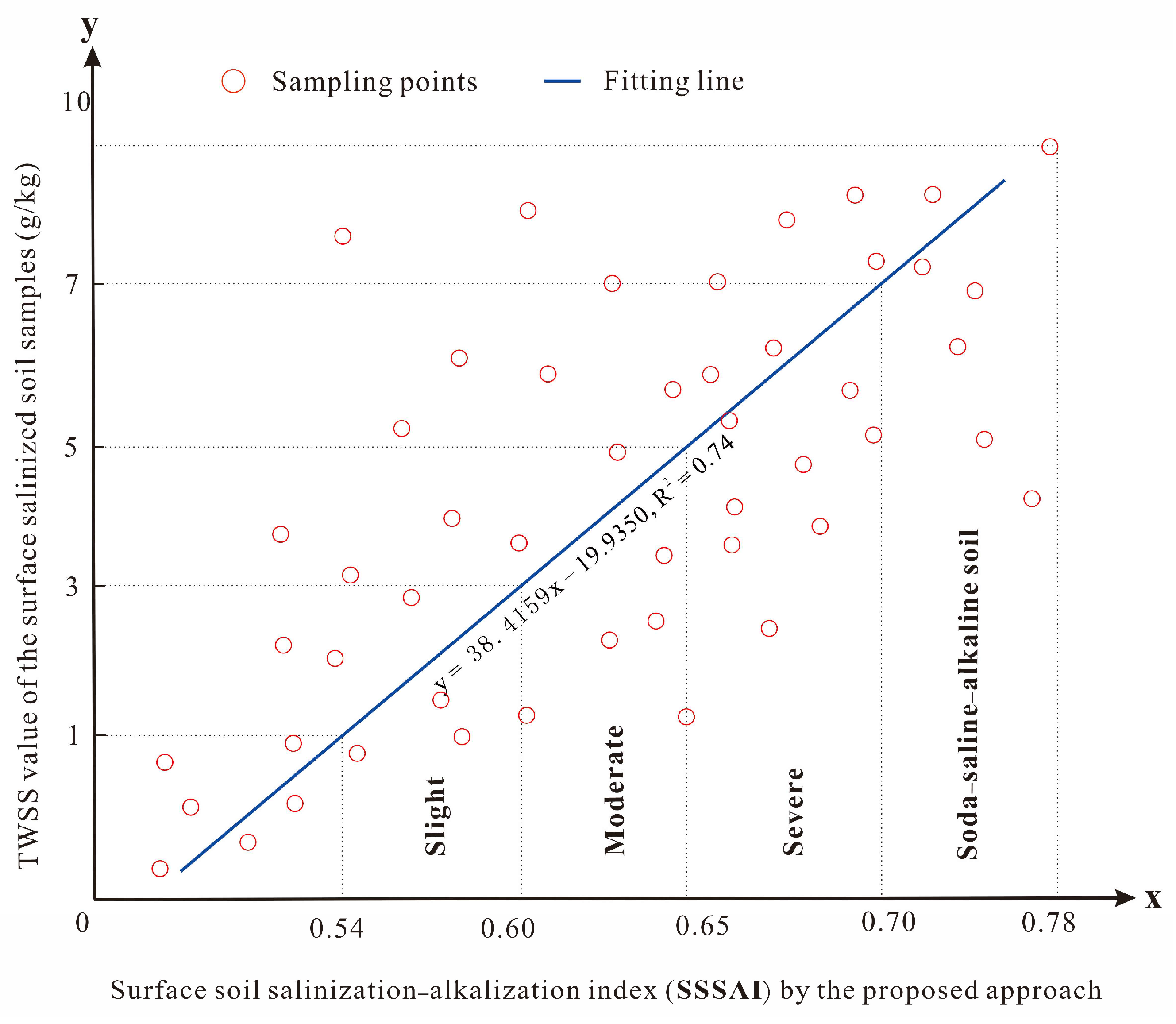
3.1. Prediction of SSS by the 3D Spectral Model and Its Accuracy

The optimal model that has the highest correlation among SSSI, 1-SSWI, and 1-VI is the combination of the ratio salt index numbered 11 in Table 3, the NDWI numbered 2 in Table 4, and the TSAVI numbered 7 in Table 5, respectively. The inversion result of SSSAI is obtained using Equation (4). The accuracy of the model is verified by the TWSS values of the 50 surface salinized soil samples within a depth of 20 cm to fit with SSSAI using weighted least-squares method, as shown in Figure 5. The fitting line shows an approximately linear relationship, and the determination coefficient of the regression model is 0.74, showing the best prediction of performance.

The inverted result obtained by the proposed approach is shown in Figure 6. Saline–alkaline regions are mainly distributed in the southwest of the study area, around puddles and rivers in the low-lying terrain. The areas of slight, moderate, severe, and soda–saline–alkaline soil with TWSS of 1~3 g/kg, 3~5 g/kg, 5~7 g/kg, and >7 g/kg, respectively, are 209 km² (51%), 116 km² (29%), 71 km² (17%), and 12 km² (3%). The Piper diagram of the 50-surface saline–alkaline soil samples in Figure 7 shows that the cations are mainly of kalium and sodium, with low percentages of magnesium and a wide range of calcium. The anions are mainly of carbonate and bicarbonate but with low percentages of sulfate and chlorate. The TWSS value is between 0.15 g/kg and 9.99 g/kg. The pH values are between 5.44 and 9.23, with a mean value of 7.85, and most values are ≥8.5.

In other words, the surface soil of the study area is characterized by saline–sodic alkalinization, mainly controlled by chemical compositions of Na⁺ + K⁺ + Ca²⁺ and HCO₃⁻ + CO₃²⁻. This inversion method can be applied in SSS estimation and monitoring for scientific policymaking according to the dynamics of saline–alkaline regions and for sustainable management of saline–alkaline land resources.

3.2. Soil Salinization–Alkalization Genesis of the Study Area

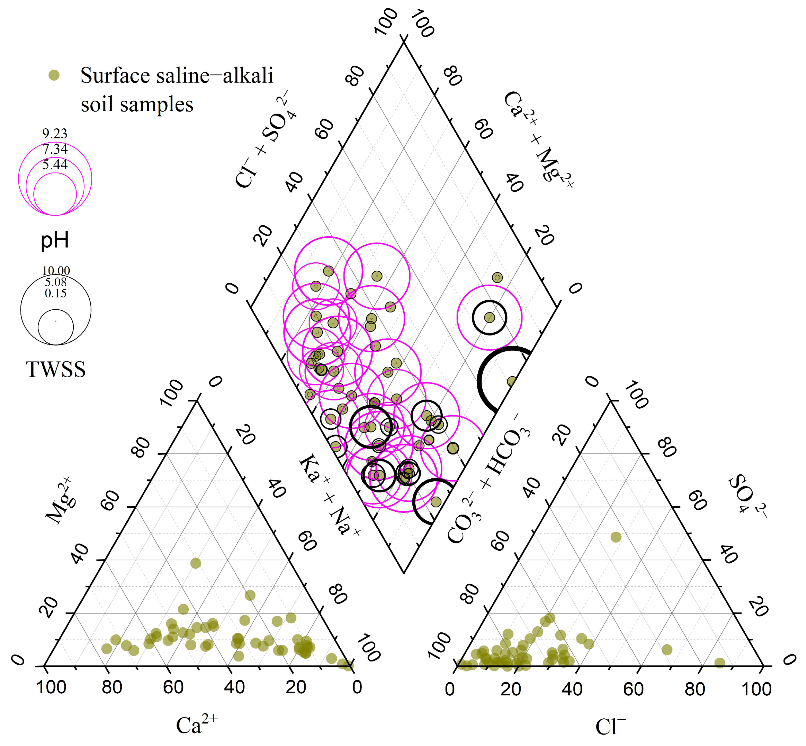
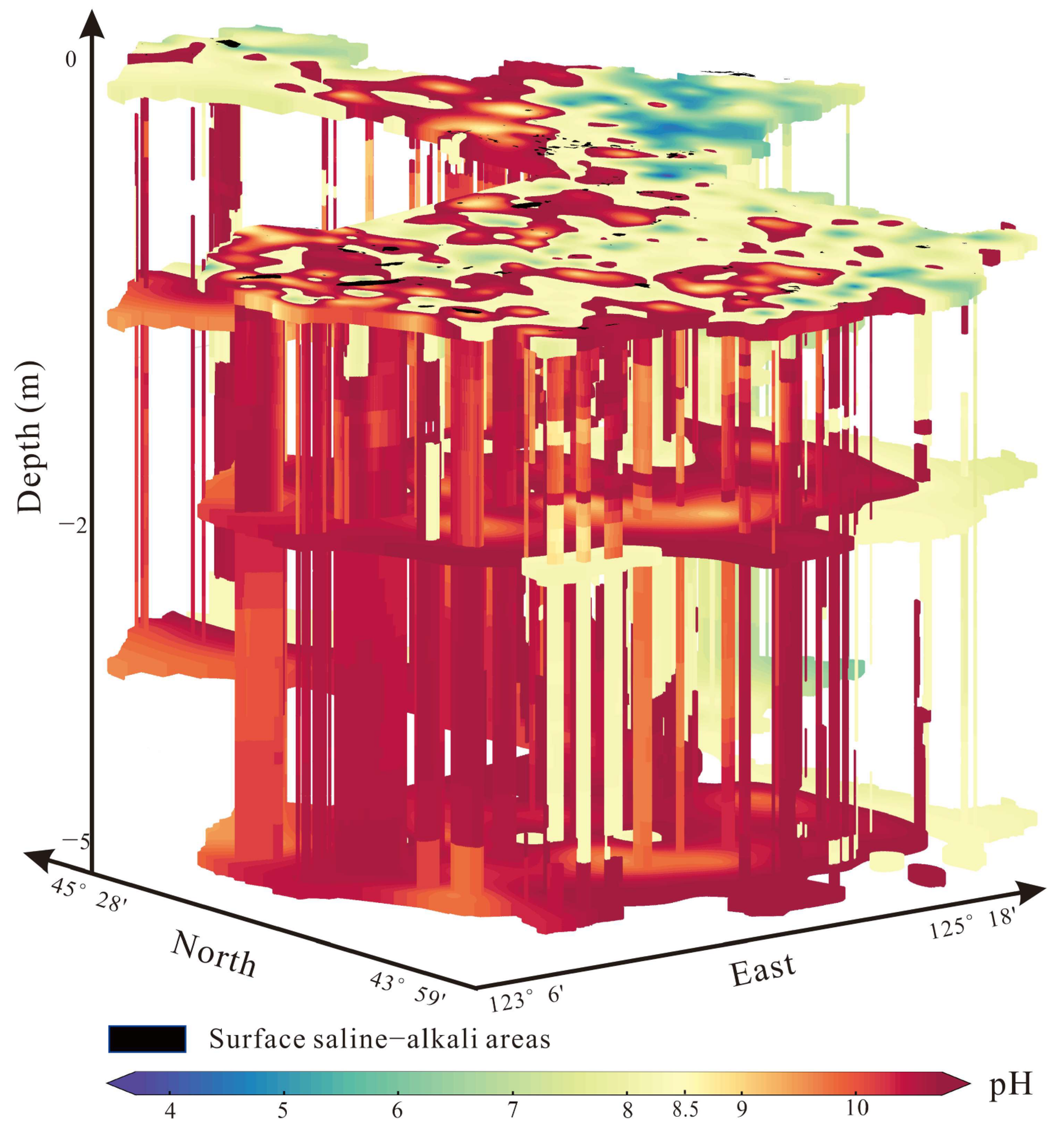
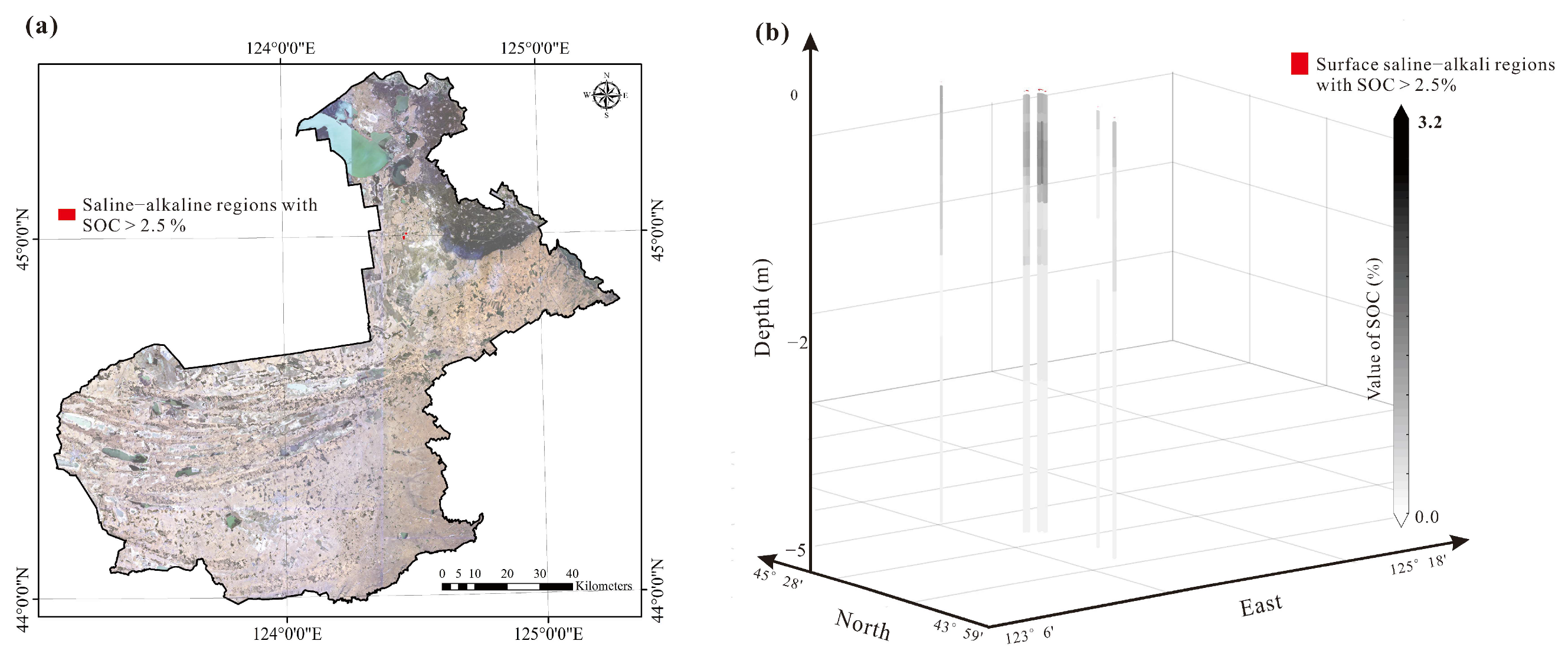
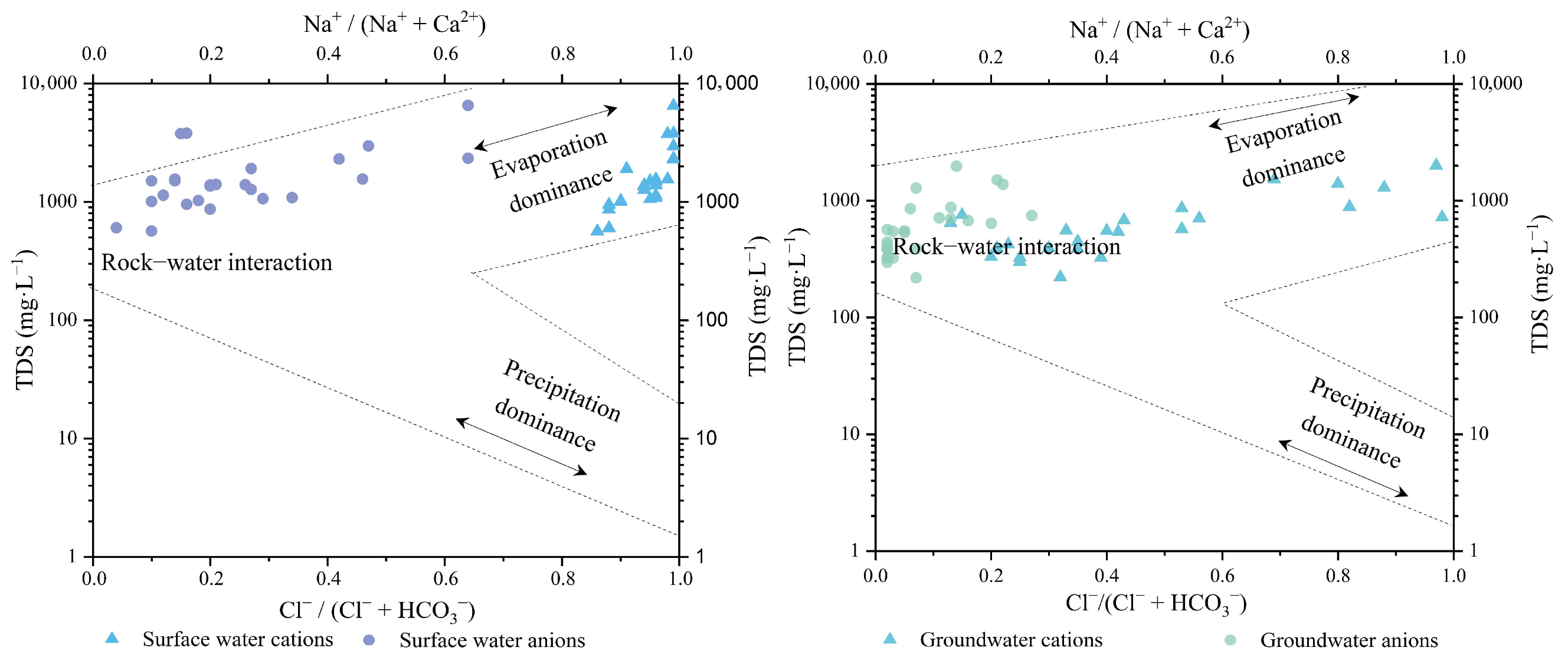
3.2.1. Origin of Salt Ions and the Deep Soil Saline–Alkaline Status

The surface water and groundwater samples were collected near the surface saline–alkaline soil samples. The cations (Ca²⁺, Mg²⁺, Na⁺, K⁺), anions (CO₃²⁻, HCO₃⁻, Cl⁻, SO₄²⁻), TDS, and pH values of these water samples were measured. The surface water Piper diagram in Figure 8 (left) shows that the cations are mainly K⁺ and Na⁺, with low percentages of Ca²⁺ and Mg²⁺. The anions are mainly CO₃²⁻ and HCO₃⁻, with low percentages of SO₄²⁻ and 0~60% Cl⁻. The groundwater Piper diagram in Figure 8 (right) shows that the cations are also mainly K⁺ and Na⁺, with low percentages of Mg²⁺, and a wide range of Ca²⁺. The anions are also mainly CO₃²⁻ and HCO₃⁻, with low percentages of Cl⁻ and SO₄²⁻. The TDS values of the surface water and groundwater are 560 mg·L⁻¹~6520 mg·L⁻¹ and 220 mg·L⁻¹~1995 mg·L⁻¹, and their pH values are 7.65~9.64 and 7.11~9.08, respectively. All the TDS values of the surface water are greater than 500 mg·L⁻¹, and this is also the case for most of the groundwater. Furthermore, most of the pH values of the surface water and groundwater are higher than 8.5. This means that the water near the surface saline–alkaline soils is unsuitable for use as drinking water. The Gibbs diagram in Figure 9 shows that the cations and anions of the samples are all dominated by evaporation and rock–water interaction [72]. The difference is that the latter has more calcium ions (Ca²⁺). In addition, the groundwater level in most of the study area is less than 5 m, so the calcium ions are brought to the surface soils, emerging as white efflorescence or crust. From the above, it can be suggested that the surface soil salt ions are carried by surface water via runoff and by groundwater via capillary rise and fluctuations. They are deposited by evaporation and aggregated in surface and subsurface soils. Alkalization mainly controlled by chemical compositions of Na⁺ + K⁺ + Ca²⁺ and HCO₃⁻ + CO₃²⁻ is a significant characteristic of surface water and groundwater.

The pH data of the 2326 deep soil samples obtained by drilling exploration were interpolated using the ordinary kriging method and classified according to the USSL (US Salinity Laboratory Staff Classification), and pH ≥ 8.5 can be categorized as alkalization [6,23]. The data are layered and arranged vertically in Figure 10, in which pH ≥ 8.5 is shown in yellow–red. The surface saline–alkaline areas are shown in black, and the soils under them are shown as vertical columns.

Thus, it can be concluded that the deep soil in the study area is mainly affected by alkalization and that the ions in the surface soda–saline–alkaline soils (including cations of Ca²⁺, Na⁺, and K⁺ and anions of CO₃²⁻ and HCO₃⁻) are from surface water and groundwater. Alkalization is the main characteristic of surface and deep soils in the study area. Its process is dominated by evaporation and soil–water interaction. This alkaline mechanism would inhibit the activity of soil microorganisms and crop growth and development and generate all kinds of toxic substances. Thus, in the farmlands of the alkaline regions, acidic fertilizers can be used as manure to decrease the alkaline intensity, especially where the pH is much higher than 8.5.

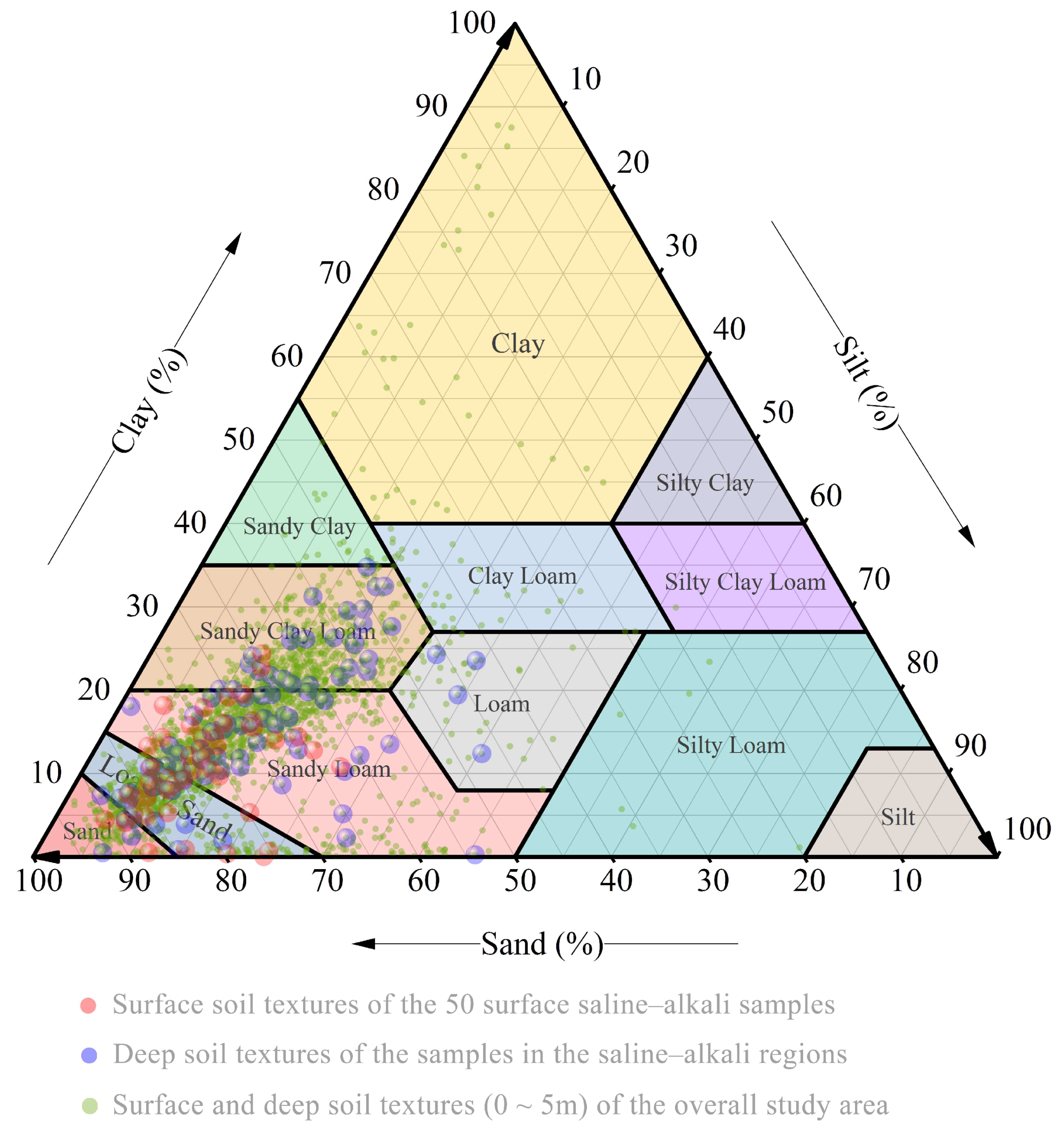
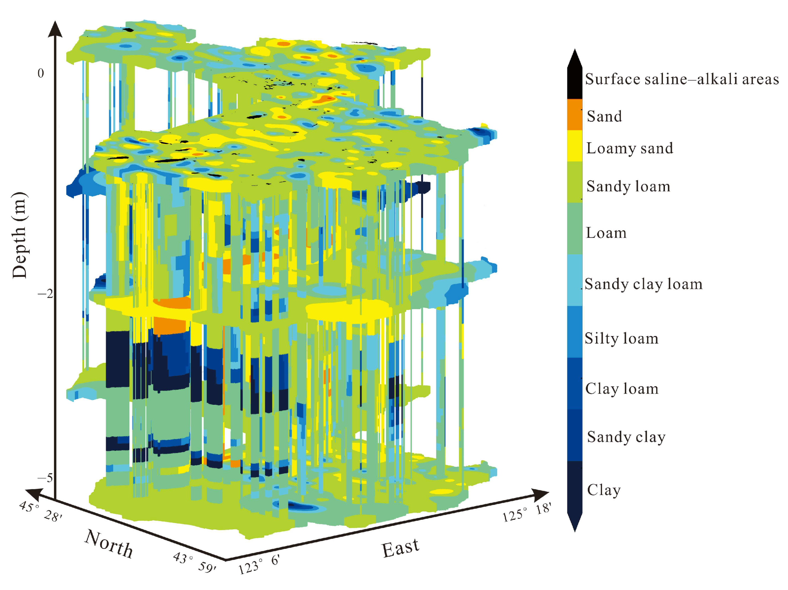
3.2.2. Surface and Deep Soil Texture Characteristics

Field survey by surface and deep soil drilling exploration have shown that salinization and alkalization are commonly distributed in the surface soils in Figure 11a and within a depth of 5 m in a drilling hole sample in the saline–alkaline areas in Figure 11b. The whitish crust or crystallization is a common phenomenon in the study area. As shown in Figure 11c, the saline–alkaline crystallization usually appears as white mesh veins or linear structures distributed along cracks in the deep soil. As the Rhino HDP adopts a hammer drilling technique to collect soil samples, each round trip of a drilling footage of one meter has its own compressibility. Thus, the actual length or depth of the soil sample is calculated using Equation (5).

$$Actual length=\frac{A}{B} ,$$

(5)

A is the length of the layered sample, B is the corresponding whole length of a drilling footage round trip, and the units are meters. White saline–alkaline crystals can be seen in the sandy soil at depths of 0~2.12 m, whereas they become weak or disappear in the clay soil between 2.12 m and 4.29 m and cannot be seen in the sandy soil between 4.29 m and 5 m.

The texture types of the surface saline–alkaline samples and deep soil samples within a depth of 5 m during drilling exploration are classified according to the USDA-NRCS soil taxonomy [73]. Herein, the percentages of clay, silt, and sand can be calculated when the weight percent of the soil particles are less than 0.002 g/kg, 0.002 g/kg~0.02 g/kg, and 0.02 g/kg~2 g/kg, respectively. Then, the types of soil textures can be classified into 12 classes, as statistically shown in Figure 12, in which the 50 types of surface saline–alkaline soil samples are mainly sandy soils (e.g., sand, loamy sand, and sandy loam) in red, while the deep soil types in saline–alkaline regions tend to be clay soils (e.g., sandy clay loam and sandy clay) in blue. The overall texture classes of the surface and deep soils (0~5 m) of the study area also consist largely of sandy–loamy soils, with a small percentage of clay soils shown in green in Figure 12. Then, the surface and deep soil textures are integrated with the surface saline–alkaline areas that are inverted using the proposed approach and spatially visualized in Figure 13. The surface saline–alkaline areas are in black on the top of the model, the soil textures of the overall study area are shown as three layers (surface, 2 m deep, and 5 m deep), and the soil textures under the surface saline–alkaline areas are shown as vertical columns. It can be clearly seen that the surface or subsurface soils are mainly sandy–loamy soils in yellow–green, while the types of deep soil textures under the surface saline–alkaline areas are mainly characterized as sandy or loamy soils interbedded with clay soils in cyan–blue. The sandy soils are conducive to the infiltration of water and the corresponding downward migration–dilution of salt ions, in which the moisture evaporates easily to leave the salt ions on the soil surface and subsurface. The multi-layer clay soils (in cyan–blue) have a hindering effect on the infiltration and migration action, where significant white crusts are usually fostered above them, and minimal or no whitish efflorescence can be seen below them. Therefore, the clay layers serve as interrupted aquifers, and such vertical distribution of the soil textures provides a good environment for the accumulation of salt ions to form saline–alkaline soils in the study area. In the multilayer clay soil regions where the terrain is low and the surface–subsurface soil is sandy, the soils become easily waterlogged, and they are used for water-absorbent crops (e.g., paddy rice, maize, and the like).

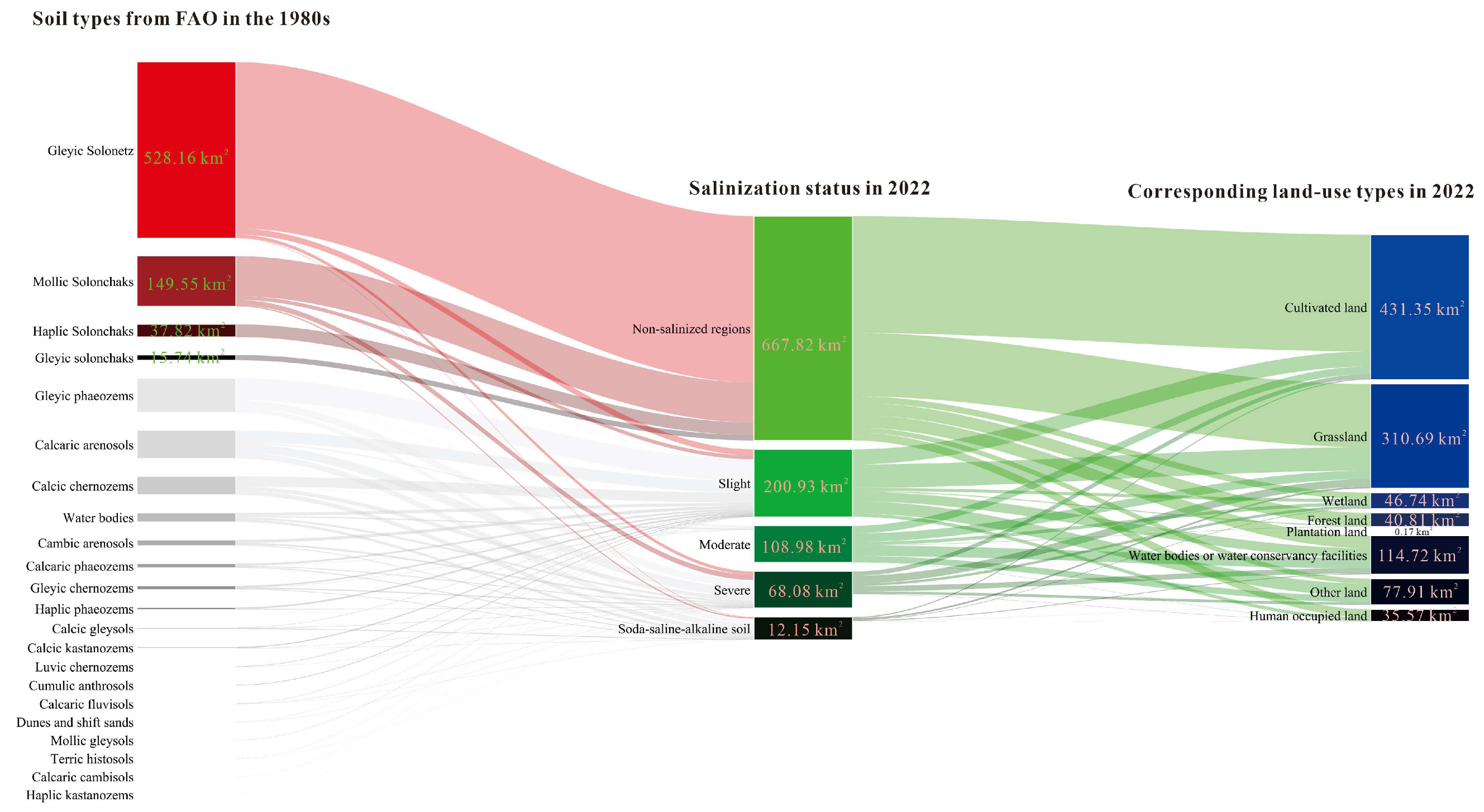
3.3. Changes in the Saline–Alkaline Status from the 1980s to 2022 and Land-Use Management Suggestions for the Alkaline Soils

The FAO HWSD v1.2 soil database provided the detailed soil types of the study area and was obtained from the Office for the Second National Soil Survey of China in the 1980s (from 1979 to 1985) at a scale of 1:1 million and a resolution of 30 arc-seconds, in which the total area of the saline–alkaline soils in Figure 1 was 731.26 km² (i.e., gleyic solonetz 528.16 km², gleyic solonchaks 15.74 km², haplic solonchaks 37.82 km², and mollic solonchaks 149.55 km²). The saline–alkaline region in 2022 in Figure 6, inverted using the proposed 3D spectral space optimization method in this research, was 390.14 km² (i.e., slight 200.93 km², moderate 108.98 km², severe 68.08 km², and soda–saline–alkaline soil 12.15 km²). The changes between the 1980s and 2022 are shown as a Sankey diagram in Figure 14. It can be estimated that the saline–alkaline area decreased by about 341.12 km² during these forty years, during which a large portion of the gleyic solonetz and mollic solonchaks became non-salinized, and the saline–alkaline status in 2022 was mainly descended from other types of soils (e.g., calcaric arenosols, calcaric cambisols, calcaric fluvisols, calcaric phaeozems, calcic chernozems, and the like). These saline–alkaline soils were mainly used as cultivated land, grassland, waterbodies, or water conservancy facilities in 2022.

According to the FAO World reference base (WRB) for soil resources, which was updated in 2015 [74], soil can be considered a mollic horizon that is conducive to crop cultivation when the SOC content at 20 cm depth is greater than 2.5%. Furthermore, it was proven that saline–alkaline soils show better productivity and are more capable of producing rice and wheat crops compared with non-salinized soils if they are properly managed according to their properties [75,76]. In this way, we found an area of about 0.95 km² of mollic horizon in the saline–alkaline regions, as shown in Figure 15a. The corresponding deep soil SOC distribution is shown in Figure 15b, from which it can be seen that the SOC content was higher in the surface–subsurface soil within 2 m than in the deeper soils at 2~5 m, and in which 0.75 km² is state-owned unused land. The inverted saline–alkaline status of its deep soil SOC and pH is statistically shown in Figure 16, in which most of the pH values are higher than 8.5 when the SOC < 2.5%. Thus, this unutilized region is of weak alkalinization and high SOC (>2.5%), and it is suggested to be used for cultivation (e.g., paddy rice, wheat crops, and the like). Regions of saline–alkaline unused land, where the surface SOC is much lower than 2.5% but the deep soil SOC is much higher than 2.5%, can be used for deep-rooted plants (e.g., grapevines, apple trees, and the like). The regions of low SOC of the entire soil profile are suggested to be less tilled or no-tillage. This method of utilization of the salinized unused land is significant because the saline–alkali land is also a kind of important land resource, especially for China with its large population and little available farmland per capita.

4. Discussions

4.1. Uncertainty of Predicting SSS Using the Proposed Method and Grading of the Soil Salinity of the Study Area

The 3D spectral Model is based on the correlation between the indicators SSSI-SSWI and SSSI-VI being negative, while SSWI-VI is positive. This is because increasing soil wetness can decrease soil salinity and increasing soil salinity can restrain the growth of vegetation. The more moisture the soil has, the more beneficial it is to vegetation growth. However, these relations are sometimes weak, especially in the following cases. Firstly, when the study area is covered by vegetation or dominated by salt-tolerant plants, the relationship between SSSI and VI may be unclear because soils covered by thick vegetation cannot be detected using multispectral satellite imagery. Salt-tolerant plants are immune to salinity and can flourish regardless of salinization–alkalization [8]. Secondly, when the indices for soil salinity inversion are composited by visible bands, it may be hard to find the optimal model using this method and it may be inaccurate. As the visible-band reflectance characteristics of saline soils are extremely dependent on moisture conditions, the increase in soil moisture will reduce the soil surface reflectance. This can dilute the salts and make the white crusts of salinized soils darker in true color imagery, which reduces the overall surface reflectance [77]. On the other hand, the drier the soils, the more salts are crystallized and precipitation on their surfaces. Therefore, the indices used by this model are usually the ones composited by the NIR-SWIR bands because they are less affected by soil wetness and it is easier to distinguish soil salinity from vegetation and soil wetness. Thirdly, the masking of water bodies is also a necessary step because the proposed 3D spectral model cannot leave the water bodies out. In addition, timescale and spatial resolution have to be considered during soil salinity inversion and investigation because it is a dynamic process [39]. The distribution and intensity may vary significantly at different times or during winter or summer, strong rainfall, or sunny weather, and the like. In this regard, different inversion results could be obtained for different periods of time and spatial scales.

According to the definition of saline–alkaline soils, a soil in which the amounts of soluble salts in the root-zone are sufficiently high enough to impair the growth of crop plants is considered to be saline–alkaline soil [3,4,5,6,7,8]. However, because salt injuries depend heavily on species, variety, plant growth stage, environmental factors, and the type of salt, there are many ways to classify it, and it is very difficult to precisely define [6]. The conventional methods used to quantify soil salinity and sodicity were conducted through the measurement of electrical conductivity (EC) and pH and calculation of the exchangeable sodium percentage (ESP) using Equation (6) [6,23], which was first suggested by the United States Salinity Laboratory Staff in 1954 (USSL Staff), as in

Table 6. The frequently used taxonomies for soil salinity–sodicity classification.

Taxonomies	Indicators	Saline–Alkaline Classification/Grading
USSL Staff 1954	EC*, ESP, pH	EC* ≥ 4, ESP < 15%, pH < 8.5	saline
		EC* ≥ 4, ESP ≥ 15%, pH ≥ 8.5	saline–sodic
		EC* < 4, ESP ≥ 15%, pH > 8.5	sodic
FAO 1988	EC*	0 ≤ EC* < 2	non-saline
		2 ≤ EC* < 4	slightly saline
		4 ≤ EC* < 8	moderately saline
		8 ≤ EC* < 16	strongly saline
		16 ≤ EC*	very strongly saline
USDA 2002	EC*	0 ≤ EC* < 2	non-saline
		2 ≤ EC* < 4	very slightly saline
		4 ≤ EC* < 8	slightly saline
		8 ≤ EC* < 16	moderately saline
		16 ≤ EC*	strongly saline
CTNSS 2022	TWSS	1 k·kg−1 ≤ TWSS < 3 k·kg−1	slightly saline
		3 k·kg−1 ≤ TWSS < 5 k·kg−1	moderately saline
		5 k·kg−1 ≤ TWSS < 7 k·kg−1	strongly saline
		7 k·kg−1 ≤ TWSS	sodic saline

EC* is measured at 25 °C and its unit is Deci Siemens per meter (dS·m⁻¹) [42].

. But it was time-energy consuming and inconvenient to obtain EC, ESP, and pH data within the same short period of time. As a result, the commonly used taxonomy for soil salinity and sodicity grading was via EC, as proposed by [78] of the Food and Agriculture Organization (FAO) classification system in 1988 and by [79] of the United States Department of Agriculture (USDA) classification method in 2002.

$$ESP=\frac{\left[100-\left(-0.0126+0.01475\times SAR\right)\right]}{[1+(-0.0126+0.01475\times SAR\left)\right]}, \mathrm{in} \mathrm{which} SAR=\frac{{\mathrm{N}\mathrm{a}}^{+}}{\sqrt{0.5\times ({\mathrm{C}\mathrm{a}}^{2+}+{\mathrm{M}\mathrm{g}}^{2+})}}$$

(6)

In this study, the grading method by CTNSS standard is applied, which was enacted according to the different regions’ climate and the different saline–alkaline types in China. In a subhumid climate where the salinization is soda-based (CO₃²⁻ + HCO₃⁻ > Cl⁻ + SO₄²), grading of TWSS can be carried out by CTNSS 2022, as listed in Table 6. Samples for measuring TWSS should be collected within depths of 0~20 cm. In arid regions and coastal areas, the grading of salinity varies greatly in response to saline–alkaline soil type and depth, and samples of the former should be taken at depths of 0~30 cm and the latter at a depth of 1 m.

However, these taxonomies do not make it clear how the thresholds were decided and how the different levels of saline–alkaline soils affect the growth of plants and creatures on them (such as the height and stem diameter of the crop plants, their total organic carbon contents, and their grain yield). But a linear relationship was commonly recognized between soil salinity and crop yield, whereby the output would decrease linearly with increasing salinity beyond threshold levels [80]. Our field survey also found that the growth of local crops and vegetation was negatively affected by the salinization-alkalization mechanism when the length (or height) was low, the leaves were burnt, the fruits were shriveled and not full, and the like. The method of grading of the salinity using CTNSS 2022 is dependent upon the objective difference of climates and salinization–alkalization types. TWSS measured by field survey and laboratory analysis is incorporated with RS inversion using the proposed 3D spectral space optimization method, which makes it practical to conduct RS saline–alkaline mapping at a national scale in China and provides an approach for assessing the degree of salinization–alkalization for the green and sustainable development of saline–alkaline land resources.

4.2. The Depth of Soil Salinization and Alkalization of the Study Area

Salinity is usually closely related to groundwater depth, and it is also dynamic. Some researchers proposed that salinization or alkalization occurred when the groundwater depth was less than 2.0 m and the salinity was higher than 0.48 dS·m⁻¹. For groundwater with lower salinity, the groundwater table should not be shallower than 1.5 m [81,82]. It was found that soil salinization continued and was aggravated when the water table reached 5 m, and the shallow groundwater level has already exceeded the critical water level (2–3 m) in the study area [83]. The most recent FAO Global Map of Salt-Affected Soils (GSASmap) mapped the global soil salinity at two intervals of topsoil (0–30 cm) and subsoil (30–100 cm), with measurements covering 118 countries and 424 million hectares of topsoil and 833 million hectares of subsoil [84]. This study conducted the field investigation and developed the deep soil saline–alkaline model using a depth of 5 m because we thought that the crop plants (like shallow-rooted annual crops or deep-rooted trees) have different root depths in saline–alkaline areas, according to the definition of soil salinization and alkalization. In shallow water-table regions, the roots of plants are often also shallow, and vice versa. In this way, salinization and alkalization in shallow water-table regions will also be concentrated on the surface and in the shallow subsurface, while in deep water-table regions, they cannot reach that deep because of the interrupted aquifers, strong evaporation, and the like. Therefore, the depth of 5 m for soil salinity investigation was adopted and pH data were applied to build the 3D alkalization model. The plot in Figure 16 of the pH–SOC relationship of the samples under the inverted saline–alkaline regions displays a weak descending trend (or an inverse relationship) and shows that many of the samples are concentrated in the region (pH > 8.5 and SOC < 2.5%), which means that the salinization–alkalization mechanism affects the accumulation of SOC in the soils within a depth of 5 m. Thus, usage of the saline–alkaline land resources should be decided upon, and different land-use policies should be applied according to depth for scientific and sustainable development.

4.3. Genesis of Soil Salinization and Alkalization of the Study Area

It was acknowledged that soil salinization–alkalization was usually induced by many factors, which included soil types and land use types, topography and landforms, climate conditions (such as annual mean temperature, annual mean precipitation, etc.), surface evaporation and plant transpiration, brackish and saline irrigation water, restricted drainage and a rising water-table, and other anthropogenic activities (like overuse of fertilizers, use of sewage sludge or treated sewage effluent, and dumping of industrial brine) [2,3,4,5,6,7,8,85]. The soil salinization–alkalization problem of the study area is also affected by these factors. However, according to the field investigation and results obtained by this study, the saline–alkaline problem is mainly induced by the conditions that the annual mean evaporation is higher than the annual mean precipitation, the groundwater level rises in the summer–autumn seasons and brings the salt ions to the surface–subsurface soils, and the clay soils as interrupted aquifers prevent salt ions from leaching or infiltrating into the deep underground. Meanwhile, the freeze–thaw action in the winter–spring seasons and irrigation by groundwater (especially in the east of the study area with high terrain and a deep water-table) from anthropogenic activities make it worse. A schematic diagram of this process is illustrated in Figure 17.

In general, utilization of the saline–alkaline soils or land resources should be decided based on their degree and properties (pH, SOC, textures, depth, terrain, water table, and so on). In the west of the study area, low-lying terrains that are usually dominated by the twin menace of waterlogging and salinization instead of a single effect, the adoption of salt- and waterlogging-tolerate crops is suggested in the meantime to bring down the water table to a safe limit and prevent further increase. Installation of a drainage system could also be considered to facilitate agricultural activities. In the east of the study area, which has a high terrain and deep water-table level and salinization–alkalization is mainly induced by human factors (or secondary salinization) in this region, reducing saline water irrigation and the overuse of saline–alkaline-vulnerable fertilizers would be a better option.

5. Conclusions

This study proposed an SSSI-SSWI-VI 3D spectral space optimization method for SSS inversion, combined with field verification and deep soil investigation. The results are as follows: (1) The optimization method using the SSSI-SSWI-VI 3D spectral model is effective in SSS inversion, with a determination coefficient R² of 0.74. It can be applied to estimate soil salinity, whether the soils are bare and dry or wet and covered by vegetation to an extent. (2) Sodic alkalization of Na⁺ + K⁺ + Ca²⁺ and HCO₃⁻ + CO₃²⁻ is identified as the main problem in the surface and deep soils in the study area. (3) The deep clay soils inhibit the water and salt ions from penetrating them and restrain the associated infiltration and dilution action. This is the cause of deep soil salinization–alkalization in the study area. (4) The saline–alkaline mechanism has an inverse effect on deep soil SOC accumulation, but saline–alkaline land resources could be utilized sustainably and effectively according to their properties. There is an alkaline region with SOC content greater than 2.5%, and this may be suitable for future cultivation.

Regarding the limitations of the study, our future work will clarify the basis and principles of the relationship between the thresholds of grading and the associated effect on crop plants and creatures, provide detailed evidence of the deep soil saline–alkaline penetration depth, and investigate the multifactor operation mechanism of saline–alkaline induction.

References

1. Ivushkin, K.; Bartholomeus, H.; Bregt, A.K.; Pulatov, A.; Kempen, B.; de Sousa, L. Global mapping of soil salinity change. Remote Sens. Environ. 2019, 231, 111260. [Google Scholar] [CrossRef]
2. FAO. The State of the World’s Land and Water Resources for Food and Agriculture—Systems at Breaking Point; Synthesis Report; Food and Agriculture Organization of the United Nations: Rome, Italy, 2021; pp. 10–14. [Google Scholar]
3. FAO. Salt-Affected Soils. Available online: http://www.fao.org/soils-portal/soil-management/management-of-some-problem-soils/salt-affected-soils/more-information-on-salt-affected-soils/en/ (accessed on 12 January 2024).
4. Al-Khaier, F. Soil Salinity Detection Using Satellite Remote Sensing. Master’s Thesis, International Institute for Geo-information Science and Earth Observation, Enschede, The Netherlands, 2003. [Google Scholar]
5. Wallender, W.W.; Tanji, K.K. Agricultural Salinity Assessment and Management, 2nd ed.; American Society of Civil Engineers: Reston, VA, USA, 2011; pp. 1–1069. [Google Scholar]
6. Zamann, M.; Shahidd, S.A.; Heng, L. Guideline for Salinity Assessment, Mitigation and Adaptation Using Nuclear and Related Techniques; Springer Open: Vienna, Austria, 2018; pp. 1–162. [Google Scholar]
7. Hopmans, J.W.; Qureshi, A.S.; Kisekka, I.; Munns, R.; Grattan, S.R.; Rengasamy, P.; Ben-Gal, A.; Assouline, S.; Javaux, M.; Minhas, P.S.; et al. Critical knowledge gaps and research priorities in global soil salinity. Adv. Agron. 2021, 169, 1–156. [Google Scholar]
8. Li, X.; Li, Y.; Wang, B.; Sun, Y.; Cui, G.; Liang, Z. Analysis of spatial-temporal variation of the saline-sodic soil in the west of Jilin Province from 1989 to 2019 and influencing factors. Catena 2022, 217, 106492. [Google Scholar] [CrossRef]
9. Yang, F.; An, F.; Ma, H.; Wang, Z.; Zhou, X.; Liu, Z. Variations on soil salinity and sodicity and its driving factors analysis under microtopography in different hydrological conditions. Water 2016, 8, 227. [Google Scholar] [CrossRef]
10. Clark, R.N.; King, T.V.V.; Klejwa, M.; Swayze, G.A.; Vergo, N. High spectral resolution reflectance spectroscopy of minerals. J. Geophys. Res. 1990, 95, 12653–12680. [Google Scholar] [CrossRef]
11. Metternicht, G.; Zinck, J.A. Spatial discrimination of salt- and sodium-affected soil surfaces. Int. J. Remote Sens. 1997, 18, 2571–2586. [Google Scholar] [CrossRef]
12. Khan, N.M.; Rastoskuev, V.v.; Sato, Y.; Shiozawa, S. Assessment of hydrosaline land degradation by using a simple approach of remote sensing indicators. Agric. Water Manag. 2005, 77, 96–109. [Google Scholar] [CrossRef]
13. Douaoui, A.E.K.; Nicolas, H.; Walter, C. Detecting salinity hazards within a semiarid context by means of combining soil and remote-sensing data. Geoderma 2006, 134, 217–230. [Google Scholar] [CrossRef]
14. Bannari, A.; Guedon, A.M.; El-Harti, A.; Cherkaoui, F.Z.; El-Ghmari, A. Characterization of slightly and moderately saline and sodic soils in irrigated agricultural land using simulated data of advanced land imaging (EO-1) sensor. Commun. Soil Sci. Plan. 2008, 39, 2795–2811. [Google Scholar] [CrossRef]
15. Bouaziz, M.; Matschullat, J.; Gloaguen, R. Improved remote sensing detection of soil salinity from a semi-arid climate in Northeast Brazil. Comptes Rendus Geosci. 2011, 343, 795–803. [Google Scholar] [CrossRef]
16. Allbed, A.; Kumar, L.; Sinha, P. Soil salinity and vegetation cover change detection from multi-temporal remotely sensed imagery in Al Hassa Oasis in Saudi Arabia. Geocarto Int. 2018, 33, 830–846. [Google Scholar] [CrossRef]
17. Abuelgasim, A.; Ammad, R. Mapping soil salinity in arid and semi-arid regions using Landsat 8 OLI satellite data. Remote Sens. Appl. 2019, 13, 415–425. [Google Scholar] [CrossRef]
18. Tran, T.v.; Tran, D.X.; Myint, S.W.; Huang, C.; Pham, H.V.; Luu, T.H.; Vo, T.M.T. Examining spatiotemporal salinity dynamics in the Mekong River Delta using Landsat time series imagery and a spatial regression approach. Sci. Total Environ. 2019, 687, 1087–1097. [Google Scholar] [CrossRef] [PubMed]
19. Zewdu, S.; Suryabhagavan, K.V.; Balakrishnan, M. Geo-spatial approach for soil salinity mapping in Sego Irrigation Farm, South Ethiopia. J. Saudi Soc. Agric. Sci. 2017, 16, 16–24. [Google Scholar] [CrossRef]
20. Suweis, S.; Rinaldo, A.; van der Zee, S.E.A.T.M.; Daly, E.; Maritan, A.; Porporato, A. Stochastic modeling of soil salinity. Geophys. Res. Lett. 2010, 37, 1–5. [Google Scholar] [CrossRef]
21. Perri, S.; Molini, A.; Hedin, L.O.; Porporato, A. Contrasting effects of aridity and seasonality on global salinization. Nat. Geosci. 2022, 15, 375–381. [Google Scholar] [CrossRef]
22. Bian, J.; Tang, J.; Lin, N. Relationship between saline-alkali soil formation and neotectonic movement in Songnen Plain, China. Environ. Geol. 2008, 55, 1421–1429. [Google Scholar] [CrossRef]
23. Salcedo, F.P.; Cutillas, P.P.; Cabañero, J.J.A.; Vivaldi, A.G. Use of remote sensing to evaluate the effects of environmental factors on soil salinity in a semi-arid area. Sci. Total Environ. 2022, 815, 152524. [Google Scholar] [CrossRef]
24. Yan, Y.; Kayem, K.; Hao, Y.; Shi, Z.; Zhang, C.; Peng, J.; Liu, W.; Zuo, Q.; Ji, W.; Li, B. Mapping the Levels of Soil Salination and Alkalization by Integrating Machining Learning Methods and Soil-Forming Factors. Remote Sens. 2022, 14, 3020. [Google Scholar] [CrossRef]
25. Zhang, Y.; Hou, K.; Qian, H.; Gao, Y.; Fang, Y.; Xiao, S.; Tang, S.; Zhang, Q.; Qu, W.; Ren, W. Characterization of soil salinization and its driving factors in a typical irrigation area of Northwest China. Sci. Total Environ. 2022, 837, 155808. [Google Scholar] [CrossRef]
26. Everitt, J.H.; Escobar, D.E.; Gerbermann, A.H. Detecting saline soils with video imagery. Photogramm. Eng. Remote Sens. 1988, 54, 1283–1287. [Google Scholar]
27. Peñuelas, J.; Isla, R.; Filella, I.; Araus, J.L. Visible and near-infrared reflectance assessment of salinity effects on barley. Crop Sci. 1997, 37, 198–202. [Google Scholar] [CrossRef]
28. Fernandez-Buces, N.; Siebe, C.; Cram, S.; Palacio, J. Mapping soil salinity using a combined spectral response index for bare soil and vegetation: A case study in the former lake Texcoco, Mexico. J. Arid Environ. 2006, 65, 644–667. [Google Scholar] [CrossRef]
29. Zhang, T.T.; Zeng, S.L.; Gao, Y.; Ouyang, Z.T.; Li, B.; Fang, C.M.; Zhao, B. Using hyperspectral vegetation indices as a proxy to monitor soil salinity. Ecol. Indic. 2011, 11, 1552–1562. [Google Scholar] [CrossRef]
30. Elmetwalli, A.M.H.; Tyler, A.N.; Hunter, P.D.; Salt, C.A. Detecting and distinguishing moisture-and salinity-induced stress in wheat and maize through in situ spectroradiometry measurements. Remote Sens. Lett. 2012, 3, 363–372. [Google Scholar] [CrossRef]
31. Allbed, A.; Kumar, L.; Aldakheel, Y.Y. Assessing soil salinity using soil salinity and vegetation indices derived from IKONOS high-spatial resolution imageries: Applications in a date palm dominated region. Geoderma 2014, 230–231, 1–8. [Google Scholar] [CrossRef]
32. Farifteh, J.; Farshad, A.; George, R.J. Assessing salt-affected soils using remote sensing, solute modelling, and geophysics. Geoderma 2006, 130, 191–206. [Google Scholar] [CrossRef]
33. Li, H.Y.; Shi, Z.; Webster, R.; Triantafilis, J. Mapping the three-dimensional variation of soil salinity in a rice-paddy soil. Geoderma 2013, 195–196, 31–41. [Google Scholar] [CrossRef]
34. Liu, G.; Li, J.; Zhang, X.; Wang, X.; Lv, Z.; Yang, J.; Shao, H.; Yu, S. GIS-mapping spatial distribution of soil salinity for Eco-restoring the Yellow River Delta in combination with Electromagnetic Induction. Ecol. Eng. 2016, 94, 306–314. [Google Scholar] [CrossRef]
35. Jiang, Q.; Peng, J.; Biswas, A.; Hu, J.; Zhao, R.; He, K.; Shi, Z. Characterising dryland salinity in three dimensions. Sci. Total Environ. 2019, 682, 190–199. [Google Scholar] [CrossRef]
36. Dehni, A.; Kheloufi, N.; Bouakkaz, K. Implicit modeling of salinity reconstruction by using 3D combined models. Environ. Earth Sci. 2020, 79, 440. [Google Scholar] [CrossRef]
37. FAO. Harmonized World Soil Database v12. Available online: https://www.fao.org/soils-portal/soil-survey/soil-maps-and-databases/harmonized-world-soil-database-v12/en/ (accessed on 12 January 2024).
38. Qin, Y.; Bai, Y.; Chen, G.; Liang, Y.; Li, X.; Wen, B.; Lu, X.; Li, X. The effects of soil freeze–thaw processes on water and salt migrations in the western Songnen Plain, China. Sci. Rep. 2021, 11, 3888. [Google Scholar] [CrossRef] [PubMed]
39. Han, Y.; Ge, H.; Xu, Y.; Zhuang, L.; Wang, F.; Gu, Q.; Li, X. Estimating Soil Salinity Using Multiple Spectral Indexes and Machine Learning Algorithm in Songnen Plain, China. IEEE J. Sel. Top. Appl. Earth Obs. Remote Sens. 2023, 16, 7041–7050. [Google Scholar]
40. Yu, H.; Wang, Z.; Mao, D.; Jia, M.; Chang, S.; Li, X. Spatiotemporal variations of soil salinization in China’s West Songnen Plain. Land Degrad. Dev. 2023, 34, 2366–2378. [Google Scholar] [CrossRef]
41. Li, P. Soil Analysis in Xinjiang; People’s Publishing House in Xinjiang: Urumqi, China, 1983; pp. 1–207. (In Chinese) [Google Scholar]
42. Richards, L.A. Diagnosis and Improvement of Saline and Alkali Soils; United States Salinity Laboratory Staff: Washington, DC, USA, 1954; pp. 8–17. [Google Scholar]
43. Page, A.L.; Miller, R.H.; Jeeney, D.R. Methods of soil analysis, part 2. In Chemical and Mineralogical Properties; Soil Science Society of American Publication: Madison, WI, USA, 1992; p. 1159. [Google Scholar]
44. Bao, S.D. Soil and Agricultural Chemistry Analysis; China Agriculture Press: Beijing, China, 2000; pp. 1–495. (In Chinese) [Google Scholar]
45. Eaton, A.D.; Clesceri, L.S.; Rice, E.W.; Greenberg, A.E. Standard Methods for the Examination of Water and Wastewater, 21st ed.; APHA Publication: Washington, DC, USA, 2005. [Google Scholar]
46. Thomas, G.W. Soil pH and soil acidity. In Methods of Soil Analysis, Part III, 3rd ed.; Sparks, D.L., Ed.; American Society of Agronomy: Madison, WI, USA, 1996; pp. 475–490. [Google Scholar]
47. Baver, L.; David, L. Soil Physics, 3rd ed.; Wiley: New York, NY, USA, 1956. [Google Scholar]
48. Teng, S.C.; Hsai, C.C.; Hseung, Y. hydrometer method of mechanical analysis of soils. ACTA Pedol. Sin. 1958, 6, 70–83. [Google Scholar]
49. Gao, J.J.; Liu, J.H.; Zou, J.J.; Song, X.H.; Zhu, A.M. Determination of Dissolved Organic Carbon in Seawater by Combustion Oxidation-non-dispersive Infrared Absorption Method. Adv. Mar. Sci. 2009, 27, 477–482. (In Chinese) [Google Scholar]
50. Gilmore, K.R.; Luong, H.V. Improved method for measuring total dissolved solids. Anal. Lett. 2016, 49, 1772–1782. [Google Scholar] [CrossRef]
51. Maiorova, A.V.; Belozerova, A.A.; Mel’chakov, S.Y.; Mashkovtsev, M.A.; Suvorkina, A.S.; Shunyaev, K.Y. Determination of Arsenic and Antimony in Ferrotungsten by Inductively Coupled Plasma Atomic Emission Spectrometry. J. Anal. Chem. 2019, 74, 18–26. [Google Scholar] [CrossRef]
52. Pohl, P.; Stecka, H.; Jamroz, P. Solid phase extraction with flame atomic absorption spectrometry for determination of traces of Ca, K, Mg and Na in quality control of white sugar. Food Chem. 2012, 130, 441–446. [Google Scholar] [CrossRef]
53. Hodge, E.M.; Martinez, P.; Sweetin, D. Determination of inorganic cations in brine solutions by ion chromatography. J. Chromatogr. A 2000, 884, 223–227. [Google Scholar] [CrossRef]
54. Abd El-Hamid, H.T.; Alshehri, F.; El-Zeiny, A.M.; Nour-Eldin, H. Remote sensing and statistical analyses for exploration and prediction of soil salinity in a vulnerable area to seawater intrusion. Mar. Pollut. Bull. 2023, 187, 114555. [Google Scholar] [CrossRef] [PubMed]
55. Tripathi, N.K.; Brijesh, K.R.; Dwivedi, P. Spatial modelling of soil alkalinity in GIS environment using IRS data. In Proceedings of the 18th Asian Conference in Remote Sensing, Kuala Lumpur, Malaysia, 20–24 October 1997. [Google Scholar]
56. Amalo, L.F.; Hidayat, R.; Sulma, S. Analysis of Agricultural Drought in East Java Using Vegetation Health Index. AGRIVITA J. Agric. Sci. 2018, 40, 63–73. [Google Scholar] [CrossRef]
57. Abbas, A.; Khan, S. Using remote sensing techniques for appraisal of irrigated soil salinity. In Proceedings of the International Congress on Modelling and Simulation, Land, Water and Environmental Management: Integrated Systems for Sustainability, Christchurch, New Zealand, 10–13 December 2007. [Google Scholar]
58. Abbas, A.; Khan, S.; Hussain, N.; Hanjra, M.A.; Akbar, S. Characterizing soil salinity in irrigated agriculture using a remote sensing approach. Phys. Chem. Earth 2013, 55–57, 43–52. [Google Scholar] [CrossRef]
59. Scudiero, E.; Skaggs, T.H.; Corwin, D.L. Regional scale soil salinity evaluation using Landsat 7, Western San Joaquin Valley, CA, USA. Geoderma Reg. 2014, 2–3, 82–90. [Google Scholar] [CrossRef]
60. Masoud, A.A.; Koike, K. Arid land salinization detected by remotely-sensed landcover changes: A case study in the Siwa region, NW Egypt. J. Arid Environ. 2006, 66, 151–167. [Google Scholar] [CrossRef]
61. Wang, J.; Ding, J.; Yu, D.; Teng, D.; He, B.; Chen, X.; Ge, X.; Zhang, Z.; Wang, Y.; Yang, X.; et al. Machine learning-based detection of soil salinity in an arid desert region, Northwest China: A comparison between Landsat-8 OLI and Sentinel-2 MSI. Sci. Total Environ. 2020, 707, 136092. [Google Scholar] [CrossRef] [PubMed]
62. Sadeghi, M.; Jones, S.B.; Philpot, W.D. A linear physically-based model for remote sensing of soil moisture using short wave infrared bands. Remote Sens. Environ. 2015, 164, 66–76. [Google Scholar] [CrossRef]
63. Wang, L.; Qu, J.J. NMDI: A normalized multi-band drought index for monitoring soil and vegetation moisture with satellite remote sensing. Geophys. Res. Lett. 2007, 34, 1–5. [Google Scholar] [CrossRef]
64. Zarco-Tejada, P.J.; Ustin, S.L. Modeling Canopy Water Content for Carbon Estimates from MODIS data at Land EOS Validation Sites. In Proceedings of the International Geoscience and Remote Sensing Symposium, Sydney, Australia, 9–13 July 2001. [Google Scholar]
65. Xiao, X.; Boles, S.; Liu, J.; Zhuang, D.; Frolking, S.; Li, C.; William, S.; Berrien, M. Mapping paddy rice agriculture in southern China using multi-temporal MODIS images. Remote Sens. Environ. 2005, 95, 480–492. [Google Scholar] [CrossRef]
66. Huete, A.R. A soil-adjusted vegetation index (SAVI). Remote Sens. Environ. 1988, 25, 295–309. [Google Scholar] [CrossRef]
67. Pearson, R.L.; Miller, L.D. Remote mapping of standing crop biomass for estimation of the productivity of the short-grass Prairie, Pawnee National Grasslands, Colorado. In Proceedings of the 8th International Symposium on Remote Sensing of Environment, Ann Arbor, MI, USA, 2–6 October 1972. [Google Scholar]
68. Richardson, A.J.; Wiegand, C.L. Distinguishing vegetation from soil background information. Photogramm. Eng. Remote Sens. 1977, 43, 1541–1552. [Google Scholar]
69. Baret, F.; Guyot, G. Potentials and limits of vegetation indices for LAI and APAR assessment. Remote Sens. Environ. 1991, 35, 161–173. [Google Scholar] [CrossRef]
70. Crist, E.P.A. TM Tasseled Cap equivalent transformation for reflectance factor data. Remote Sens. Environ. 1985, 17, 301–306. [Google Scholar] [CrossRef]
71. Ministry of Agriculture and Rural Affairs of the People’s Republic of China. Available online: http://www.moa.gov.cn/ztzl/dscqgtrpc/zywj/202307/t20230720_6432535.htm (accessed on 12 January 2024). (In Chinese)
72. Gibbs, R.J. Mechanisms controlling world water chemistry. Science 1970, 170, 1088–1090. [Google Scholar] [CrossRef] [PubMed]
73. USDA. Soil Taxonomy, a Basic System of Soil Classification for Making and Interpreting Soil Surveys, 2nd ed.; United States Department of Agriculture Natural Resources Conservation Service: Washington, DC, USA, 1999; pp. 9–18.
74. WRB. World Reference Base for Soil Resources 2014 International Soil Classification System for Naming Soils and Creating Legends for Soil Maps, Update 2015; FAO: Rome, Italy, 2015; pp. 40–41. [Google Scholar]
75. Mandal, A.K. Necessity for quantified measurement of soil sodicity and selection of suitable gypsum amendment for proper reclamation of sodic soils. Pedosphere 2023, 33, 231–235. [Google Scholar] [CrossRef]
76. Zhu, Y.; Sun, L.; Fu, Q.; Guo, B.; Lin, Y.; Liu, X. Long-term rice cultivation improved coastal saline soil properties and multifunctionality of subsoil layers. Soil Use Manag. 2023, 40, e12918. [Google Scholar] [CrossRef]
77. Karavanova, E.; Shrestha, D.P.; Orlov, D.S. Application of remote sensing techniques for the study of soil salinity in semi-arid Uzbekistan. In Response to Land Degradation; CRC Press: Boca Raton, FL, USA, 1999; pp. 261–273. [Google Scholar]
78. Abrol, I.; Yadav, J.S.P.; Massoud, F. Salt-Affected Soils and Their Management; Food & Agriculture Organization: Rome, Italy, 1988; Volume 39. [Google Scholar]
79. Schoeneberger, P.; Wysocki, D.; Benham, E.; Broderson, W. Field Book for Describing and Sampling Soils, Version 2.0; Natural Resources Conservation Service, National Soil Survey Center: Lincoln, OR, USA, 2002; pp. 2–72. [Google Scholar]
80. Singh, A. Soil salinization and waterlogging: A threat to environment and agricultural sustainability. Ecol. Indic. 2015, 57, 128–130. [Google Scholar] [CrossRef]
81. Ibrakhimov, M.; Khamzina, A.; Forkutsa, I.; Paluasheva, G.; Lamers, J.P.A.; Tischbein, B.; Vlek, P.L.G.; Martius, C. Groundwater table and salinity: Spatial and temporal distribution and influence on soil salinization in Khorezm region (Uzbekistan, Aral Sea Basin). Irrig. Drain. Syst. 2007, 21, 219–236. [Google Scholar] [CrossRef]
82. Luo, J.M.; Yang, F.; Wang, Y.J.; Ya, Y.J.; Deng, W.; Zhang, X.P.; Liu, Z.J. Mechanism of soil sodification at the local scale in Songnen Plain, northeast China, as affected by shallow groundwater table. Arid Land Res. Manag. 2011, 25, 234–256. [Google Scholar] [CrossRef]
83. Yang, F.; Zhang, G.X.; Yin, X.R.; Liu, Z.J.; Huang, Z.G. Study on capillary rise from shallow groundwater and critical water table depth of a saline-sodic soil in western Songnen Plain of China. Environ. Earth Sci. 2011, 64, 2119–2126. [Google Scholar] [CrossRef]
84. FAO. Global Map of Salt-Affected Soils. Available online: https://www.fao.org/global-soil-partnership/gsasmap/en (accessed on 12 January 2024).
85. Ren, J.; Xie, R.; Zhao, Y.; Zhang, Z. Fractal Approach to Measuring Electrical Conductivity Values of Soda Saline-Alkali Soils with Desiccation Cracks in the Songnen Plain, China. J. Soil Sci. Plant Nut. 2023, 23, 1953–1966. [Google Scholar] [CrossRef]
Figure 1. Location, elevation, and saline–alkaline soil distribution of the study area. (The DEM data at 12.5 m spatial resolution were downloaded from https://search.asf.alaska.edu (accessed on 27 February 2024).
Sustainability 16 02069 g001
Figure 2. Water-table map of the study area. (The data were provided by The Water Resources Bureau of Songyuan city).
Sustainability 16 02069 g002
Figure 3. Locations of the soil samples obtained during field investigation.
Sustainability 16 02069 g003
Figure 4. Flowchart of the proposed methods (The red circles are values of SSSI–SSWI–VI, and the straight line is the fitted trend of them by weighted least-squares method).
Sustainability 16 02069 g004
Figure 5. Model verification by the TWSS values of the surface salinized soil samples.
Sustainability 16 02069 g005
Figure 6. Salinization–alkalization grading of the study area according to the proposed approach.
Sustainability 16 02069 g006
Figure 7. Piper diagram of the surface saline–alkaline soils.
Sustainability 16 02069 g007
Figure 8. Piper diagrams of the surface water (left) and the groundwater (right).
Sustainability 16 02069 g008
Figure 9. Gibbs diagrams of the surface water (left) and the groundwater (right) (The grey dotted lines are overall trends of the data).
Sustainability 16 02069 g009
Figure 10. Alkalization distribution of the deep soil.
Sustainability 16 02069 g010
Figure 11. Surface and deep soil saline–alkaline investigation by drilling exploration ((a) UAV aerial photography of the saline–alkaline regions, (b) deep soil sample of a drilling hole of 5 m, A is the length of the layered sample, B is the corresponding whole length of a drilling footage round trip, (c) the saline–alkaline phenomenon in deep soil of the drilling hole).
Sustainability 16 02069 g011
Figure 12. Soil texture classes of the surface saline–alkaline soils and other soil samples from 0~5 m in the study area.
Sustainability 16 02069 g012
Figure 13. Deep soil textures of the study area and in the surface saline–alkaline areas.
Sustainability 16 02069 g013
Figure 14. Sankey diagram of changes from the 1980s to 2022 and their land-use types (The salinized soils in the 1980s are in red and the non-salinized are in gray, salinization status in 2022 is in green, and the land-use types in 2022 are in blue, the color of the shades from lighter to darker and the size of it correspond to their areas).
Sustainability 16 02069 g014
Figure 15. Saline–alkaline regions with surface SOC > 2.5% ((a) Map of the saline–alkaline regions with surface SOC > 2.5%, (b) corresponding underground SOC distribution within 5 m).
Sustainability 16 02069 g015
Figure 16. Plot of the relationship between pH and soil organic carbon.
Sustainability 16 02069 g016
Figure 17. Schematic diagram of the salinization–alkalization process in the study area.
Sustainability 16 02069 g017