Source-Grid-Load Cross-Area Coordinated Optimization Model Based on IGDT and Wind-Photovoltaic-Photothermal System

Abstract

A source-grid-load cross-area coordinated optimal dispatch model based on IGDT and a wind-photovoltaic-photothermal system is suggested to handle the problem of renewable energy consumption under large-scale wind power and photovoltaic grid connections. Firstly, the peak flexibility of a wind-photovoltaic-photothermal co-generation system is investigated to improve the utilization rate of wind and solar resources. To increase the model’s efficiency and accuracy, the alternating direction multiplier method (ADMM) is used. Finally, arithmetic examples are utilized to examine and contrast how the system dispatch cost changed under risk-averse and risk-seeking strategies. It also examines how the installed ratio of concentrated solar power plants affects the overall cost of the system. The findings demonstrate that the suggested model may achieve a coordinated optimization of the source, grid and load while lowering system operation costs.

1. Introduction

Climate change, environmental pollution, and other issues are receiving more and more attention. The traditional energy structure based on fossil energy has made it difficult to meet the growing global energy demand. At the same time, due to the extensive use of traditional mineral energy, the problem of environmental pollution has become increasingly severe, posing a serious challenge to the sustainable development of human society. Since the CO₂ emissions of the power industry account for 40% of total national emissions, it is necessary to fully use renewable energy sources such as wind, solar, and photothermal energy to achieve low-carbon, economical operation of the power system [1,2].

The concentrated solar power (CSP) plant is a new technology that converts solar energy into electricity [3]. It can focus solar energy on to a vast mirror, reflect it on to the collector of the solar power station, and then convert it into heat energy. Such plants are now widely used in power system scheduling studies. Okundamiya M. S. [4] described the size optimization of a hybrid photovoltaic/fuel cell grid-connected power generation system, including hydrogen storage. L. Pilotti et al. [5] constructed a mixed CSP-PV power plant. They designed the system architecture of a CSP plant with a high degree of integration, which improves the economics of the power system. To alleviate the negative influence from the “power determined by heat” of CHP, Xin Li et al. [6] proposed an integrated energy system with a CSP plant and combined heat and power (CHP), which enhances the flexibility and low-carbon operation of the power system. Hydrogen production from renewable energy is also an essential means to improve solar energy utilization. Hongji Yang et al. [7] used high-temperature electrolytic hydrogen production technology to convert the heat collected from a CSP plant into hydrogen, thus realizing the coupled use of electricity-heat-hydrogen. To reduce the carbon emissions of the system, Jianwei Gao et al. [8] used carbon capture technology and electricity-to-gas technology to improve the energy utilization of PV power plants. In summary, using PV power plants can improve the economy, lower carbon levels, and improve the flexibility of a power system. However, the above literature only considers the optimization of a single integrated energy system and does not consider the impact of energy trading between two integrated energy systems on system scheduling.

Various heuristic algorithms are widely used to solve the problem of economical low-carbon dispatch of units in complex power systems. Devarapalli Ramesh and Biplab Bhattacharyya [9] proposed a hybrid improved grey wolf optimization sine–cosine algorithm for adjusting the parameters of the power system stabilizer to realize the optimal parameter adjustment. Zhang Junbo et al. [10] proposed a data-driven reactive power and voltage sequence control optimization method. Ruan Guangchun et al. [11] paid special attention to the coordination between machine learning methods and optimization models and carefully evaluated how this data-driven analysis can improve rule-based optimization. Srivastava Abhishek et al. [12] proposed a new meta-heuristic optimization technology based on AI: enhanced top-of-class optimization. It was used to solve the power system’s large and complex economic load distribution and combined emission economic dispatch problems. To address the problem of uncertainty in load and renewable energy sources in power systems, Ahmad Alzahrani et al. [13] used the Lyapunov optimization technique (LOT) to solve the real-time energy management problem of power systems. The methods proposed in the above literature can achieve solutions in models to a high degree. Nonetheless, they do not apply to the trading game problem involving multiple power systems.

To achieve the safe and stable operation of an integrated energy system, it is imperative to consider the uncertainty of many components in the context of a significant proportion of renewable energy being linked to the grid. Xiao Xu et al. [14] categorized the uncertainties based on the characteristics of electricity price, load, and customer behaviour and used a hybrid stochastic model and distributed robust optimization model to measure the uncertainties of the two types of factors, which balanced the economy and conservatism of the system. Junjie Hu et al. [15] considered the uncertainties of wind power and photovoltaic power and measured system uncertainty using the conditional risk price-value method to achieve stable operation. The uncertainty of the system is measured using the dependent risk-value method, and the regular operation of the power system is performed. In addition to the uncertainty of load and unit active power, reactive power control is also a meaningful way to ensure the system’s stable operation. Hao Zuo et al. [16] determined the reactive power of a system based on the energy status of the system and the boundary of safe operation and established a reactive power optimization simulation model of a multi-energy system, which improved the voltage stability of the integrated energy system. Yujia Song et al. [17] used an interval optimization model to measure the multiple uncertainties of a hydrogen-based integrated energy system to achieve the safe and stable operation of the system. User energy behaviour is also an uncertainty factor facing system scheduling; Xidong Zheng et al. [18] developed a machine learning model to identify the behavioural states of users participating in demand response, established a special relationship between the power demand response and the dynamic adjustment of the model, and improved the efficiency of the model solution. The above literature considered the impact of multiple uncertainties on systems but did not consider the impact of system uncertainty on the scheduling results under the influence of uncertainties.

The preceding literature is significant for identifying ways of increasing the level of renewable energy consumption. However, there are still several issues that need to be thoroughly addressed: (1) no in-depth analysis of the complementary peaking capacity of wind turbines, photovoltaic power plants and photothermal power plants; (2) no consideration of the risks brought by source–load bilateral uncertainty to the system and no combination of the system manager’s risk appetite to formulate an optimal scheduling strategy; and (3) the optimal scheduling model of the complex power system needs to be improved in terms of the rate of solving.

In summary, this paper proposes a source-grid-load cross-area coordinated optimization model based on IGDT and a wind-photovoltaic-photothermal system to mitigate the effects of load, wind, and PV uncertainty on system scheduling. In addition, the ADMM algorithm is implemented to minimize the total cost of solving the problem. Following this, an arithmetic example analysis is conducted to validate the efficacy of the scheduling method described in the paper.

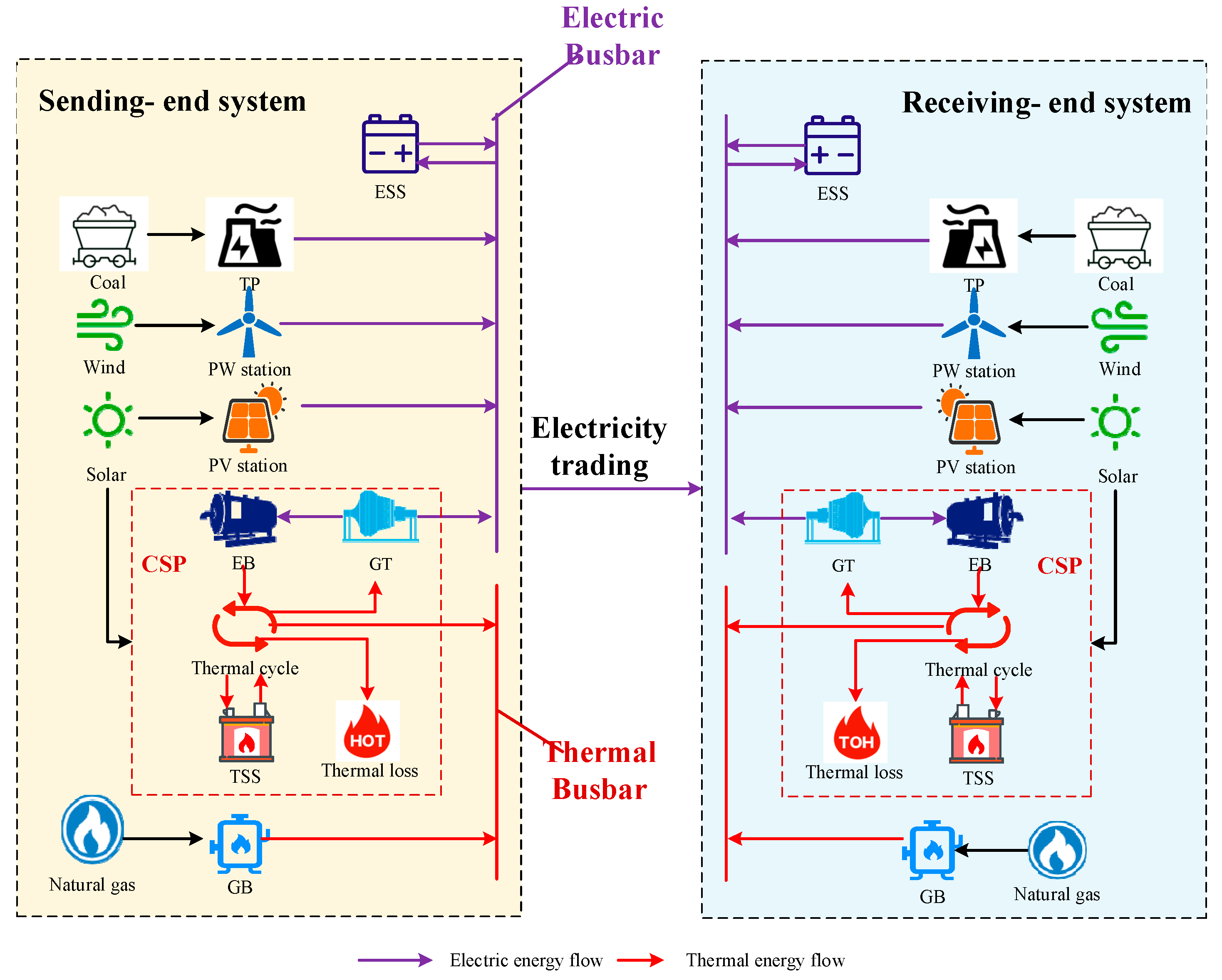
2. Cross-Area Interconnection System Model

Sending-End Power System

In an environment with a high proportion of renewable energy at the sending and receiving end, the wind-photo-thermal-fire co-generation system is constructed as shown in Figure 1. The system consists of the wind turbine (WT), photovoltaic (PV), gas turbine (GT), gas boiler (GB), electric boiler (EB), thermal power unit (TP), electric storage system (ESS), thermal storage system (TSS), and other equipment.

When wind power is significant, the electric heating device can convert part of the surplus wind power energy into heat energy stored in the heat storage link. In the peak load period, the heat energy stored in the heat storage link can be converted into electricity to increase the power generation of the CSP plant, which promotes the consumption of wind power and completes the energy time shift at the same time. The energy time-shift characteristics of the wind-photothermal joint complementary effect and the addition of thermal power units will further enhance the stability of the system operation to ensure the delivery of power adequacy. In addition to supplying power to the loads at the sending end, the surplus power is transmitted to the receiving end through the DC contact line.

The receiving system is fed power by DC tie lines and local thermal power units to meet the load demand. The structure of the receiving system is the same as that of the sending system and will not be described again here.

The delivery-end system is centred on a CSP plant equipped with an electric heating device. The CSP plant consists of three parts: heat collection, power generation, and storage. The thermal collector converts solar energy into thermal energy and then uses the thermal conductive mass to transmit the thermal energy. The transmitted thermal energy is converted into electric energy through the power generation link, completing the conversion of light-heat-electricity. In the heat storage link, the thermal conductive mass can carry out a two-way flow of energy, and its stored thermal energy can be used for power generation at any time.

The thermal energy collected in the heat collection link of the CSP plant can be expressed as:

$$P_{\mathrm{CSP},t}^{\mathrm{h}}={\eta }_{\mathrm{sh}}{S}_{\mathrm{CSP}}{I}_{s,t}$$

(1)

The formula for the electrical energy output of the CSP plant is as follows:

$$P_{\mathrm{CSP},t}^{\mathrm{e}}={\eta }_{\mathrm{he}}{P}_{\mathrm{CSP},t}^{\mathrm{he}}$$

(2)

The thermal storage model for the CSP plant is as follows:

$$Q_{\mathrm{TSS},t}=(1-{\epsilon }_{\mathrm{TSS}})Q_{\mathrm{TSS},t-1}+{\eta }_{\mathrm{TSS}}^{\mathrm{c}}{P}_{\mathrm{TSS},t}^{\mathrm{h},\mathrm{c}}\Delta t-\frac{P_{\mathrm{TSS},t}^{\mathrm{h},\mathrm{d}}}{{\eta }_{\mathrm{TSS}}^{\mathrm{d}}}\Delta t$$

(3)

The internal thermal cycle of the CSP plant satisfies:

$$P_{\mathrm{C}\mathrm{S}\mathrm{P},t}^{\mathrm{h}}+P_{\mathrm{E}\mathrm{B},t}^{\mathrm{h}}+P_{\mathrm{T}\mathrm{S}\mathrm{S},t}^{\mathrm{h},\mathrm{d}}=P_{\mathrm{T}\mathrm{S}\mathrm{S},t}^{\mathrm{h},\mathrm{c}}+P_{\mathrm{C}\mathrm{S}\mathrm{P},\mathrm{loss},t}^{\mathrm{h}}+P_{\mathrm{C}\mathrm{S}\mathrm{P},t}^{\mathrm{h}\mathrm{e}}$$

(4)

where $P_{\mathrm{CSP},t}^{\mathrm{e}}$ represents the power generated by the CSP plant; $P_{\mathrm{CSP},t}^{\mathrm{h}}$ is the thermal energy collected by the light field collector at time t; ${\eta }_{\mathrm{sh}}$ is the photothermal conversion efficiency of the CSP plant; $S_{\mathrm{CSP}}$ is the effective area of the light-field concentrating mirror; $I_{s,t}$ is the light intensity at the time; ${\eta }_{\mathrm{he}}$ is the efficiency of the conversion of thermal energy to electrical energy in the CSP plant; $P_{\mathrm{CSP},t}^{\mathrm{he}}$ is the thermal energy consumed by the CSP plant to drive the turbine to generate electricity at time t; $Q_{\mathrm{TSS},t}$, $Q_{\mathrm{TSS},t-1}$ are the heat storage capacity of the TSS at time t, t − 1, respectively; ${\epsilon }_{\mathrm{TSS}}$ is the rate of self-loss of heat from the TSS; ${\eta }_{\mathrm{TSS}}^{\mathrm{c}}$, ${\eta }_{\mathrm{TSS}}^{\mathrm{d}}$ are the heat storage and heat release efficiencies of the TSS, respectively; $P_{\mathrm{TSS},t}^{\mathrm{h},\mathrm{c}}$, $P_{\mathrm{TSS},t}^{\mathrm{h},\mathrm{d}}$ are the heat storage and exothermic power of the TSS at time t, respectively; $P_{\mathrm{CSP},\mathrm{loss},t}^{\mathrm{h}}$ is the heat loss of the CSP plant; $P_{\mathrm{EB},t}^{\mathrm{h}}$ is the heat energy produced by the EB at time t.

3. Economic Dispatch Model of a Cross-Regional Interconnected System

3.1. Objective Function

A source-grid-load cross-area coordinated optimization model based on IGDT and a wind-photovoltaic-photothermal system is proposed to achieve the lowest total system operation cost. The objective functions of the sending and receiving systems are the same. The optimization goal of the system operation can be formulated as follows:

$$\{\begin{array}{l}\min F=F_{\mathrm{om}}+F_{\mathrm{trade}}\\ F_{\mathrm{om}}={\displaystyle \sum _{t=1}^T{\lambda }_{y,\mathrm{om}}{P}_{y,t}}\\ F_{\mathrm{buy}}={\displaystyle \sum _{t=1}^T{\lambda }_{\mathrm{buy},t}^{\mathrm{e}}}{P}_{\mathrm{buy},t}^{\mathrm{e}}-{\displaystyle \sum _{t=1}^T{\lambda }_{\mathrm{sell},t}^{\mathrm{e}}}{P}_{\mathrm{sell},t}^{\mathrm{e}}\end{array}$$

(5)

where $F_{\mathrm{om}}$ and $F_{\mathrm{trade}}$ are the unit operation and maintenance cost and the electricity transaction cost, respectively; ${\lambda }_{y,\mathrm{om}}$ is the operation and maintenance cost coefficient of unit y; ${\lambda }_{\mathrm{buy},t}^{\mathrm{e}}$ and ${\lambda }_{\mathrm{sell},t}^{\mathrm{e}}$ are the power purchase price at time t, respectively; and $P_{\mathrm{buy},t}^{\mathrm{e}}$/$P_{\mathrm{sell},t}^{\mathrm{e}}$ is the purchased/sold electricity from the primary grid.

3.2. Constraints

(1)

Sending-end system constraints

(a)

Energy balance constraints

$$\{\begin{array}{l}{\mu }_{\mathrm{GB}}^{\mathrm{e}}{P}_{\mathrm{GB},t}^{\mathrm{e}}+P_{\mathrm{g},t}^{\mathrm{e}}+P_{\mathrm{buy},t}^{\mathrm{e}}+P_{\mathrm{v},t}^{\mathrm{e}}+P_{\mathrm{w},t}^{\mathrm{e}}+\\ P_{\mathrm{CSP},t}^{\mathrm{e}}+P_{ESS,t}^{\mathrm{d}}=L_t^{\mathrm{e}}+P_{\mathrm{sell},t}^{\mathrm{e}}+P_{ESS,t}^{\mathrm{c}}+P_{\mathrm{EB},t}^{\mathrm{h}}/{\eta }_{\mathrm{EB},t}^{\mathrm{h}}\\ {\mu }_{\mathrm{GB}}^{\mathrm{h}}{P}_{\mathrm{GB},t}^{\mathrm{h}}+P_{\mathrm{CSP},t}^{\mathrm{h}}=L_t^{\mathrm{h}}\end{array}$$

(6)

where $P_{\mathrm{GB},t}^{\mathrm{e}}$, $P_{\mathrm{g},t}^{\mathrm{e}}$, $P_{\mathrm{w},t}^{\mathrm{e}}$, $P_{\mathrm{v},t}^{\mathrm{e}}$, and $P_{\mathrm{CSP},t}^{\mathrm{e}}$ represent the electric power output of the GB, TP, WT, PV and CSP plant at time t, respectively; $P_{\mathrm{GB},t}^{\mathrm{h}}$, $P_{\mathrm{EB},t}^{\mathrm{h}}$ and $P_{\mathrm{CSP},t}^{\mathrm{h}}$ represent the heating power output of the GB, EB and CSP plant at time t, respectively; and ${\eta }_{\mathrm{EB},t}^{\mathrm{h}}$ is the EB’s electrical heat transfer coefficient.

(b)

The upper and lower output constraints of other units

$$\{\begin{array}{l}0< P_{\mathrm{w},t}^{\mathrm{e}}< P_{\mathrm{w},t}^{\mathrm{pre}}\\ 0< P_{\mathrm{v},t}^{\mathrm{e}}< P_{\mathrm{v},t}^{\mathrm{pre}}\\ P_{\mathrm{GB},\min }^{\mathrm{e}}\le P_{\mathrm{GB},t}^{\mathrm{e}}\le P_{\mathrm{GB},\max }^{\mathrm{e}}\\ P_{\mathrm{g},\min }^{\mathrm{e}}\le P_{\mathrm{g},t}^{\mathrm{e}}\le P_{\mathrm{g},\max }^{\mathrm{e}}\\ P_{\mathrm{CSP},\min }^{\mathrm{e}}\le P_{\mathrm{CSP},t}^{\mathrm{e}}\le P_{\mathrm{CSP},\max }^{\mathrm{e}}\\ P_{\mathrm{CSP},\min }^{\mathrm{h}}\le P_{\mathrm{CSP},t}^{\mathrm{h}}\le P_{\mathrm{CSP},\max }^{\mathrm{h}}\\ P_{\mathrm{GB},\min }^{\mathrm{h}}\le P_{\mathrm{GB},t}^{\mathrm{h}}\le P_{\mathrm{GB},\max }^{\mathrm{h}}\\ P_{\mathrm{EB},\min }^{\mathrm{h}}\le P_{\mathrm{EB},t}^{\mathrm{h}}\le P_{\mathrm{EB},\max }^{\mathrm{h}}\\ P_{\mathrm{buy},\min }^{\mathrm{e}}\le P_{\mathrm{buy},t}^{\mathrm{e}}\le P_{\mathrm{buy},\max }^{\mathrm{e}}\\ P_{\mathrm{sell},\min }^{\mathrm{e}}\le P_{\mathrm{sell},t}^{\mathrm{e}}\le P_{\mathrm{sell},\max }^{\mathrm{e}}\end{array}$$

(7)

where $P_{\mathrm{w},t}^{\mathrm{pre}}$ and $P_{\mathrm{v},t}^{\mathrm{pre}}$ are the predicted output of WT and PV, respectively; $P_{\mathrm{GB},\max }^{\mathrm{e}}$, $P_{\mathrm{buy},\max }^{\mathrm{e}}$, $P_{\mathrm{g},\max }^{\mathrm{e}}$, $P_{\mathrm{CSP},\max }^{\mathrm{e}}$ and $P_{\mathrm{sell},\max }^{\mathrm{e}}$ represent the maximum electric power of the GB, purchased electricity, TP, CSP plant, and sold electricity respectively; $P_{\mathrm{GB},\max }^{\mathrm{h}}$, $P_{\mathrm{EB},\max }^{\mathrm{h}}$, and $P_{\mathrm{CSP},\max }^{\mathrm{h}}$ represent the full electric power of GB, EB and CSP plant respectively; $P_{\mathrm{GB},\min }^{\mathrm{e}}$, $P_{\mathrm{buy},\min }^{\mathrm{e}}$, $P_{\mathrm{g},\min }^e$, $P_{\mathrm{CSP},\min }^{\mathrm{e}}$ and $P_{\mathrm{sell},\min }^{\mathrm{e}}$ represent the minimum heat power of the GB, purchased electricity, TP, CSP plant, and sold electricity respectively; and $P_{\mathrm{GB},\min }^{\mathrm{h}}$, $P_{\mathrm{EB},\min }^{\mathrm{h}}$, and $P_{\mathrm{CSP},\min }^{\mathrm{h}}$ represent the minimum heat power of GB, EB and CSP plant respectively.

(c)

Energy storage device constraints

This paper uses generalized energy storage modelling for the electric storage and thermal storage of the CSP plant. The energy storage charge state and power constraints are as follows:

$$\{\begin{array}{l}{Q}_{s,t}=Q_{s,t-1}(1-{\epsilon }_s)+P_{s,t}^{\mathrm{c}}{\eta }_s^{\mathrm{c}}{u}_{s,t}^{\mathrm{c}}\Delta t-\frac{P_{s,t}^{\mathrm{d}}{u}_{s,t}^{\mathrm{d}}\Delta t}{{\eta }_s^d}\\ Q_{\mathrm{s},\min }\le Q_{s,t}\le Q_{s,\max }\end{array}$$

(8)

$$\{\begin{array}{l}0\le u_{s,t}^{\mathrm{c}}+u_{s,t}^{\mathrm{d}}\le 1\\ u_{s,t}^{\mathrm{c}}{P}_{s,\min }^{\mathrm{c}}\le P_{s,t}^{\mathrm{c}}\le u_{s,t}^{\mathrm{c}}{P}_{s,\max }^{\mathrm{c}}\\ u_{s,t}^{\mathrm{d}}{P}_{s,min}^{\mathrm{d}}\le P_{s,t}^{\mathrm{d}}\le u_{s,t}^{\mathrm{d}}{P}_{s,max}^{\mathrm{d}}\\ {\displaystyle \sum _{t=1}^{\mathrm{T}}{P}_{s,t}^{\mathrm{c}}{\eta }_s^{\mathrm{c}}}\Delta t={\displaystyle \sum _{t=1}^{\mathrm{T}}\frac{P_{s,t}^{\mathrm{d}}\Delta t}{{\eta }_s^{\mathrm{d}}}}\end{array}$$

(9)

where s represents the type of energy storage devices; s = 1, 2 represents ESS and TSS, respectively; $u_{s,t}^{\mathrm{c}}$ and $u_{s,t}^{\mathrm{d}}$ are binary variables, which refer to the charging and discharging state parameters of the energy storage device s at time t, respectively; $Q_{s,t}$ is the capacity of the energy storage device s at time t; ${\epsilon }_s$ is the self-discharge rate of energy storage device s; ${\eta }_s^{\mathrm{c}}$ and ${\eta }_s^{\mathrm{d}}$ are the charging and discharging power of energy storage device s, respectively; $Q_{s,\max }$ and $Q_{s,\min }$ are the charging and discharging power of energy storage device s, respectively; $P_{s,\min }^{\mathrm{c}}$ and $P_{s,\max }^{\mathrm{c}}$ are the maximum and minimum charging power of energy storage device s, respectively; and $P_{s,\min }^{\mathrm{d}}$ and $P_{s,\max }^{\mathrm{d}}$ are the maximum and minimum discharging power of energy storage device s, respectively.

• (d)

  Network security constraints

  $$-L_{l,\max }\le L_{l,t}={\displaystyle \sum _{n=1}^{\mathrm{N}}{G}_{l,n}{P}_{t,n}}\le L_{l,\max }$$

  (10)

  where $L_{l,t}$ is the DC power flow of the power system at time t; $L_{l,\max }$ is the maximum transmission capacity of line l; $G_{l,n}$ is the transfer distribution factor of node n to line l; $P_{t,n}$ is the active power injection power of node n at time t; and N is the total number of nodes.

(2)

Receiving-end system constraints

The receiving-end system’s balancing restrictions, unit output constraints, energy storage constraints, and cybersecurity constraints are all identical to those of the sending-end system. The limitations on the receiving-end system are not stated here.

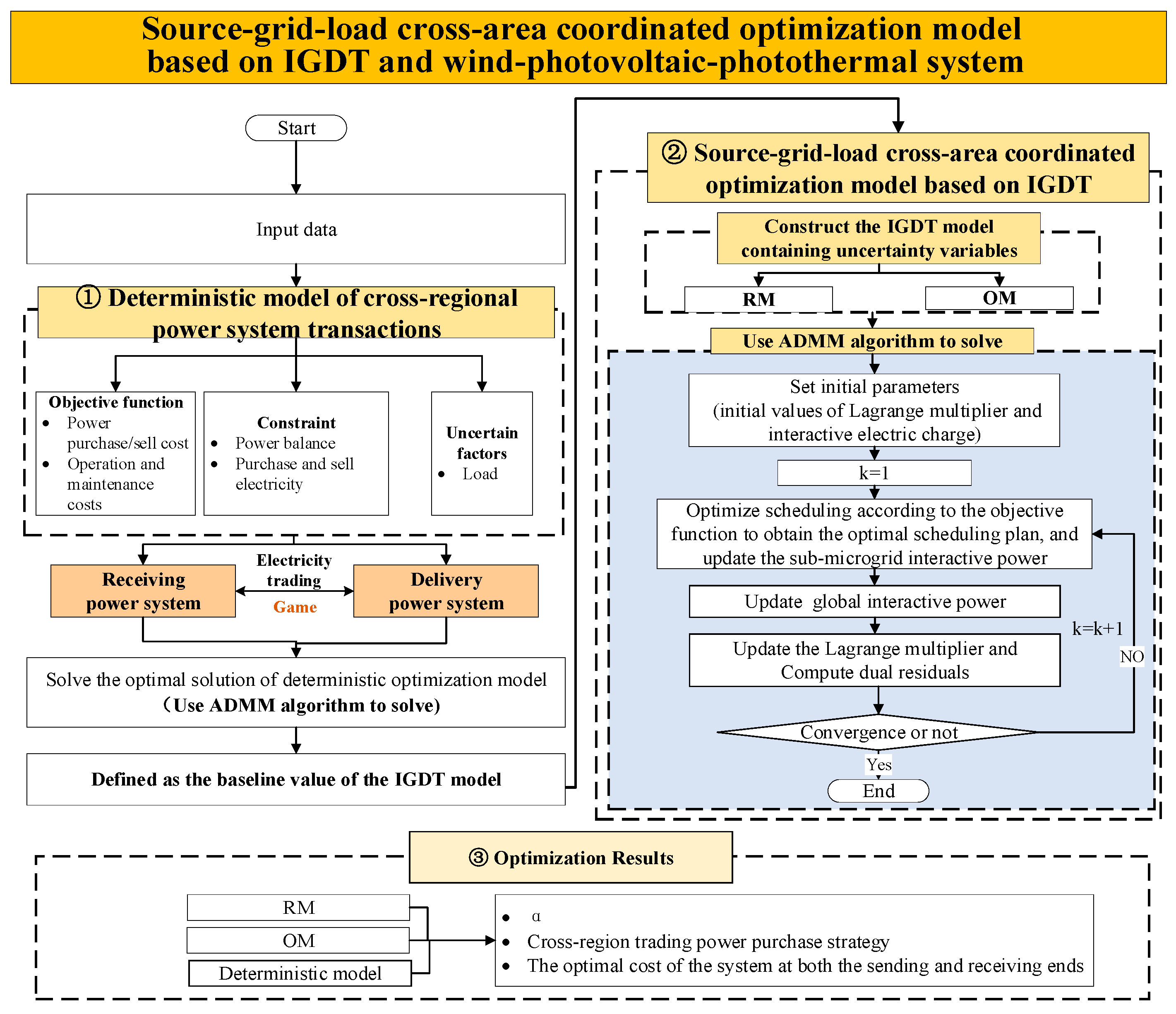
3.3. Optimization Model Based on IGDT

Information gap decision theory (IGDT) is an optimization technique that may successfully deal with system uncertainties. In this sense, information refers to data that introduce uncertainty into a system and impact the system’s aim. The gap is the difference between the projected and actual values of the uncertainty. When the system’s uncertain parameters are difficult to define in terms of probability, the information gap model can be used. The uncertainty parameter, x, is expressed as follows:

$$\{\begin{array}{l}x\in U(\alpha ,x^{*})\\ U(\alpha ,x^{*})=\left\{x:\left|\frac{x-x^{*}}{x^{*}}\right|⩽\alpha \right\}\end{array}$$

(11)

where $x^{*}$ is the predicted value of $x$; $\alpha$ represents the uncertainty radius of the parameter and $\alpha$ ≥ 0; and $U$ represents the fluctuation range of the parameter. The maximum fluctuation range of $x^{*}$ is $\pm \alpha x^{*}$.

The scheduling models for the sending- and receiving-end systems are the same. Based on the IGDT theory, the model is reconstructed using the delivery-end system as an example:

$$\{\begin{array}{l}\min F(x,v)\hfill \\ \mathrm{s}.\mathrm{t}. H(x,v)=0\hfill \\ G(x,v)⩽0\hfill \end{array}$$

(12)

where $F$ is the objective function; $v$ represents the decision variable; $H(x,v)$ is the model equation constraint; and $G(x,v)$ is the model inequality constraint.

In this paper, the uncertainty in electrical and thermal loads is modelled using envelope constraints. The expressions are as follows:

$$\{\begin{array}{l}{L}_t^{\mathrm{e}}\in U({\alpha }^{\mathrm{L}},L_t^{\mathrm{e}*}),0⩽{\alpha }^{\mathrm{L}}\\ L_t^{\mathrm{h}}\in U({\alpha }^{\mathrm{L}},L_t^{\mathrm{h}*}),0⩽{\alpha }^{\mathrm{L}}\\ U({\alpha }^{\mathrm{L}},L_t^{\mathrm{e}*})=\left\{L_t^{\mathrm{e}}:\left|\frac{L_t^{\mathrm{e}}-L_t^{\mathrm{e}*}}{L_t^{\mathrm{e}*}}\right|⩽{\alpha }^{\mathrm{L}}\right\}\\ U({\alpha }^{\mathrm{L}},L_t^{\mathrm{h}*})=\left\{L_t^{\mathrm{h}}:\left|\frac{L_t^{\mathrm{h}}-L_t^{\mathrm{h}*}}{L_t^{\mathrm{h}*}}\right|⩽{\alpha }^{\mathrm{L}}\right\}\end{array}$$

(13)

where ${\alpha }^{\mathrm{L}}$ is the uncertainty of the load, i.e., the gap between the actual and predicted values of the load. The maximum variations between the real and anticipated values of the electric and thermal loads are denoted by the letters $\pm {\alpha }^{\mathrm{L}}{L}_t^{\mathrm{e}*}$ and $\pm {\alpha }^{\mathrm{L}}{L}_t^{\mathrm{h}*}$.

Based on the decision maker’s risk bias, the following expressions are used to build an opportunity model (OM) and a robustness model (RM):

$$\{\begin{array}{l}\min {\alpha }^{\mathrm{L}}\\ s.t.\min F(L_t^{\mathrm{e}*},L_t^{\mathrm{h}*},v)\le (1-{\beta }^{\mathrm{OM}})F_0\\ \forall x\in U({\alpha }^{\mathrm{L}},L_t^{\mathrm{e}*},L_t^{\mathrm{h}*})\\ \mathrm{Equation} (1)-\mathrm{Equation} (10)\end{array}$$

(14)

$$\{\begin{array}{l}\max {\alpha }^{\mathrm{L}}\\ s.t.\max F(L_t^{\mathrm{e}*},L_t^{\mathrm{h}*},v)\le (1+{\beta }^{\mathrm{RM}})F_0\\ \forall x\in U({\alpha }^{\mathrm{L}},L_t^{\mathrm{e}*},L_t^{\mathrm{h}*})\\ \mathrm{Equation} (1)-\mathrm{Equation} (10)\end{array}$$

(15)

Equation (14) is the OM, which transforms the deterministic model’s optimization objective Equation (8) into a minimum uncertainty radius, ${\alpha }^{\mathrm{L}}$, that meets the target cost of less than $(1-{\beta }^{\mathrm{OM}})F_0$. The smaller the ${\alpha }^{\mathrm{L}}$ obtained by the OM, the more likely the corresponding decision scheme will have a positive result.

Equation (15) is the RM. The RM transforms the optimization objective of the deterministic model Equation (8) into finding the maximum uncertainty radius ${\alpha }^{\mathrm{L}}$ that satisfies the target cost no larger than $(1+{\beta }^{\mathrm{OM}})F_0$. The bigger ${\alpha }^{\mathrm{L}}$ obtained by the RM shows that the model is less susceptible to parameter uncertainty, i.e., the better the resilience is. ${\beta }^{\mathrm{RM}}$ and ${\beta }^{\mathrm{OM}}$ are cost deviation factors created by the decision maker to indicate the level of permissible deviation of the predicted cost above or below the benchmark value, respectively.

3.4. Model Solution

In this paper, the ADMM algorithm is used to solve the problem. The advantage of the ADMM algorithm is that it can make full use of the decomposability of the objective function, and then alternately optimize the multivariate variables in the objective function to improve the feasibility of the solution. The ADMM algorithm consists of the original residuals and the dyadic residuals as the two convergence parameters. When the actual residuals and the pairwise residuals of the transaction volume of the sending system and the receiving system satisfy the convergence accuracy, the model exits the iteration and obtains the optimal solution. The computational principle of the ADMM algorithm is described in the literature [15] and will not be repeated in this paper.

Considering the system’s preference for risk, this paper constructs an IGDT-based inter-area dispatch model of a power system to balance the economy and stability of the two systems. The model solution process is shown in Figure 2.

4. Example Analysis

4.1. Input Data and Scenario Setup

(1)

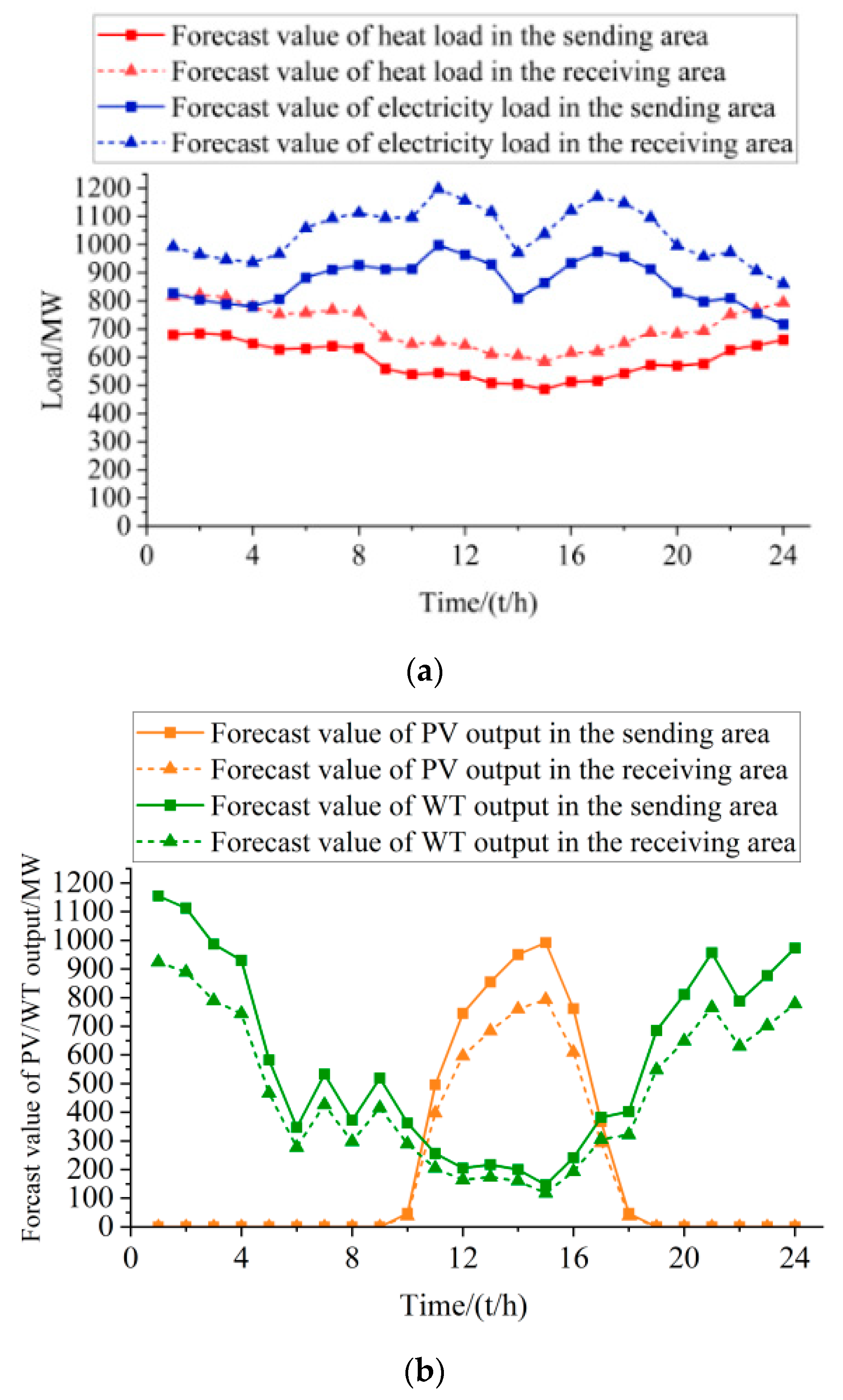
Input data

This example is based on the power grid development plan of a region. According to the planning data, each region’s installed capacity and installed share are as shown in

Table 1. Power supply installation data of the sending end system.

Installation	Capacity	Proportion
Wind Power	1200	23.24%
Photovoltaic	900	17.43%
Photothermal	1800	34.86%
Thermal Power	1163	22.53%
Gas boilers	100	1.94%
Final Assembly Machine	5163	100.00%

. The day-ahead forecast values of WT and PV output and load for a typical day are as shown in Figure 3.

(2)

Scenario setup

Three scenarios were investigated to analyze the optimization effect of the proposed system scheduling model. The scenario details are listed in

Table 2. Scenario classification.

Scenario	1	2	3
CSP plant	√	√	√
IGDT (risk-seeking strategy)	×	√	√
IGDT (risk-averse strategy)	×	×	√

.

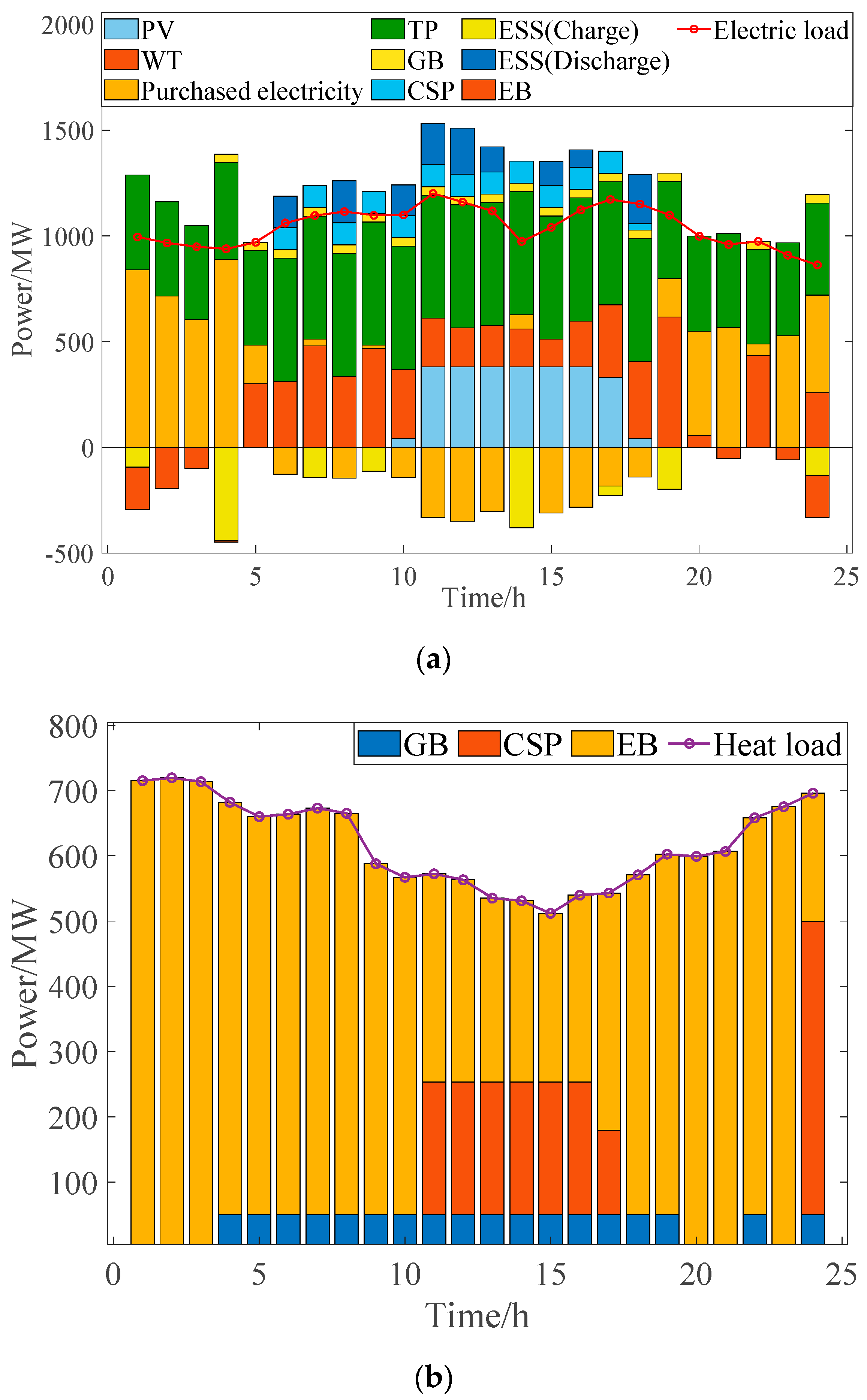
4.2. Operation Analysis

(1)

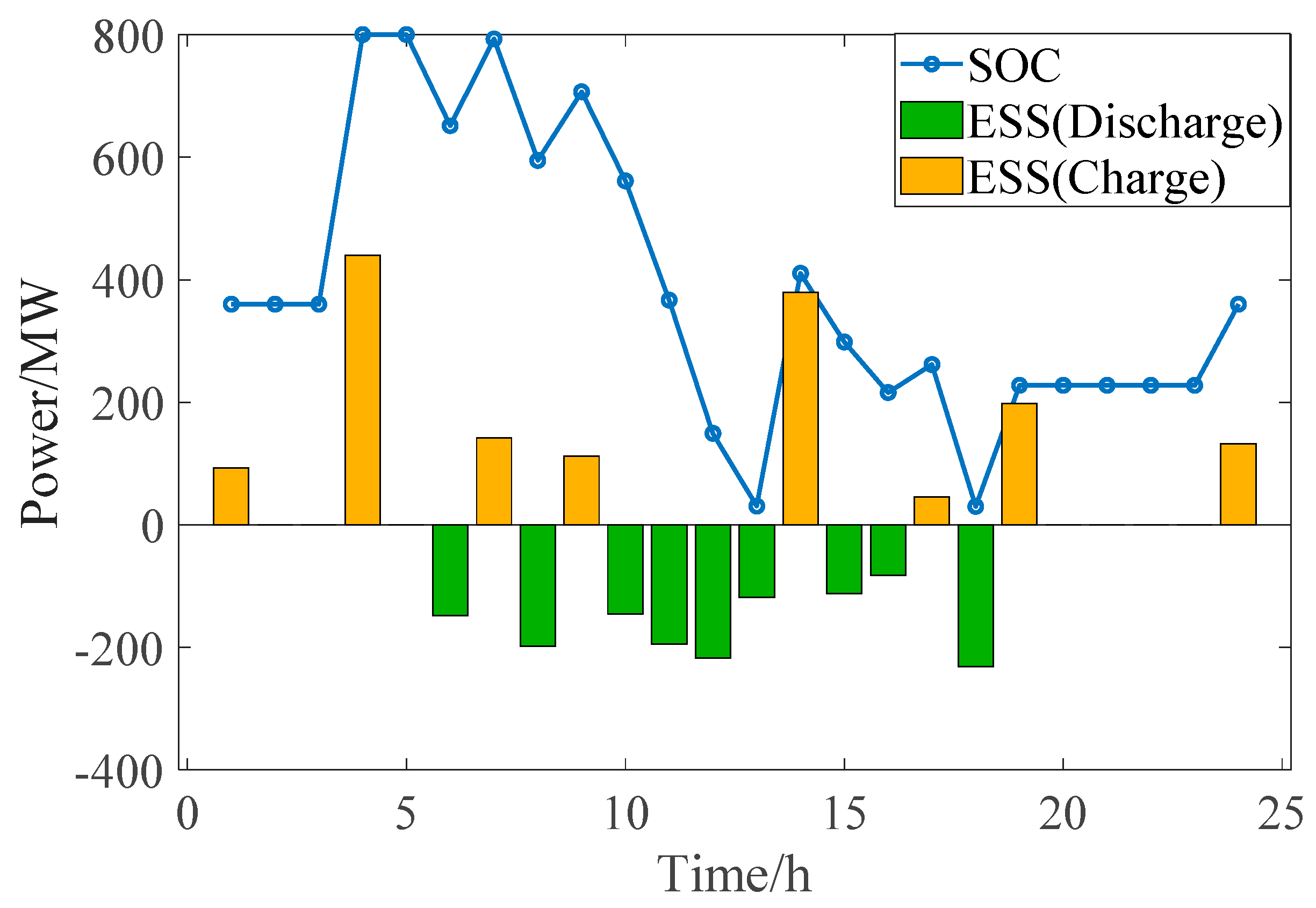
Scheduling results

The amount of electricity traded, the total dispatch cost of the receiving system, and the total dispatch cost of the sending system for the three scenarios are shown in

Table 3. Optimization results of the power system in 3 scenarios.

Scenario	Scenario 1	Scenario 2	Scenario 3
Electricity Trading Volume/MW	2875.44	2114.40	1304.11
Sending-end system cost/CNY	28,766	17,690	32,854
Receiving-end system cost/CNY	128,662	81,030	72,297

.

The load demand is determined under Scenario 1, and the CSP plant is introduced into both the sending and receiving systems to enhance the utilization of light energy. Using the receiving system as an example, Figure 4 depicts the scheduling result of the CSP plant. During the 11:00–17:00 time period, when the light is intense, the CSP plant transforms the extra light into heat and stores it in the thermal storage system, increasing the system’s energy efficiency. The receiving system has acquired 2875.44 MW of power from the transmitting system. The receiving system has a high power buy cost due to the purchased power, costing 128,662 CNY.

Compared to Scenario 1, Scenario 2 employs the information gap decision theory to assess load uncertainty. Scenario 2 uses the opportunity pursuit method, and the system can handle multi-source collaborative scheduling under certain conditions. In Scenario 2, the power purchased by the receiving system fell by 36.00%. The load curve shifted after the model added IGDT to measure the uncertainty of electric and heating loads. To minimize the total cost of the receiving system, the power purchased was reduced, resulting in a 58.78% cost reduction. Although the delivery system’s energy sales revenue has declined, unit operation and maintenance costs have decreased due to low load during specific periods. Thus, the OM improves the economics of both the sending and receiving systems.

In Scenario 3, the system at both the sending and receiving ends is willing to sacrifice part of the system’s economy when load fluctuations are severe and to adjust the unit’s output to ensure system stability. The ADMM technique is used in this paper to solve the problem efficiently. The model finishes the iteration for the 32nd time, and the iteration curve is illustrated in Figure 5.

Under the risk-averse strategy, the sending system adjusts the output of specific units to maintain electric and thermal balance and minimize the impact of load fluctuation on the system. In this scenario, the cost of the sending system experiences an increase of 85.72% while the system becomes more resilient. The receiving system unit can satisfy the load demand with its output. Figure 6 displays the outcomes of the load balance analysis for both the electric and thermal aspects of the receiving system. The gas boiler units, WT, PV, and the CSP plant all have positive power. Co-dispatching the different types of units maximizes their outputs to meet the heat and electricity demand of the system while minimizing the overall cost of the system. Simultaneously, the thermal and electric energy storage tanks accomplish a transfer of power in both space and time, thereby increasing the efficiency of energy use.

Figure 7 shows the charging and discharging outcomes of the energy storage in the receiving-end system. Energy storage undergoes charging during periods of low demand and discharging during periods of high demand, thereby minimizing the disparity between peak and low load levels. Furthermore, to enhance the system’s economy, the receiving system implemented a further reduction in the quantity of electric energy procured, resulting in a 12.08% decrease in system cost. Consequently, implementing the RM improves the sending system’s resilience and enhances the receiving system’s efficiency.

The amount of electricity traded at each moment under the three scenarios is shown in Figure 8. Under the deterministic model, the amount of power purchased by the end-system is more significant than that in Scenario 2 and Scenario 3 for the periods 0:00–8:00 and 22:00–24:00, which indicates that the load of the system is reduced in these two time periods after the model applies the IGDT to measure load uncertainty, and the end system does not have to bear the high cost of purchasing power. Except for 10:00–12:00, the purchased power of the recipient system in Scenario 2 is more significant than that in Scenario 3. Under the risk-averse strategy, the recipient system reduces the amount of energy traded. It increases the output of various types of units to balance the economy and stability of the system.

(2)

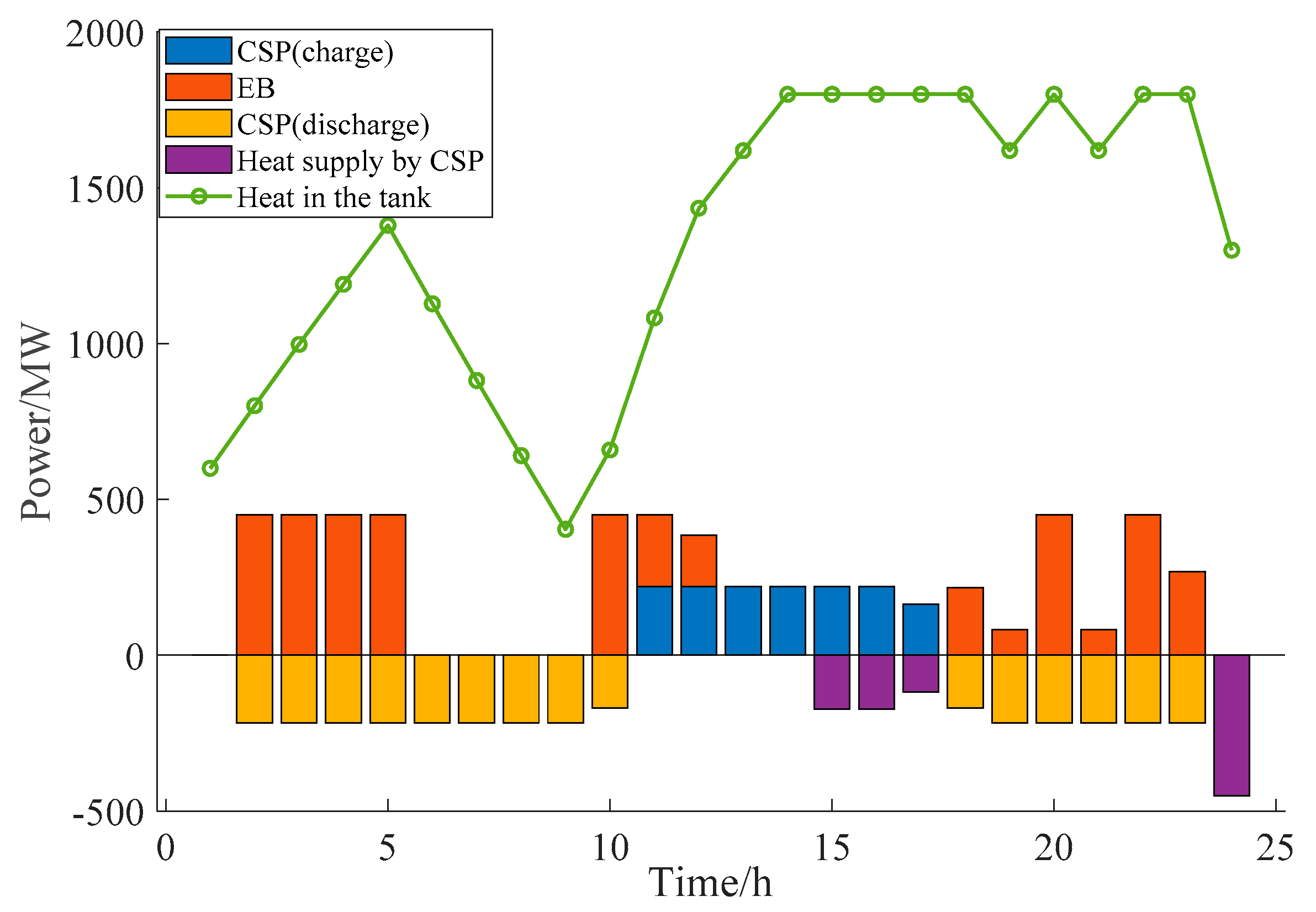
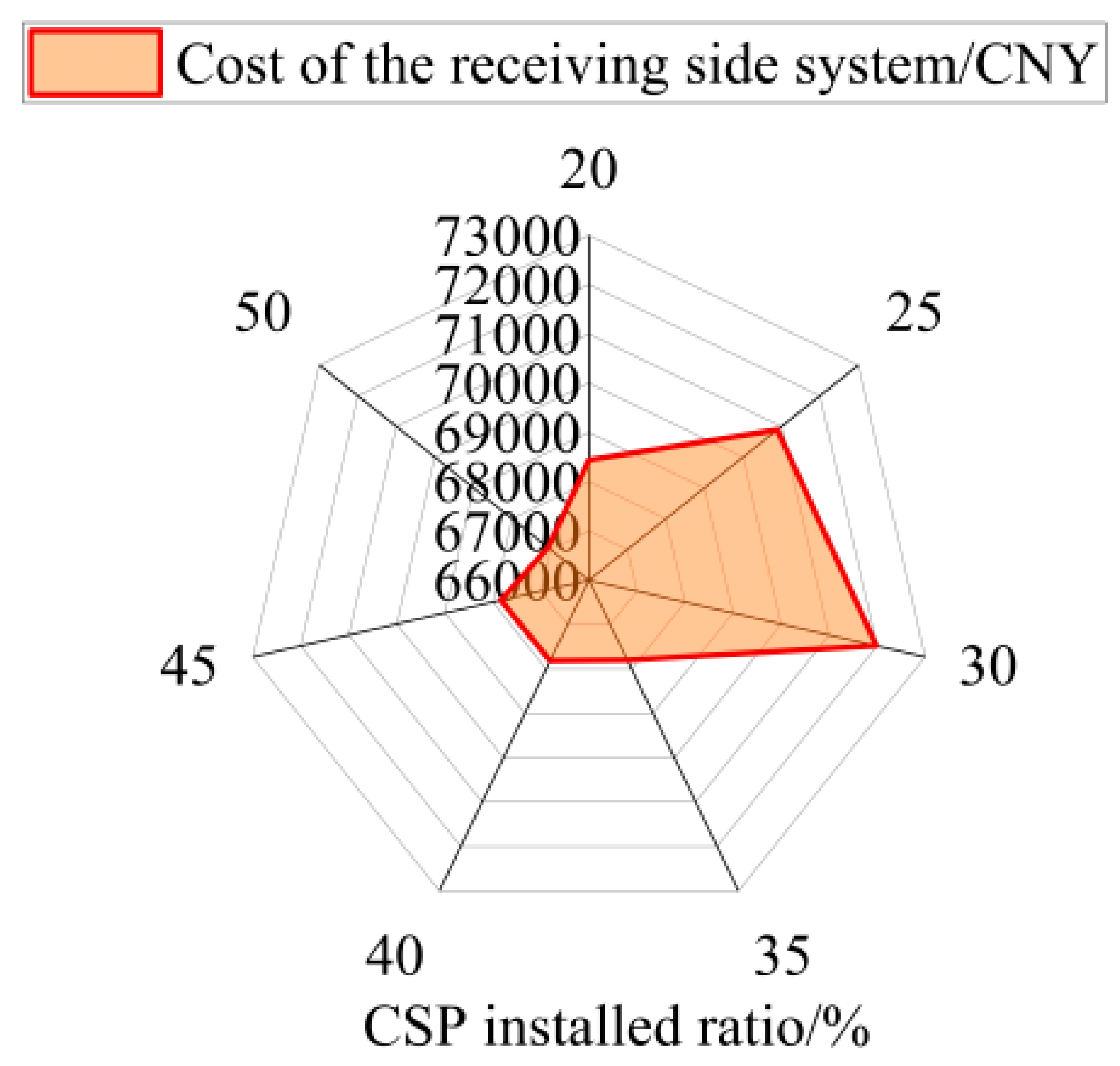
Analysis of CSP plants’ capacity

The proportion of PV access to the grid will further expand in the future, and the system cost will fluctuate with the change in the installed proportion of the CSP plant, which affects the system peaking effect. Assuming that the regulating capacity of the unit remains unchanged, Scenario 3 is used as the base scenario to explore the impact of the installed proportion of the CSP plant on the system cost of the recipient system. The total cost of the recipient system under different established proportions of the CSP plant is shown in Figure 9. When the installed proportion of the CSP plant is in the interval of [20%, 30%], the system’s total cost gradually increases with the increase in the installed proportion of the CSP plant. When the installed proportion of CSP plants is in the interval of (30%, 50%], the total cost of the system gradually decreases with the increase in the installed proportion of the CSP plant. The reason is that at the initial stage of CSP plant installation, the O&M cost of the CSP plant increases with the rise of its installed proportion, which leads to an increase in total system cost. When the proportion of the CSP plant is increased to more than 30%, the CSP plant can fully absorb excess light energy and maintain the system’s stability through photothermal conversion, which improves the rate of renewable energy consumption.

(3)

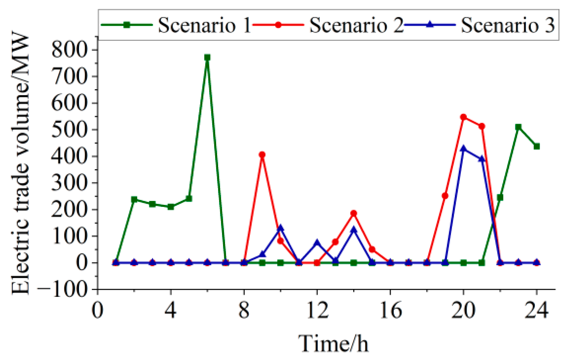
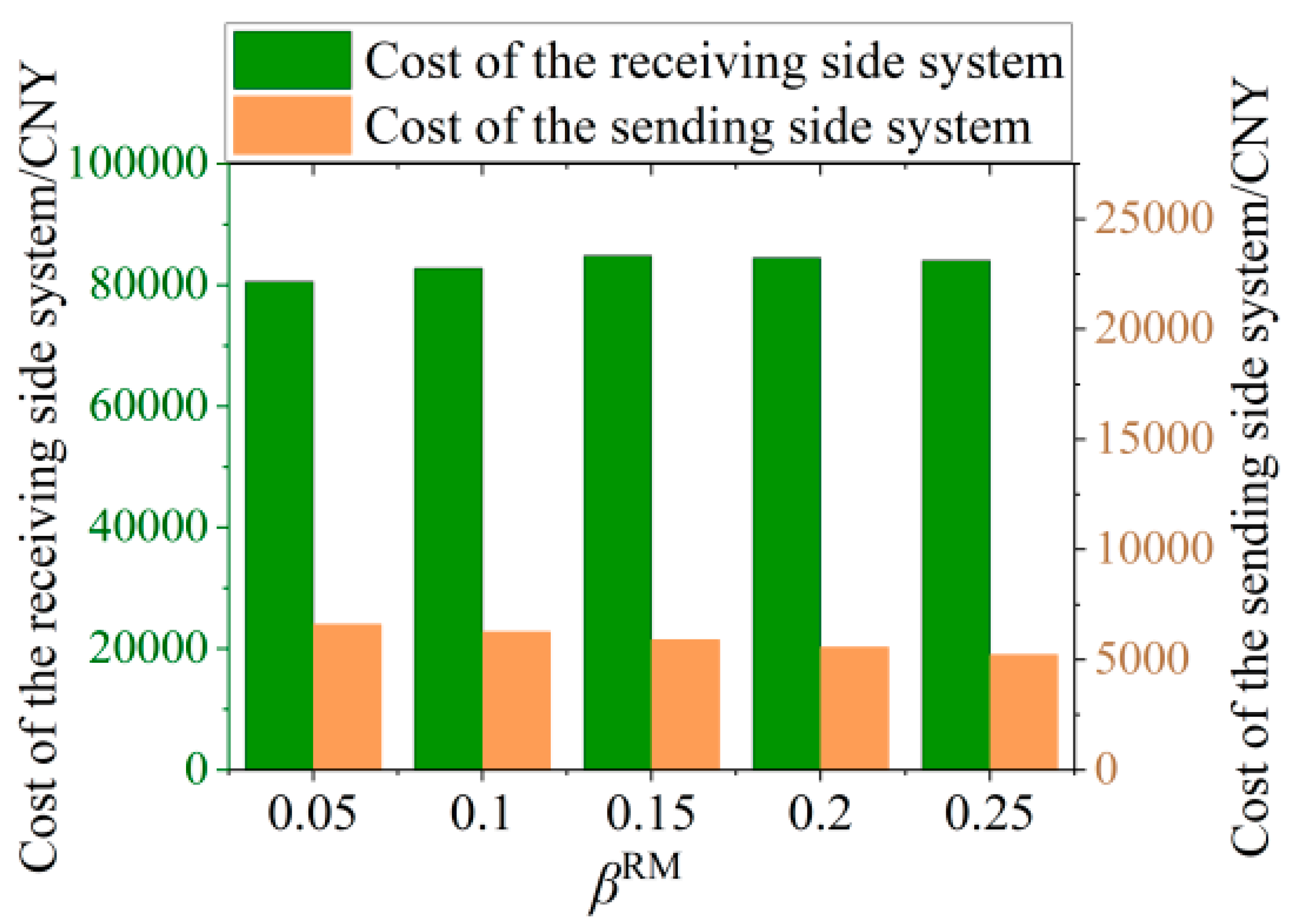
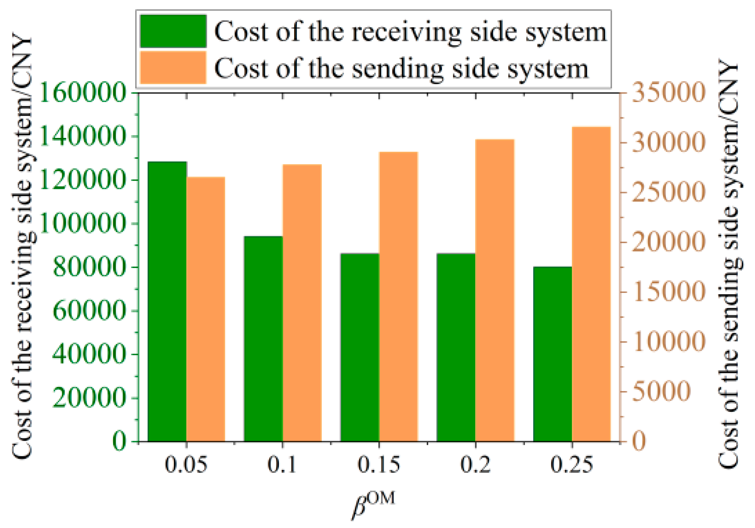
Impact of IGDT on scheduling results

This paper investigates the impact of electric and heating load uncertainty on the system. It provides decision-making solutions under various risk attitudes by varying the chance/robust deviation factor range. Figure 10 and Figure 11 show the change diagrams for total system scheduling costs under OM and RM, respectively. Figure 10 shows that under OM, as the deviation factor increases, the total cost of the receiving-end system decreases while the total cost of the sending-end system gradually increases. As a result, under the opportunity pursuit strategy, an increase in the deviation factor has a more significant positive impact on the economics of the receiving system.

Figure 11 shows that the RM’s sending- and receiving-end systems are relatively robust. As the deviation factor increases, the receiving system must purchase more power to maintain system stability, increasing the receiving system’s cost over time. The sending-end system benefits from electric energy trading, gradually reducing its cost. As a result, under the risk-averse strategy, an increase in the deviation factor improves the sending system’s economics.

5. Conclusions

In order to solve the new energy abandonment problem of the power system under large-scale wind and solar grid integration, this paper proposes a source-grid-load cross-area coordinated optimization method based on IGDT and a wind-photovoltaic-photothermal system, which reduces the impacts of the uncertainties of the source and load sides on the scheduling of the system at both the sending and receiving ends.

(1)

The source-grid-load coordinated scheduling can more reasonably formulate the scheduling plan according to the regulation period and regulation characteristics of the three sides of the peaking resources so as to effectively realize the coordination and complementarity of the peaking resources on each side. At the same time, the comprehensive operating cost of the system is reduced.

(2)

The introduction of information gap decision theory can reduce the impact of load uncertainty on the system scheduling results. Based on IGDT theory, this paper proposes a coordinated inter-area scheduling strategy for source-network-load of the wind-photovoltaic-photothermal system, including both risk-seeking and risk-averse strategies, which can provide decision-making references for the scheduling strategy makers.

(3)

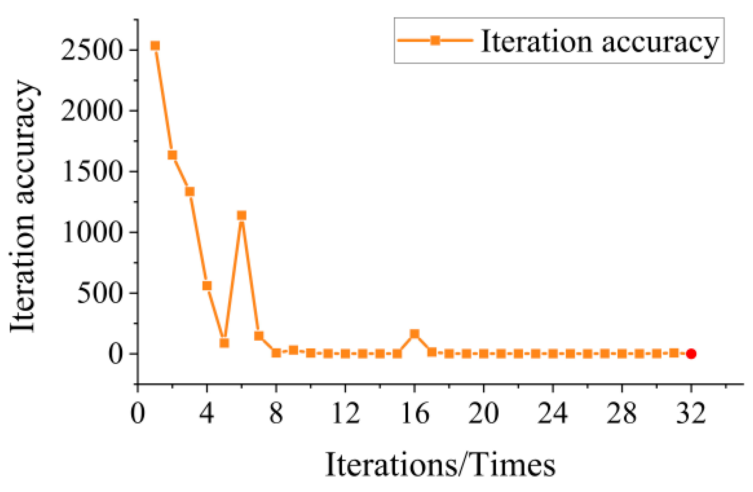
The ADMM algorithm is introduced into the solution of the cross-area power trading model, which can prevent the model from falling into the local optimal solution and improve the solution efficiency.

However, the IGDT model does have some limitations. First, the baseline value determines the validity of the IGDT model. Future research should investigate a more scientific method of establishing baseline values to improve the model’s effectiveness and rationality. Second, the IGDT model’s efficiency may be low when considering uncertainty fluctuations. Future research should compare and analyze the advantages and disadvantages of various algorithms and the solving efficiency to improve the accuracy of the IGDT model solution.

References

- Mang, L.; Chakrabortty, A. Optimization algorithms for catching data manipulators in power system estimation loops. IEEE Trans. Control Syst. Technol. 2018, 27, 1203–1218. [Google Scholar]
- Duan, L.; Lu, H.; Yuan, M.; Lv, Z. Optimization and part-load performance analysis of MCFC/ST hybrid power system. Energy 2018, 152, 682–693. [Google Scholar] [CrossRef]
- Darvish Falehi, A. Optimal robust disturbance observer based sliding mode controller using multi-objective grasshopper optimization algorithm to enhance power system stability. J. Ambient. Intell. Humaniz. Comput. 2020, 11, 5045–5063. [Google Scholar] [CrossRef]
- Okundamiya, M.S. Size optimization of a hybrid photovoltaic/fuel cell grid connected power system including hydrogen storage. Int. J. Hydrogen Energy 2020, 46, 30539–30546. [Google Scholar] [CrossRef]
- Pilotti, M.L.; Colombari, A.F.; Binotti, M.; Giaconia, A.; Martelli, E. Simultaneous design and operational optimization of hybrid CSP-PV plants. Appl. Energy 2023, 331, 120369. [Google Scholar] [CrossRef]
- Li, X.; Li, T.; Liu, L.; Wang, Z.; Li, X.; Huang, J.; Huang, J.; Guo, P.; Xiong, W. Operation optimization for integrated energy system based on hybrid CSP-CHP considering power-to-gas technology and carbon capture system. J. Clean. Prod. 2023, 391. [Google Scholar] [CrossRef]
- Yang, H.; Zhou, M.; Wu, Z.; Zhang, M.; Liu, S.; Guo, Z.; Du, E. Exploiting the operational flexibility of a concentrated solar power plant with hydrogen production. Sol. Energy 2022, 247, 158–170. [Google Scholar] [CrossRef]
- Gao, J.; Wu, H.; Gao, F. Nearly-zero carbon optimal operation model of hybrid renewable power stations comprising multiple energy storage systems using the improved CSO algorithm. J. Energy Storage 2024, 79, 110158. [Google Scholar] [CrossRef]
- Devarapalli, R.; Bhattacharyya, B. A hybrid modified grey wolf optimization-sine cosine algorithm-based power system stabilizer parameter tuning in a multimachine power system. Optim. Control Appl. Methods 2020, 41, 1143–1159. [Google Scholar] [CrossRef]
- Zhang, J.; Chen, Z.; He, C.; Jiang, Z.; Guan, L. Data-Driven-Based Optimization for Power System Var-Voltage Sequential Control. IEEE Trans. Ind. Inform. 2018, 15, 2136–2145. [Google Scholar] [CrossRef]
- Ruan, G.; Zhong, H.; Zhang, G.; He, Y.; Wang, X.; Pu, T. Review of learning-assisted power system optimization. CSEE J. Power Energy Syst. 2020, 7, 221–231. [Google Scholar]
- Srivastava, A.; Das, D.K. A new aggrandized class topper optimization algorithm to solve economic load dispatch problem in a power system. IEEE Trans. Cybern. 2020, 52, 4187–4197. [Google Scholar] [CrossRef]
- Alzahrani, A.; Sajjad, K.; Hafeez, G.; Murawwat, S.; Khan, S.; Khan, F.A. Real-time energy optimization and scheduling of buildings integrated with renewable microgrid. Appl. Energy 2023, 335, 120640. [Google Scholar] [CrossRef]
- Xu, X.; Hu, W.; Liu, W.; Du, Y.; Huang, Q.; Chen, Z. Robust energy management for an on-grid hybrid hydrogen refueling and battery swapping station based on renewable energy. J. Clean. Prod. 2021, 331, 129954. [Google Scholar] [CrossRef]
- Hu, J.; Wang, Y.; Dong, L. Low carbon-oriented planning of shared energy storage station for multiple integrated energy systems considering energy-carbon flow and carbon emission reduction. Energy 2024, 290, 130139. [Google Scholar] [CrossRef]
- Zuo, H.; Xiao, W.; Ma, S.; Teng, Y.; Chen, Z. Reactive power optimization control for multi-energy system considering source-load uncertainty. Electr. Power Syst. Res. 2024, 228, 110044. [Google Scholar] [CrossRef]
- Song, Y.; Mu, H.; Li, N.; Wang, H.; Kong, X. Optimal scheduling of zero-carbon integrated energy system considering long- and short-term energy storages, demand response, and uncertainty. J. Clean. Prod. 2024, 435, 140393. [Google Scholar] [CrossRef]
- Zheng, X.; Chen, H.; Jin, T. A new optimization approach considering demand response management and mul-tistage energy storage: A novel perspective for Fujian Province. Renew. Energy 2024, 220, 119621. [Google Scholar]