Analyzing Rainfall Trends Using Statistical Methods across Vaippar Basin, Tamil Nadu, India: A Comprehensive Study

Abstract

The Vaippar basin in southern India is economically important for rainfed and irrigated agriculture, mainly depending on the northeast monsoon (NEM) during October–December, and any changes in rainfall patterns directly affect crop ecosystems. This study aimed to analyze spatio-temporal rainfall changes using the monthly data from 13 scattered rain gauge stations in the Vaippar basin, India. They were converted into gridded rainfall data by creating 26 equally spaced grids with a spacing of 0.125° × 0.125° for the period between 1971 and 2019 through interpolation technique. Three methods, namely Simple Linear Regression (SLR), Mann–Kendell/modified Mann–Kendell (MK/MMK), and Sen’s Innovation trend analysis (ITA), were employed to detect trends and magnitudes for annual and seasonal gridded rainfall series. The results showed significant trends at 2.3%, 7.7%, and 44.6% of grid points using SLR, MK/MMK, and ITA methods, respectively. Notably, ITA analysis revealed significant trends in annual and NEM rainfall at 57.69% and 76.92% of the grid points, respectively, at a 5% significance level. The southwestern and central parts of the basin exhibited a higher number of significant upward trends in annual rainfall. Similarly for the NEM season, the south-eastern, central, and extreme southern parts experienced significant upward trend. The western part of the basin exhibited significantly upward trend with a slope value of 2.03 mm/year, while the central part showed non-significant downward trend with a slope value of −1.89 mm/year for the NEM series. This study used the advantage of ITA method, allowing for exploration of monotonic/non-monotonic trends, as well as subtrends of low, medium, and high rainfall segments within the series. The key findings of this study serve as a scientific report from a policy perspective, aiding in the preparation and management of extreme climate effects on land and water resources in the Vaipaar basin.

1. Introduction

Whether it is rainfed agriculture or irrigated agriculture, rainfall remains the primary source of water for crop production. In countries like India, which heavily rely on agriculture, achieving grain self-sufficiency has been a significant accomplishment. However, the production is resource intensive, focused mainly on cereals, and biased towards specific regions, all while facing increasing stress on water resources [1]. The state Tamil Nadu, one of the major contributors to food production in India, includes 17 major river basins, with approximately 2.4 million hectares irrigated by surface water through major, medium, and minor schemes [2]. According to a recent study, the rainfed cropland area in Tamil Nadu was estimated to be 2.57 million hectares, accounting for 19.66% of the total geographical area of the state. The Virudhunagar (0.14 million hectares) and Thoothukudi district (0.17 million hectares), located within the Vaippar basin, contributed to higher rainfed cropland areas [3], and have been considered in this research work.

In the context of rainfall variability, uncertain distribution of rainfall poses a serious obstacle to agriculture [4]. The availability of rainwater for both rainfed and irrigated agriculture is becoming scarce due to uncertain rainfall patterns. Moreover, extreme climate-induced hazards such as droughts and floods are becoming more common due to hydro-climatological variability [5]. The trends of these events have been linked to changes in rainfall patterns [6]. Therefore, understanding the historical pattern of rainfall variation and referring to scientific reports on rainfall trends are crucial for planning water conservation efforts and formulating mitigation measures for extreme climate events [7]. Additionally, these details are essential for minimizing underestimation or overestimation of design parameters for water infrastructure [8].

In the recent years, trends in hydro-meteorological variables have gained considerable attention in different parts of the world [4]. Different statistical methods are presently available for detecting trends of hydro-meteorological variables and used by many researchers. Each method has its own merits and demerits. Generally, the trend detection methods are divided into parametric and non-parametric methods. Many scientists use non-parametric methods for trend analysis because these methods are not sensitive to outliers [9]. They can be particularly useful for analyzing non-normally distributed series with missing values [10], and they do not rely on any assumptions about the nature of the data [11]. The non-parametric methods such as the Mann–Kendall (MK) test, modified MK test, Spearman rank order correlation (SRC), Kendall rank correlation (KRC), and innovative trend analysis (ITA) are commonly followed by many researchers for trend detection at different time scales and significance levels [12,13,14,15]. Equally, parametric methods such as simple linear regression (SLR) method are extensively used for detecting the monotonic long-term trend in the rainfall time series [16,17]. The main advantage of SLR method is that it measures the statistical significance for testing hypothesis on the estimated slope and also provides the magnitudes of the parameters considered for analysis [18]. Most of the researchers used non-parametric tests for trend assessment [19] and some of the studies explored the comparison of non-parametric and parametric tests for trends [20]. The magnitude of rainfall trend (mm/year) can be determined using Sen’s Slope estimator (SSE) and Simple Linear Regression (SLR) tests [15].

Numerous studies have been conducted on spatio-temporal trends of hydro-meteorological variables, such as stream flow [21,22]; rainfall [23]; temperature and potential evapotranspiration [10,24]; reference evapotranspiration [25] and other climate variables. Gridded satellite data and gauged climate data have been used for trend analysis [26,27]. Trend detection studies are available in regional and basin scale in India such as Kerala [28]; Ganga-Brahmputra-Meghna river basins of India [29]; Parambikulam Aliyar sub basin in Tamil Nadu [30]; Betwa Basin in Central India [31]; Godavari River basin in Southern Peninsular India [32,33]; Sindh river basin in India [34]; upper Cauvery Basin [35]; Lower Bhavani basin in Tamil Nadu [36]; Thamirabharani River Basin in Tamil Nadu [27]; Indian river basins [37]; Indravati river basin [26]; states such as Jharkhand [38,39]; Chhattisgarh State [40,41]; Maharashtra and Karnataka [42]; Gujarat [13,43] Central India—Madhya Pradesh and Chhattisgarh [44]; Parts of Rajasthan [12,45,46,47]; parts of Odisha [48]; Uttarakhand [15]; parts of Andhra Pradesh [49]; Kashmir Valley [50].

Some global studies on trend analysis of hydro-metrological variables include countries such as Ethiopia [51]; Turkey [52]; Ghana [53]; Netherlands [54]; Iran [55,56]; Mediterranean regions [57,58]; Tanzania coast [59]; China [60,61,62,63,64]; Egypt [65]; United States [66]. The spatial variation of trends could be identified under ArcGIS environment through the inverse distance weighting (IDW) [34,67,68] and Kriging method [40]. Some studies used Thiessen polygon method to identify the area of influence of point rain gauges [15,31]. A standard methodology in a GIS environment using different trend methods was developed for analyzing the spatial pattern [13].

Recently, the innovative trend analysis (ITA) method developed by Sen (2012) [8] has gained more attention around the world and it was test verified by many researchers [14,17,44,47,52,63]. The main advantage of ITA method is analyzing trends by providing graphical forms of presentation and without any limitations, such as non-normality, serial correlation, and size of data in the time series. In addition, ITA method provides a robust and powerful result with minimum error. It is also possible to detect the monotonic and non-monotonic trends in a way that time series are divided into different subcategories of the time series such as high, medium, and low zones [69,70].

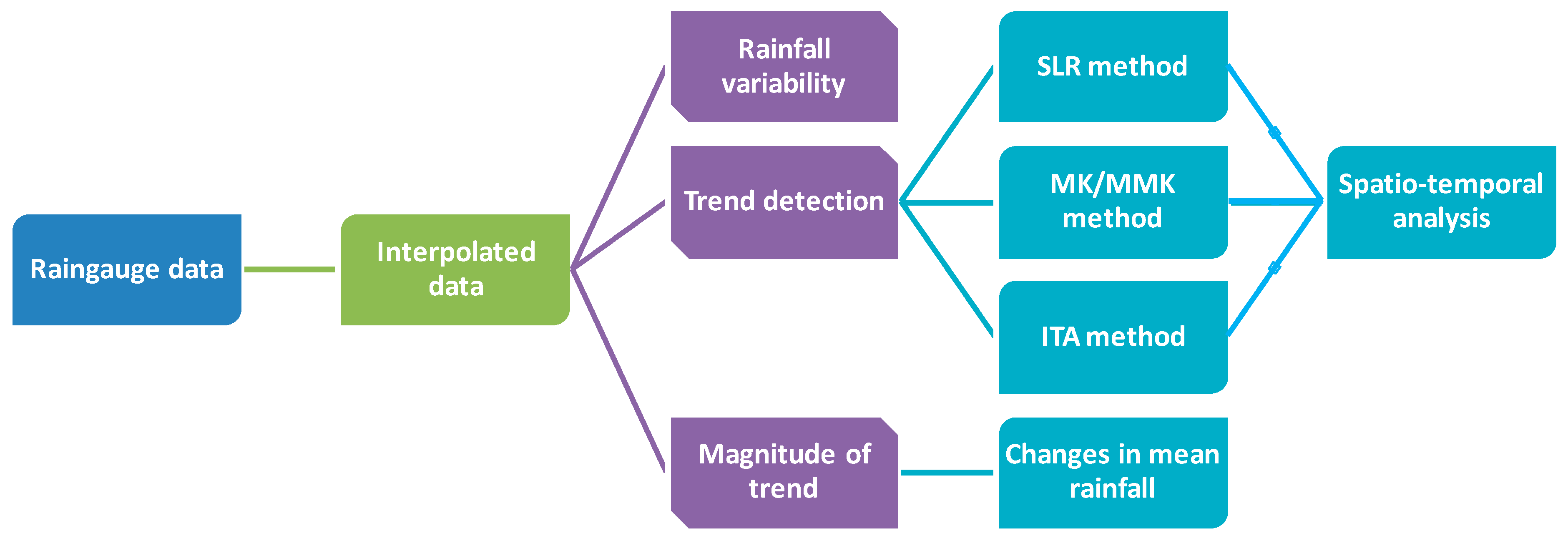
This study aims to explore the rainfall variations, spatial patterns of trends, and their magnitudes of annual and seasonal rainfall series of the Vaippar basin at micro-level using classical rainfall statistical methods. The uniqueness in this research work is the use of spatially interpolated gauge rainfall data applied at micro-level for trend detection and identification of subtrends within the rainfall series over space and time.

2. Materials and Methods

2.1. Study Area

The Vaippar River Basin, located in the southern part of Tamil Nadu, India is a significant river basin in the region. Situated between latitudes 8°97′ N and 9°78′ N and longitudes 77°24′ E and 78°37′ E, it encompasses a total catchment area of 5320 km². The basin is bounded on the north by the Vaigai and Gundar basins, on the south by the Tamaraparanibasin, on the west by the Western Ghats, and on the east by the Gulf of Mannar (Bay of Bengal). The basin area spans across four districts, with Virudhunagar accounting for 68%, Thoothukudi for 20%, Madurai for 7%, and Tirunelveli for 5% of the total area. The Vaippar River originates from the Echamalai mottai, Neduntheri mottai, and Kiladiparai hill ranges of the Western Ghats, situated near Sivagiri in Tirunelveli district. It begins at an elevation of 165 m above mean sea level and flows predominantly in an easterly and southeasterly direction for a distance of 146 km before joining the Gulf of Mannar. The catchment area of the Vaippar basin encompasses hilly regions such as Kodaliparai mottai, Vasudevanallur reserve forest, Periyasudangi malai, and others. These mountain ranges lie in the rain shadow regions of the Western Ghats, resulting in relatively low rainfall. The entire catchment area of the Vaippar basin is within the boundaries of Tamil Nadu state. The basin has been further divided into 13 sub-basins, namely: (1) Nichabanadhi, (2) Kalingalar, (3) Deviar, (4) Nagariyar, (5) Sevalperiyar, (6) Kayalkudiar, (7) VallampattiOdai/Uppodai, (8) SindapalliUppodai, (9) Arjunanadhi, (10) Kousiganadhi, (11) Uppathurar, (12) Senkottaiyar, and (13) Vaippar. The location of the Vaippar basin is depicted in Figure 1.

The basin experienced frequent drought with a range from four to eight years per drought [71]. Agricultural land covers approximately 74% of the total geographical area, while forested areas account for 10% of the area. Wasteland occupies 8% of the total geographical area, while settlements and water bodies together cover less than 8% of the basin’s total geographical area. Out of the total agriculture area in the basin, cultivable land represents 43%. This cultivable land is primarily utilized for cultivating water-intensive crops such as paddy, sugar cane, and banana [72]. Additionally, cotton, non-paddy, and dry crops are also grown in the basin. The basin’s total irrigated area accounts for 24% of the cultivable land. The remaining 76% of the cultivable land relies mainly on rainwater for irrigation [71].

2.2. Data Used

Daily rainfall data from 13 rain gauge stations distributed across the Vaippar basin were collected for this study. The data were obtained from the State Ground and Surface Water Resources Data Center, Public Works Department, and Water Resources Organization in Chennai. The location details of each rain gauge station and the period of data utilized in this study are presented in

Table 1. Details of rain gauge station geographical location and data used.

Sl. No	Rain Gauge Station	Latitude	Longitude	Elevation, m	Data Availability
1	Aruppukottai	09°30′09″	78°05′44″	123	1971–2019
2	Virudhunagar IB	09°35′00″	77°57′50″	120	1971–2019
3	Sattur	09°21′08″	77°55′13″	91	1971–2019
4	Sivakasi	09°27′44″	77°47′14″	127	1973–2019
5	Srivilliputhur	09°30′14″	77°38′08″	146	1971–2019
6	Watrap	09°38′11″	77°38′01″	73	1974–2019
7	Pilavakkal	09°38′25″	77°31′45″	141	1982–2019
8	Koilpatti (Rev)	09°10′27″	77°52′28″	130	1971–2019
9	Vilathikulam	09°07′48″	78°10′05″	47	1971–2019
10	Sankarankoil	09°10′04″	77°32′12″	143	1971–2019
11	Sivagiri	09°20′47″	77°26′01″	165	1971–2019
12	Vembakottai	09°20′06″	77°45′04″	111	2000–2019
13	Ettayapuram	09°08′53″	77°59′26″	60	1999–2019

. Standard quality control measures were undertaken to identify outliers and errors in rainfall data for all 13 rain gauges. Any potential outliers, including missing data and instrument errors, were checked and corrected. To facilitate the analysis, the daily rainfall data for each station was processed to derive monthly data. Subsequently, the monthly rainfall series was further organized into seasonal rainfall series. The seasons considered for this analysis were as follows: Southwest Monsoon (SWM) from June to September, Northeast Monsoon (NEM) from October to December, winter season in January and February, summer season from March to May, and an annual rainfall series. The space–time correlation analysis of the mean monthly rainfall data with the rain gauge stations was conducted and is presented in

Table A1. Space-time correlation analysis of the mean monthly rainfall data for Vaippar basin.

	Aruppukottai	Virudhunagar IB	Sattur	Sivakasi	Srivilliputhur	Watrap	Pilavakkal	Koilpatti (Rev)	Vilathikulam	Sankarankoil	Sivagiri	Vembakottai	Ettayapuram
Aruppukottai	1.00	0.99	0.98	0.98	0.97	0.95	0.95	0.98	0.95	0.88	0.88	0.95	0.95
Virudhunagar IB	0.99	1.00	0.97	0.97	0.95	0.93	0.93	0.96	0.93	0.84	0.84	0.95	0.94
Sattur	0.98	0.97	1.00	1.00	0.99	0.98	0.97	0.99	0.96	0.93	0.93	0.97	0.96
Sivakasi	0.98	0.97	1.00	1.00	0.99	0.99	0.98	0.99	0.96	0.93	0.93	0.97	0.97
Srivilliputhur	0.97	0.95	0.99	0.99	1.00	0.98	0.99	0.99	0.97	0.94	0.95	0.97	0.96
Watrap	0.95	0.93	0.98	0.99	0.98	1.00	0.99	0.99	0.97	0.96	0.97	0.97	0.96
Pilavakkal	0.95	0.93	0.97	0.98	0.99	0.99	1.00	0.98	0.98	0.97	0.97	0.96	0.97
Koilpatti (Rev)	0.98	0.96	0.99	0.99	0.99	0.99	0.98	1.00	0.99	0.94	0.94	0.97	0.98
Vilathikulam	0.95	0.93	0.96	0.96	0.97	0.97	0.98	0.99	1.00	0.95	0.95	0.97	0.99
Sankarankoil	0.88	0.84	0.93	0.93	0.94	0.96	0.97	0.94	0.95	1.00	1.00	0.92	0.92
Sivagiri	0.88	0.84	0.93	0.93	0.95	0.97	0.97	0.94	0.95	1.00	1.00	0.92	0.93
Vembakottai	0.95	0.95	0.97	0.97	0.97	0.97	0.96	0.97	0.97	0.92	0.92	1.00	0.98
Ettayapuram	0.95	0.94	0.96	0.97	0.96	0.96	0.97	0.98	0.99	0.92	0.93	0.98	1.00

. A strong correlation exists within the mean monthly rainfall series among the rain gauge stations.

2.3. Methodology

In this study, the monthly rainfall data collected from the 13 rain gauge stations were spatially interpolated to generate gridded rainfall data. A grid with a spacing of 0.125° in both latitude and longitude was employed to create 26 individual grids that spanned the entire basin area. The rainfall data available for each location in each year during the period specified in Table 1 underwent spatial interpolation. Using spatially interpolated monthly rainfall data, gridded rainfall data was prepared. Using the gridded rainfall data, trends in the monthly, annual, and seasonal rainfall series were estimated. Three different methods were employed for trend analysis: Mann–Kendall (MK) test, simple linear regression (SLR), and Sen’s innovative trend analysis (ITA) method. The trends were evaluated by estimating the slopes using Sen’s slope, SLR, and ITA methods to quantify the magnitude and direction of the trends in the rainfall data, and the percentage change of magnitude of trends from mean rainfall. The overall methodology used in this study is depicted as a flowchart in Figure 2.

2.4. Spatial Interpolation of Rainfall

Spatial interpolation techniques play a crucial role in estimating values at locations where no observed data is available, using known data values. Several methods, such as inverse distance weighting (IDW), splines, and kriging, are commonly employed for spatial analysis of various variables [73,74,75]. In the present study, the IDW approach was specifically utilized for spatially interpolating rainfall data across the Vaippar basin. This method considers the proximity of known data points to the location of interest and assigns weights accordingly, resulting in an interpolated surface that provides valuable insights into the spatial distribution of rainfall within the basin.

The IDW interpolation technique assigns weights to each control point based on the inverse of their distances from the interpolated point. This means that closer control points have a greater influence on the interpolated value compared to those farther away. The technique assumes that each control point has a local influence that diminishes as distance increases. In IDW interpolation, the output value at a given location is determined by a specified number of nearest points or all points within a specified radius. The power parameter of the IDW method controls the significance of the surrounding points in determining the interpolated value. A higher power value reduces the influence of distant points, resulting in a stronger emphasis on the values of nearby points in the interpolation process [76].

The general form of IDW approach [77,78] is given in Equation (1):

$$z{n}_i=\frac{{\sum }_{j=1}^m{z}_j\times d_j^{-p}}{{\sum }_{j=1}^m{d}_j^{-p}}$$

(1)

where zn_i is the new value for grid i; z_j is the value of m nearest neighbours; d_j is the distance to m nearest neighbours; p is the exponent of distance. For this study, the exponent of distance was taken as two for spatial interpolation of the rainfall.

This study employed the Inverse Distance Weighting (IDW) technique instead of the Thiessen polygon method to estimate the gridded rainfall across the basin. The Thiessen polygon method often results in a crude approximation of rainfall spatial variation due to attribute variations associated with each rain gauge station, ranging from 14 to 30% [79,80]. To overcome this limitation, the Vaippar basin was divided into smaller square grids. Given the constraints of rainfall data availability and the uneven distribution of rain gauge stations within the basin, spatial interpolation of data at smaller grids was necessary to address these challenges and obtain a more accurate representation of rainfall patterns.

The total area of the Vaippar basin was divided into 26 grids, each with dimensions of 0.125° (205 km²). These grids accounted for approximately 3.85% of the total area, equivalent to 5320 km². Monthly rainfall data recorded at 13 stations were spatially interpolated using the IDW method in QGIS 3.30.2 resulting in gridded rainfall data for the period from 1971 to 2019. The gridded rainfall data was then utilized to analyze the spatial patterns of significant trends in rainfall over the study period.

2.5. Rainfall Variability

In this study, the variability of rainfall has been assessed using the coefficient of variation (CV). The CV is a statistical measure that represents the ratio of the standard deviation to the mean of a rainfall data series. It is often used to quantify the relative variability or dispersion of rainfall. A higher CV indicates greater variability, while a lower CV suggests more stability or consistency in the data [27,81]. The CV for the rainfall events is expressed as a percentage (%). As mentioned by Hare (2003) [82], the CV can be used to classify the degree of variability of rainfall events into three categories: (i) when the CV is less than 20, rainfall events are considered to have less variability or consistent pattern of rainfall; (ii) when the CV is between 20 and 30, rainfall events are classified as having moderate variability or fluctuation; (iii) when the CV exceeds 30, rainfall events are categorized as having high variability indicating a less stable or more unpredictable rainfall.

2.6. Simple Linear Regression

Simple linear regression (SLR) analysis is a widely used parametric model for identifying monotonic long-term trends in monthly, seasonal, and annual rainfall time series [83]. SLR analysis establishes a relationship between two variables, often employed to determine the slope of hydro-meteorological variables over time. A positive slope indicates an upward trend, while a negative slope suggests a downward trend. The primary advantage of SLR analysis is its ability to provide a measure of significance through hypothesis testing on the slope, along with quantifying the rate of change. To obtain the percentage change during the specified period, the slope values are multiplied by the duration of the study period in years [16].

In this study, the simple linear regression models for the annual and seasonal time series were developed between the gridded rainfall data and time for trend detection [40,84,85]. The test statistic “t”, which follows a Student’s t-distribution with (n − 2) degrees of freedom (where “n” represents the length of the data points in the time series), was calculated to examine the significance of trend. The null hypothesis (Ho) of a zero slope is rejected when the calculated test statistic “t” value surpasses the critical value “t_α/2” at a given significance level.

2.7. Mann–Kendall (MK) Trend Analysis

The non-parametric Mann–Kendall (MK) test is a commonly used method for exploring trends in hydro-meteorological data. The trends identified by this test in the time series are monotonic, meaning they can be increasing or decreasing without assuming linearity. The test was originally proposed by Mann (1945) [86] and the test-statistic distribution was subsequently derived by Kendall (1975) [87]. The null hypothesis for this test assumes that the data is independent and randomly ordered. One advantage of this test is that it does not require any assumption of normality. However, it only indicates the direction of significant trends, without providing information about their magnitude [86,87]. The MK test statistic S indicates the number of positive differences minus the number of negative differences for all the considered differences. Using S value, its mean, and variance, the standardized test statistic Z was calculated for annul and seasonal rainfall series. A positive or negative Z value indicates an upward/downward trend [88]. The Z statistic follows a normal distribution. To test for statistical significance, compare the calculated Z value with critical values obtained from the standard normal distribution tables at two significance levels (α = 5% and α = 10%). The null hypothesis (Ho) of no trend is rejected if the calculated value of Z is greater than the table value of Z_1−α/2 [13,30,89].

2.8. Modified Mann–Kendall Test

In the Modified Mann–Kendall (MMK) test proposed by Hamed and Rao (1998) [90], the autocorrelation coefficient (ACC) of the rainfall series is computed and then subjected to testing at various levels of significance. If the ACC value is determined to be significant, the MMK test is subsequently [13,23,89].

Initially, the modified variance was computed by integrating the Auto-Covariance Correction (ACC) at lag-i. Subsequently, this modified variance was utilized in the original Mann–Kendall (MK) test, leading to the calculation of the modified Mann–Kendall Z_c statistic. To assess the significance of the trend, the modified Mann–Kendall Z_c statistic was subjected to testing against threshold levels. For instance, significance levels of 10% and 5% were represented by threshold values of 1.645 and 1.96, respectively.

2.9. Autocorrelation Analysis of Time Series

The autocorrelation (serial correlation coefficient, r) analysis is a useful tool for evaluating the presence of randomness and periodicity within a time series at different lag periods [91]. To calculate autocorrelation coefficients (ACC), the normalized anomaly of the rainfall series, obtained from gridded rainfall data, along with the long-term average and standard deviation of annual and seasonal rainfall, can be utilized. Positive or negative ACC values are generally influenced by the trends identified in the time series [90,92,93]. If the ACC is close to zero for different time lags, it suggests that the data points in the time series are randomly distributed, indicating no dependence. On the other hand, the presence of serial correlation, as examined through autocorrelation analysis, is an important preliminary test before performing the Mann–Kendall (MK) trend analysis. This is because the MK analysis requires the input data to be serially independent. Otherwise, the presence of positive serial correlation in the data can lead to an overestimation of trend significance. The lag-1 ACC specifically detects the serial correlation in the data series. The statistical significance of serial correlation can be tested by employing a normally distributed statistic at a significance level of “α”, taking into account the lag period and the length of the series [94].

The ACC (r_k) of the rainfall time series at lag-k can be computed using the rainfall data of the time series and the total length of the time series, where “k” represents the time lag. The value of r_k ranges between +1 and −1. A value of zero for r_k signifies that the series is random for all lag-k values [15]. To evaluate the statistical significance of the ACC in the time series data, testing should be conducted at both upper and lower confidence limits. If the ACC turns out to be statistically insignificant, the Mann–Kendall (MK) test can then be applied to the original time series [95,96]. The null hypothesis (Ho) suggests the absence of serial correlation within the time series, while the alternative hypothesis (Ha) suggests the presence of some serial correlation rather than pure randomness. In this study, the hypothesis was examined using the lag-1 autocorrelation coefficient. The upper and lower confidence limits can be calculated [45,97] at a significance level denoted as α (e.g., for α = 10%, Z = ±1.645, and for α = 5%, Z = ±1.96) [45]. When the r_k value falls within the range of the critical values {(r_k) upper < r_k < (r_k) lower}, the null hypothesis Ho: r_k = 0 is rejected, while Ha: r_k ≠ 0 is accepted. This indicates that the time series is not random and exhibits some level of persistence or serial correlation [11].

2.10. Sen’s Slope

The magnitude of trends in monthly, seasonal, and annual time series was determined using Sen’s slope, a non-parametric method introduced by Sen (1968) [98]. Sen’s slope requires equally spaced data in a time series [11]. One of the main advantages of Sen’s slope over simple linear regression (SLR) is its resilience to data errors, outliers, and extreme observations [15]. This method is particularly useful when assuming a linear trend line.

The slope estimate Q for each pair of data values is calculated using $Q_i=median\frac{x_j-x_k}{j-k}$ where x_j and x_k are the data values at time j and k, respectively (j > k). If there are n data values x_j in the time series, there will be a total of N = n(n − 1)/2 slope estimates Q_i. The N values of Q_i are then ranked from the smallest to the largest. The Sen’s slope is determined based on whether N is odd or even: if N is odd, the Sen’s slope is $=Q_{\left[\frac{(N+1)}{2}\right]}$; if N is even, the Sen’s slope is $Q=\frac{1}{2}\left(Q_{\left[\frac{N}{2}\right]}+Q_{\left[\frac{(N+2)}{2}\right]}\right)$. A positive value of Q indicates an upward trend, while a negative value represents a downward trend. A Q value of zero indicates no trend in the time series [15,30].

2.11. Innovative Trend Analysis

The Innovative Trend Analysis (ITA) method has been successfully utilized for trend detection in hydro-meteorological variables [8,52]. This method is simple, allowing for easy identification and visualization of trends in high, medium, and low data set on the trend line [70]. Unlike non-parametric trend identification tests, the ITA method does not require restrictive assumptions such as data series independence, normality, or data length [8,47,99]. It involves plotting all data points of the time series in a Cartesian coordinate system and comparing them with a diagonal straight 1:1 line [44,100]. The construction procedure for ITA is provided below:

(a)

Divide the monthly, annual, or seasonal rainfall time series into two equal halves. Arrange each half series in ascending order.

(b)

Place the first half of the time series on the X-axis and the second half on the Y-axis. Plot the rainfall series as a scatter diagram.

(c)

Draw a straight 45° line diagonally in the scatter graph representing a 1:1 relationship. Divide the plot into upper and lower half triangles.

(d)

If the scattered points align perfectly on the 45° line, the series does not exhibit a trend.

(e)

When the scattered points lie within the upper half triangle, the rainfall series is said to have an increasing trend.

(f)

When the scattered points lie within the lower half triangle, the rainfall series is said to have a decreasing trend.

(g)

A time series is considered to have a monotonic trend if all scattered points lie above or below the upper or lower half triangles. Non-monotonic trends occur when some scattered points are located in the upper half triangle and others in the lower half triangles [8].

(h)

The trend of low, medium, and high values can be observed in the scatter graph.

(i)

To test the significance of the trend, a null hypothesis (Ho) is considered: there is no significant trend if the calculated slope value (S) is below the critical value (S_cri). The alternative hypothesis (Ha) states that there is a significant trend when S > S_cri.

(j)

The slope (S) of the trend is computed using the formula [101]:

$$S=\frac{2({\overline{y}}_2-{\overline{y}}_1)}{n}$$

(2)

where, ${\overline{y}}_1$ and ${\overline{y}}_2$ represent the mean of the first and second halves of the rainfall time series, and n is the number of data points in the rainfall time series.

(k)

The standard deviation (σ_s) of the trend slope is calculated using the formula [101]:

$${\sigma }_S=\frac{2\sqrt{2}}{n\sqrt{n}}\sigma \sqrt{1-{\rho }_{{\overline{y}}_1{\overline{y}}_2}}$$

(3)

where σ represents the standard deviation and ${\rho }_{{\overline{y}}_1{\overline{y}}_2}$ is the cross-correlation coefficient between the means of the two-half series.

(l)

By utilizing the confidence limits (S_cri) for a standard normal probability density function, the confidence limits of the trend slope are calculated at a significance level of α using the formula [101]:

$${CL}_{(1-\alpha )}=0\pm S_{cri}{\sigma }_S$$

(4)

If the slope value (S) falls beyond the lower or upper confidence limits, the null hypothesis of no significant trend is rejected at the α significance level.

2.12. Percentage Change in Magnitude of Trend from Mean Rainfall

The percentage change in magnitude of trend from mean rainfall of seasonal and annual time series can be calculated using the following expression [31,102,103]:

$$PC=\frac{n\times S}{\overline{x}}\times 100$$

(5)

where PC represents the percentage change of rainfall (%), n is the length of time series in years, S is the magnitude of the trend slope calculated using methods such as Simple Linear Regression (SLR) coefficient, Sen’s slope, or Innovative Trend Analysis (ITA) slope, and $\overline{x}$ is the mean value of the time series. This equation allows for quantifying the percentage of change in rainfall over the specified time period, relative to the mean value of the time series.

3. Results and Discussion

3.1. Rainfall Variability

The mean rainfall and coefficients of variation (CV) for the monthly, seasonal, and annual rainfall of 26 grid points in Vaippar during the period 1971–2019 is presented in

Table A2. Mean rainfall of 26 grid points of Vaippar during the period 1971–2019.

Grid	JAN	FEB	MAR	APR	MAY	JUN	JUL	AUG	SEP	OCT	NOV	DEC	ANL	SWM	NEM	WIN	SUM
G01	22.18	43.25	50.90	81.96	55.67	14.96	19.69	27.93	66.92	199.76	224.74	79.04	886.99	129.49	503.54	65.43	188.53
G02	22.00	42.61	49.84	81.78	54.04	14.56	18.99	26.28	63.51	197.34	224.12	78.81	873.89	123.34	500.27	64.61	185.67
G03	18.89	29.84	40.00	70.40	51.94	12.36	16.95	24.75	55.81	181.46	197.44	70.52	770.37	109.87	449.42	48.73	162.34
G04	19.80	31.98	48.08	67.83	64.85	13.91	26.28	41.50	88.98	199.81	200.66	72.82	876.48	170.67	473.28	51.78	180.75
G05	19.05	29.51	45.49	68.58	67.14	14.65	22.12	38.34	83.47	196.20	191.58	70.00	846.13	158.58	457.78	48.56	181.21
G06	19.68	34.63	46.03	73.70	60.67	14.55	20.15	32.15	72.51	194.99	202.26	72.57	843.87	139.35	469.81	54.31	180.40
G07	19.55	33.11	42.82	73.35	53.58	13.07	17.72	26.07	59.56	186.79	203.54	72.29	801.44	116.41	462.62	52.66	169.74
G08	25.51	25.65	45.31	79.12	67.80	15.35	20.23	40.25	92.87	208.40	205.55	65.88	891.93	168.71	479.82	51.16	192.24
G09	15.81	27.84	47.92	66.23	76.73	15.46	19.72	38.90	86.84	196.78	178.65	69.87	840.75	160.92	445.30	43.65	190.88
G10	16.63	25.80	40.64	65.32	67.02	14.22	20.78	37.09	79.75	189.99	175.04	64.40	796.69	151.85	429.43	42.43	172.98
G11	17.06	24.46	36.05	64.55	57.29	12.57	19.64	32.02	67.87	185.25	177.31	63.62	757.69	132.10	426.19	41.51	157.89
G12	19.15	23.62	38.16	66.06	66.58	15.60	24.27	42.64	85.95	190.10	174.33	62.67	809.13	168.46	427.10	42.77	170.80
G13	15.57	22.31	34.67	61.23	64.34	14.63	21.28	40.27	82.27	177.51	158.50	56.86	749.44	158.45	392.87	37.88	160.24
G14	14.76	20.81	31.94	59.79	61.21	13.41	20.52	38.90	78.84	174.98	151.93	53.26	720.35	151.67	380.17	35.57	152.94
G15	16.19	19.62	31.28	59.98	58.42	12.26	22.37	36.56	75.28	186.68	159.39	56.34	734.37	146.48	402.41	35.80	149.68
G16	17.99	18.73	30.02	59.67	69.42	18.60	33.59	53.97	88.20	180.10	149.19	59.52	778.99	194.36	388.81	36.72	159.11
G17	16.95	18.40	29.32	58.66	68.04	17.71	31.64	51.50	86.27	176.19	146.39	57.78	758.84	187.12	380.36	35.35	156.01
G18	14.38	17.26	29.01	57.64	63.38	12.47	24.38	39.20	77.10	163.33	142.84	55.22	696.21	153.15	361.39	31.64	150.03
G19	14.92	17.78	27.69	56.21	59.90	12.04	23.45	36.04	76.75	171.44	147.70	57.47	701.40	148.29	376.61	32.70	143.80
G20	16.52	16.79	26.12	52.61	70.60	21.63	37.44	55.51	87.49	173.36	141.51	57.78	757.36	202.07	372.64	33.31	149.33
G21	15.00	17.38	27.32	53.11	64.39	16.61	29.28	43.77	79.75	169.04	144.58	57.07	717.31	169.42	370.69	32.38	144.82
G22	14.61	17.85	25.99	52.24	56.03	12.49	23.86	36.39	74.35	172.80	147.23	58.18	692.02	147.09	378.21	32.46	134.27
G23	13.17	18.41	21.10	43.85	41.90	9.65	20.30	31.26	69.60	181.73	149.37	59.88	660.22	130.82	390.98	31.57	106.85
G24	14.25	17.40	23.90	47.20	49.98	12.29	22.99	34.23	68.88	173.48	146.12	59.21	669.93	138.40	378.81	31.65	121.08
G25	12.32	14.87	16.83	36.82	29.83	6.03	14.82	21.26	49.77	169.76	137.85	60.04	570.20	91.88	367.65	27.19	83.49
G26	13.51	16.78	21.11	42.77	39.40	8.80	18.23	27.03	59.17	173.16	144.70	60.26	624.92	113.22	378.12	30.29	103.28
Mean	17.13	24.10	34.91	61.56	59.24	13.84	22.72	36.68	75.30	183.48	170.10	63.51	762.57	148.54	417.09	41.23	155.71
Max	25.51	43.25	50.90	81.96	76.73	21.63	37.44	55.51	92.87	208.40	224.74	79.04	891.93	202.07	503.54	65.43	192.24
Min	12.32	14.87	16.83	36.82	29.83	6.03	14.82	21.26	49.77	163.33	137.85	53.26	570.20	91.88	361.39	27.19	83.49

and

Table A3. Coefficientof variation (CV) of gridded rainfall of Vaippar during the period 1971–2019.

Grid	JAN	FEB	MAR	APR	MAY	JUN	JUL	AUG	SEP	OCT	NOV	DEC	ANL	SWM	NEM	WIN	SUM
G01	154.18	140.78	140.79	69.21	91.50	102.63	80.10	91.22	71.29	53.74	49.67	101.42	26.95	46.25	32.90	113.22	53.25
G02	154.74	139.89	138.83	69.96	94.30	105.85	82.42	94.61	72.52	54.00	50.78	100.41	27.63	47.19	34.09	112.88	53.40
G03	160.41	137.16	140.52	63.02	75.10	112.95	100.21	89.63	67.49	46.10	55.65	95.75	26.17	43.89	37.44	108.60	46.61
G04	209.10	182.91	206.47	80.43	69.20	113.19	114.17	106.91	78.25	49.97	66.26	114.12	29.46	50.34	38.46	139.66	60.61
G05	191.89	157.09	178.35	62.38	56.22	95.67	95.11	80.86	72.20	47.33	54.61	98.78	24.43	45.78	31.90	123.93	48.79
G06	160.84	141.70	151.16	60.03	67.25	93.40	75.63	80.00	68.33	46.81	48.89	96.89	22.94	43.33	29.84	112.37	46.94
G07	155.48	137.10	140.31	62.92	76.39	106.01	86.15	87.91	67.81	46.82	52.82	95.45	25.17	43.49	34.81	108.77	47.20
G08	200.29	166.11	173.00	92.12	68.03	145.89	124.84	107.60	86.24	61.20	66.99	124.10	30.73	62.13	41.84	127.38	54.12
G09	243.12	168.77	192.18	67.97	67.11	119.19	114.92	101.25	99.80	57.18	62.06	102.65	31.47	65.83	34.56	139.72	57.57
G10	206.11	157.07	172.22	62.59	57.03	99.49	95.52	82.48	74.52	49.04	57.88	95.36	25.49	47.76	32.55	129.16	46.71
G11	177.12	145.75	151.89	62.93	57.59	97.41	90.44	82.70	62.11	44.84	55.16	91.14	23.78	40.22	33.72	118.37	43.56
G12	202.91	159.49	170.31	73.56	53.73	93.63	92.76	74.55	64.21	50.10	60.93	102.03	25.17	41.53	35.90	129.36	45.64
G13	219.95	173.14	171.89	78.27	63.15	105.55	111.57	90.21	63.59	52.38	71.66	101.21	28.72	45.23	40.31	141.20	47.20
G14	221.81	180.04	170.45	84.47	66.34	116.36	121.05	96.20	63.59	53.58	76.03	101.18	30.76	46.86	41.89	146.75	49.54
G15	207.47	159.99	162.01	73.34	52.34	104.70	103.38	87.00	60.13	49.81	61.49	92.45	26.41	41.89	36.42	134.90	46.51
G16	240.21	176.93	164.07	79.87	59.33	91.70	99.24	72.57	60.10	52.27	70.09	98.48	25.71	38.72	40.16	156.94	46.74
G17	243.80	178.31	163.36	78.11	59.17	91.64	100.12	73.89	57.23	51.61	71.25	97.91	25.80	37.95	40.30	157.86	45.87
G18	240.03	168.06	161.48	75.01	61.88	117.59	115.62	84.21	60.44	49.76	70.27	101.75	27.11	44.30	41.60	146.09	43.58
G19	232.13	155.85	159.91	72.59	61.30	114.08	109.24	83.74	58.03	46.93	65.70	94.24	25.52	41.91	38.84	138.89	43.57
G20	263.69	185.11	162.49	77.40	60.18	98.01	91.04	70.86	58.72	59.35	70.12	102.95	27.89	36.83	43.16	171.22	45.30
G21	244.70	164.01	160.37	71.41	57.94	101.21	90.37	70.06	55.71	52.92	65.67	100.62	26.47	36.59	40.27	150.53	41.90
G22	230.41	155.91	162.05	70.61	59.99	101.53	96.35	77.20	53.96	48.78	61.95	94.59	24.96	37.78	37.39	140.41	42.90
G23	239.88	175.30	180.07	81.78	77.29	113.59	111.86	98.10	54.59	59.61	60.99	96.21	29.18	41.43	40.09	153.86	56.02
G24	215.48	155.79	165.05	71.72	63.30	92.52	92.20	75.02	49.83	49.43	56.85	95.00	24.11	33.88	34.54	139.31	44.42
G25	199.82	191.86	189.23	114.12	117.77	155.16	143.20	111.09	65.75	54.41	56.78	105.52	28.19	46.33	33.84	159.45	70.67
G26	197.54	161.72	172.00	83.18	80.17	100.07	108.34	86.91	51.53	50.12	54.14	97.53	24.51	35.94	32.51	140.05	52.09

. During the study period, the Vaippar basin experienced an annual average rainfall of 762.57 mm. The highest rainfall of 891.93 mm was observed in the G08 grid point, while the lowest rainfall of 570.2 mm occurred in the G18 grid point. Out of 26 grid points, 12 grid points located mostly on the western side of the basin experienced annual rainfall that exceeded the average annual rainfall. The NEM is the major rainy season in the study area, contributing approximately 54.7% of the annual rainfall. Within the NEM season, the majority of the rainfall, around 85%, occurred in two months: October and November. The month of December contributed to approximately 15% of the summer rainfall. Among the grid points, the highest NEM rainfall of 503.54 mm was recorded in the G01 grid point, while the lowest NEM rainfall of 361.39 mm was recorded in the G18 grid point. Apart from the NEM season, the remaining seasons, namely SWM, winter, and summer, contributed 19.5%, 5.4%, and 20.4% of the annual rainfall, respectively. The maximum monthly rainfall was observed in October, accounting for 24.1% of the annual rainfall. The month of November followed closely with 22.3% contribution, while September contributed 9.9%, and December contributed 8.3% of the annual rainfall.

In the Nagariyar sub basin (G01 grid point), the maximum rainfall was recorded during the months of February, March, April, November, December, and the winter season. The G08 grid point (part of Arjunanadhi) experienced high rainfall in January, September, and October, annually, and during the summer season. On the other hand, the G20 grid point (part of Kousiganadhi) recorded higher rainfall in June, July, August, and during the Southwest Monsoon (SWM) season. The grid points located in the lower part of the Sinkottaiyar sub basin (G25) and Sindapalli Uppodai sub basin (G14 and G18) registered the minimum rainfall. The G25 grid point recorded the minimum monthly rainfall from January to September, November, SWM, winter, and summer seasons. The G18 grid point experienced the minimum rainfall during October, while the G14 grid point recorded the minimum rainfall in December.

The coefficient of variation (CV) of monthly, seasonal, and annual rainfall calculated for each grid point is shown in Table A3. Rainfall variability as classified by Hare (2003) [82], shows the CV for annual mean rainfall ranges from 22.9% to 31.5%, indicating moderate to high variability in rainfall distribution across all grids. The G09 grid point recorded the highest CV, while the G06 grid point recorded the lowest CV for annual rainfall. Most of the grid points exhibited moderate variability in annual rainfall, except for G08, G09, and G14, which are located at the centre of the basin. Rainfall variability was found to be greater in seasonal rainfall compared to annual rainfall. However, it is worth noting that the NEM season experienced relatively lower variability compared to the other seasons. Among the months, October (51.47%) and November (61.33%) exhibited lower coefficients of variation (CV) compared to the other months.

3.2. Trends of Annual and Seasonal Rainfall Series

The temporal trends were identified using the SLR, MK/MMK, and ITA methods at different grid points of Vaippar basin for annual and seasonal rainfall series. The calculated values of the SLR t test, MK/MMK test statistic (Z test), and ITA (slope values) were spatially mapped for each grid point by IDW interpolation method using QGIS 3.30.2 software. The magnitude of the trends was identified and percentage changes in mean rainfall were also calculated. The comparison of number of grid points expressing the significant trends and correlation among the different trend methods were also attempted. The results are discussed in the subsequent sections.

3.3. Trends of Annual and Seasonal Rainfall Series by Simple Linear Regression

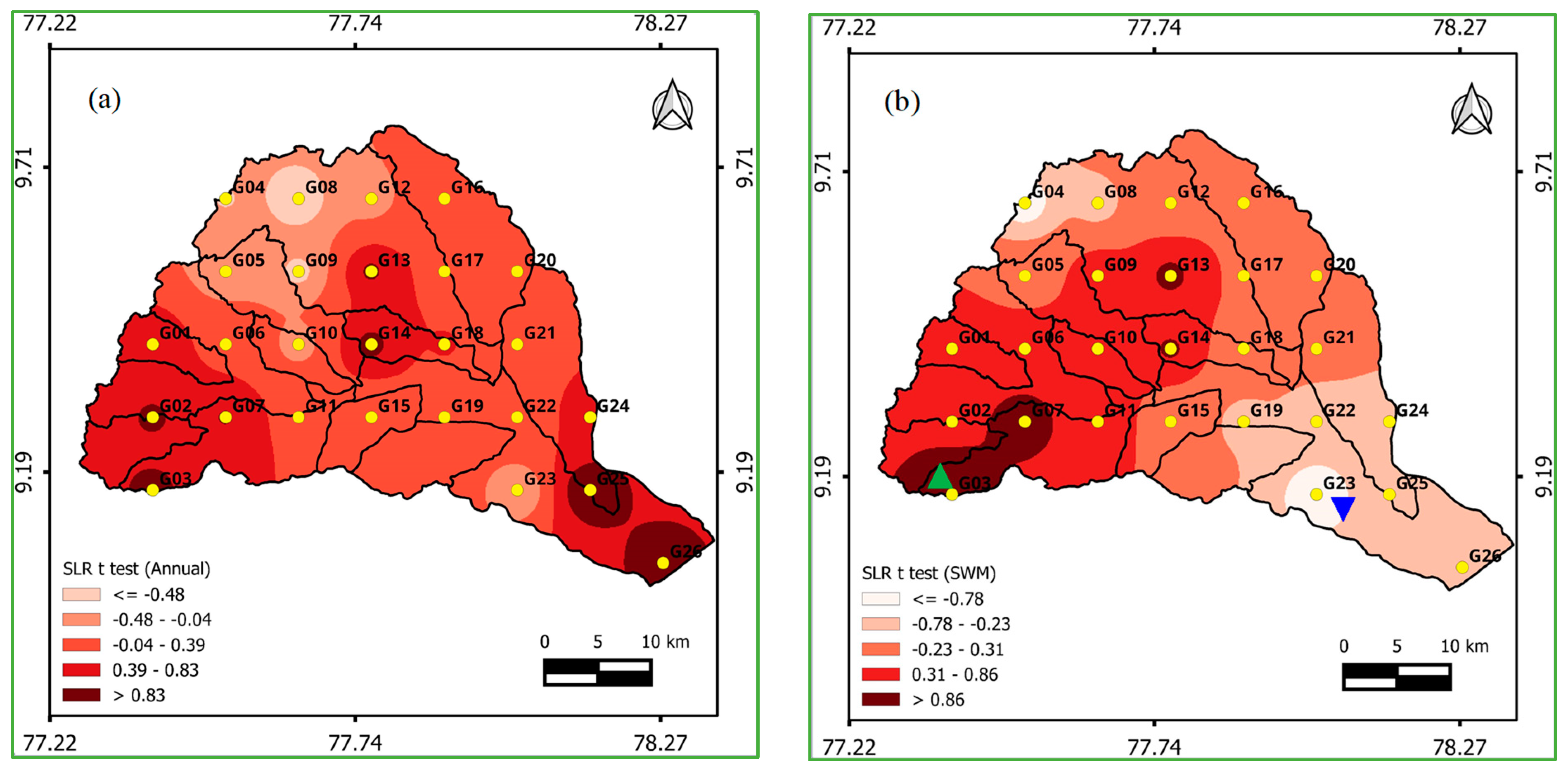
The spatial distributions of trends in annual and seasonal rainfall, detected by the SLR method at the 5% and 10% significance levels, are shown in Figure 3. The analysis of temporal trends using the simple linear regression for annual and seasonal rainfall series showed that approximately 73% of grid points exhibited non-significant upward trends in the annual rainfall series. Although the NEM rainfall is a major contributor to the annual rainfall, the trend pattern was not similar, with 50% of grid points showing a non-significant downward trend. The winter and summer rainfall series demonstrated that 57.7% and 76.9% of grid points, respectively, displayed non-significant upward trends.

Among the five-rainfall series (annual and seasonal), only two series (SWM and summer) exhibited 7.69% of significant trends at the extreme ends of the basin. In the SWM series, an upward trend was observed at the G03 grid point and a downward trend at the G23 grid point, both at a 10% significance level. The summer rainfall series showed an upward trend at the G01, G02, G14, and G26 grid points at a 10% significance level, and at the G04, G07, and G25 grid points at a 5% significance level. A significant downward trend was noticed at the G23 grid point for the summer series. Consequently, the expected decrease in rainfall will not have a significant impact on water availability, as these seasons contribute very little to the annual rainfall.

3.4. Trends of Annual and Seasonal Rainfall Series by MK/MMK Test

The Mann–Kendall (MK) method was applied to the annual and seasonal rainfall series at different grid points of the Vaippar basin to identify significant trends at the 5% and 10% significance levels using the Z-test. The MK test was conducted for the annual and seasonal series, taking into account the auto-correlated non-significant series at lag-1. The modified MK (Z_c) test was performed only for statistically significant auto-correlated series.

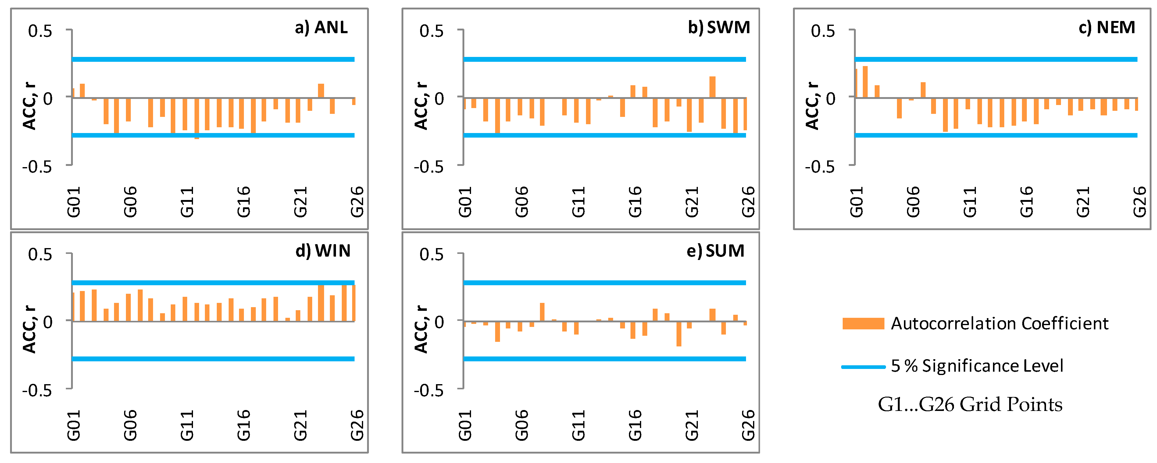
Autocorrelation analysis was conducted to select the appropriate trend analysis method and evaluate the performance of both the original and normalized rainfall series. The autocorrelation coefficient for 26 grid points at lag-1 period for annual and seasonal rainfall series were worked out and the correlogram is presented in Figure 4. The upper and lower bound were decided by the 95% confidence interval to test the limits of the autocorrelation coefficient. The autocorrelation was considered as significant if it is greater than or lower than ±0.28. Since autocorrelation was found to be significant for five rainfall series viz ANL-G10, ANL-G12, SWM-G25, WIN-G23 and WIN-G25, the modified MK test was performed for these five series.

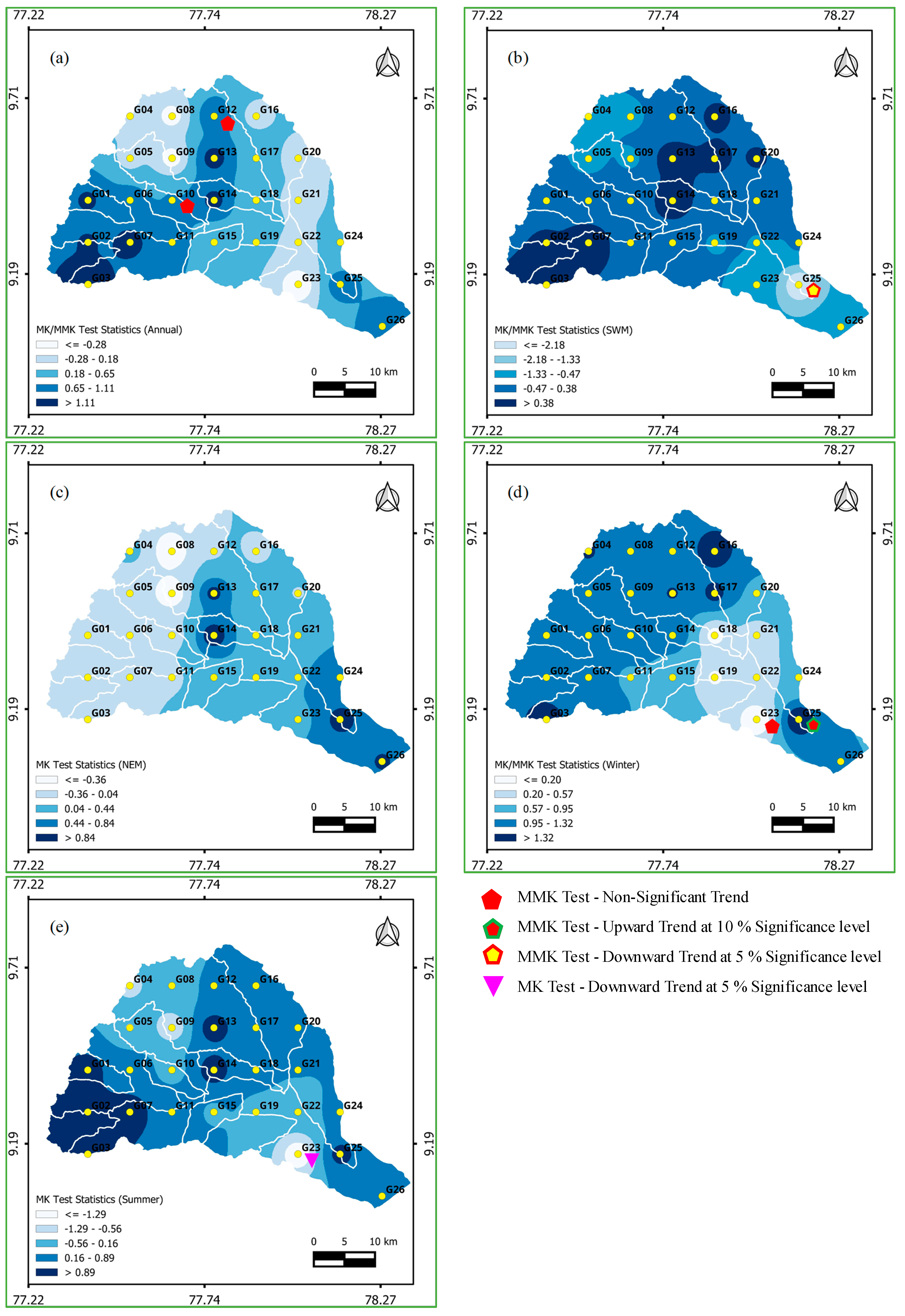
The spatial pattern of trends in annual and seasonal rainfall, identified using the MK methods, is presented in Figure 5. Compared to the SLR test and ITA method, very few statistically significant trends were observed in the annual and seasonal rainfall series for both the MK and MMK tests. The temporal patterns of trend detected by MK test indicated that approximately 73% of the grid points for the annual series and 58% of the grid points for the NEM series showed non-significant upward trends. Furthermore, 54% of the grid points for the SWM series displayed a non-significant downward trend.

The MK test detected a downward trend at the 5% significance level in the G23 grid point for the summer series. A total of five rainfall series were tested using the modified MK method, which detected a significant downward trend at the G23 grid point for the SWM series, while the same grid point exhibited a significant upward trend for the winter season.

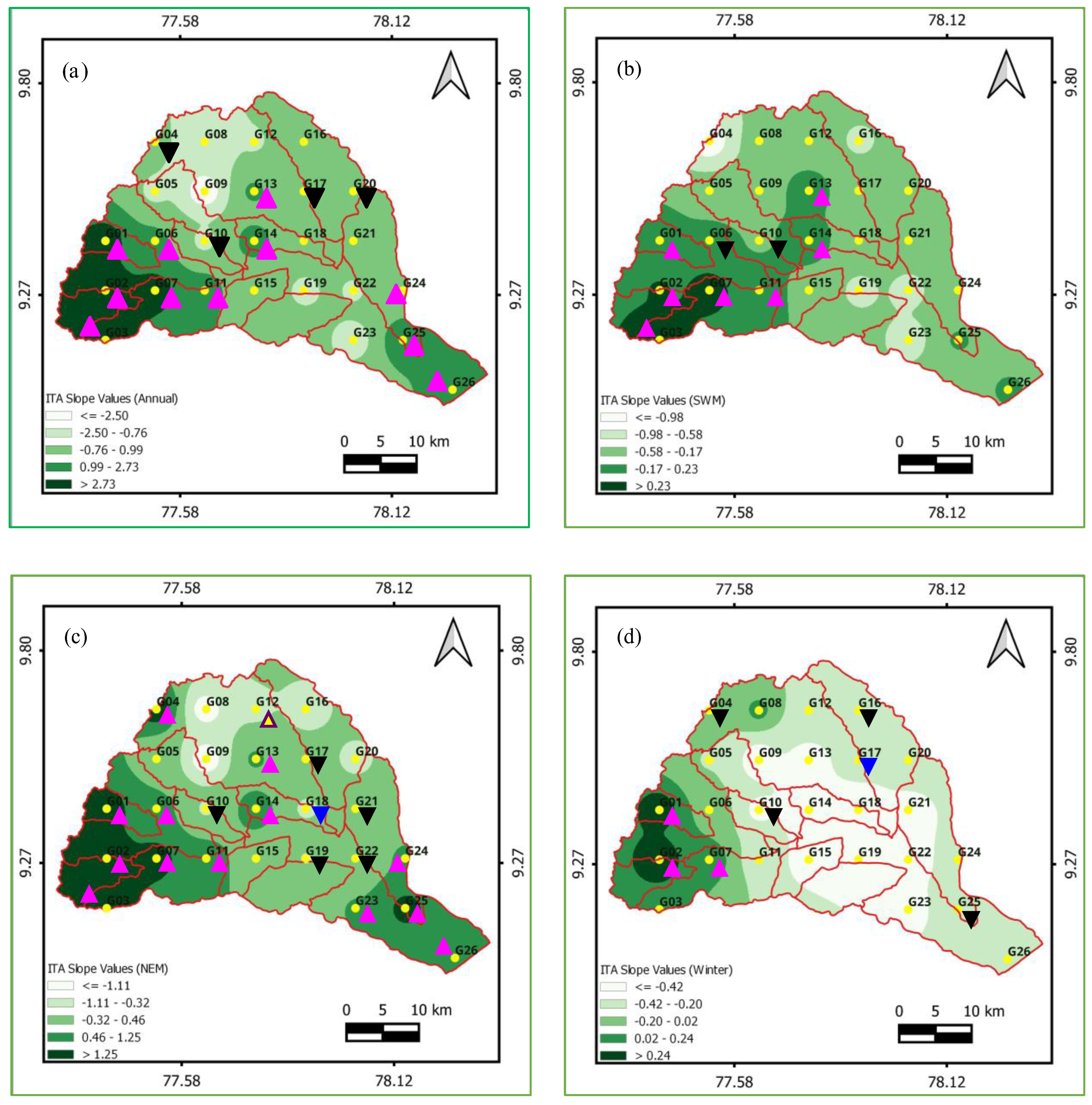
3.5. Trends of Annual and Seasonal Rainfall Series by ITA Method

The grid-wise trend parameters for the annual and seasonal rainfall series of the Vaippar basin, as detected by the ITA method, are presented in

Table 2. Grid-wise trend parameters detected by the ITA method for the annual and SWM rainfall series of the Vaippar basin.

Grid	Annual Series							SWM Series
	S	σ	ρ	σs	LCL	UCL	Decision	S	σ	ρ	σs	LCL	UCL	Decision
G01	3.85	239.07	0.94	0.47	±0.77	±0.92	Ha **	0.13	59.89	0.98	0.06	±0.11	±0.13	Ha **
G02	4.47	241.49	0.95	0.47	±0.77	±0.91	Ha **	0.26	58.2	0.98	0.06	±0.10	±0.12	Ha **
G03	4.42	201.58	0.91	0.5	±0.82	±0.97	Ha **	0.64	48.23	0.96	0.08	±0.13	±0.16	Ha **
G04	−0.44	258.21	0.89	0.7	±1.16	±1.38	−Ha **	−1.39	85.92	0.97	0.13	±0.21	±0.25	Ho
G05	−1.11	206.69	0.96	0.36	±0.59	±0.71	Ho	−0.53	72.59	0.97	0.10	±0.16	±0.19	Ho
G06	1.41	193.6	0.92	0.44	±0.72	±0.86	Ha **	−0.01	60.38	0.95	0.11	±0.18	±0.21	−Ha **
G07	4.03	201.73	0.93	0.43	±0.72	±0.85	Ha **	0.5	50.63	0.97	0.07	±0.11	±0.13	Ha **
G08	−2.48	274.13	0.97	0.36	±0.59	±0.70	Ho	−0.5	104.81	0.97	0.16	±0.26	±0.31	Ho
G09	−4.24	264.56	0.92	0.6	±0.98	±1.17	Ho	−0.42	105.93	0.98	0.12	±0.20	±0.24	Ho
G10	−1.21	203.12	−0.27	1.89	±3.10	±3.70	−Ha **	−0.22	72.52	−0.19	0.65	±1.07	±1.28	−Ha **
G11	1.62	180.2	0.91	0.45	±0.74	±0.88	Ha **	0.23	53.13	0.94	0.11	±0.18	±0.21	Ha **
G12	−0.86	203.68	0.97	0.27	±0.44	±0.52	Ho	−0.41	69.96	0.97	0.1	±0.16	±0.19	Ho
G13	1.43	215.23	0.99	0.21	±0.35	±0.42	Ha **	0.19	71.67	0.97	0.11	±0.18	±0.21	Ha *
G14	2.05	221.59	0.98	0.23	±0.38	±0.46	Ha **	0.2	71.07	0.97	0.1	±0.17	±0.20	Ha **
G15	0.1	193.97	0.97	0.28	±0.46	±0.55	Ho	−0.37	61.36	0.96	0.11	±0.17	±0.21	Ho
G16	−0.77	200.28	0.99	0.2	±0.33	±0.39	Ho	−0.67	75.26	0.96	0.12	±0.19	±0.23	Ho
G17	−0.24	195.79	0.98	0.21	±0.34	±0.41	−Ha **	−0.51	71.02	0.96	0.12	±0.20	±0.24	Ho
G18	−0.72	188.77	0.98	0.23	±0.38	±0.45	Ho	−0.51	67.84	0.93	0.15	±0.25	±0.29	Ho
G19	−1.15	179.03	0.96	0.28	±0.47	±0.56	Ho	−0.72	62.15	0.95	0.11	±0.19	±0.22	Ho
G20	−0.47	211.24	0.96	0.37	±0.60	±0.72	−Ha **	−0.45	74.42	0.97	0.11	±0.19	±0.22	Ho
G21	−0.55	189.85	0.98	0.21	±0.34	±0.4	Ho	−0.47	61.99	0.96	0.1	±0.16	±0.19	Ho
G22	−0.94	172.76	0.97	0.25	±0.41	±0.48	Ho	−0.7	55.57	0.96	0.09	±0.15	±0.18	Ho
G23	−1.54	192.63	0.96	0.32	±0.52	±0.63	Ho	−0.76	54.19	0.96	0.09	±0.15	±0.18	Ho
G24	0.44	161.5	0.97	0.23	±0.37	±0.44	Ha *	−0.37	46.9	0.99	0.04	±0.07	±0.09	Ho
G25	2.35	160.77	0.97	0.23	±0.38	±0.46	Ha **	−0.13	42.57	0.98	0.05	±0.09	±0.11	Ho
G26	1.63	153.19	0.97	0.21	±0.35	±0.41	Ha **	−0.15	40.69	0.97	0.06	±0.10	±0.12	Ho

S—ITA slope; σ—standard deviation; ρ—correlation coefficient between the means of two half series; σs—standard deviation of trend slope; LCL/UCL—lower/upper confidence limits; Ho: no significant trend; Ha: there is a significant trend; **—significance level at 5 and 10%; *—significance level at 5%.

,

Table 3. Grid-wise trend parameters detected by the ITA method for the NEM and winter rainfall series of the Vaippar basin.

Grid	NEM Series							Winter Series
	S	σ	ρ	σs	LCL	UCL	Decision	S	σ	ρ	σs	LCL	UCL	Decision
G01	1.8	165.65	0.97	0.25	±0.41	±0.49	Ha **	0.42	74.07	0.95	0.14	±0.23	±0.27	Ha **
G02	2.03	170.53	0.97	0.23	±0.38	±0.45	Ha **	0.46	72.93	0.95	0.13	±0.22	±0.26	Ha **
G03	1.79	168.28	0.93	0.36	±0.60	±0.71	Ha **	0.21	52.93	0.9	0.14	±0.22	±0.27	Ho
G04	1.85	182.03	0.99	0.18	±0.30	±0.35	Ha **	−0.04	72.31	0.98	0.08	±0.13	±0.15	−Ha **
G05	0.01	146.05	0.97	0.21	±0.34	±0.40	Ho	−0.21	60.18	0.98	0.07	±0.11	±0.13	Ho
G06	0.71	140.19	0.98	0.16	±0.27	±0.32	Ha **	0.01	61.02	0.97	0.09	±0.15	±0.18	Ho
G07	1.69	161.06	0.95	0.28	±0.47	±0.55	Ha **	0.22	57.28	0.94	0.11	±0.19	±0.22	Ha *
G08	−1.61	200.77	0.97	0.29	±0.48	±0.57	Ho	0.09	65.16	0.93	0.14	±0.24	±0.28	Ho
G09	−1.89	153.9	0.96	0.25	±0.42	±0.50	Ho	−0.62	60.99	0.97	0.08	±0.13	±0.16	Ho
G10	−0.43	139.8	−0.15	1.24	±2.04	±2.43	−Ha **	−0.48	54.8	−0.12	0.48	±0.79	±0.94	−Ha **
G11	0.73	143.7	0.97	0.22	±0.35	±0.42	Ha **	−0.28	49.13	0.93	0.11	±0.18	±0.21	Ho
G12	−0.42	153.33	0.96	0.25	±0.41	±0.49	Ha #	−0.26	55.33	0.98	0.06	±0.11	±0.13	Ho
G13	0.61	158.35	0.98	0.2	±0.33	±0.40	Ha **	−0.54	53.49	0.90	0.14	±0.23	±0.27	Ho
G14	1.05	159.23	0.96	0.25	±0.41	±0.49	Ha **	−0.64	52.20	0.87	0.15	±0.25	±0.30	Ho
G15	0.31	146.56	0.97	0.19	±0.32	±0.38	Ho	−0.55	48.30	0.85	0.15	±0.25	±0.30	Ho
G16	−0.58	156.15	0.96	0.26	±0.43	±0.51	Ho	−0.24	57.62	0.78	0.22	±0.36	±0.43	−Ha **
G17	−0.32	153.28	0.97	0.23	±0.37	±0.45	−Ha **	−0.34	55.80	0.82	0.2	±0.32	±0.38	−Ha #
G18	−0.45	150.33	0.95	0.27	±0.44	±0.53	−Ha #	−0.6	46.23	0.92	0.11	±0.18	±0.22	Ho
G19	−0.36	146.27	0.96	0.24	±0.40	±0.47	−Ha **	−0.57	45.41	0.90	0.12	±0.20	±0.24	Ho
G20	−0.47	160.83	0.97	0.22	±0.36	±0.43	Ho	−0.3	57.04	0.93	0.12	±0.20	±0.24	Ho
G21	−0.25	149.28	0.97	0.2	±0.33	±0.40	−Ha **	−0.47	48.74	0.93	0.11	±0.18	±0.21	Ho
G22	−0.02	141.42	0.97	0.19	±0.32	±0.38	−Ha **	−0.5	45.57	0.91	0.11	±0.18	±0.22	Ho
G23	0.49	156.75	0.97	0.23	±0.37	±0.45	Ha **	−0.52	48.58	0.95	0.09	±0.15	±0.18	Ho
G24	0.54	130.83	0.98	0.16	±0.26	±0.32	Ha **	−0.37	44.09	0.91	0.11	±0.18	±0.21	Ho
G25	1.53	124.41	0.98	0.13	±0.22	±0.26	Ha **	−0.23	43.35	0.77	0.17	±0.28	±0.33	−Ha **
G26	1.11	122.91	0.96	0.19	±0.32	±0.38	Ha **	−0.28	42.42	0.88	0.12	±0.20	±0.23	Ho

S—ITA slope; σ—standard deviation; ρ—correlation coefficient between the means of two half series; σs—standard deviation of trend slope; LCL/UCL—lower/upper confidence limits; Ho: no significant trend; Ha: there is a significant trend; **—significance level at 5 and 10%; *—significance level at 5%; #—significance level at 10%.

and

Table 4. Grid-wise trend parameters detected by the ITA method for the summer rainfall series of the Vaippar basin.

Grid	S	σ	ρ	σs	LCL	UCL	Decision
G01	1.5	100.39	0.97	0.15	±0.25	±0.29	Ha **
G02	1.72	99.15	0.97	0.15	±0.24	±0.29	Ha **
G03	1.78	75.67	0.97	0.11	±0.19	±0.22	Ha **
G04	−0.85	109.55	0.88	0.31	±0.51	±0.61	Ho
G05	−0.38	88.4	0.85	0.29	±0.47	±0.56	−Ha **
G06	0.71	84.68	0.92	0.2	±0.33	±0.40	Ha **
G07	1.63	80.12	0.96	0.14	±0.23	±0.27	Ha **
G08	−0.46	104.04	0.94	0.21	±0.34	±0.40	Ho
G09	−1.32	109.89	0.80	0.41	±0.67	±0.80	Ho
G10	−0.08	80.80	0.85	0.26	±0.43	±0.51	−Ha **
G11	0.93	68.78	0.96	0.12	±0.20	±0.23	Ha **
G12	0.23	77.96	0.93	0.17	±0.28	±0.33	Ho
G13	1.16	75.63	0.99	0.07	±0.12	±0.15	Ha **
G14	1.43	75.76	0.99	0.04	±0.07	±0.09	Ha **
G15	0.7	69.62	0.97	0.1	±0.17	±0.20	Ha **
G16	0.73	74.36	0.98	0.09	±0.15	±0.18	Ha **
G17	0.93	71.56	0.97	0.1	±0.16	±0.20	Ha **
G18	0.84	65.38	0.96	0.11	±0.18	±0.22	Ha **
G19	0.5	62.65	0.98	0.07	±0.11	±0.14	Ha **
G20	0.75	67.65	0.97	0.09	±0.15	±0.18	Ha **
G21	0.65	60.68	0.97	0.08	±0.13	±0.16	Ha **
G22	0.27	57.60	0.98	0.06	±0.10	±0.12	Ha **
G23	−0.74	59.86	0.97	0.09	±0.14	±0.17	Ho
G24	0.64	53.79	0.96	0.09	±0.15	±0.18	Ha **
G25	1.19	59.00	0.94	0.12	±0.19	±0.23	Ha **
G26	0.96	53.79	0.96	0.09	±0.14	±0.17	Ha **

S—ITA slope; σ—standard deviation; ρ—correlation coefficient between the means of two half series; σs—standard deviation of trend slope; LCL/UCL—lower/upper confidence limits; Ho: no significant trend; Ha: there is a significant trend; **—significance level at 5 and 10%.

. These tables provide valuable insights into the trends observed in the rainfall patterns across different grids within the basin. As observed from the tables, the slope values of annual and seasonal rainfall series during the period 1971–2019 fall outside the lower and upper confidence limits (CL) for the particular grid point, suggesting existence of a significant trend in the rainfall pattern.

The slope values of the annual rainfall series are presented in Table 2. Among the 26 grid points analyzed, it is noteworthy that 15 grid points (57.69%) exhibited significant trends at both the 5% and 10% significance levels. Out of these significant trends, 11 grid points (42.3%) displayed a significant upward trend, while four grid points showed a significant downward trend.

The ITA analysis of the seasonal rainfall series displayed in Table 2, Table 3 and Table 4 revealed that significant trends were observed in the NEM and summer rainfall series in 20 and 21 grids i.e., 76.92 and 80.77%, respectively. In contrast, the SWM and winter rainfall series detected significant trends in nine and eight grids i.e., 34.62 and 30.77%, respectively. For the NEM season, 53.85% of the grids showed a significant upward trend, while 23% of the grid points showed a significant downward trend. In the case of summer rainfall, a significant upward trend was observed in 73.1% of the grid points. SWM exhibited a significant upward trend in 26.9% of the grid points. Winter, on the other hand, experienced a significant downward trend in 19.2% of the grid points. These findings suggest that the NEM and summer seasons experienced more widespread and pronounced changes in rainfall patterns compared to the SWM and winter seasons.

The spatial distribution of slope values obtained through the ITA method, along with their significance for seasonal and annual rainfall series, is illustrated in Figure 6. Grid points located in the southwestern and central parts (G01, G02, G03, G09, G10) of the basin exhibited a higher number of significant trends in annual rainfall. In terms of the NEM season, significant trends were observed across almost all parts of the basin. The southeastern, central, and extreme southern parts experienced a significant upward trend, while the eastern parts displayed a significant downward trend. Significant upward trends were identified in the southwestern parts for the SWM season. For the summer season, significant upward trends were observed in the western, southern, and eastern parts of the basin. Notably, the western parts exhibited a significant upward trend during the winter season. Among the grid points, G10 stood out with a notably higher number of significant downward trends in monthly, annual, and seasonal rainfall series. This indicates a consistent and significant decrease in rainfall at that specific location.

From the spatial analysis of the Vaippar basin, it is evident that the southeastern, central, and extreme southern parts have exhibited a positive increase in annual rainfall. Moreover, when considering the different seasons, it is notable that the NEM season has displayed widespread positive trends across various parts of the basin. It is important to highlight that these positive trends in rainfall can have significant implications for water availability, agricultural productivity, and overall ecological balance within the Vaippar basin.

3.6. Identification and Nature of Subtrends by ITA Method

One of the most important features of the ITA method is its ability to identify the subtrend of a rainfall series [8]. Additionally, the scattered plot allows for the detection of both monotonic and non-monotonic upward or downward trends in a series. To conduct a comprehensive analysis for identifying subtrends within a rainfall series, scatter diagrams can be used, with data points plotted on 1:1 line graphs. These scatter diagrams are then divided into three segments based on rainfall depth: low, medium, and high rainfall segments. In the scenario where the annual series exhibits a combination of different trend patterns within the series, it is referred to as a non-monotonic trend. Conversely, if the series demonstrates a consistent upward or downward pattern, it is considered a monotonic trend. Additionally, it is also possible for the series to exhibit no trend if the scatter points align closely with the 1:1 line or if the slope values are zero.

The grid-wise subtrends and nature of trends observed in the annual and seasonal rainfall series for the Vaippar basin are displayed in

Table 5. Subtrends of annual and seasonal rainfall series for Vaippar basin.

Grid	RF	ANL	SWM	NEM	WIN	SUM	Grid	ANL	SWM	NEM	WIN	SUM
G01	Low	↑	↓	↑	↑	↑	G02	↑	↓	↑	↑	↑
	Medium	↑	↓	↑	↑	↑		↑	↓	↑	↑	↑
	High	↑	↑	↑	↓	↑		↑	↑	↑	↓	↑
	Nature	MU ↑	NMD ↓	MU ↑	NMU↑	MU↑		MU ↑	NMU ↑	MU ↑	NMU ↑	MU ↑
G03	Low	↑	↓	↑	↑	↑	G04	↓	↓	↑	↑	↓
	Medium	↑	↑	↑	↑	↑		↑	↓	↑	↑	↓
	High	↑	↑	↑	↓	↑		↓	↓	↑	↓	↓
	Nature	MU ↑	NMU ↑	MU ↑	NMD ↓	MU ↑		NMD ↓	MD ↓	MU ↑	NMD ↓	MD ↓
G05	Low	↑	↓	↑	↑	↓	G06	↑	↓	↑	↑	↑
	Medium	↑	↓	↓	↑	↓		↑	↓	↑	↑	↑
	High	↓	↓	↓	↓	↓		↓	↑	↓	↓	↓
	Nature	NMD ↓	MD ↓	NMD ↓	NMD ↓	MD ↓		NMU ↑	NMD ↓	NMU ↑	NMD ↓	NMU ↑
G07	Low	↑	↓	↑	↑	↑	G08	↓	↓	↓	↑	↓
	Medium	↑	↓	↑	↑	↑		↓	↓	↓	↓	↓
	High	↑	↑	↑	↓	↑		↓	↓	↓	↓	↓
	Nature	MU ↑	NMU ↑	MU ↑	NMD ↓	MU ↑		MD ↓	MD ↓	MD ↓	NMD ↓	MD ↓
G09	Low	↓	↓	↓	↑	↓	G10	↑	↑	↑	↑	↓
	Medium	↓	↓	↓	↓	↓		↓	↓	↑	↑	↓
	High	↓	↓	↓	↓	↓		↓	↓	↓	↓	↓
	Nature	MD ↓	MD ↓	MD ↓	NMD ↓	MD ↓		NMD ↓	NMD ↓	NMD ↓	NMD ↓	MD ↓
G11	Low	↑	↓	↑	↑	↑	G12	↑	↑	↑	↑	↓
	Medium	↑	↑	↑	↑	↑		↑	↓	↓	↑	↑
	High	↓	↑	↓	↓	↑		↓	↓	↓	↓	↓
	Nature	NMU ↑	NMU ↑	NMU ↑	NMD ↓	MU ↑		NMD ↓	NMD ↓	NMD ↓	NMD ↓	NMD ↓
G13	Low	↑	↑	↑	↑	↑	G14	↑	↑	↑	↑	↑
	Medium	↑	↑	↑	↑	↑		↑	↑	↑	↑	↑
	High	↓	↓	↓	↓	↑		↓	↓	↓	↓	↑
	Nature	NMU ↑	NMD ↓	NMU ↑	NMD ↓	MU ↑		NMU ↑	NMD ↓	NMU ↑	NMD ↓	MU ↑
G15	Low	↓	↓	↑	↑	↓	G16	↑	↑	↑	↑	↑
	Medium	↓	↓	↑	↑	↑		↓	↓	↓	↑	↑
	High	↓	↓	↓	↓	↑		↓	↓	↓	↓	↑
	Nature	MD ↓	MD ↓	NMD ↓	NMD ↓	NMU ↑		NMD ↓	NMD ↓	NMD ↓	NMD ↓	MU ↑
G17	Low	↑	↑	↑	↑	↑	G18	↑	↓	↑	↑	↑
	Medium	↓	↓	↓	↑	↑		↓	↓	↓	↓	↓
	High	↓	↓	↓	↓	↑		↓	↓	↓	↓	↑
	Nature	NMD ↓	NMD ↓	NMD ↓	NMD ↓	MU ↑		NMD ↓	MD ↓	NMD ↓	NMD ↓	NMU ↑
G19	Low	↑	↓	↑	↑	↑	G20	↑	↑	↑	↑	↑
	Medium	↓	↓	↓	↓	↓		↓	↓	↓	↑	↑
	High	↓	↓	↓	↓	↑		↓	↓	↓	↓	↑
	Nature	NMD ↓	MD ↓	NMD ↓	NMD ↓	NMU ↑		NMD ↓	NMD ↓	NMD ↓	NMD ↓	MU ↑
G21	Low	↑	↓	↑	↑	↑	G22	↑	↓	↑	↑	↓
	Medium	↓	↓	↓	↓	↑		↓	↓	↓	↑	↓
	High	↓	↓	↓	↓	↑		↓	↓	↓	↓	↑
	Nature	NMD ↓	MD ↓	NMD ↓	NMD ↓	MU ↑		NMD ↓	NMD ↓	NMD ↓	NMD ↓	NMD ↓
G23	Low	↓	↓	↑	↑	↓	G24	↑	↓	↑	↑	↑
	Medium	↓	↓	↑	↓	↓		↑	↓	↑	↑	↑
	High	↓	↓	↓	↓	↓		↓	↓	↓	↓	↑
	Nature	MD ↓	MD ↓	NMD ↓	NMD ↓	MD ↓		NMD ↓	MD ↓	NMU ↑	NMD ↓	MU ↑
G25	Low	↑	↓	↑	↑	↑	G26	↑	↓	↑	↑	↑
	Medium	↑	↓	↑	↑	↑		↑	↓	↑	↑	↑
	High	↑	↑	↓	↓	↑		↓	↑	↓	↓	↑
	Nature	MU ↑	NMD ↓	NMU ↑	NMD ↓	MU ↑		NMU ↑	NMD ↓	NMU ↑	NMD ↓	MU ↑

ANL—annual, SWM—southwest monsoon, NEM—northeast monsoon, WIN—winter, SUM—summer gridded rainfall series; MU ↑—Monotonic upward; NMU ↑—Non-monotonic upward; MD ↓—Monotonic downward; NMD ↓—Non-monotonic downward.

. In the table, the subtrends of rainfall series, categorized as low, medium, and high rainfall segments, are indicated by upward or downward arrows. The nature of the trend is represented by whether it is monotonic or non-monotonic (upward/downward). Analyzing the annual and NEM series, it can be observed that five grid points (G01, G02, G03, G07 and G25) located at the southwestern parts of the basin exhibited monotonically upward trends. On the other hand, for the SWM, 10 grid points showed monotonically downward trends. In the case of the summer rainfall series, a monotonically upward trend was identified at 13 grid points.

For the annual rainfall series, upward trends were observed in the low rainfall segment for 21 grid points, in the medium rainfall segment for 14 grid points, and in the high rainfall segment for five grid points. As for the NEM rainfall, 24 grid points showed upward trends in the low rainfall segment, 15 grid points in the medium rainfall segment, and five grid points in the high rainfall segment. The high rainfall segments, as classified for annual and NEM rainfall, were found in the G01, G02, G03, G07, and G25 grid points, which are located in the southwestern parts of the basin. On the other hand, the SWM season exhibited the minimum number of grid points registering upward trends in the low, medium, and high rainfall segments. A higher number of grid points experienced upward trends in the low and medium rainfall segments for the winter series. Conversely, the summer rainfall series exhibited upward trends in the low, medium, and high rainfall segments for a larger number of grid points.

3.7. Magnitude of Trend in Rainfall Series

The magnitude of the trend (β), computed using the SLR method, and the Sen’s slope (Q) are presented in

Table 6. Magnitude of SLR slope (β) and Sen’s Slope (Q) for Vaippar basin.

Grid	SLR Slope (β)					Sen’s Slope (Q)
	ANL	SWM	NEM	WIN	SUM	ANL	SWM	NEM	WIN	SUM
G01	1.94	0.43	−0.32	0.34	1.50	1.56	0.21	−0.14	0.47	1.17
G02	2.25	0.50	−0.30	0.37	1.67	2.22	0.28	−0.32	0.51	1.39
G03	1.96	0.71	−0.46	0.22	1.50	3.27	0.41	−0.19	0.34	1.19
G04	−1.37	−1.09	0.52	−0.05	−0.75	−0.35	−0.96	0.63	0.32	−0.73
G05	−0.83	0.01	−0.45	−0.09	−0.29	0.04	−0.53	−0.35	0.37	−0.43
G06	0.66	0.41	−0.52	0.07	0.71	1.78	−0.03	−0.25	0.40	0.42
G07	1.82	0.65	−0.47	0.21	1.43	2.81	0.48	−0.26	0.36	1.16
G08	−2.62	−0.51	−1.52	0.14	−0.73	−1.59	−0.72	−1.66	0.21	−0.63
G09	−1.68	0.68	−1.12	−0.31	−0.93	−1.49	−0.63	−1.32	0.16	−0.96
G10	−0.45	0.40	−0.55	−0.25	−0.07	0.80	−0.27	−0.25	0.31	−0.10
G11	0.58	0.46	−0.43	−0.12	0.67	1.95	0.18	−0.04	0.24	0.46
G12	−0.40	0	−0.35	−0.08	0.04	1.12	−0.22	0.01	0.34	0.13
G13	1.98	0.78	0.59	−0.27	0.88	3.76	0.78	1.69	0.24	1.10
G14	2.20	0.70	0.81	−0.35	1.04	3.89	0.83	1.74	0.22	1.09
G15	0.04	−0.08	0	−0.28	0.41	0.55	−0.06	0.38	0.13	0.06
G16	0.2	0.06	−0.17	−0.02	0.33	−0.09	0.30	−0.12	0.30	0.24
G17	0.74	0.21	0.1	−0.09	0.52	0.90	0.43	0.14	0.27	0.49
G18	0.81	0.04	0.51	−0.35	0.6	0.55	0.02	0.36	0	0.20
G19	0.28	−0.3	0.5	−0.28	0.35	0.44	−0.35	0.77	0.01	−0.03
G20	0.65	0.11	0.18	−0.06	0.43	−0.23	0.37	0.04	0.10	0.26
G21	0.68	−0.07	0.52	−0.23	0.45	−0.06	0.07	0.43	0.02	0.12
G22	0.19	−0.37	0.69	−0.26	0.13	0.19	−0.34	1.02	0.04	−0.18
G23	−0.87	−0.75	1.06	−0.36	−0.82	−1.60	−0.58	0.60	−0.01	−1.22
G24	0.98	−0.21	0.89	−0.18	0.48	0.60	−0.14	1.00	0.11	0.18
G25	2.12	−0.24	1.45	−0.11	1.02	1.42	−0.31	1.43	0.06	0.59
G26	1.66	−0.15	1.14	−0.13	0.8	1.52	−0.26	1.23	0.14	0.41

ANL—annual, SWM—southwest monsoon, NEM—northeast monsoon, WIN—winter, SUM—summer gridded rainfall series.

. Considerable variability was observed in both the physical value and sign of the magnitude for different grid points. The SLR slopes indicate that the highest positive magnitude of 2.25 mm/year was recorded at the G02 grid point, while the lowest negative magnitude of −2.62 mm/year was observed at the G08 grid point for annual rainfall series. Furthermore, it is worth noting that these magnitudes indicate the absence of a statistically significant trend in the annual rainfall series. The upward trend was found to be more pronounced in the northern and southern parts of the basin. However, in the case of NEM rainfall, which contributes significantly to the annual rainfall, the trend magnitude did not follow a similar pattern as the annual rainfall. Grid point G25 (1.45 mm/year) and G08 (−1.52 mm/year) registered higher positive and negative magnitudes for the NEM series, respectively. Additionally, for the NEM series, the northern parts of the basin exhibited a negative magnitude, while the southern parts showed a positive magnitude.

The magnitudes of Sen’s slope (Q) calculated for annual and seasonal rainfall as presented in Table 6 showed higher positive magnitudes of the non-significant trends. For the annual rainfall series, the highest magnitude of 3.89 mm/year was observed at the G14 grid point, while the lowest magnitude of −1.6 mm/year was recorded at the G23 grid point for a non-significant trend. Positive magnitudes were noticed for more than 69.2% of the grids in the annual rainfall series. Higher positive magnitudes were observed in the southwestern and central parts of the basin for the annual series. In the case of NEM, the highest non-significant magnitude of 1.74 mm/year was observed at the G14 grid point, while the lowest magnitude of −1.66 mm/year was recorded at the G08 grid point. Positive magnitudes were noticed for more than 57.7% of the grids in the NEM rainfall series. Negative magnitudes were noticed in the western and central parts of the basin for the NEM series, while the remaining part of the basin recorded positive magnitudes.

The slope values estimated using the ITA method for the annual and seasonal series are presented in Table 2, Table 3 and Table 4. The slope values of the annual series indicate that 42.3% of the grids exhibited positive magnitudes. Grid point G02 displayed a significantly upward trend with a slope of 4.47 mm/year, while G09 showed a non-significant downward trend with a slope value of −4.24 mm/year for the annual series. Regarding the seasonal rainfall, the NEM and summer series exhibited predominantly positive magnitudes, while the SWM and winter series showed negative magnitudes. Grid point G02 exhibited a significantly upward trend with a slope of 2.03 mm/year, whereas G09 showed a non-significant downward trend with a slope value of −1.89 mm/year for the NEM series. A similar pattern of positive and negative magnitudes, similar to the annual rainfall, was observed for the NEM series. Positive magnitudes were observed in the western, central, and eastern parts of the basin for both the annual and NEM series. Among the three methods considered, the ITA method consistently estimated a higher magnitude of trend for all the rainfall series compared to the other methods.

3.8. Percentage Change in Magnitude of Trend

The percentage change in magnitude of trend from the mean values over the study period calculated for the seasonal and annual rainfall series using the SLR slope (β), Sen’s slope (Q), and ITA slope (S) are presented in

Table 7. Percentage change in magnitude of trend from mean for SLR, Sen’ Slope, and ITA slopes for Vaippar basin.

Grid	SLR Slope (β)					Sen’s Slope (Q)					ITA Slope (S)
	ANL	SWM	NEM	WIN	SUM	ANL	SWM	NEM	WIN	SUM	ANL	SWM	NEM	WIN	SUM
G01	12.47	14.18	−3.76	40.41	47.20	10.02	6.93	−1.64	55.86	36.82	24.74	4.29	21.15	49.92	47.2
G02	14.46	16.49	−3.52	43.97	52.55	14.26	9.24	−3.76	60.61	43.74	28.72	8.58	23.85	54.67	54.13
G03	12.59	23.42	−5.40	26.15	47.20	21.01	13.52	−2.23	40.41	37.45	28.4	21.11	21.03	24.96	56.01
G04	−8.80	−35.96	6.11	−5.94	−23.60	−2.25	−31.67	7.40	38.03	−22.97	−2.83	−45.85	21.73	−4.75	−26.75
G05	−5.33	0.33	−5.29	−10.70	−9.13	0.26	−17.48	−4.11	43.97	−13.53	−7.13	−17.48	0.12	−24.96	−11.96
G06	4.24	13.52	−6.11	8.32	22.34	11.44	−0.99	−2.94	47.54	13.22	9.06	−0.33	8.34	1.19	22.34
G07	11.69	21.44	−5.52	24.96	45.00	18.06	15.83	−3.05	42.78	36.5	25.9	16.49	19.85	26.15	51.29
G08	−16.84	−16.82	−17.86	16.64	−22.97	−10.22	−23.75	−19.5	24.96	−19.83	−15.94	−16.49	−18.91	10.7	−14.48
G09	−10.80	22.43	−13.16	−36.84	−29.27	−9.57	−20.78	−15.51	19.02	−30.21	−27.24	−13.85	−22.2	−73.68	−41.54
G10	−2.89	13.20	−6.46	−29.71	−2.20	5.14	−8.91	−2.94	36.84	−3.15	−7.78	−7.26	−5.05	−57.05	−2.52
G11	3.73	15.17	−5.05	−14.26	21.08	12.53	5.94	−0.47	28.52	14.48	10.41	7.59	8.58	−33.28	29.27
G12	−2.57	0.00	−4.11	−9.51	1.26	7.20	−7.26	0.12	40.41	4.09	−5.53	−13.52	−4.93	−30.9	7.24
G13	12.72	25.73	6.93	−32.09	27.69	24.16	25.73	19.85	28.52	34.62	9.19	6.27	7.17	−64.18	36.5
G14	14.14	23.09	9.52	−41.60	32.73	25.00	27.38	20.44	26.15	34.3	13.17	6.6	12.34	−76.06	45
G15	0.26	−2.64	0.00	−33.28	12.90	3.53	−1.98	4.46	15.45	1.89	0.64	−12.21	3.64	−65.37	22.03
G16	1.29	1.98	−2.00	−2.38	10.38	−0.58	9.90	−1.41	35.65	7.55	−4.95	−22.1	−6.81	−28.52	22.97
G17	4.75	6.93	1.17	−10.70	16.36	5.78	14.18	1.64	32.09	15.42	−1.54	−16.82	−3.76	−40.41	29.27
G18	5.20	1.32	5.99	−41.60	18.88	3.53	0.66	4.23	0	6.29	−4.63	−16.82	−5.29	−71.31	26.43
G19	1.80	−9.90	5.87	−33.28	11.01	2.83	−11.55	9.05	1.19	−0.94	−7.39	−23.75	−4.23	−67.74	15.73
G20	4.18	3.63	2.11	−7.13	13.53	−1.48	12.21	0.47	11.88	8.18	−3.02	−14.84	−5.52	−35.65	23.6
G21	4.37	−2.31	6.11	−27.33	14.16	−0.39	2.31	5.05	2.38	3.78	−3.53	−15.5	−2.94	−55.86	20.45
G22	1.22	−12.21	8.11	−30.90	4.09	1.22	−11.22	11.98	4.75	−5.66	−6.04	−23.09	−0.23	−59.42	8.5
G23	−5.59	−24.74	12.45	−42.78	−25.80	−10.28	−19.13	7.05	−1.19	−38.39	−9.9	−25.07	5.76	−61.8	−23.29
G24	6.30	−6.93	10.46	−21.39	15.11	3.86	−4.62	11.75	13.07	5.66	2.83	−12.21	6.34	−43.97	20.14
G25	13.62	−7.92	17.03	−13.07	32.10	9.12	−10.23	16.8	7.13	18.57	15.1	−4.29	17.97	−27.33	37.45
G26	10.67	−4.95	13.39	−15.45	25.18	9.77	−8.58	14.45	16.64	12.9	10.47	−4.95	13.04	−33.28	30.21

ANL—annual, SWM—southwest monsoon, NEM—northeast monsoon, WIN—winter, SUM—summer gridded rainfall series.

.

Among three methods, the ITA slope exhibited a higher percentage change in the magnitude of the trend compared to SLR and Sen’s slope. Additionally, it was observed that the percentage changes in magnitude from mean rainfall were lower in the annual and NEM rainfall series compared to the SWM, winter, and summer series. Positive values of percentage change in rainfall were more prominent in the annual, NEM, and summer series across all three methods.

Specifically, in the annual series, the extreme western, central, and eastern parts of the basin showed positive magnitudes, while the northern side exhibited negative magnitudes for all three methods. Regarding the NEM series, the western parts displayed negative magnitudes, and the eastern parts showed positive magnitudes for SLR and Sen’s slope methods. However, for the ITA slope method, this pattern was reversed, with positive magnitudes following a similar pattern to the annual series.

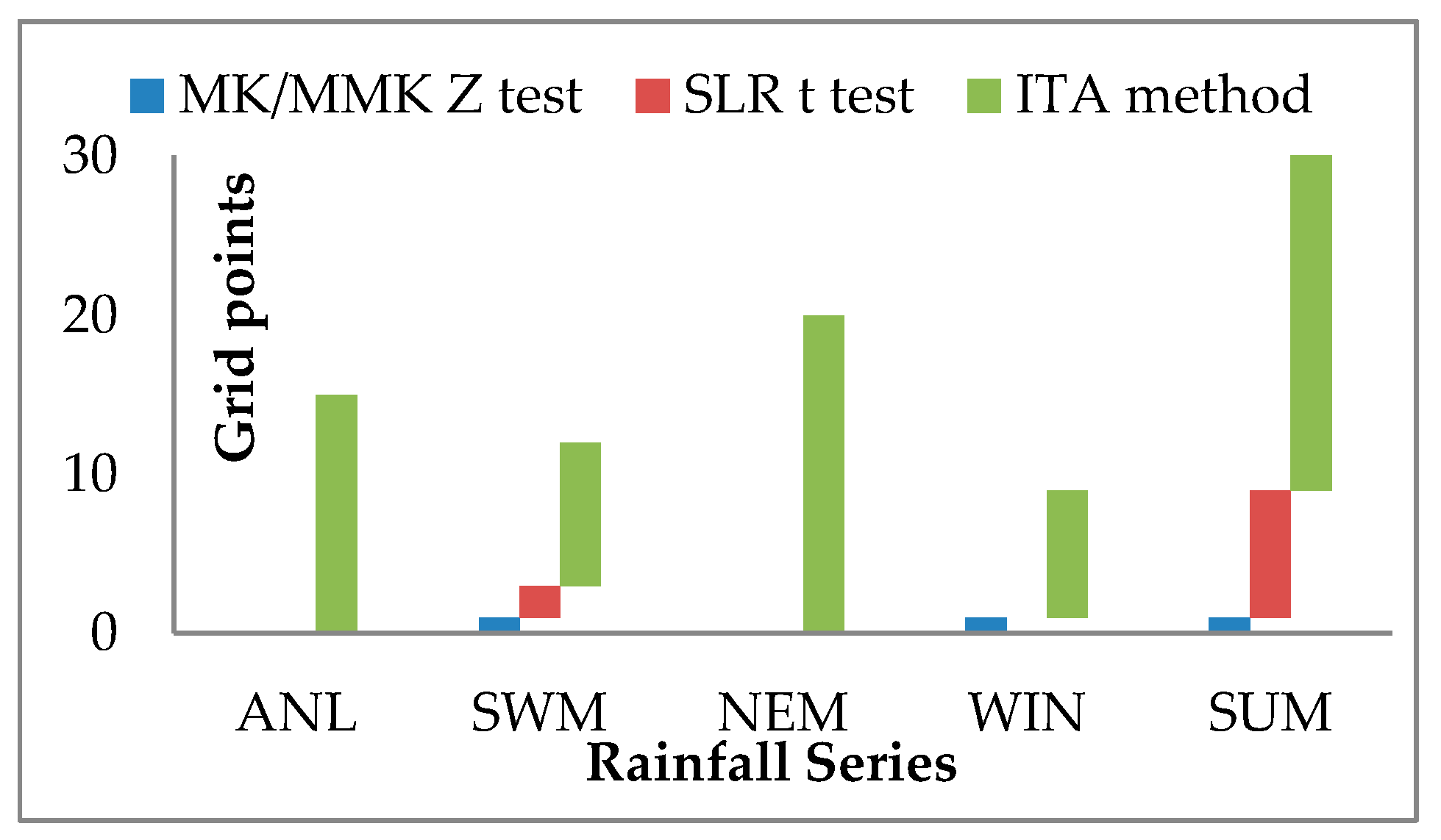
3.9. Comparison of Trend Methods

The number of grid points that exhibited a significant upward or downward trend in seasonal and annual rainfall series is displayed in Figure 7. A total of 130 rainfall series, including annual and four seasonal series, were analyzed for trends in 26 grid points using the SLR, MK/MMK, and ITA methods. The test results were compared based on the number of significant upward or downward trends identified.

Among the three methods used, namely SLR, MK/MMK, and ITA, significant trends were observed in 2.3%, 7.7%, and 44.6% of the grid points, respectively. Notably, the SLR and MK/MMK methods detected significant trends only in the SWM, winter, and summer series, while no trends were identified in the annual and NEM series. It is noteworthy that SLR and MK/MMK methods only identified significant trends in the SWM, winter, and summer series, while they did not detect trends in the annual and NEM series. It is worth mentioning that all ten significant trends detected by the SLR test were also identified by the ITA method. However, the significant trend detected by the MK test did not align with the ITA method. One significant trend identified by the MMK method was also detected by the ITA method.

Table 8. Correlation between the test statistics of MK and SLR with the slope values.

	ANL		SWM		NEM		WIN		SUM
	MKT	SLR	MKT	SLR	MKT	SLR	MKT	SLR	MKT	SLR
ITA	0.896	0.828	0.692	0.851	0.359	0.335	0.461	0.969	0.937	0.958
MKT	1.00	0.841	1.00	0.803	1.00	0.887	1.00	0.592	1.00	0.948

presents the correlation between the test statistics of the MK and SLR methods with the slope values of the ITA method, regardless of the level of significance. It was observed that the MK test showed good correlation with the ITA method in the annual and summer series. Similarly, the correlation between the SLR test and the ITA method was found to be good for the annual, SWM, winter, and summer series.

The study findings suggest that the ITA method outperforms traditional trend detection methods. The ITA method proved beneficial in detecting many significant trends that could not be identified by the traditional methods in the annual and seasonal rainfall series. It effectively revealed hidden trends in rainfall series across the grid points. Many researchers have validated the Sen’s (2012) [8] ITA methodology for different hydro-meteorological variables in various parts of the world [4,14,17,50,89,104,105,106,107,108,109,110]. Unlike classical methods, the ITA method does not require prewhitening prior to its application [8]. Trends of low, medium, and high data can be easily observed using this method [99,111]. One disadvantage of this test is that it must be applied to each recorded series individually [112]. The possibility of presenting results graphically in this method enables the easy observation of hidden subtrends and helps in identifying trends in extreme values [63,113].

The findings of the present study indicate that a majority of the grid points in the western and eastern parts of the Vaippar basin show a significant increasing trend in rainfall. This increasing trend is significant as it can contribute to an increase in runoff, which can be utilized for water management purposes, particularly for tapping and harnessing the runoff water in addition to the existing water conservation structures.

Conversely, it was also observed that some grid points exhibit a significant downward trend in rainfall. This decline in rainfall presents various challenges and implications for surface and groundwater management. One of the key challenges is the increased reliance on groundwater extraction for crop irrigation, leading to the depletion of groundwater reserves, drought-related issues, and diminished soil moisture [44].

Given these observations, it is crucial to carefully consider the changes in rainfall patterns and trends in long-term catchment-scale water management strategies. Adapting and planning for these changes can help mitigate the potential risks associated with declining precipitation, such as implementing measures to enhance water conservation, exploring alternative water sources, and promoting sustainable agricultural practices that optimize water usage. Long-term water management strategies should take into account the evolving rainfall patterns to ensure efficient and sustainable utilization of water resources in the Vaippar basin.

4. Conclusions

This study aimed to analyze the variation and trends of seasonal and annual rainfall series in the Vaippar basin using gridded rainfall data from 1971 to 2019. The SLR, MK/MMK, and ITA methods were employed to examine the trends, magnitudes, subtrends, and nature of the trend. In order to account for spatial variability, monthly rainfall data from 13 rain gauge stations within the basin were spatially interpolated using the inverse distance weighing (IDW) method under GIS environment. To further refine the spatial representation, the basin was divided into 26 grids, each covering approximately 205 km², and gridded rainfall data was generated from the interpolated gauge data. The key findings and conclusions of this study are summarized below.

The basin experienced moderate variability in annual rainfall, lower variability during the NEM season, and higher variability in other seasons. Among the three methods (SLR, MK/MMK, and ITA), significant trends were detected in 2.3%, 7.7%, and 44.6% of the grid points, respectively. The SLR and MK/MMK methods detected significant trends only in the SWM, winter, and summer series. The significant trend detected by the MK test did not align with the ITA method, but the significant trends detected by the SLR test were consistent with the ITA method. The ITA method indicated that 57.69%, 76.92%, and 80.77% of the grid points exhibited significant trends at 5% and 10% significance levels in annual, NEM, and summer rainfall, respectively. However, the SWM and winter series showed less than 35% significant trends. For the NEM season, 53.85% of the grids displayed a significant upward trend, which is a positive sign for improving water management. Grid points located in the southwestern and central parts of the basin showed a higher number of significant trends in annual rainfall. In terms of the NEM season, the southeastern, central, and extreme southern parts experienced a significant upward trend.

In the annual and NEM series, grid points located in the southwestern parts of the basin exhibited monotonically upward trends. Approximately 19.3% of the grid points in the southwestern parts of the basin showed upward trends in high rainfall segments, as classified for annual and NEM rainfall. Grid points in the western part of the basin exhibited a significantly upward trend with a slope of 2.03 mm/year, while the central part showed a non-significant downward trend with a slope value of −1.89 mm/year for the NEM series. Among the three methods considered, the ITA method consistently estimated a higher magnitude of trend for all the rainfall series compared to the other methods. Compared with traditional methods, the ITA method, which represents rainfall series graphically without making any assumptions, detected trends that were not identified by traditional methods. It facilitated the identification of monotonic or non-monotonic upward/downward trends and trends in low, medium, and high rainfall segments.

From the spatial analysis of the Vaippar basin, it is evident that the southeastern, central, and extreme southern parts have exhibited a positive increase in annual rainfall. Moreover, when considering different seasons, it is notable that the NEM season has displayed widespread positive trends across various parts of the basin. These positive rainfall trends have significant implications for water availability, agricultural productivity, and overall ecological balance within the Vaippar basin. The significant findings of this study will serve as a crucial scientific reference for policymakers, assisting in the preparation and management of extreme climate effects on land and water resources within and around the Vaipaar basin.

References

1. FAO. India at a Glance. FAO in India. Available online: https://www.fao.org/india/fao-in-india/india-at-a-glance/en/ (accessed on 22 July 2023).
2. TNENVIS. Agriculture. Available online: http://tnenvis.nic.in/Database/TN-ENVIS_792.aspx (accessed on 27 July 2023).
3. Kumaraperumal, R.; Pazhanivelan, S.; Ragunath, K.P.; Raman, M.G. Mapping of rainfed areas in Tamil Nadu using Remote Sensing Technology. Madras Agric. J. 2019, 106, 643. [Google Scholar]
4. Wang, Y.; Xu, Y.; Tabari, H.; Wangb, J.; Wangb, Q.; Songd, S.; Hu, Z. Innovative trend analysis of annual and seasonal rainfall in the Yangtze River Delta, eastern China. Atmos. Res. 2020, 231, 104673. [Google Scholar] [CrossRef]
5. IPCC (Intergovernmental Panel on Climate Change). Summary for policymakers. In Global Warming of 1.5 °C—An IPCC Special Report on the Impacts of Global Warming of 1.5 °C above Pre-Industrial Levels and Related Global Greenhouse Gas Emission Pathways, in the Context of Strengthening the Global Response to World Meteorol; Organ: Geneva, Switzerland, 2018; Volume 106, p. 32. [Google Scholar]
6. Mishra, A.K.; Singh, V.P. A review of drought concepts. J. Hydrol. 2010, 391, 202–216. [Google Scholar] [CrossRef]
7. Sun, F.; Roderick, M.L.; Farquhar, G.D. Rainfall statistics, stationarity, and climate change. Proc. Natl. Acad. Sci. USA 2018, 115, 2305–2310. [Google Scholar] [CrossRef]
8. Sen, Z. Innovative trend analysis methodology. J. Hydrol. Eng. 2012, 17, 1042–1046. [Google Scholar] [CrossRef]
9. Mondal, A.; Khare, D.; Kundu, S. Spatial and temporal analysis of rainfall and temperature trend of India. Theor. Appl. Clim. 2015, 122, 143–158. [Google Scholar] [CrossRef]
10. Ahmadi, F.; Tahroudi, M.N.; Mirabbasi, R.; Khalili, K.; Jhajharia, D. Spatiotemporal trend and abrupt change analysis of temperature in Iran. Meteorol. Appl. 2017, 25, 314–332. [Google Scholar] [CrossRef]
11. Machiwal, D.; Jha, M.K. Hydrologic Time Series Analysis: Theory and Practice, 1st ed.; Springer: Berlin/Heidelberg, Germany; Capital Publishing Company: New Delhi, India, 2012. [Google Scholar]
12. Machiwal, D.; Jha, M.K. Evaluating persistence and identifying trends and abrupt changes in monthly and annual rainfalls of a semi-arid region in Western India. Theor. Appl. Clim. 2017, 128, 689–708. [Google Scholar] [CrossRef]
13. Kumar, S.; Machiwal, D.; Dayal, D. Spatial modelling of rainfall trends using satellite datasets and geographic information system. Hydrol. Sci. J. 2017, 62, 1636–1653. [Google Scholar] [CrossRef]
14. Machiwal, D.; Gupta, A.; Jha, M.K.; Kamble, T. Analysis of trend in temperature and rainfall time series of an Indian arid region: Comparative evaluation of salient techniques. Theor. Appl. Clim. 2018, 136, 301–320. [Google Scholar] [CrossRef]
15. Malik, A.; Kumar, A. Spatio-temporal trend analysis of rainfall using parametric and non-parametric tests: Case study in Uttarakhand, India. Theor. Appl. Clim. 2020, 140, 183–207. [Google Scholar] [CrossRef]
16. Tabari, H.; Marofi, S.; Ahmadi, M. Long-term variations of waterquality parameters in the Maroon River Iran. Environ. Monit. Assess. 2010, 177, 273–287. [Google Scholar] [CrossRef]
17. Singh, R.; Sah, S.; Das, B.; Potekar, S.; Chaudhary, A.; Pathak, H. Innovative trend analysis of spatio-temporal variations of rainfall in India during 1901–2019. Theor. Appl. Clim. 2021, 145, 821–838. [Google Scholar] [CrossRef]
18. Hirsch, R.M.; Alexander, R.B.; Smith, R.A. Selection of methods for the detection and estimation of trends in water quality. Water Resour. Res. 1971, 27, 803–813. [Google Scholar] [CrossRef]
19. Ahmad, T.; Pandey, A.C.; Kumar, A. Long-term precipitation monitoring and its linkage with flood scenario in changing climate conditions in Kashmir valley. Geocarto Int. 2021, 37, 5497–5522. [Google Scholar] [CrossRef]
20. Singh, R.; Sah, S.; Das, B.; Vishnoi, L.; Pathak, H. Spatio-temporal trends and variability of rainfall in Maharashtra, India: Analysis of 118 years. Theor. Appl. Clim. 2020, 143, 883–900. [Google Scholar] [CrossRef]
21. Kumar, S.; Merwade, V.; Kam, J.; Thurner, K. Streamflow trends in Indiana: Effects of long term persistence, precipitation and subsurface drains. J. Hydrol. 2009, 374, 171–183. [Google Scholar] [CrossRef]
22. Zamani, R.; Mirabbasi, R.; Abdollahi, S.; Jhajharia, D. Streamflow trend analysis by considering autocorrelation structure, long-term persistence and Hurst coefficient in a semi-arid region of Iran. Theor. Appl. Clim. 2017, 129, 33–45. [Google Scholar] [CrossRef]
23. Dinpashoh, Y.; Mirabbasi, R.; Jhajharia, D.; Abianeh, H.Z.; Mostafaeipour, A. Effect of short-term and long-term persistence on identification of temporal trends. J. Hydrol. Eng. 2014, 19, 617–625. [Google Scholar] [CrossRef]
24. Sonali, P.; Kumar, D.N. Spatio-temporal variability of temperature and potential evapotranspiration over India. J. Water Clim. Change 2016, 7, 810–822. [Google Scholar] [CrossRef]
25. Amirataee, B.; Montaseri, M.; Sanikhani, H. The analysis of trend variations of reference evapotranspiration via eliminating the significance effect of all autocorrelation coefficients. Theor. Appl. Clim. 2016, 126, 131–139. [Google Scholar] [CrossRef]
26. Praveenkumar, C.; Jothiprakash, V. Spatio-temporal trend and homogeneity analysis of gridded and gauge precipitation in Indravati river basin, India. J. Water Clim. Change 2018, 11, 178–199. [Google Scholar] [CrossRef]
27. Kumar, M.S.; Geethalakshmi, V.; Ramanathan, S.; Senthil, A.; Senthilraja, K.; Bhuvaneswari, K.; Gowtham, R.; Kannan, B.; Priyanka, S. Rainfall Spatial-Temporal Variability and Trends in the Thamirabharani River Basin, India: Implications for Agricultural Planning and Water Management. Sustainability 2022, 14, 14948. [Google Scholar] [CrossRef]
28. Krishnakumar, K.N.; Rao, G.S.L.H.V.P.; Gopakumar, C.S. Rainfall trends in twentieth century over Kerala, India. Atmos. Environ. 2009, 43, 1940–1944. [Google Scholar] [CrossRef]
29. Kumar, V.; Jain, S. Rainfall trend in Ganga-Brahmputra-Meghna river basins of India (1951–2004). J. Hydrol. 2010, 33, 59–66. [Google Scholar]
30. Manikandan, M.; Tamilmani, D. Statistical Analysis of Spatial Pattern of Rainfall Trends in Parambikualam-Aliyar Sub Basin, Tamil Nadu. J. Indian Water Resour. Soc. 2012, 32, 40–49. [Google Scholar]
31. Suryavanshi, S.; Pandey, A.; Chaube, U.C.; Joshi, N. Long-term historic changes in climatic variables of Betwa Basin, India. Theor. Appl. Clim. 2014, 117, 403–418. [Google Scholar] [CrossRef]
32. Jhajharia, D.; Dinpashoh, Y.; Kahya, E. Trends in temperature over Godavari River basin in Southern Peninsular India. Int. J. Clim. 2014, 34, 1369–1384. [Google Scholar] [CrossRef]
33. Taxak, A.K.; Murumkar, A.R.; Arya, D.S. Long term spatial and temporal rainfall trends and homogeneity analysis in Wainganga basin, Central India. Weather Clim. Extrem. 2014, 4, 50–61. [Google Scholar] [CrossRef]
34. Gajbhiye, S.; Meshram, C.; Mirabbasi, R.; Sharma, S.K. Trend analysis of rainfall time series for Sindh river basin in India. Theor. Appl. Clim. 2015, 125, 593–608. [Google Scholar] [CrossRef]
35. Raju, B.C.K.; Nandagiri, L. Analysis of historical trends in hydrometeorological variables in the upper Cauvery Basin, Karnataka, India. Curr. Sci. 2017, 112, 577–587. [Google Scholar] [CrossRef]
36. Anand, B.; Karunanidhi, D. Long term spatial and temporal rainfall trend analysis using GIS and statistical methods in Lower Bhavani basin, Tamil Nadu, India. Indian J. Geo-Mar. Sci. 2020, 49, 419–427. [Google Scholar]
37. Bisht, D.S.; Chatterjee, C.; Raghuwanshi, N.S.; Sridhar, V. Spatiotemporal trends of rainfall across Indian river basins. Theor. Appl. Clim. 2018, 132, 419–436. [Google Scholar] [CrossRef]
38. Chandniha, S.K.; Meshram, S.G.; Adamowski, J.F.; Meshram, C. Trend analysis of precipitation in Jharkhand State, India. Theor. Appl. Clim. 2016, 130, 261–274. [Google Scholar] [CrossRef]
39. Sharma, S.; Singh, P.K. Long Term Spatiotemporal Variability in Rainfall Trends over the State of Jharkhand, India. Climate 2017, 5, 18. [Google Scholar] [CrossRef]
40. Meshram, S.G.; Singh, V.P.; Meshram, C. Long-term trend and variability of precipitation in Chhattisgarh State. India. Theor. Appl. Clim. 2016, 129, 729–744. [Google Scholar] [CrossRef]
41. Gajbhiye, S.; Meshram, C.; Singh, S.K.; Srivastava, P.K.; Islam, T. Precipitation trend analysis of Sindh River basin, India, from 102-year record (1901–2002). Atmos. Sci. Lett. 2016, 17, 71–77. [Google Scholar] [CrossRef]
42. Dhorde, A.G.; Korade, M.S.; Dhorde, A.A. Spatial distribution of temperature trends and extremes over Maharashtra and Karnataka states of India. Theor. Appl. Clim. 2017, 130, 191–204. [Google Scholar] [CrossRef]
43. Machiwal, D.; Kumar, S.; Dayal, D. Characterizing rainfall of hot arid region by using time-series modelling and sustainability approaches: A case study from Gujarat, India. Theor. Appl. Clim. 2016, 124, 593–607. [Google Scholar] [CrossRef]
44. Sanikhani, H.; Kisi, O.; Mirabbasi, R.; Meshram, S.G. Trend analysis of rainfall pattern over the Central India during 1901–2010. Arab. J. Geosci. 2018, 11, 437. [Google Scholar] [CrossRef]
45. Pingale, S.M.; Khare, D.; Jat, M.K.; Adamowski, J. Spatial and temporal trends of mean and extreme rainfall and temperature for the 33 urban centers of the arid and semi-arid state of Rajasthan, India. Atmos. Res. 2014, 138, 73–90. [Google Scholar] [CrossRef]
46. Pingale, S.M.; Khare, D.; Jat, M.K.; Adamowski, J. Trend analysis of climatic variables in an arid and semi-arid region of the Ajmer District, Rajasthan, India. J. Water Land Dev. 2016, 28, 3–18. [Google Scholar] [CrossRef]
47. Meena, H.M.; Machiwal, D.; Santra, P.; Moharana, P.C.; Singh, D.V. Trends and homogeneity of monthly, seasonal, and annual rainfall over arid region of Rajasthan, India. Theor. Appl. Clim. 2018, 136, 795–811. [Google Scholar] [CrossRef]
48. Panda, A.; Sahu, N. Trend analysis of seasonal rainfall and temperature pattern in Kalahandi, Bolangir and Koraput districts of Odisha, India. Atmos. Sci. Lett. 2019, 20, e932. [Google Scholar] [CrossRef]
49. Patakamuri, S.K.; Muthiah, K.; Sridhar, V. Long-term homogeneity, trend, and change-point analysis of rainfall in the arid district of Ananthapuramu, Andhra Pradesh State, India. Water 2020, 12, 211. [Google Scholar] [CrossRef]
50. Gujree, I.; Ahmad, I.; Zhang, F.; Arshad, A. Innovative Trend Analysis of High-Altitude Climatology of Kashmir Valley, North-West Himalayas. Atmosphere 2022, 13, 764. [Google Scholar] [CrossRef]
51. Wagesho, N.; Goel, N.K.; Jain, M.K. Temporal and spatial variability of annual and seasonal rainfall over Ethiopia. Hydrol. Sci. J. 2013, 58, 354–373. [Google Scholar] [CrossRef]
52. Ay, M.; Kisi, O. Investigation of trend analysis of monthly total precipitation by an innovative method. Theor. Appl. Clim. 2014, 120, 617–629. [Google Scholar] [CrossRef]
53. Manzanas, R.; Amekudzi, L.K.; Preko, K.; Herrera, S.; Guti’errez, J.M. Precipitation variability and trends in Ghana: An intercomparison of observational and reanalysis products. Clim. Change 2014, 124, 805–819. [Google Scholar] [CrossRef]
54. Daniels, E.E.; Lenderink, G.; Hutjes, R.W.A.; Holtslag, A.A.M. Spatial precipitation patterns and trends in The Netherlands during 1951–2009. Int. J. Clim. 2014, 34, 1773–1784. [Google Scholar] [CrossRef]
55. Farhangi, M.; Kholghi, M.; Chavoshian, S.A. Rainfall Trend Analysis of Hydrological Subbasins in Western Iran. J. Irrig. Drain. Eng. 2016, 142, 05016004. [Google Scholar] [CrossRef]
56. Minaei, M.; Irannezhad, M. Spatio-temporal trend analysis of precipitation, temperature, and river discharge in the northeast of Iran in recent decades. Theor. Appl. Clim. 2016, 131, 167–179. [Google Scholar] [CrossRef]
57. Lionello, P.; Abrantes, F.; Gacic, M.; Planton, S.; Trigo, R.; Ulbrich, U. The climate of the Mediterranean region: Research progress and climate change impacts. Reg. Environ. Change 2014, 14, 1679–1684. [Google Scholar] [CrossRef]
58. Valdes-Abellan, J.; Pardoand, M.A.; Tenza-Abril, A.J. Observed Precipitation Trend Changes in the Western Mediterranean Region. Int. J. Clim. 2017, 37, 1285–1296. [Google Scholar] [CrossRef]
59. Kabanda, T. Long-term rainfall trends over the Tanzania coast. Atmosphere 2018, 9, 155. [Google Scholar] [CrossRef]
60. Huang, J.; Sun, S.; Xue, Y.; Zhang, J. Spatial and temporal variability of precipitation indices during 1961–2010 in Hunan Province, central south China. Theor. Appl. Clim. 2014, 118, 581–595. [Google Scholar] [CrossRef]
61. Ye, J.S. Trend and variability of China’s summer precipitation during 1955–2008. Int. J. Clim. 2014, 34, 59–566. [Google Scholar] [CrossRef]
62. Zhang, Y.; Xia, J.; She, D. Spatiotemporal variation and statistical characteristic of extreme precipitation in the middle reaches of the Yellow River Basin during 1960–2013. Theor. Appl. Clim. 2018, 135, 391–408. [Google Scholar] [CrossRef]
63. Wu, H.; Qian, H. Innovative trend analysis of annual and seasonal rainfall and extreme values in Shaanxi, China, since the 1950s. Int. J. Clim. 2017, 37, 2582–2592. [Google Scholar] [CrossRef]
64. Qin, Z.; Peng, D.; Singh, V.P.; Chen, M. Spatio-temporal variations of precipitation extremes in Hanjiang River Basin, China, during 1960–2015. Theor. Appl. Clim. 2019, 138, 1767–1783. [Google Scholar] [CrossRef]
65. Gado, T.A.; El-Hagrsy, R.M.; Rashwa, I.M.H. Spatial and Temporal Rainfall Changes in Egypt. Environ. Sci. Pollut. Res. 2019, 26, 28228–28242. [Google Scholar] [CrossRef]
66. Chattopadhyay, S.D.; Edwards, R.M. Long-term trend analysis of precipitation and air temperature for Kentucky, United States. Climate 2016, 4, 10. [Google Scholar] [CrossRef]
67. Chakraborty, S.; Pandey, R.; Chaube, U.; Mishra, S. Trend and variability analysis of rainfall series at Seonath River Basin, Chhattisgarh (India). Int. J. Appl. Sci. Eng. 2013, 2, 425–434. [Google Scholar]
68. Chandrakar, A.; Khare, D.; Krishan, R. Assessment of Spatial and Temporal Trends of Long Term Precipitation over Kharun Watershed, Chhattisgarh, India. Environ. Process. 2017, 4, 959–974. [Google Scholar] [CrossRef]
69. Sen, Z. Trend identification simulation and application. J. Hydrol. Eng. 2014, 19, 635–642. [Google Scholar] [CrossRef]
70. Tosunoglu, F.; Kisi, O. Trend analysis of maximum hydrologicdrought variables using Mann–Kendall andŞen’s innovative trend method. River Res. Appl. 2017, 33, 597–610. [Google Scholar] [CrossRef]
71. CGWB (Central Ground Water Board). Report on Aquifer Mapping and Management of Ground Water Resources for Viappar Aquifer System Tamil Nadu. Department of Water Resources, River Development and Ganga Rejuvenation, Ministry of Jal Shakti, Government of India. Available online: http://cgwb.gov.in/sites/default/files/2022-1/vaippar_aquifer_system_tn.pdf (accessed on 27 July 2023).
72. Season and Crop Report of Tamilnadu, 2020–21. Department of Economics and Statistics: Chennai, India. Available online: https://agritech.tnau.ac.in/pdf/season%20n%20crop%202021.pdf (accessed on 27 July 2023).
73. Kim, T.; Valdes, J.B.; Aparicio, J. Frequency and spatial characteristics of droughts in the Conchos River Basin, Mexico. Water Int. 2002, 27, 420–430. [Google Scholar] [CrossRef]
74. Edossa, D.C.; Babel, M.S.; Gupta, A.D. Drought analysis in the Awash River Basin, Ethiopia. Water Resour. Manag. 2010, 24, 1441–1460. [Google Scholar] [CrossRef]
75. Moradi, H.R.; Rajabi, M.; Faragzadeh, M. Investigation of meteorological drought characteristics in Fars province, Iran. Catena 2011, 84, 35–46. [Google Scholar] [CrossRef]
76. Mishra, A.K.; Desai, V.R. Drought forecasting using stochastic models. Stoch. Environ. Res. Risk Assess. 2005, 19, 326–339. [Google Scholar] [CrossRef]
77. Shepard, D. A Two-Dimensional Interpolation Function for Irregularly Data. In Proceedings of the 23rd ACM National Conference, Las Vegas, NV, USA, 27–29 August 1968; pp. 517–524. [Google Scholar]
78. Rase, W.D. Volume Preserving Interpolation of a Smooth Surface from Polygon Related Data. J. Geogr. Syst. 2001, 3, 199–213. [Google Scholar] [CrossRef]
79. Mishra, A.K.; Desai, V.R. Spatial and temporal drought analysis in the Kansabati River Basin, India. Int. J. River Basin Manag. 2005, 3, 31–41. [Google Scholar] [CrossRef]
80. Manikandan, M.; Tamilmani, D. Spatial and Temporal Variation of Meteorological Drought in the Parambikulam-Aliyar Basin, Tamil Nadu. J. Inst. Eng. Ser. A 2015, 96, 177–184. [Google Scholar] [CrossRef]
81. Asfaw, A.; Simane, B.; Hassen, A.; Bantider, A. Variability and time series trend analysis of rainfall and temperature in north central Ethiopia: A case study in Woleka sub-basin. Weather Clim. Extrem. 2018, 19, 29–41. [Google Scholar] [CrossRef]
82. Hare, W. Assessment of Knowledge on Impacts of Climate Change, Contribution to the Specification of Art, 2 of the UNFCCC; WBGU: Bowling Green, OH, USA, 2003. [Google Scholar]
83. Gadgil, A.; Dhorde, A. Temperature trends in twentieth century at Pune. India. Atmos. Environ. 2005, 39, 6550–6556. [Google Scholar] [CrossRef]
84. Hameed, T.; Marino, M.A.; DeVries, J.J.; Tracy, J.C. Method for trend detection in climatological variables. J. Hydrol. Eng. 1997, 2, 157–160. [Google Scholar] [CrossRef]
85. Jaiswal, R.K.; Lohani, A.K.; Tiwari, H.L. Statistical analysis for change detection and trend assessment in climatological parameters. Environ. Process. 2015, 2, 729–749. [Google Scholar] [CrossRef]
86. Mann, H.B. Non-parametric tests against trend. Econometrica 1945, 13, 245–259. [Google Scholar] [CrossRef]
87. Kendall, M.G. Rank Correlation Methods; Charles Griffin and Co., Ltd.: London, UK, 1975. [Google Scholar]
88. Sonali, P.; Kumar, D.N. Review of trend detection methods and their application to detect temperature changes in India. J. Hydrol. 2013, 476, 212–227. [Google Scholar] [CrossRef]
89. Malik, A.; Kumar, A.; Guhathakurta, P.; Kisi, O. Spatial-temporal trend analysis of seasonal and annual rainfall (1966–2015) using innovative trend analysis method with significance test. Arab. J. Geosci. 2019, 12, 10. [Google Scholar] [CrossRef]
90. Hamed, K.H.; Rao, A.R. A modified Mann-Kendall trend test for auto correlated data. J. Hydrol. 1998, 204, 182–196. [Google Scholar] [CrossRef]
91. Modarres, R.; Silva, V.P.R. Rainfall trends in arid and semi-arid regions of Iran. J. Arid Environ. 2007, 70, 344–355. [Google Scholar] [CrossRef]
92. Yue, S.; Pilon, P.; Phinney, B. Canadian streamflow trend detection: Impacts of serial and cross-correlation. Hydrol. Sci. J. 2003, 48, 51–63. [Google Scholar] [CrossRef]
93. Novotny, E.V.; Stefan, H.G. Stream flow in Minnesota: Indicator of Climate Change. J. Hydrol. 2007, 334, 319–333. [Google Scholar] [CrossRef]
94. Rai, R.K.; Upadhyay, A.; Ojha, C.S.P. Temporal variability of climatic parameters of Yamuna River Basin: Spatial analysis of persistence, trend and periodicity. Open Hydrol. J. 2010, 4, 184–210. [Google Scholar] [CrossRef]
95. Luo, Y.; Lio, S.; Sheng, L.; Fu, S.; Liu, J.; Wang, G.; Zhou, G. Trends of precipitation in Beijiang River Basin, Guangdong Province, China. Hydrol. Process. 2008, 22, 2377–2386. [Google Scholar] [CrossRef]
96. Karpouzos, D.K.; Kavalieratou, S.; Babajimopoulos, C. Trend analysis of precipitation data in Pieria region (Greece). Eur. Water 2010, 30, 31–40. [Google Scholar]
97. Anderson, R.L. Distribution of the serial correlation coefficient. Ann. Math. Stat. 1942, 13, 1–13. [Google Scholar] [CrossRef]
98. Sen, P.K. Estimates of the regression coefficient based on Kendall’s tau. J. Am. Stat. Assoc. 1968, 63, 1379–1389. [Google Scholar] [CrossRef]
99. Kisi, O. An innovative method for trend analysis of monthly pan evaporations. J. Hydrol. 2015, 527, 1123–1129. [Google Scholar] [CrossRef]
100. Tabari, H.; Willems, P. Investigation of streamflow variation using an innovative trend analysis approach in Northwest Iran. In Proceedings of the 36th IAHR World Congress, The Hague, The Netherlands, 28 June–3 July 2015. [Google Scholar]
101. Sen, Z. Innovative trend significance test and applications. Theor. Appl. Clim. 2017, 127, 939–947. [Google Scholar] [CrossRef]
102. Yue, S.; Hashino, M. Long term trends of annual and monthly precipitation in Japan. J. Am. Water Resour. Assoc. 2003, 39, 587–596. [Google Scholar] [CrossRef]
103. Some’e, B.S.; Ezani, A.; Tabari, H. Spatiotemporal trends and change point of precipitation in Iran. Atmos. Res. 2012, 113, 1–12. [Google Scholar]
104. Caloiero, T.; Coscarelli, R.; Ferrari, E. Application of the Innovative Trend Analysis Method for the Trend Analysis of Rainfall Anomalies in Southern Italy. Water Resour. Manag. 2018, 32, 4971–4983. [Google Scholar] [CrossRef]
105. Güçlü, Y.S. Improved visualisation for trend analysis by comparing with classical Mann-Kendall test and ITA. J. Hydrol. 2020, 584, 124674. [Google Scholar] [CrossRef]
106. Marak, J.D.K.; Sarma, A.K.; Bhattacharjya, R.K. Innovative trend analysis of spatial and temporal rainfall variations in Umiam and Umtru watersheds in Meghalaya, India. Theor. Appl. Clim. 2020, 142, 1397–1412. [Google Scholar] [CrossRef]
107. Dong, Z.; Jia, W.; Sarukkalige, R.; Fu, G.; Meng, Q.; Wang, Q. Innovative Trend Analysis of Air Temperature and Precipitation in the Jinsha River Basin, China. Water 2020, 12, 3293. [Google Scholar] [CrossRef]
108. Ahmed, I.A.; Salam, R.; Naikoo, M.W.; Rahman, A.; Praveen, B.; Hoai, P.N.; Pham, Q.B.; DuongAnh, T.; Tri, D.Q.; Elkhrachy, I. Evaluating the variability in long-term rainfall over India with advanced statistical techniques. Acta Geophys. 2022, 70, 801–818. [Google Scholar] [CrossRef]
109. Chauhan, A.S.; Maurya, R.K.S.; Rani, A.; Malik, A.; Kisi, O.; Danodia, A. Rainfall dynamics observed over India during last century (1901–2020) using innovative trend methodology. Water Supply 2022, 22, 6909–6944. [Google Scholar] [CrossRef]
110. Alashan, S. Comparison of sub-series with different lengths using şen-innovative trend analysis. Acta Geophys. 2023, 71, 373–383. [Google Scholar] [CrossRef]
111. Katipoğlu, O.M. Analyzing the trend and change point in various meteorological variables in Bursa with various statistical and graphical methods. Theor. Appl. Clim. 2022, 150, 1295–1320. [Google Scholar] [CrossRef]
112. Haktanir, T.; Citakoglu, H. Trend, independence, stationarity, and homogeneity tests on maximum rainfall series of standard durations recorded in Turkey. J. Hydrol. Eng. 2014, 19, 9. [Google Scholar] [CrossRef]
113. Madane, D.A.; Waghaye, A.M. Spatio-temporal variations of rainfall using innovative trend analysis during 1951–2021 in Punjab State, India. Theor. Appl. Clim. 2023, 153, 923–945. [Google Scholar] [CrossRef]
Figure 1. Geographical location of study area along with (a) rain gauge stations and (b) grid points in subbasin.
Sustainability 16 01957 g001
Figure 2. The overall process involved for rainfall characterization.
Sustainability 16 01957 g002
Figure 3. Test results of Simple Linear Regression (SLR) at 5 and 10% significance level for (a) annual (ANL), (b) southwest monsoon (SWM) (c) northeast monsoon (NEM), (d) winter (WIN), (e) summer (SUM) gridded rainfall series of Vaippar basin.
Sustainability 16 01957 g003aSustainability 16 01957 g003b
Figure 4. Autocorrelation coefficient at lag-1 period for annual and seasonal rainfall series of Vaippar basin. (ANL—annual, SWM—southwest monsoon, NEM—northeast monsoon, WIN—winter, SUM—summer).
Sustainability 16 01957 g004
Figure 5. Mann–Kendall and Modified Mann–Kendall Z values at 5 and 10% significance level for (a) annual (ANL), (b) southwest monsoon (SWM) (c) northeast monsoon (NEM), (d) winter (WIN), (e) summer (SUM) gridded rainfall series of Vaippar basin.
Sustainability 16 01957 g005
Figure 6. The ITA slope values at 5 and 10% significance level for (a) annual (ANL), (b) southwest monsoon (SWM) (c) northeast monsoon (NEM), (d) winter (WIN), (e) summer (SUM) gridded rainfall series of Vaippar basin.
Sustainability 16 01957 g006aSustainability 16 01957 g006b
Figure 7. Grid points exhibited significant trend in Monthly, Seasonal and Annual rainfall series.
Sustainability 16 01957 g007