Urban Traffic Flow Prediction Based on Bayesian Deep Learning Considering Optimal Aggregation Time Interval

Abstract

Predicting short-term urban traffic flow is a fundamental and cost-effective strategy in traffic signal control systems. However, due to the interrupted, periodic, and stochastic characteristics of urban traffic flow influenced by signal control, there are still unresolved issues related to the selection of the optimal aggregation time interval and the quantifiable uncertainties in prediction. To tackle these challenges, this research introduces a method for predicting urban interrupted traffic flow, which is based on Bayesian deep learning and considers the optimal aggregation time interval. Specifically, this method utilizes the cross-validation mean square error (CVMSE) method to obtain the optimal aggregation time interval and to establish the relationship between the optimal aggregation time interval and the signal cycle. A Bayesian LSTM-CNN prediction model, which extends the LSTM-CNN model under the Bayesian framework to a probabilistic model to better capture the stochasticity and variation in the data, is proposed. Experimental results derived from real-world data demonstrate gathering traffic flow data based on the optimal aggregation time interval significantly enhances the prediction accuracy of the urban interrupted traffic flow model. The optimal aggregation time interval for urban interrupted traffic flow data corresponds to a multiple of the traffic signal control cycle. Comparative experiments indicate that the Bayesian LSTM-CNN prediction model outperforms the state-of-the-art prediction models.

1. Introduction

Predicting traffic flow is a crucial aspect of intelligent transportation systems, and real-time, precise traffic flow predictions serve as the foundation for executing traffic management, providing guidance, and mitigating road congestion. In contrast to the continuous traffic flow on highways, urban traffic flow exhibits interrupted, periodic, and stochastic features due to factors like signal control. Consequently, accurately predicting short-term urban traffic flow presents even greater challenges.

Currently, most urban short-term traffic flow prediction often aggregates traffic flow data into fixed statistical interval time series such as 5 min or 10 min, then uses statistical models, machine learning models, and deep learning models to predict traffic flow data in the future. The selection of an optimal aggregation time interval and the quantification of uncertainties in prediction outcomes remain unresolved issues, impeding the development of robust and reliable traffic flow prediction models. Addressing these challenges is crucial for enhancing the effectiveness of traffic signal control systems and ultimately improving urban transportation efficiency and sustainability.

The urban short-term traffic flow prediction models based on statistics mainly include the autoregressive integrated moving average model (ARIMA) [1], Kalman Filter (KF), and Wavelet Kalman Filter (WKF) [2]. For example, Kamarianakis and Prastacos [3] used a Spatiotemporal Autoregressive Moving Average (STARIMA) model to incorporate data from links upstream to the link of interest in their prediction model. The model was found to be adaptable when the traffic flow is unsteady.

Prediction models based on machine learning mainly include the support vector machine (SVM) [4], and K-Nearest Neighbors (KNN) [5] have also been explored because they are well-suited to model the complex spatiotemporal relationships in data. For instance, Asif performed prediction for a large interconnected road network and for multiple prediction horizons with an SVR-based algorithm [4]. Cheng aggregated the traffic flow into a 5 min time interval and proposed an adaptive spatiotemporal k-nearest neighbor model [5].

The prediction model based on deep learning mainly uses recurrent neural networks (RNNs) [6], convolution neural networks (CNNs) [7], and graph convolution neural networks (GCNs) [8] to predict the traffic flow. Zhao used a single Long Short-Term Memory (LSTM) model to predict the traffic flow of 15, 30, 45, and 60 min time periods [6]. Tang put forward a STGGAT model based on the license plate recognition record and integrating the original data into a 5 min time interval [8]. The above models do not consider the impact of the periodicity of intermittent traffic flow data on the aggregation time interval in the statistical processing of original traffic flow data, and directly select one or more fixed aggregation time intervals, which may lead to the statistical fluctuation of intermittent traffic flow time series.

In the processing and prediction of traffic flow data, the choice of an aggregation time interval is an important factor. Some researchers have found that directly choosing one or more fixed aggregation time intervals may lead to statistical fluctuations in the time series of interrupted traffic flow, and may overlook the impact of the periodicity of interrupted flow data on the aggregation time interval. Zellner [9] found through the study of econometric data that time aggregation would lead to lower prediction accuracy, reduce the ability to test and make short-term predictions, and reduce the probability of finding real short-term data anomalies. Rossana [10] studied the impact of time aggregation on data. Through the study of monthly, quarterly, and annual data, it was found that time aggregation caused a large amount of information loss in the process of data aggregation by eliminating low-frequency changes. Vlahogianni [11] found through the study of urban intersection traffic flow data that time aggregation would eliminate the time change characteristics in traffic flow data, leading to the loss of important information, and some linear models such as ARIMA could not capture the time change characteristics in traffic flow data. Therefore, to retain the important information of traffic flow data to the greatest extent, it is necessary to determine the optimal aggregation time interval of data before forecasting, especially when forecasting complex traffic interruption.

Currently, the analysis of optimal aggregation time interval mainly includes the cross validation mean square error method [12], chart-based statistical method [13], and wavelet analysis method [14]. Byron proposed to use a cross-validation mean square error (CVMSE) model to find the optimal aggregation time interval of traffic flow data. The original traffic flow data is aggregated into different time intervals, and the CVMSE of traffic flow is calculated. The aggregation time interval with the smallest CVMSE is considered the optimal aggregation time interval [12]. Yu [15], based on the wavelet decomposition method, obtained the best integration degree of the data through hierarchical and similarity analysis of ITS data, and completed the data integration. Weerasekera [16] investigated the ability of several algorithms to reliably model traffic flow at different data resolutions.

In this context, this research endeavors to introduce a novel approach for predicting urban interrupted traffic flow, leveraging Bayesian deep learning while considering the critical aspect of the optimal aggregation time interval. This paper is a step towards addressing these challenges. We make the following key contributions: Firstly, by introducing the concept of the optimal aggregation time interval based on CVMSE and its relationship with the signal cycle, we provide a novel approach to address the challenges posed by the interrupted, periodic, and stochastic characteristics of urban traffic flow. Secondly, by employing Bayesian deep learning techniques, specifically the Bayesian LSTM-CNN prediction model, we extend the existing LSTM-CNN architecture to a probabilistic model that better captures the inherent stochasticity and variation in the data. Our experimental results, derived from real-world data, demonstrate the significant improvement in prediction accuracy achieved by gathering traffic flow data based on the optimal aggregation time interval. Furthermore, our findings reveal that the optimal aggregation time interval for urban interrupted traffic flow data corresponds to a multiple of the traffic signal control cycle.

In the rest of the paper, Section 2 provides a detailed description of our proposed methodology. In Section 3, we present the experimental setup and evaluation results. Finally, in Section 4, we conclude the paper by summarizing the contributions of our research and discussing avenues for future work.

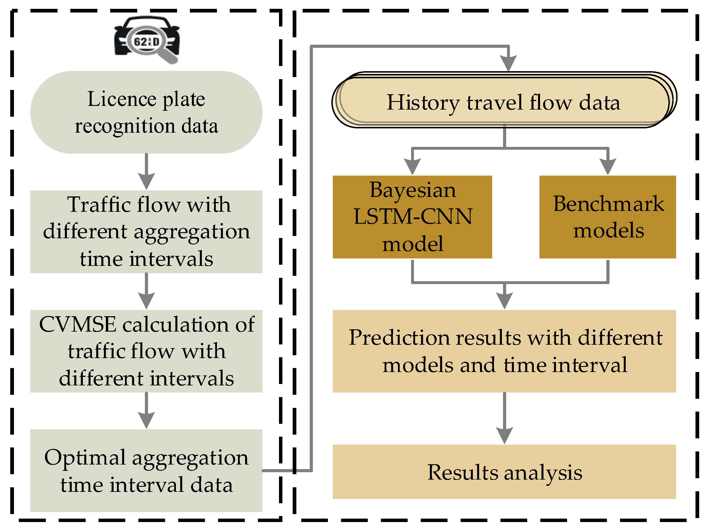
2. Materials and Methods

The methodology proposed by this paper aims to predict urban interrupted traffic flow by leveraging Bayesian deep learning techniques and considering the optimal aggregation time interval.

To determine the optimal aggregation time interval, we utilize a CVMSE model. This model analyzes the performance of different aggregation time intervals and identifies the one that minimizes the error. By considering the optimal aggregation time interval, we can effectively capture the dynamics of traffic flow influenced by signal control and improve the accuracy of our predictions.

Furthermore, to account for the inherent stochasticity and variation in urban traffic flow data, we propose the use of a Bayesian LSTM-CNN prediction model. This model extends the conventional LSTM-CNN architecture by incorporating Bayesian techniques, allowing us to obtain probabilistic predictions. The Bayesian framework enables us to quantify uncertainties associated with the predicted traffic flow, providing valuable insights into the reliability and confidence of the predictions.

In the following sections, we will provide a detailed description of the steps involved in determining the optimal aggregation time interval, developing the Bayesian LSTM-CNN prediction model, and evaluating the performance of our proposed methodology using real-world traffic flow data. The whole framework is shown in Figure 1.

2.1. Problem Definition

Traffic flow prediction aims to predict the future traffic conditions of the road network based on the historical traffic flow data observed. Given the historical data $X=(X_{t_{p-(Q-1)}},\dots ,X_{t_{p-1}},X_{t_p})\in R^{Q\times N}$ of Q time steps on N nodes at time p, it is hoped to predict the traffic conditions of the next R time steps $Y=(X_{t_{p+1}},X_{t_{p+2}},\dots ,X_{t_{p+R}})\in R^{R\times N}$.

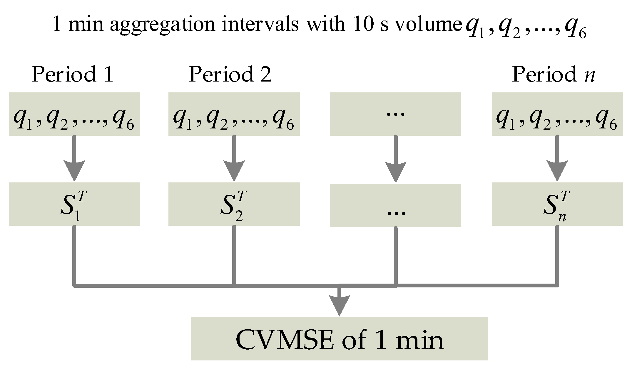
2.2. Optimal Aggregation Time Interval Based on Cross-Validation Mean Square Error

The core concept of determining the optimal aggregation time interval for traffic flow data involves analyzing the dispersion of traffic flow data derived from various aggregation time intervals. Variance serves as the ideal statistical measure for this purpose, hence the frequent use of the CVMSE method. The point at which the CVMSE reaches its minimum signifies the least dispersion and minimal fluctuation in traffic flow. Consequently, the aggregation time interval corresponding to this minimum is deemed the optimal one. This study employs the CVMSE method to investigate the optimal aggregation time interval for urban interrupted traffic flow influenced by traffic control, further analyzing and determining the correlation between the optimal aggregation time interval and the signal cycle.

The basic idea of CVMSE is to take out one value, attempt to predict this value with an aggregated mean, and then take this difference squared and average this for all values within the period of interest, as shown in Figure 2. The specific formula is as follows:

$$S_n^T={\displaystyle \sum _{m=1}^{T/t}{(q_{mn}-\overline{q_n^{(m)}})}^2}.$$

(1)

where $S_n^T$ represents the cross-validation mean square error for the n-th set of data when the time interval for data aggregation is T. $q_{mn}\hspace{0.33em}$ represents the m-th original flow data in the n-th set of data sequence, $\overline{q_n^{(m)}}\hspace{0.33em}$ represents the mean of the remaining data in the n-th set of data sequence after removing the m-th original flow, and t represents the statistical interval of the original data.

When calculating CVMSE of traffic flow in different periods, the size of the sliding window is set to 1 (as shown in Figure 2, if six time series are divided into a group, n is the total amount of data in the analysis period). Therefore, when the collection interval is T, the CVMSE of traffic flow data per hour is

$$S_T={\displaystyle \sum _{n=1}^{(3600-T)/t+1}{S}_n^T}.$$

(2)

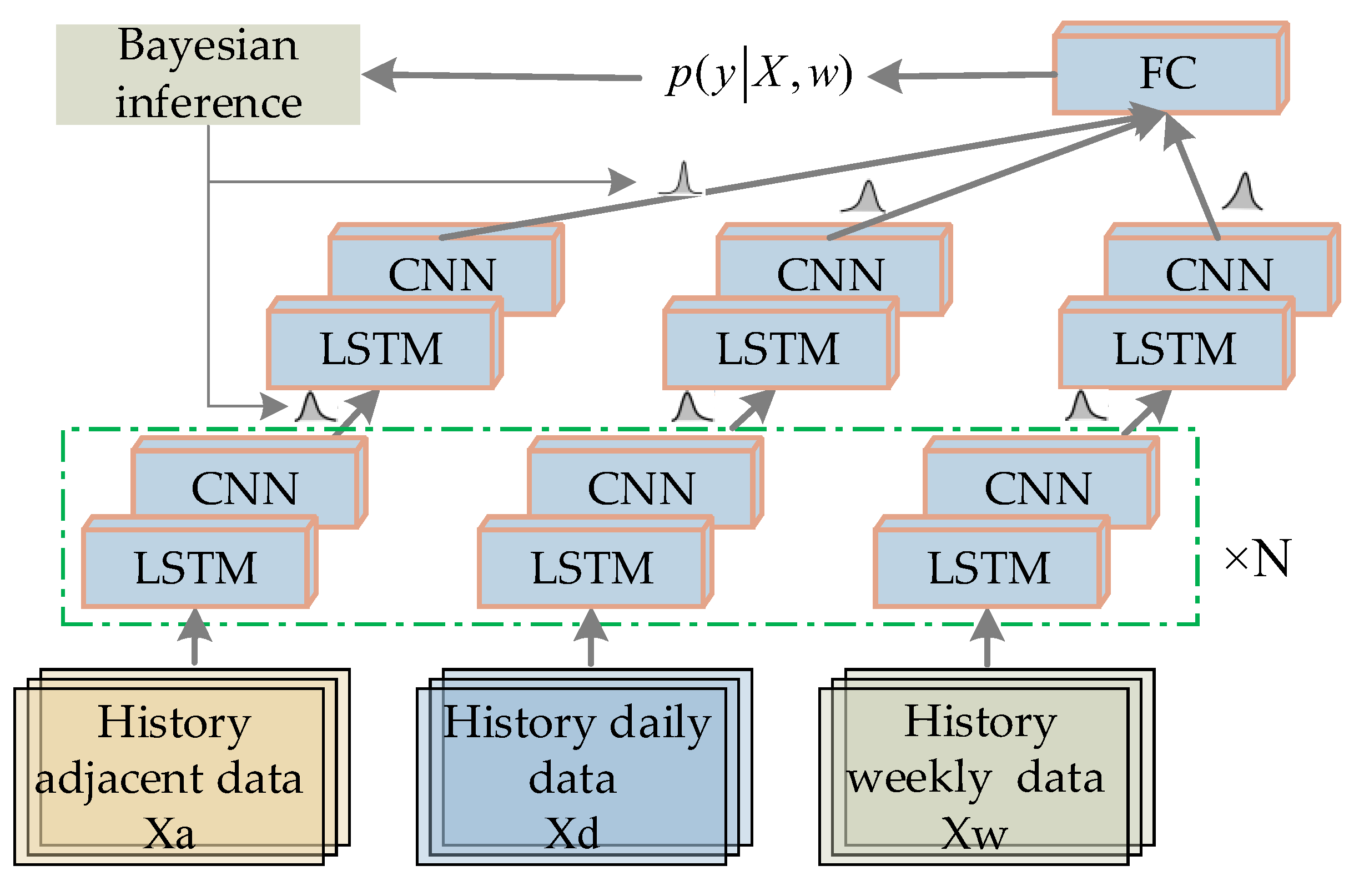
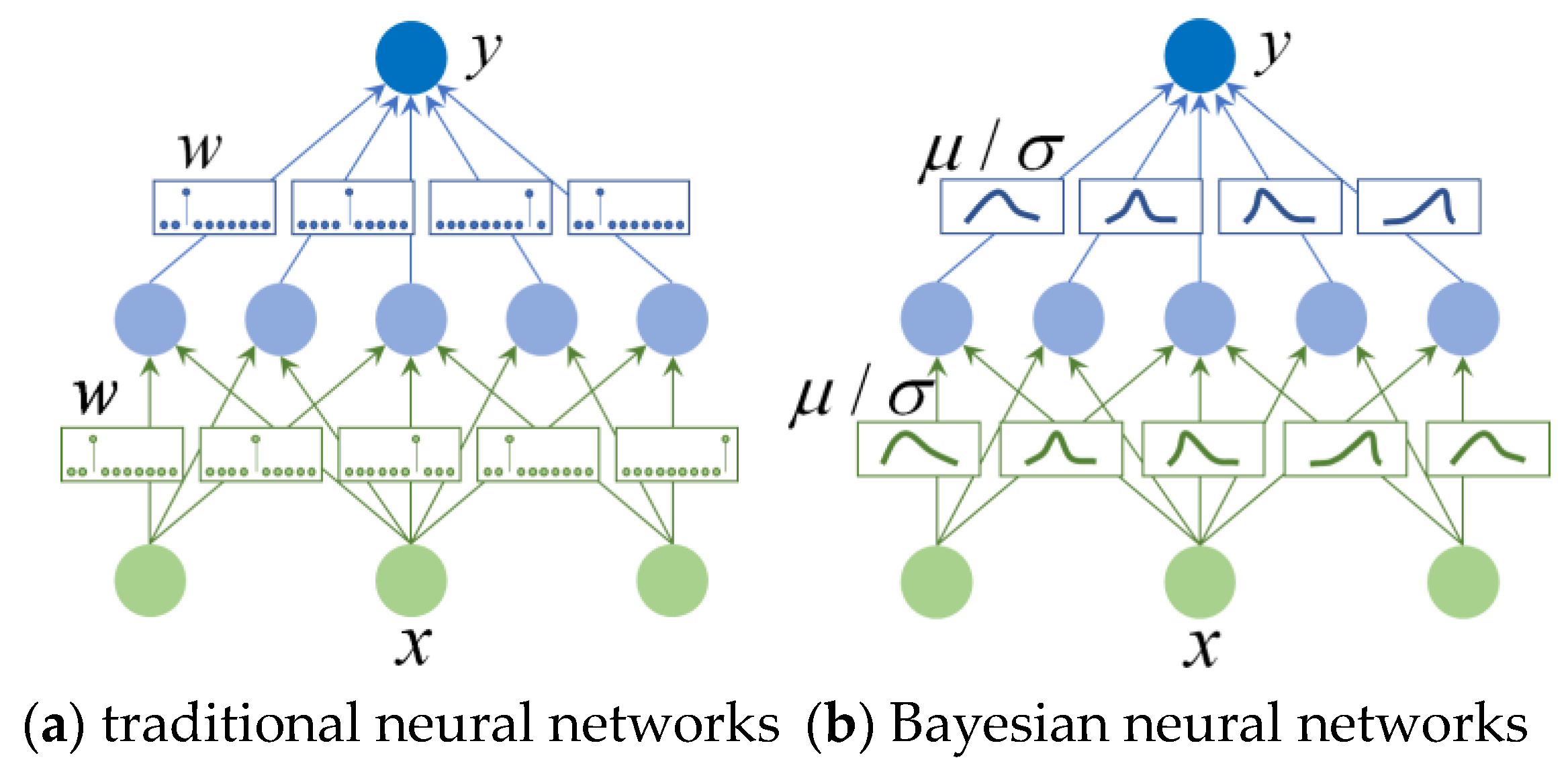
2.3. Bayesian LSTM-CNN

The Bayesian LSTM-CNN prediction model serves as the core component of our proposed methodology for predicting urban interrupted traffic flow. This model is designed to capture the stochasticity and variation present in the traffic flow data, enabling more accurate and reliable predictions.

The architecture of the Bayesian LSTM-CNN model combines two powerful deep learning techniques: Long Short-Term Memory (LSTM) [17] and the Convolutional Neural Network (CNN) [18]. This model uses LSTM to extract the temporal change characteristics of traffic flow and the CNN to extract the spatial change characteristics of traffic flow, and we extend the existing LSTM-CNN architecture to a probabilistic model that better captures the inherent stochasticity and variation in the data. The framework prediction model is shown in Figure 3. The model divides the traffic flow data into three modules and extracts the proximity characteristics, daily periodicity, and periodicity of the traffic flow, respectively.

LSTM is a type of Recurrent Neural Network (RNN), a model frequently employed for processing time series data due to its ability to manage data with temporal relationships. RNNs, however, are limited to short-term memory due to the issue of gradient vanishing. LSTM networks ingeniously address this issue by integrating short-term and long-term memory through a gating mechanism, enabling the learning of long-term dependencies. The primary mechanism of LSTM is this gating system, which incorporates three gates: the input gate, the forget gate, and the output gate. In the context of traffic flow prediction using LSTM, the input gate captures current traffic flow information, while the forget gate retains historical traffic flow data from the time series. This approach enhances the model’s capacity to process time series data.

A three-dimensional spatiotemporal matrix, denoted as $X\in R^{Q\times N\times F_{channel}}$, and $Y\in R^{R\times N}$, is constructed to represent the collected traffic flow data. To capture the temporal dependencies inherent in the traffic flow, a two-layer LSTM network is employed. The network is designed to extract relevant temporal patterns and relationships, as follows:

$$Y_{LSTM}=Linear(LSTM(X,input\_size,hidden\_size,num\_layers))$$

(3)

Convolutional Neural Networks (CNNs) have proven to be effective in extracting correlations among pixels in images. This has led many researchers to incorporate CNNs into traffic flow prediction studies. Typically, these CNN-based traffic flow prediction methods require the construction of historical traffic flow data in a grid structure. The CNN is then utilized to uncover the spatiotemporal relationships among these grids. When constructing a traffic flow prediction model that considers the correlation between intersections, not only are the temporal correlation of the traffic flow data in adjacent time series, the daily periodicity, and the weekly periodicity taken into account, but the correlation between upstream and downstream intersections is also considered. An adjacency matrix table that incorporates the true geographical relationship between traffic flows and a correlation table that captures the temporal correlation of traffic flow time series are constructed. These two spatial relationships are combined to form a spatial correlation table that takes into account the upstream and downstream correlations.

To prevent the loss of higher-order features, a residual network is used to connect $Y_{LSTM}$ and $Y_{CNN}$, as follows:

$$Y_{CNN}=BConv(Y_{LSTM},in\_channels,out\_channels,kernel\_size)$$

(4)

$$Y_{out}=Y_{LSTM}+ResNet(Y_{CNN})$$

(5)

In the equation, $Y_{LSTM}\in R^{R\times N\times F_{hidden\_size}}$, $Y_{CNN}\in R^{R\times N\times F_{out\_channels}}$, $Y_{out}\in R^{R\times N}$, $input\_size$ represents the size of input features, $hidden\_size$ denotes the size of the hidden layer in the LSTM network, $num\_layers$ indicates the number of hidden layers in the LSTM network, $in\_channels$ represents the number of channels in the input of the CNN, $out\_channels$ is the number of output channels in the CNN, and $kernel\_size$ represents the kernel size of the CNN, typically chosen as 3 or 5. The LSTM_CNN model’s output combines the spatiotemporal characteristics of the traffic flow while introducing uncertainty to the deep learning model. Additionally, multiple LSTM_CNN modules can be stacked to improve the accuracy of traffic flow prediction.

Bayesian Extension

We propose to extend the LSTM-CNN into a probabilistic model following Bayesian framework by treating the parameters of LSTM-CNN as random variables. Such extension allows the model to better capture the randomness and variation in dynamic data.

In traditional neural networks, the model parameter w is fixed (Figure 4a), meaning there exists an optimal parameter w* that optimizes the model’s performance. During model training, an initial value w₀ is assigned to the model parameters, and the model is trained based on the observed dataset D, causing w to continuously converge towards w*. This process involves learning the optimal model parameters using methods such as maximum likelihood estimation and gradient descent. In contrast, Bayesian neural networks treat each parameter as a Gaussian distribution with a mean of μ and a variance of σ (Figure 4b). While traditional backpropagation neural networks optimize the parameter w, Bayesian neural networks optimize the mean and variance of each parameter. During inference, Bayesian neural networks sample values from each Gaussian distribution to obtain the values of each parameter. At this stage, the Bayesian neural network functions similarly to a traditional backpropagation network. Multiple samples can be taken, allowing for multiple prediction outcomes. These multiple predictions are then averaged to obtain the final prediction result. Figure 4 shows the model architecture of traditional neural networks and Bayesian neural networks. Each parameter is a signal value in traditional neural networks, while each parameter is a probability distribution in Bayesian neutral networks. Thus, Bayesian neural networks can be considered a special case of ensemble learning. The main motivation behind ensemble learning comes from the observation that aggregating the predictions of a large set of average-performing but independent predictors can lead to better predictions than a single well-performing expert predictor [19].

Suppose X and Y are random variables representing the observed history traffic flow sequence and the corresponding prediction sequence, respectively. Bayesian LSTM-CNN model defines a conditional likelihood $P(Y\left|X,w\right.)$, which specifies the probability of Y given X. w includes all the parameters of LSTM and CNN. w is treated as a random variable following the standard Gaussian as prior, i.e., $P(w)~\mathrm{N}(\mu ,{\sigma }^2)$. Prediction using Bayesian LSTM-CNN can be formulated as a Bayesian inference problem. Given a set of training data $D=\left\{X_i,Y_i\right\}$ and a query of prediction data Y*, the objective of Bayesian inference is to compute the conditional posterior distribution of target variable Y* as follows [20].

$$\mathrm{P}(Y^{*}|X^{*},\mathrm{D})={\displaystyle {\int }_w\mathrm{P}(Y^{*}|X^{*},\mathrm{w}\left)\mathrm{P}\right(\mathrm{w}|D)\mathrm{dw}}$$

(6)

$$P(w|D)=\frac{\mathrm{P}(w)+\mathrm{P}(D\left|w\right)}{P(D)}$$

(7)

Equation (6) uses Monte Carlo estimation to approximate the integration over w. Then the predicted value is as follows.

$$Y^{*}=\frac{1}{M}avg({\displaystyle \sum _{m=1}^M\mathrm{P}(Y^{*}\left|X^{*}{,\mathrm{w}}_m\right)})$$

(8)

where M is the total number of samples of parameters.

The key to perform Bayesian inference is generating samples of parameters w from the posterior distribution. In this work, we use stochastic gradient Hamiltonian Monte Carlo (SGHMC) [21] to approximate inference the posterior distribution.

3. Results

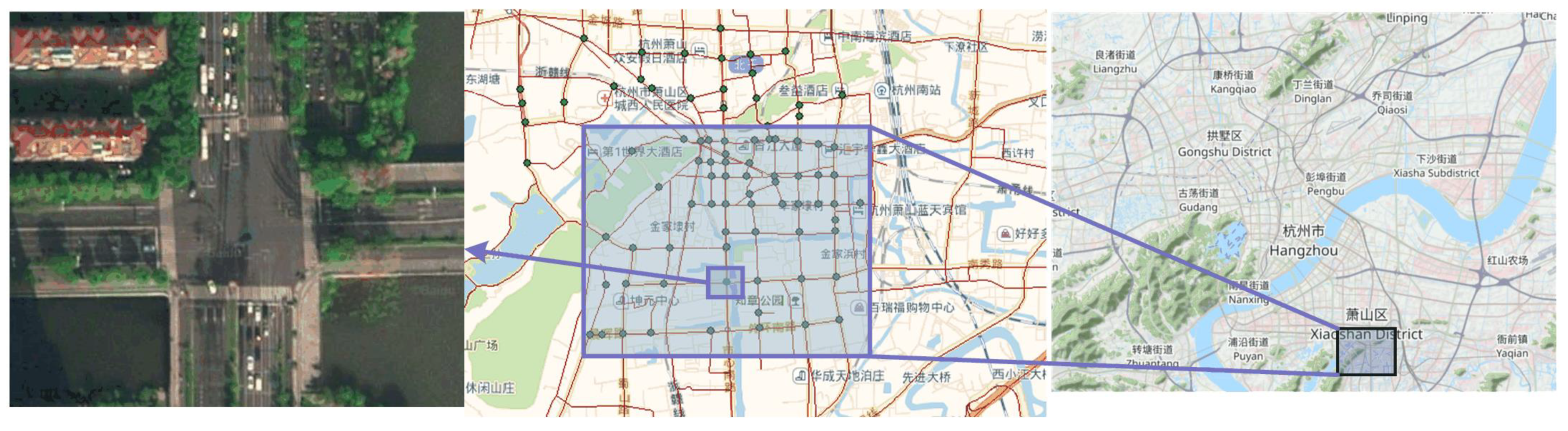
3.1. Data Collection

The dataset used in this study is the license plate recognition (LPR) dataset from Xiaoshan District, Hangzhou, China. The data was collected from 1 April to 31 July 2019, spanning a total of four months.

To investigate short-term traffic flow prediction on the signal intersection, the intersection of Shixin Road with Nanxiu Road and an area with 266 intersections were selected as the target intersection and the area for the study, respectively. The location of the study area is depicted in Figure 5.

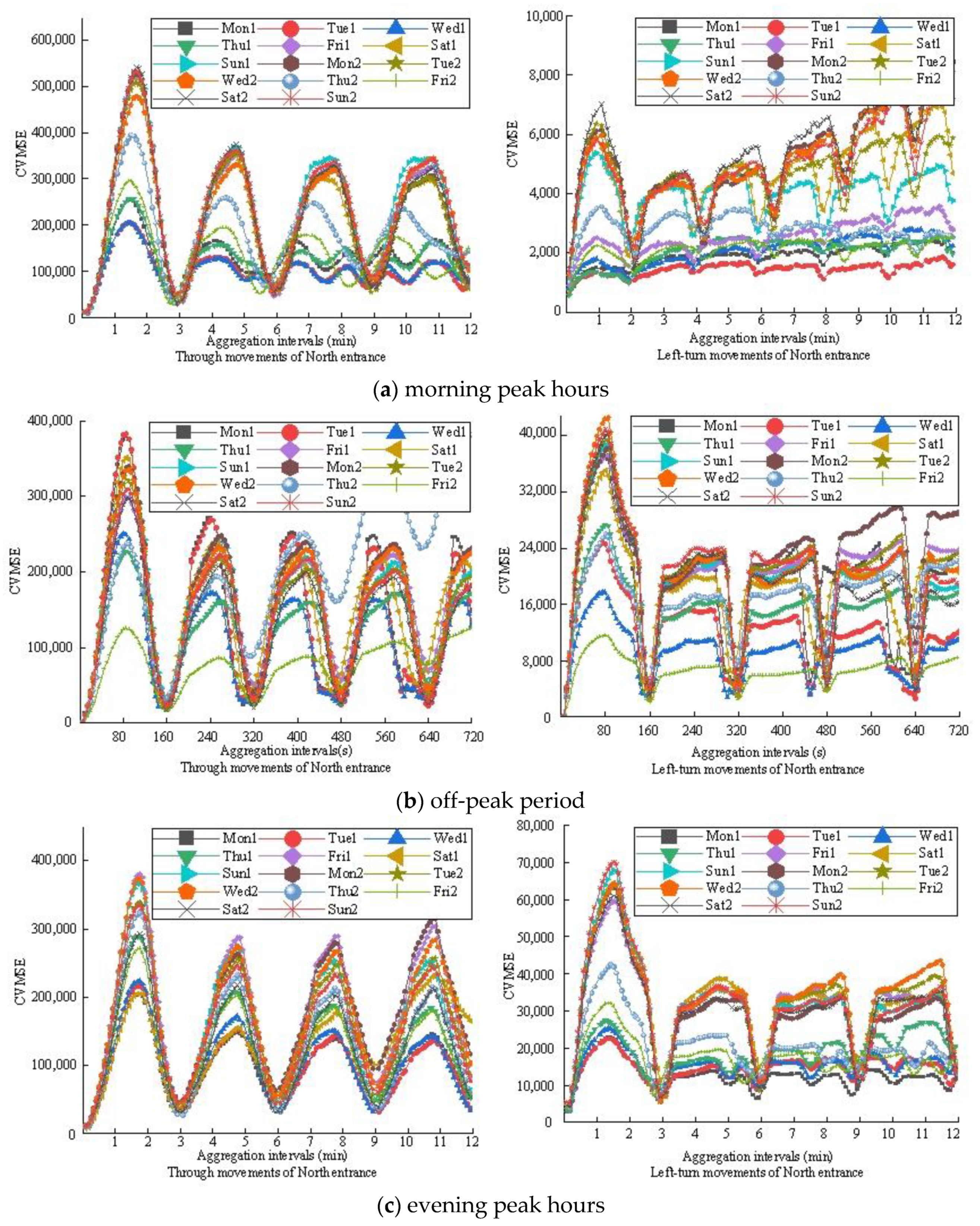
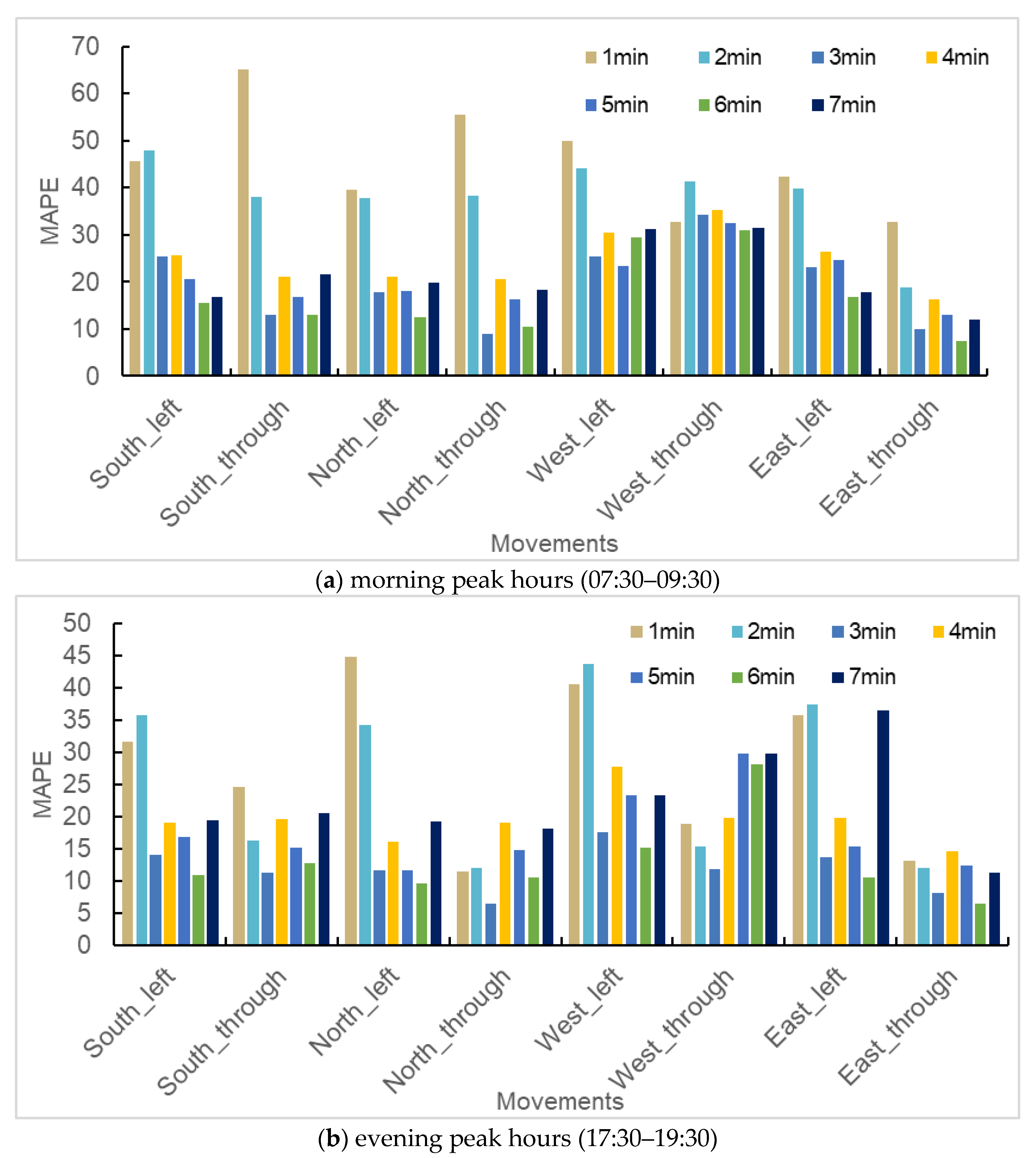
3.2. Optimal Aggregation Time Interval

3.2.1. Single Intersection Scenario

The traffic flow data from the intersection, spanning from 1 April 2019 to 7 April 2019, during both peak (07:30–09:30, 17:30–19:30) and off-peak hours (10:00–12:00), serve as the basis for our analysis. The original license plate recognition data were collected based on the traffic flow every 5 s as the minimum collection time window. We calculated the CVMSE for different turning traffic flows. Figure 6a shows the CVMSE for different turning traffic flows at the intersection during the morning peak, Figure 6b during the off-peak period, and Figure 6c during the evening peak. As per Figure 6a, during the morning peak period, the minimum CVMSE at the intersection was observed when the aggregation time intervals are 3 min, 6 min, 9 min, and 12 min. Consequently, these intervals were deemed the optimal aggregation time intervals for this target intersection during the morning peak.

In a similar vein, Figure 6b indicates that, during the off-peak period, the minimum CVMSE at the intersection was achieved when the aggregation time intervals were 160 s, 320 s, 480 s, and 640 s. Therefore, these intervals were identified as the optimal aggregation time intervals for this intersection during the off-peak period. Correspondingly, Figure 6c reveals that, during the evening peak period, the minimum CVMSE at the target intersection was observed when the aggregation time intervals are 3 min, 6 min, 9 min, and 12 min. As such, these intervals were determined to be the optimal aggregation time intervals for this target intersection during the evening peak.

The signal control cycle at the intersection during the morning and evening peak hours was 180 s, and during the off-peak period from 10:00–12:00, it was 160 s. Consequently, the optimal collection time interval at the signal-controlled intersection is a multiple of the signal control cycle.

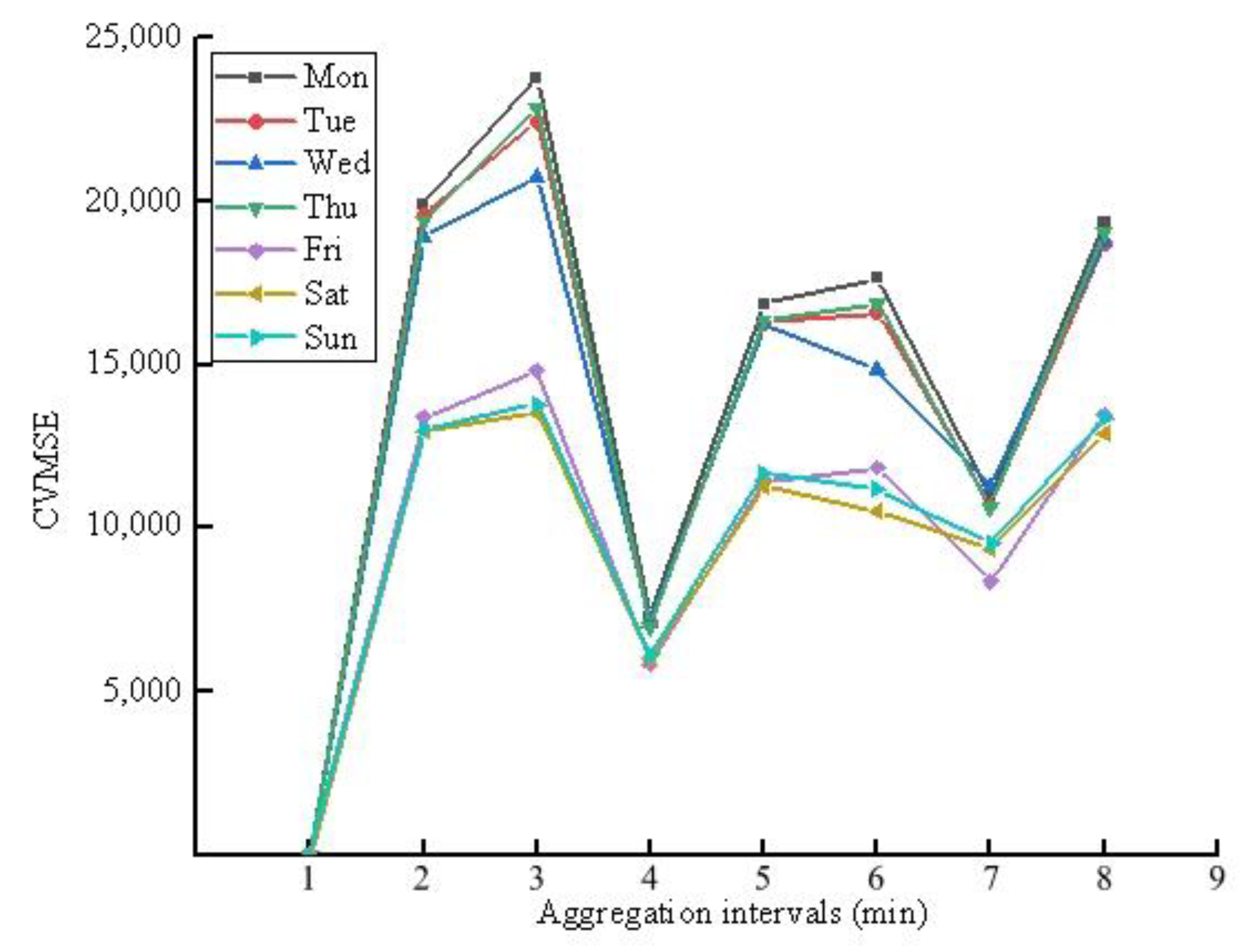
3.2.2. Network Scenario

The study examined the optimal aggregation time interval for short-term traffic flow in the road network. To achieve this, the original license plate recognition dataset was aggregated into the minimum time window of 1 min. The optimal aggregation time interval for the road network traffic flow was determined using CVMSE analysis. Figure 6 illustrates the CVMSE for the entire 24 h period in the selected area when the aggregation time interval ranged from 1 to 8 min.

According to the analysis in Figure 7, it can be observed that, when considering the entire day as the study period, the traffic flow in the selected area exhibited the lowest CVMSE when the aggregation time interval was set to 4 min. This value is significantly lower compared to the CVMSE at aggregation time intervals of 3 min and 5 min. Interestingly, when the aggregation time interval was set to the commonly used 5 min in traditional prediction models, the CVMSE for the traffic flow increases. Additionally, the CVMSE was relatively small when the aggregation time interval was set to 7 min. Therefore, based on these findings, the optimal aggregation time interval for short-term traffic flow in the studied road network area was determined to be 4 min.

3.3. Prediction Results

3.3.1. Evaluation Metrics

We applied three widely used metrics to evaluate the performance of our model, including the mean absolute error (MAE), root mean square error (RMSE), and mean absolute percentage error (MAPE). The formulas are as follows:

$$\mathrm{MAE}=\frac{1}{n}{\displaystyle \sum _{i=0}^n|y_i-\overline{y_i}}|,$$

(9)

$$\mathrm{RMSE}=\frac{1}{n}{\displaystyle \sum _{i=0}^n\sqrt{{(y_i-y_i)}^2}},$$

(10)

$$\mathrm{MAPE}=\frac{1}{n}{\displaystyle \sum _{i=0}^n|\frac{y_i-\overline{y_i}}{y_i}}|.$$

(11)

3.3.2. Benchmark Methods

To validate the generalization ability of the Bayesian LSTM_CNN model, this study selected the following benchmark models for comparison:

ARIMA [22]: Autoregressive Integrated Moving Average (ARIMA) is a time series forecasting model that incorporates differencing, autoregression, and moving average components.

SVR [23]: Support Vector Regression (SVR) is another classical time series analysis model that uses linear support vector machines for regression tasks.

KNN [24]: The K-Nearest Neighbors (KNN) algorithm is a machine learning algorithm that can be used for both classification and regression. It finds the K nearest training samples based on distance metrics and makes predictions based on information from these “neighbors”.

LSTM [6]: Long Short-Term Memory (LSTM) is a special type of recurrent neural network (RNN) that effectively addresses the long-term dependency problem and is commonly used in time series forecasting.

ASTGCN [25]: An Attention-based Spatial-Temporal Graph Convolutional Network (ASTGCN) is a deep learning model proposed in 2019 that combines graph convolutional networks, convolutional neural networks, and attention mechanisms.

Graph-Wavenet [26]: Graph-WaveNet is a novel graph neural network architecture for modeling spatiotemporal graphs. It introduces an adaptive dependency matrix to capture hidden spatial dependencies in the data.

STSGCN [27]: A Spatial-Temporal Synchronous Graph Convolutional Network (STSGCN) is a deep learning model that addresses the heterogeneity of spatiotemporal networks in the time dimension. It utilizes graph signal matrices to capture spatiotemporal features and constructs multi-module layers to capture long-range spatiotemporal network heterogeneity.

DGCRN [28]: A Dynamic Graph Convolutional Recurrent Network (DGCRN) is a new traffic forecasting framework that combines dynamic graph convolutional recurrent networks. In DGCRN, a hypernetwork is designed to utilize and extract dynamic features of node attributes, and the parameters of dynamic filters are generated at each time step. It filters the node embeddings to generate dynamic graphs and integrates them with predefined static graphs.

3.3.3. Parameter Settings

In this paper, single-step prediction is used to predict the traffic flow data of the next time series by using the traffic flow data of the historical time series, where Xa = 12, Xd = 1, Xw = 1, which means that the traffic flow data of the first 12 time series adjacent to the predicted time point, the traffic flow data of the same time point of the previous day, and the traffic flow data of the same time point of the previous week are taken into account during the prediction. In the Bayesian LSTM-CNN model, the dimension of the hidden layer state in the LSTM network is 16, and the number of layers of LSTM is set to 8. The dimension of the hidden layer state in the CNN is set to 16, the filling size is set to 2, and the convolution core size is 3. The initial value of each parameter follows the standard normal distribution N (0, 1) with a mean value of 0 and a variance of 1. The initial learning rate is 0.001. We decay the rate by 0.9 every 100 epochs. The batch size is set as 64. Dropout is applied to the input and output of LSTM to further prevent overfitting, and the dropout rate is set as 0.2. All the hyper-parameters of the proposed neural network are optimized by grid search, which is a traditional method that performs hyperparameter tuning to determine the optimal values for a given model.

3.3.4. Results

Performance on Signal Intersection

We conducted an analysis of the Bayesian LSTM-CNN model predictive accuracy for different turning traffic flows at intersections, considering various aggregation time intervals, with the findings depicted in Figure 8. It was commonly observed that traffic flow was more volatile at smaller aggregation time intervals and stabilized as the interval increases. Nonetheless, Figure 8 indicates that the Mean Absolute Percentage Error (MAPE) was notably lower at an aggregation time interval of 3 min compared to 2 or 4 min. In a similar pattern, a 6 min interval resulted in a lower MAPE than intervals of 5 or 7 min. Given that the signal control cycle during peak morning and evening hours at the intersection was 3 min, the traffic flow predictions were most accurate when the aggregation time interval aligned as a multiple of the signal control period.

Table 1. Comparison of MAE predicted by different prediction models at intersection.

Model	ARIMA	SVR	KNN	CapsNet	GRU	STAWnet	Ours
South_left	3.99	3.32	3.41	3.52	3.15	3.11	3.07
South_through	11.54	7.62	8.16	10.03	7.31	8.12	7.20
North_left	3.61	3.09	3.25	3.17	2.99	3.09	3.03
North_through	13.75	9.29	9.59	12.53	8.78	9.55	8.75
West_left	4.27	3.36	3.33	4.19	3.24	3.17	3.20
West_through	1.93	1.86	1.82	1.87	1.62	1.74	1.66
East_left	2.29	2.17	2.34	2.19	2.15	2.19	2.04
East_through	3.91	3.65	3.84	3.74	3.51	3.70	3.45
Mean	5.66	4.29	4.47	5.15	4.19	4.32	4.09

and

Table 2. Comparison of RMSE predicted by different prediction models at intersection.

Model	ARIMA	SVR	KNN	CapsNet	GRU	STAWnet	Ours
South_left	4.98	4.25	4.33	4.27	4.05	3.86	3.72
South_through	14.40	9.86	10.38	12.35	9.55	10.28	9.26
North_left	4.54	3.81	4.00	3.84	3.69	3.63	3.47
North_through	16.83	11.92	12.16	15.12	11.34	12.35	11.09
West_left	5.46	4.24	4.24	5.32	3.99	3.97	3.78
West_through	2.43	2.18	2.14	2.30	2.05	2.02	1.84
East_left	2.86	2.71	2.81	2.78	2.64	2.68	2.38
East_through	4.83	4.47	4.62	4.59	4.25	4.52	4.07
Mean	7.04	5.43	5.58	6.32	5.20	5.41	4.95

show the MAE, RMSE, and MAPE values of different prediction models at the intersection when the traffic flow aggregation interval is 3 min. According to the tables, compared with other state-of-the-art prediction models, the Bayesian LSTM-CNN model has the best prediction accuracy.

Performance on Network Performance

According to the results of Section 3.2.2, the CVMSE of the traffic flow data in this area was smallest when the aggregation time interval was 4 min, and it was relatively small when the aggregation time interval was 7 min. Therefore, to analyze the impact of different aggregation time intervals on the prediction results of the regional road network, the traffic flow was aggregated into data with time intervals of 3–7 min, and the Bayesian LSTM_CNN model proposed in this paper was used to predict the short-term traffic flow of traffic flow data with different aggregation time intervals. The prediction results are shown in

Table 3. Bayesian LSTM-CNN model prediction metrics of the study area traffic flow at different aggregation intervals.

Aggregation Intervals	Metrics
	MAE	RMSE	MAPE
3 min	3.83	4.38	28.87
4 min	3.50	4.26	25.65
5 min	3.67	5.30	26.59
6 min	4.77	5.95	26.42
7 min	4.09	6.50	25.25
8 min	4.82	7.20	27.98

.

Comparative analysis of the prediction results of the benchmark model: The prediction results of the road network traffic flow data for the whole day were analyzed.

Table 4. Prediction results of short-term traffic flow benchmark model in an urban road network.

Interval	Metrics	ARIMA	KNN	SVR	LSTM	ASTGCN	STSGCN	Graph-Wavenet	DGCRN	Ours
4 min	MAE	4.29	5.23	4.89	4.26	4.12	4.42	4.21	4.13	3.50
	RMSE	6.26	7.13	6.69	6.12	5.94	6.36	5.96	5.79	4.26
	MAPE	30.35	37.71	35.83	28.48	26.43	28.49	26.15	26.29	25.65
7 min	MAE	4.25	5.19	4.85	4.20	4.07	4.39	4.08	4.04	3.17
	RMSE	6.01	7.02	6.56	6.05	5.94	6.31	5.88	5.48	4.18
	MAPE	30.26	37.59	35.73	28.35	26.31	28.35	26.09	26.18	25.60

is the prediction result of this area when the aggregation time interval was 4 min and 7 min. As can be seen from the table, compared with some benchmark prediction models, the MAE, RMSE, and MAPE of the Bayesian LSTM_CNN model is relatively low. The Bayesian LSTM_CNN model presents better prediction results for short-term traffic flow prediction on the road network.

4. Conclusions

This paper introduces a method for predicting urban interrupted traffic flow, which is based on Bayesian deep learning and considers the optimal aggregation time interval. Specifically, this method utilizes the cross-validation mean square error (CVMSE) method to obtain the optimal aggregation time interval. A Bayesian LSTM-CNN prediction model, which extends the LSTM-CNN model under the Bayesian framework to a probabilistic model to better capture the stochasticity and variation in the data, is proposed. The model is verified based on license plate recognition data. The results show that the optimal aggregation time interval of traffic flow at urban signalized intersections is a multiple of the signal control cycle. The collection and processing of urban interrupted traffic flow data based on the optimal aggregation time interval can effectively improve the prediction accuracy of different prediction models. The proposed prediction model that combines Bayesian inference and deep learning model proposed in this paper takes into account the space-time correlation and uncertainty of traffic flow, and the prediction results are better than the state-of-the-art models, which improves the prediction accuracy. The prediction results can provide a reference for the optimization of signal control schemes and have good practicability. However, this paper has some limitations. The signal control scheme of the study case in this paper is a multi-period control scheme, and the relevant research on the dynamic and real-time signal control scheme needs further testing and verification in the future.

References

1. Stathopoulos, A.; Karlaftis, M.G. A multivariate state space approach for urban traffic flow modeling and prediction. Transp. Res. Part C Emerg. Technol. 2003, 11, 121–135. [Google Scholar] [CrossRef]
2. Chen, M.; Chien, S. Dynamic Freeway Travel-Time Prediction with Probe Vehicle Data: Link Based Versus Path Based. Transp. Res. Rec. J. Transp. Res. Board 2001, 1768, 157–161. [Google Scholar] [CrossRef]
3. Kamarianakis, Y.; Prastacos, P. Forecasting traffic flow conditions in an urban network: Comparison of multivariate and univariate approaches. Transp. Res. Rec. J. Transp. Res. Board 2003, 1857, 74–84. [Google Scholar] [CrossRef]
4. Asif, M.T.; Dauwels, J.; Goh, C.Y.; Oran, A.; Fathi, E.; Xu, M.; Dhanya, M.M.; Mitrovic, N.; Jaillet, P. Spatiotemporal patterns in large-scale traffic speed prediction. IEEE Trans. Intell. Transp. Syst. 2014, 15, 794–804. [Google Scholar] [CrossRef]
5. Zheng, Z.; Su, D. Short-term traffic volume forecasting: A k-nearest neighbor approach enhanced by constrained linearly sewing principle component algorithm. Transp. Res. Part C Emerg. Technol. 2014, 43, 143–157. [Google Scholar] [CrossRef]
6. Zhao, Z.; Chen, W.; Wu, X.; Chen, P.C.Y.; Liu, J. LSTM network:a deep learning approach for short-term traffic forecast. IET Intell. Transp. Syst. 2017, 11, 68–75. [Google Scholar] [CrossRef]
7. Tian, C.; Chan, W. Spatial-temporal attention wavenet: A deep learning framework for traffic prediction considering spatial-temporal dependencies. IET Intell. Transp. Syst. 2021, 15, 549–561. [Google Scholar] [CrossRef]
8. Tang, J.; Zeng, J. Spatiotemporal gated graph attention. network for urban traffic flow prediction based on license plate recognition data. Comput. Aided Civ. Infrastruct. Eng. 2022, 37, 3–23. [Google Scholar] [CrossRef]
9. Zellner, A.; Montmarquette, C. A study of some aspects of temporal aggregation problems in econometric analyses. Rev. Econ. Stat. 1971, 53, 335–342. [Google Scholar] [CrossRef]
10. Rossana, R.J.; Seater, J.J. Temporal aggregation and economic time series. J. Bus. Econ. Stat. 1995, 13, 441–451. [Google Scholar]
11. Vlahogianni, E.I.; Karlaftis, M.G.; Golias, J.C. Statistical methods for detecting nonlinearity and nonstationarity in univariate short-term time-series of traffic volume. Transp. Res. Part C 2006, 14, 351–367. [Google Scholar] [CrossRef]
12. Byron, J.; Shawn, M.; William, L.; Clifford, S. Intelligent Transportation System data archiving: Statistical techniques for determining optimalaggregation widths for inductance loop detectors. Transp. Res. Rec. 2000, 1719, 85–93. [Google Scholar]
13. Park, D.; Rilett, L.; Gajewski, B.; Spiegelman, C.; Choi, C. Identifying optimal data aggregation interval sizes for link and corridor travel time estimation and forecasting. Transportation 2009, 36, 77–95. [Google Scholar] [CrossRef]
14. Smith, B.; Ulmer, J. Freeway traffic flow rate measurement: Investigation into impact of measurement time interval. J. Transp. Eng. 2003, 129, 223–229. [Google Scholar] [CrossRef]
15. Yu, L.; Chen, X.-M.; Grng, Y.-B. Data integration method of intelligent transportation system based on wavelet decomposition. J. Tsinghua Univ. Nat. Sci. Ed. 2004, 44, 793–796. [Google Scholar]
16. Weerasekera, R.; Sridharan, M.; Ranjitkar, P. Implications of spatiotemporal data aggregation on short-term traffic prediction using machine learning algorithms. J. Adv. Transp. 2020, 2020, 1–21. [Google Scholar] [CrossRef]
17. Hochreiter, S.; Schmidhuber, J. Long short-term memory. Neural Comput. 1997, 9, 1735–1780. [Google Scholar] [CrossRef] [PubMed]
18. Kim, Y. Convolutional neural networks for sentence classification. arXiv 2014, arXiv:1408.5882. [Google Scholar]
19. Jospin, L.V.; Laga, H.; Boussaid, F.; Buntine, W.; Bennamoun, M. Hands-on Bayesian neural networks—A tutorial for deep learning users. IEEE Comput. Intell. Mag. 2022, 17, 29–48. [Google Scholar] [CrossRef]
20. Gelman, A.; Stern, H.S.; Carlin, J.B.; Dunson, D.B.; Vehtari, A.; Rubin, D.B. Bayesian Data Analysis; Chapman and Hall/CRC: New York, NY, USA, 2013. [Google Scholar]
21. Chen, T.; Fox, E.; Guestrin, C. Stochastic gradient hamiltonian monte carlo. Proc. Mach. Learn. Res. 2014, 32, 1683–1691. [Google Scholar]
22. Kumar, S.V.; Vanajakshi, L. Short-term traffic flow prediction using seasonal ARIMA model with limited input data. Eur. Transp. Res. Rev. 2015, 7, 1–9. [Google Scholar] [CrossRef]
23. Toan, T.D.; Truong, V.H. Support vector machine for short-term traffic flow prediction and improvement of its model training using nearest neighbor approach. Transp. Res. Rec. 2021, 2675, 362–373. [Google Scholar] [CrossRef]
24. Cheng, S.F.; Lu, F.; Peng, P.; Wu, S. Short-term traffic forecasting: An adaptive ST-KNN model that considers spatial heterogeneity. Comput. Environ. Urban Syst. 2018, 71, 186–198. [Google Scholar] [CrossRef]
25. Guo, S.N.; Lin, Y.F.; Li, S.J.; Chen, Z.; Wan, H. Deep Spatial-Temporal 3D Convolutional Neural Networks for Traffic Data Forecasting. IEEE Trans. Intell. Transp. Syst. 2021, 20, 3913–3926. [Google Scholar] [CrossRef]
26. Wu, Z.H.; Pan, S.R.; Long, G.D.; Jiang, J.; Zhang, C. Graph WaveNet for Deep Spatial-Temporal Graph Modeling. arXiv 2019, arXiv:1906.00121. [Google Scholar]
27. Song, C.; Lin, Y.; Guo, S.; Wan, H. Spatial-temporal synchronous graph convolutional networks: A new framework for spatial-temporal network data forecasting. Proc. AAAI Conf. Artif. Intell. 2020, 34, 914–921. [Google Scholar] [CrossRef]
28. Li, F.; Feng, J.; Yan, H.; Jin, G.; Yang, F.; Sun, F.; Jin, D.; Li, Y. Dynamic Graph Convolutional Recurrent Network for Traffic Prediction: Benchmark and Solution. IEEE Trans. Knowl. Eng. 2021, 17, 1–21. [Google Scholar] [CrossRef]
Figure 1. Overall framework of the proposed model.
Sustainability 16 01818 g001
Figure 2. Example of CVMSE calculation process with 1 min.
Sustainability 16 01818 g002
Figure 3. Bayesian LSTM-CNN forecasting model architecture. FC means “Fully Connected”. The curve symbol means distribution.
Sustainability 16 01818 g003
Figure 4. Model architecture of traditional neural networks and Bayesian neural networks. The circles in the box means a definite value, and the curve in the box means distribution.
Sustainability 16 01818 g004
Figure 5. The location of the study area in Hangzhou city. The Non-english terms in the figure are the place names in Chinese.
Sustainability 16 01818 g005
Figure 6. CVMSE of the intersection traffic flow at different aggregation intervals in different periods.
Sustainability 16 01818 g006
Figure 7. CVMSE of the study area traffic flow at different aggregation intervals.
Sustainability 16 01818 g007
Figure 8. MAPE of Bayesian LSTM-CNN model prediction of the study intersection traffic flow at different aggregation intervals.
Sustainability 16 01818 g008