The Temporal–Spatial Evolution Characteristics and Influential Factors of Carbon Imbalance in China

Abstract

The ongoing progress of industrialization and urbanization has exacerbated the imbalance between carbon emissions and absorption, leading to heightened risks of climate change, such as frequent occurrences of extreme weather events. Clarifying the driving forces and temporal–spatial evolution characteristics of China’s carbon balance holds significant theoretical value in understanding the systemic nature and patterns of interaction between carbon emissions and absorption. We utilize provincial panel data from 2005 to 2021 in China and a spatial Durbin model to explore the spatial spillover effects of carbon imbalance and its influencing factors. The results indicate a gradual exacerbation of carbon imbalance in China over time. There exists a spatially positive correlation pattern in provincial carbon imbalance distribution. From 2005 to 2010, intra-regional differences in carbon imbalance levels were a significant contributor to China’s overall carbon imbalance disparity, while from 2011 to 2019, inter-regional differences played a more substantial role. Given the apparent phenomena of population aggregation, industrial concentration, and economic interdependence among provinces, changes in population size, economic growth, and industrial structure exacerbate the level of carbon imbalance in spatially correlated regions. Conversely, due to knowledge and technology spillovers, improvements in energy efficiency facilitated by the flow of production factors like capital aid in the governance of carbon imbalance in spatially associated areas. We emphasize that local governments should focus on a regional integration perspective in carbon imbalance governance and strategically coordinate with neighboring provinces and cities to advance carbon imbalance governance. The findings provide theoretical support for understanding and effectively managing the situation of carbon imbalance in China.

1. Introduction

Since the industrial revolution, human activities, especially the substantial consumption of fossil fuels by developed nations, have led to a significant accumulation of carbon dioxide emissions in the atmosphere, intensifying global climate change which is primarily characterized by warming trends. Greenhouse gas emissions have resulted in increased occurrences of extreme weather events and frequent natural disasters, contributing to adverse climate changes. The alterations in meteorological elements such as temperature, radiation, precipitation, and wind speed triggered by climate change, in turn, impact the generation and transmission of pollutants, exacerbating regional air pollution levels and posing a threat to human health.

The emission of greenhouse gases, primarily carbon dioxide, has led to global climate warming, posing a severe threat to human existence and sustainable development, standing as one of the significant global challenges humanity faces today. The milestone significance of the 2016 international treaty, the Paris Agreement, signifies the collective global concern for climate change, and the transition towards green and low-carbon development has become a widespread consensus among nations.

In 2020, China accounted for approximately 30% of global carbon emissions. Concurrently, China’s energy consumption per unit of gross domestic product (GDP) stood at 3.4 tons of standard coal per USD ten thousand, with a carbon dioxide emissions intensity of 6.7 tons per USD ten thousand of GDP, which are 1.5 times and 1.8 times higher than the world average, respectively. China has only a 30-year transition period from carbon peaking to carbon neutrality, facing more stringent and extensive emission reduction requirements than developed countries within a tighter timeframe. However, on the one hand, as the spatial scope of end-of-pipe pollution control measures diminishes, the marginal costs of further environmental benefits and the difficulty of emission reduction increase. China faces dual pressures to achieve carbon neutrality goals while ensuring environmental pollution prevention and control. On the other hand, due to cost and technological limitations, large-scale market applications of “end-of-pipe” carbon capture and storage technologies for greenhouse gas emission reduction remain challenging, and carbon sequestration capacity remains insufficient. Therefore, the escalating climate issues in China fundamentally stem from the contradiction between excessive consumption of fossil fuels and inadequate carbon sequestration capacities, resulting in carbon imbalance. Some argue that the disparities in carbon imbalance among different regions became more pronounced between 2011 and 2019, whereas such differences were not as significant before 2010 [1,2]. Consequently, we aim to delve deeper into the temporal–spatial evolution characteristics of China’s carbon imbalance and its driving factors, aiming to provide a scientific basis for addressing climate change, environmental protection, and sustainable development.

The existing literature has extensively delved into the spatiotemporal evolution characteristics of carbon emissions [3,4,5,6] and their intricate impact mechanisms [7,8,9]. The study in [10] examined the potential influences of energy poverty, renewable energy consumption, GDP, natural gas consumption, and trade freedom on carbon emissions, concluding that prioritizing the reduction of energy poverty in developing countries is pivotal for achieving sustainable development goals. The study in [11] employed autoregressive distributed lag models to analyze the influence of political and social factors on carbon emissions, demonstrating that reduced corruption and increased female political participation significantly diminish carbon emissions, while heightened political stability markedly reduces emissions in the short term. Considering China’s status as the largest emitter of carbon, the study in [12] employed production theory decomposition and index decomposition analysis to investigate the underlying driving factors of China’s carbon emissions. Their findings highlight economic activities as the primary contributor to increased emissions, with GDP-related technological changes and energy intensity playing significant roles in most Chinese provinces’ emissions. There are many similar studies [13,14,15,16,17].

However, the continuous progression of industrialization and urbanization has imposed significant pressure for emissions reduction, gradually making the enhancement of carbon sequestration capacity an increasingly scrutinized focal point within academia [18,19,20,21]. The study in [22], drawing upon the theoretical framework of a dynamic stochastic general equilibrium model, discussed the influence of carbon sink insurance and fiscal subsidies on forestry’s carbon sequestration capabilities. Their findings illustrate that carbon sink insurance and premium subsidies can enhance forestry carbon sink capacities, while direct fiscal subsidies and premium subsidies can augment forestry’s carbon sequestration abilities. The study in [23] delved into the spatiotemporal dynamics of the net primary productivity (NPP) and net ecosystem productivity (NEP) of vegetation in the Wei River Basin, quantifying the impact of climate change and human activities on vegetation’s carbon fixation capabilities. The existing literature primarily concentrates on the factors influencing carbon emissions and absorption capacities and their spatiotemporal evolution. However, a systematic examination from a balanced interaction perspective between carbon emissions and absorption, elucidating the mechanisms influencing carbon balance, is lacking. There is a dearth of theoretical mechanism analysis regarding carbon balance, underscoring the significance of unraveling the driving factors and spatiotemporal evolution characteristics of carbon balance in comprehending the systematic nature and patterns of interaction between carbon emissions and absorption.

The main contributions of this work are as follows:

(1)

We innovatively construct a Carbon Imbalance Index at the provincial level in China by utilizing high-spatiotemporal-resolution and dynamically updated global multi-scale databases provided by NASA and the MEIC platform. This approach integrates data on carbon emissions and absorption, offering a new perspective on the carbon imbalance scenario.

(2)

The evolution patterns of carbon emissions and absorption in different regions and periods across China reveal intricate dynamics. By unveiling the dynamic evolution characteristics and spatial disparities in carbon imbalance among Chinese provinces, we aim to comprehend the current status and evolving patterns of carbon imbalance.

(3)

Employing a spatial Durbin model, we identify the driving factors behind China’s carbon imbalance and, from a spatial spillover perspective, elucidate the dynamic interrelationships of carbon imbalance among provincial regions. This analytical approach uncovers the interconnectedness of carbon imbalance dynamics within and between provinces.

2. Materials and Methods

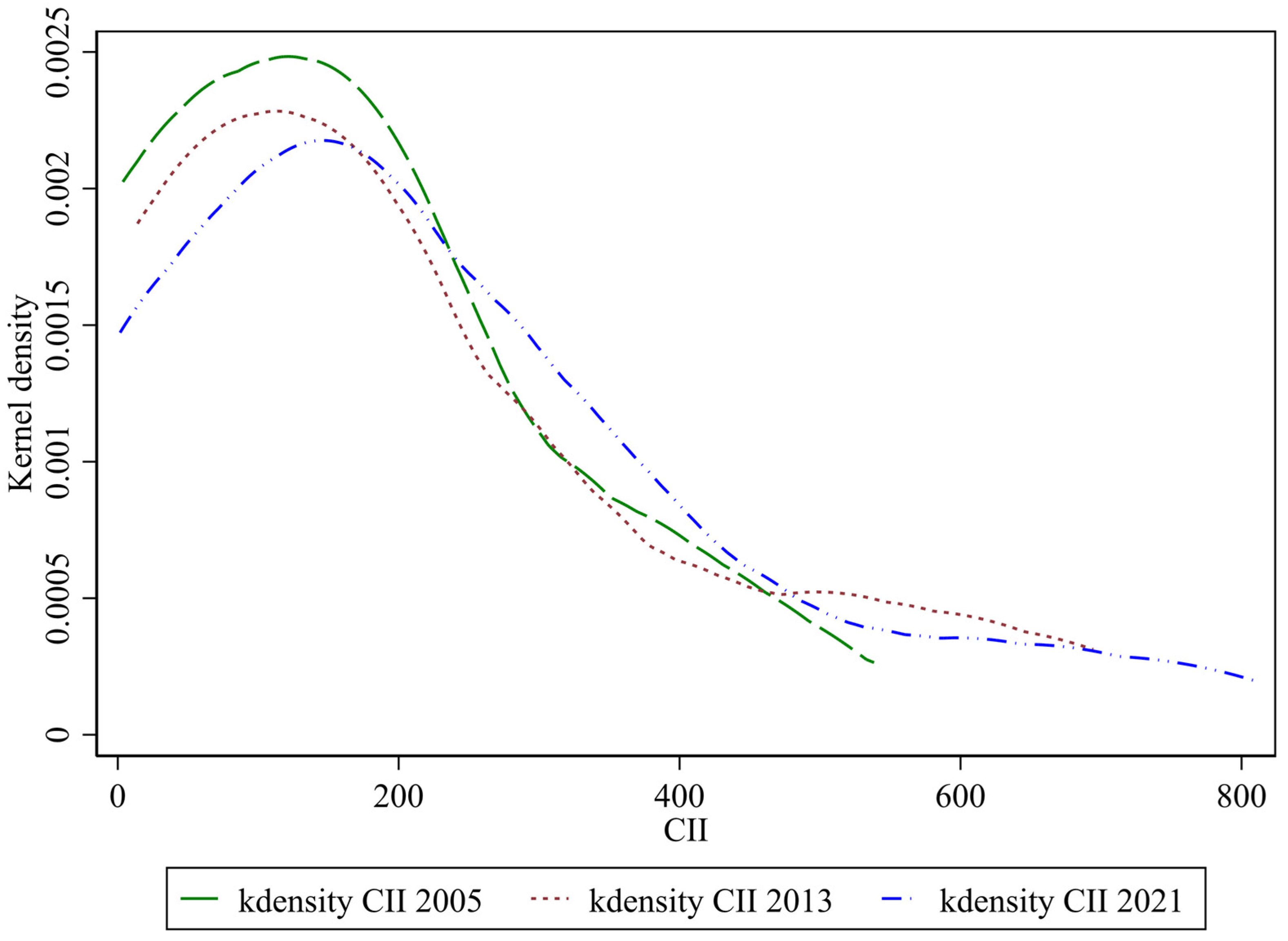
2.1. Kernel Density Estimation

In statistics, Kernel Density Estimation (KDE) is a non-parametric method that applies kernel smoothing to estimate the probability density function of a random variable by using kernels as weights. In this work, the KDE method is employed to analyze the spatiotemporal changes in carbon imbalance in China. Equation (1) is utilized to estimate the kernel density of carbon imbalance.

$$F_g(CII)=\frac{1}{ng}{\displaystyle \sum _{i=1}^{n}K(\frac{CII-CI{I}_i}{g})}$$

(1)

where $K(.)$ represents the Epanechnikov kernel density function, $n$ denotes the number of provinces, $CI{I}_i$ represents the carbon imbalance of the $i$th province, and $g$ is the estimated bandwidth. The study utilizes the optimal bandwidth method to determine the bandwidth.

2.2. Dagum’s Gini Coefficient Decomposition

Compared to the Theil index and the Gini index, Dagum’s proposed Gini coefficient decomposition method effectively addresses the issue of regional disparity sources. In this work, Dagum’s Gini coefficient and its decomposition method are utilized to analyze the spatial disparities in carbon imbalance among various provinces in China, as illustrated in Equation (2):

$$G=\frac{{\displaystyle {\sum }_{k=1}^l{\displaystyle {\sum }_{h=1}^l{\displaystyle {\sum }_{i=1}^{n_k}{\displaystyle {\sum }_{r=1}^{n_h}\left|CI{I}_{ki}-CI{I}_{hr}\right|}}}}}{2\overline{CII}{n}^2}$$

(2)

where $CI{I}_{ki}$ represents the carbon imbalance in province $i$ within region $k$, $CI{I}_{hr}$ represents the carbon imbalance level in province $N$ within region H, $\overline{CII}$ denotes the average carbon imbalance across provinces, $N$ denotes the total number of provinces, and $l$ represents the total number of regions. For the ease of Dagum’s Gini coefficient decomposition, we define the within-region and between-region Dagum’s Gini coefficients as depicted in Equations (3) and (4).

$$G_{kk}=\frac{{\displaystyle {\sum }_{i=1}^{n_k}{\displaystyle {\sum }_{r=1}^{n_k}\left|CI{I}_{ki}-CI{I}_{kr}\right|}}}{2\overline{CI{I}_k}{n}_k^2}$$

(3)

$$G_{kh}=\frac{{\displaystyle {\sum }_{i=1}^{n_k}{\displaystyle {\sum }_{r=1}^{n_h}\left|CI{I}_{ki}-CI{I}_{hr}\right|}}}{n_k{n}_h(\overline{CI{I}_k}+\overline{CI{I}_h})}$$

(4)

Furthermore, we further decompose Dagum’s Gini coefficient into within-region disparities $G_{\mathrm{int}ra}$, between-region disparities $G_{nd}$, and super-variation density $G_{hyper}$, as illustrated below:

$$G=G_{\mathrm{int}ra}+G_{nd}+G_{hyper}$$

(5)

$$G={\displaystyle {\sum }_{j=1}^m{G}_{kk}}{d}_k{e}_k+{\displaystyle {\sum }_{k=1}^m{\displaystyle \sum _{h\ne k}{G}_{kh}{d}_k}}{e}_h{D}_{kh}+{\displaystyle {\sum }_{k=1}^m{\displaystyle \sum _{h\ne k}{G}_{kh}{d}_k{e}_h(1-D_{kh})}}$$

(6)

where $d_k=n_k/n$ represents the proportion of the number of provinces in region $k$ to the total number of provinces. $e_k=n_k{\overline{CII}}_k/n\overline{CII}$ signifies the proportion of the average carbon imbalance level in region $k$ to the national average carbon imbalance level. $D_{kh}={\displaystyle {\int }_0^{\infty }d{F}_k(S)}{\displaystyle {\int }_0^S(S-x)d{F}_h(x)}$ denotes the relative influence of carbon imbalance between regions $k$ and $h$.

2.3. Spatial Correlation Test

The global spatial autocorrelation test assesses the interdependence among sample units based on geographical information. By combining specific years with current carbon imbalance data for each province and city, it becomes possible to evaluate whether there are spatial clustering characteristics in China’s provincial-level carbon imbalance phenomenon. However, the global Moran’s Index test primarily reflects the overall spatial correlation of the Carbon Imbalance Index and does not delve into revealing atypical features in local areas. Hence, the adoption of the local Moran’s test is necessary for further analysis. The equations for both global and local Moran’s Index tests used in this work are provided below:

$$I=\frac{n{\displaystyle {\sum }_{i=1}^n{\displaystyle {\sum }_{j=1}^n{w}_{ij}(x_i-\overline{x})(x_j-\overline{x})}}}{{\displaystyle {\sum }_{i=1}^n{\displaystyle {\sum }_{j=1}^n{w}_{ij}{(x_i-x)}^2}}}$$

(7)

$$I_i=\frac{(x_i-\overline{x}){\displaystyle {\sum }_{j=1}^n{w}_{ij}(x_j-\overline{x})}}{{\displaystyle {\sum }_{i=1}^n{(x_i-\overline{x})}^2}}$$

(8)

where $x_i$ and $x_j$ represent the mean carbon imbalance indices of regions $i$ and $j$, respectively; $\overline{x}$ signifies the mean Carbon Imbalance Index of the overall sample; $w_{ij}$ denotes the elements in the spatial weight matrix; and $n$ represents the 30 provincial-level samples in this work.

2.4. Econometric Model

As is well known, the IPAT framework elucidates the environmental impact (I) resulting from population size and distribution (P), affluence (A), and technological level (T). This framework has found extensive application in environmental policy formulation and research [24,25]. In this work, environmental impact is defined as the Carbon Imbalance Index (CII), which concurrently considers both total carbon dioxide emissions and the ecosystem’s total carbon dioxide absorption. Therefore, we have extended the traditional IPAT framework beyond population size (PS) and economic growth (EG) by incorporating industrial structure (IS), energy efficiency (EE), and electricity structure (ES) into this framework. Equation (9) in our study encompasses these variables, reflecting technological factors within the changes in economic growth and energy efficiency.

$$CI{I}_{it}={\alpha }_{1}P{S}_{it}+{\alpha }_{2}E{G}_{it}+{\alpha }_{3}I{S}_{it}+{\alpha }_{4}E{E}_{it}+{\alpha }_{5}E{S}_{it}+{\epsilon }_{it}$$

(9)

At the same time, we assume that regional carbon imbalance is simultaneously influenced by multiple factors within the region and neighboring areas. Therefore, based on Equation (9), spatial effects are introduced to unveil the primary factors influencing carbon imbalance at the provincial level in China from a spatial perspective. To maintain generality, we have constructed the spatial Durbin model as depicted in Equation (10):

$$\begin{array}{cc}CI{I}_{it}=& \rho {\displaystyle {\sum }_{j=1}^n{w}_{ij}CI{I}_{jt}}+{\beta }_1{\displaystyle {\sum }_{i=1}^{n}P{S}_{it}}+{\beta }_2{\displaystyle {\sum }_{i=1}^{n}E{G}_{it}}+{\beta }_3{\displaystyle {\sum }_{i=1}^{n}I{S}_{it}}+{\beta }_4{\displaystyle {\sum }_{i=1}^{n}E{E}_{it}}+{\beta }_5{\displaystyle {\sum }_{i=1}^{n}E{S}_{it}}\\ & +{\theta }_1{\displaystyle {\sum }_{j=1}^n{w}_{ij}P{S}_{jt}}+{\theta }_2{\displaystyle {\sum }_{j=1}^n{w}_{ij}E{G}_{jt}}+{\theta }_3{\displaystyle {\sum }_{j=1}^n{w}_{ij}I{S}_{jt}}+{\theta }_4{\displaystyle {\sum }_{j=1}^n{w}_{ij}E{E}_{jt}}+{\theta }_5{\displaystyle {\sum }_{j=1}^n{w}_{ij}E{S}_{jt}}\\ & +{\delta }_i+{\varsigma }_t+{\epsilon }_{it}\end{array}$$

(10)

where $i$ represents the province, $j$ stands for the year, $w_{ij}$ signifies the $(i,j)$ element in the spatial adjacency matrix (if two provinces are adjacent, the value is 1; otherwise, it is 0), $\rho$ is the coefficient of spatially lagged dependent variables, $\beta$ represents the coefficients of influencing factors, $\theta$ is the coefficient of lagged explanatory variables, individual fixed effects ${\delta }_i$ control for provincial characteristics that do not vary across individuals, time fixed effects ${\varsigma }_t$ encompass factors that do not change across time periods, and ${\epsilon }_{it}$ represents the disturbance term following a normal distribution.

2.5. Partial Differential Decomposition

Due to the presence of spatial feedback effects, the coefficients of explanatory variables in the spatial econometric model do not accurately reflect their marginal effects on the dependent variable. To address the bias in parameter estimation, we employ a partial differentiation method to decompose the direct and spillover effects [26]. The equations are as follows:

$$Direct\_effect={[{(I-W\lambda )}^{-1}({\beta }_k+W{\theta }_k)]}^d$$

(11)

$$Indirect\_effect={[{(I-W\lambda )}^{-1}({\beta }_k+W{\theta }_k)]}^{rsum}$$

(12)

where $I$ denotes the identity matrix, $W$ represents the spatial weight matrix, $d$ signifies the operator for calculating the mean of all elements along the matrix diagonal, and $rsum$ denotes the operator for computing the row sums of off-diagonal elements and their mean in the matrix. The meanings of the remaining variables are consistent with those explained earlier.

2.6. Variable Selection and Data

The dependent variable in this work is the Carbon Imbalance Index (CII), defined as the absolute difference between total carbon sequestration and total carbon emissions, as detailed in Equation (13). The carbon sequestration is derived from the net primary productivity (NPP) of green vegetation obtained through remote sensing data [27]. The total carbon emissions are computed by multiplying energy consumption by emission factors and summing them up [28,29]. Based on existing research, this study considers the following five influencing factors. Firstly, population size (PS) is represented by the year-end resident population [30]. Secondly, economic growth (EG) is indicated by the gross domestic product (GDP) [31]. Thirdly, industrial structure (IS) is expressed as the proportion of the secondary industry [32]. Fourthly, energy efficiency (EE) is depicted by the economic benefit per unit of energy [33]. Lastly, electricity structure (ES) is characterized by the proportion of thermal power generation [34].

$$CI{I}_{it}=\left|C{S}_{it}-C{E}_{it}\right|$$

(13)

Given the partial absence and lag in macroscopic data, this study eventually selected a sample comprising 30 provincial-level regions in China, excluding Tibet, Hong Kong, Macau, and Taiwan, from 2005 to 2021 for analysis. NPP data were obtained from the Google Earth Engine official website, while carbon emission data were sourced from the MEIC website. Other data were gathered from the “China Statistical Yearbook” and the official website of the National Bureau of Statistics. Linear interpolation was employed to supplement the scarce missing data. Descriptive statistics for all variables are detailed in

Table 1. Statistical description of variables.

Variables	Unit	Mean	Sd	Min	Max	Observations
CS	106 tons	197.38	162.27	4.066	712.64	510
CE	106 tons	290.06	197.07	17.06	936.36	510
CII	106 tons	188.5	178.2	5.600	694.4	510
PS	105 people	449.6	271.2	57.70	1076	510
EG	106 CNY	199.1	182.3	11.39	828.8	510
IS	%	54.87	11.90	25.97	79.85	510
EE	102 CNY/ton coal	117.6	97.49	10.71	412.7	510
ES	%	75.09	23.38	12.15	99.61	510

.

3. Analysis of Current Status and Spatiotemporal Characteristics of Carbon Imbalance

3.1. Carbon Imbalance Status

Table 2. China’s provincial carbon imbalance status (unit: 10⁶ tons).

Province	CS	CE	CI	Province	CS	CE	CI
Beijing	13.381	88.789	−75.408	Henan	149.862	457.157	−307.295
Tianjin	6.723	151.856	−145.133	Hubei	207.710	294.394	−86.684
Hebei	150.363	778.368	−628.005	Hunan	254.367	271.688	−17.321
Shanxi	124.954	544.085	−419.131	Guangdong	275.556	558.066	−282.510
Inner Mongolia	621.349	831.906	−210.557	Guangxi	380.086	245.738	134.348
Liaoning	150.872	487.663	−336.791	Hainan	54.588	42.129	12.459
Jilin	202.276	200.632	1.644	Chongqing	99.986	145.801	−45.815
Heilongjiang	488.505	264.757	223.748	Sichuan	501.413	282.319	219.094
Shanghai	4.539	167.442	−162.903	Guizhou	261.876	235.494	26.382
Jiangsu	93.231	733.561	−640.330	Yunnan	699.839	210.73	489.109
Zhejiang	127.867	387.975	−260.108	Shaanxi	198.809	294.513	−95.704
Anhui	146.348	407.111	−260.763	Gansu	183.222	173.829	9.393
Fujian	185.264	278.874	−93.610	Qinghai	165.050	45.56	119.490
Jiangxi	203.537	225.423	−21.886	Ningxia	20.826	221.862	−201.036
Shandong	127.042	936.355	−809.313	Xinjiang	183.110	478.944	−295.834

presents the carbon emission (CE), carbon sequestration (CS), and carbon imbalance (CI) status of provincial-level regions in China in 2021. Initially, only nine provinces (30%) exhibited a carbon surplus. Yunnan province holds the largest surplus, estimated at approximately 489 million metric tons. The majority of provinces (70%) are in a carbon deficit state, showing a significant imbalance between carbon emissions and absorptions. Shandong province records the largest carbon deficit, approximately 809 million metric tons, making it the province with the most substantial deficit in China. Additionally, despite Inner Mongolia and Yunnan both having carbon sequestration levels exceeding 600 million metric tons, Inner Mongolia’s carbon emissions surpass 800 million metric tons, resulting in a deficit of over 200 million metric tons. Conversely, Tianjin and Shanghai, with emissions of just over 100 million metric tons each, face deficits exceeding 100 million metric tons due to limitations in carbon sequestration, influenced by the natural environment and territory size. Lastly, a comparative analysis reveals that provinces with carbon surpluses are predominantly located in the northeast and western regions. In contrast, carbon deficit phenomena are prevalent in the central and eastern regions.

3.2. Temporal Evolution Characteristics of Carbon Imbalance

We utilized kernel density functions to illustrate the temporal evolution of carbon imbalance at the provincial level in China. Figure 1 illustrates the kernel density curves for China’s provincial-level carbon imbalance indices in 2005, 2013, and 2021. It is evident that the majority of provinces exhibit carbon imbalances ranging between 0 and 300 million metric tons. However, in some provinces, the carbon imbalance exceeds 600 million metric tons, indicating a gradual increase in carbon emissions and posing significant challenges for emission reduction. Furthermore, upon comparing the three sets of curves, the kernel density curves for CII demonstrate a “rightward shift.” This signifies a gradual increase in carbon imbalances among China’s provincial regions over the past decade. On the one hand, as the spatial scope of end-of-pipe pollution control measures diminishes, the marginal costs of further environmental benefits and the difficulty of emission reduction increase. China faces dual pressures to achieve carbon neutrality goals while ensuring environmental pollution prevention and control. On the other hand, due to cost and technological limitations, large-scale market applications of “end-of-pipe” carbon capture and storage technologies for greenhouse gas emission reduction remain challenging, and carbon sequestration capacity remains insufficient. Therefore, the escalating climate issues in China fundamentally stem from the contradiction between excessive consumption of fossil fuels and inadequate carbon sequestration capacities, resulting in carbon imbalance. Therefore, the carbon imbalance issue in China is intensifying year by year. Additionally, the peaks of the kernel density curves are progressively decreasing year by year, suggesting a decrease in provinces with smaller carbon imbalance indices and an increase in provinces falling within the 2-to-5-billion-ton range of carbon imbalance indices.

3.3. Spatial Characteristics of Carbon Imbalance

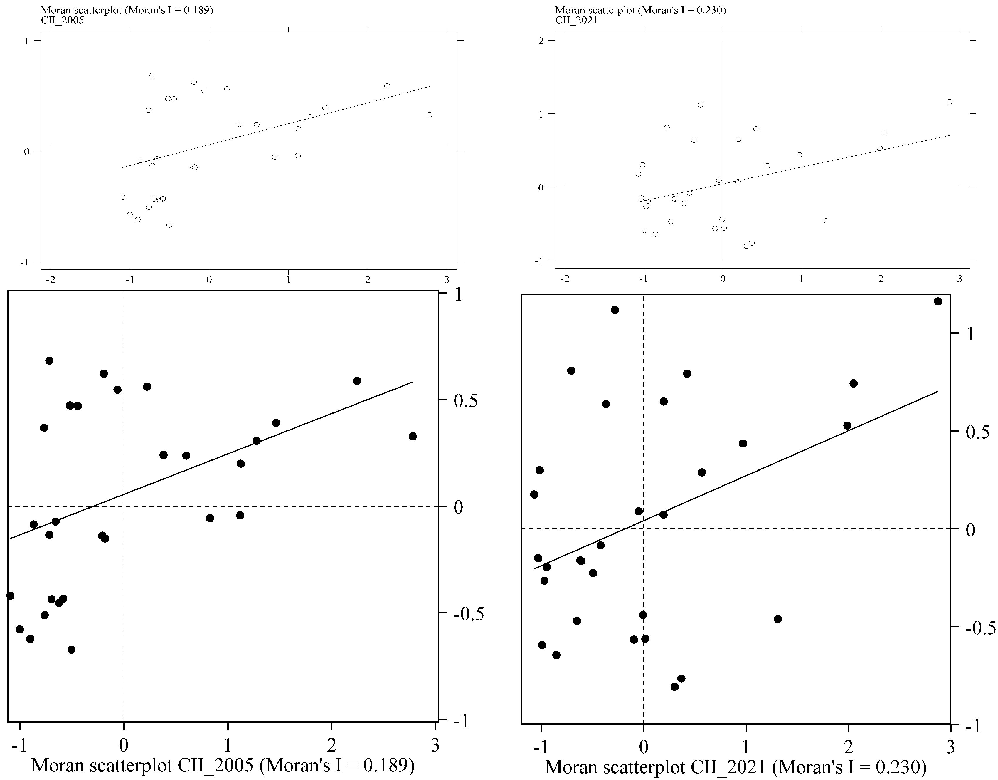
3.3.1. Spatial Autocorrelation Test

Based on the results from

Table 3. Spatial autocorrelation test results of provincial carbon imbalance.

Year	Moran’s I	E (I)	Sd (I)	Z-Value	p-Value
2005	0.189	−0.034	0.121	1.857	0.063
2006	0.212	−0.034	0.120	2.053	0.040
2007	0.259	−0.034	0.120	2.446	0.014
2008	0.288	−0.034	0.120	2.694	0.007
2009	0.275	−0.034	0.120	2.576	0.010
2010	0.294	−0.034	0.120	2.739	0.006
2011	0.303	−0.034	0.121	2.795	0.005
2012	0.316	−0.034	0.119	2.936	0.003
2013	0.312	−0.034	0.121	2.860	0.004
2014	0.278	−0.034	0.121	2.591	0.010
2015	0.272	−0.034	0.120	2.557	0.011
2016	0.290	−0.034	0.119	2.716	0.007
2017	0.261	−0.034	0.121	2.454	0.014
2018	0.237	−0.034	0.120	2.269	0.023
2019	0.243	−0.034	0.119	2.332	0.020
2020	0.234	−0.034	0.120	2.242	0.025
2021	0.230	−0.034	0.120	2.207	0.027

regarding the global spatial autocorrelation and hypothesis testing, it can be observed that Moran’s Index for China’s provincial-level carbon imbalance indices from 2005 to 2021 consistently exceeds 0 and is significant at least at a 10% level. This indicates a positive spatial correlation in the distribution of provincial-level carbon imbalance across China. Specifically, there is evidence of clustering among regions with similar values. This finding significantly supports the inter-regional influence of carbon imbalances among China’s provinces. Moreover, while there is a slight fluctuation in spatial correlation across different years, the overall change remains minimal. This underscores the stability of spatial interactions concerning provincial-level carbon imbalances in China and provides a factual basis for exploring their spatial spillover effects in subsequent sections of this work.

3.3.2. Spatial Agglomeration Characteristics

The Moran scatter plots for China’s provincial-level carbon imbalance indices in 2005 and 2021 are depicted in Figure 2. The horizontal axis represents the standardized carbon imbalance indices for each province, while the vertical axis signifies the spatial lag values of the carbon imbalance indices for each province. It is evident that the majority of provinces fall within the spatially positive correlation regions in quadrants one and three on the scatter plot, with the spatial fit line traversing these quadrants. This indicates that regions with higher carbon imbalance indices tend to have neighboring regions with similarly high carbon imbalance indices, and likewise for regions with lower carbon imbalance indices, suggesting a spatial clustering tendency.

Table 4. Spatial clustering results of carbon imbalance in China.

Features	H-H	L-H	L-L	H-L
Location	First quadrant	Second quadrant	Third quadrant	Fourth quadrant
Correlation	Positive	Negative	Positive	Negative
Properties	Homogeneity	Heterogeneity	Homogeneity	Heterogeneity
2005	Hebei, Shandong, Yunnan	None	Hubei, Chongqing	None
2013	Hebei, Jiangsu, Shandong, Henan	None	Hunan, Chongqing, Gansu	None
2021	Hebei, Jiangsu, Shandong	None	Hunan, Chongqing	None

displays the spatial clustering results of the local Moran indices for the years 2005, 2013, and 2021. In 2005, three provinces—Hebei, Shandong, and Yunnan—were in the “high-high” region. By 2010, Yunnan exited the “high-high” group, while Jiangsu and Henan joined this cluster. In 2021, Henan withdrew from the “high-high” group. The “low-low” cluster primarily includes four provinces: Hubei, Chongqing, Hunan, and Gansu. Hubei left this group in 2013, the same year Hunan and Gansu entered, while Chongqing consistently remained part of this cluster. Furthermore, we observed no discernible “low-high” or “high-low” spatial distribution patterns in China’s provincial-level carbon imbalance. This largely indicates that provincial carbon imbalances exhibit a “prosper together, suffer together” spatial characteristic.

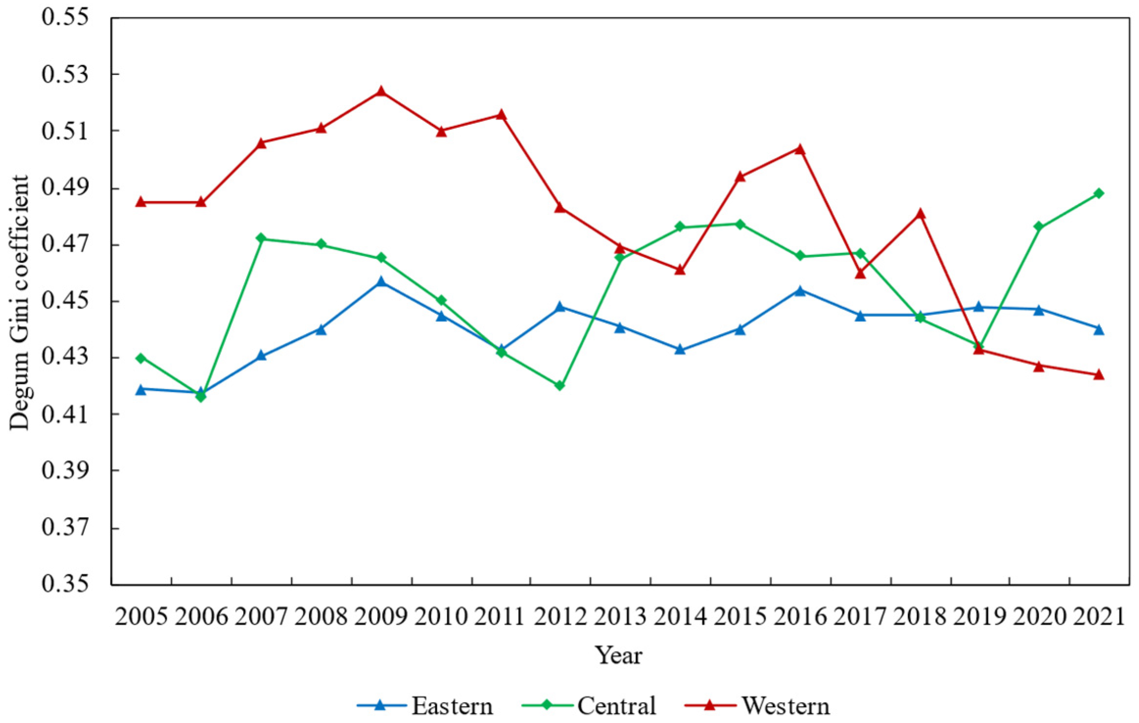
3.3.3. Spatial Gini Coefficient and Decomposition

Table 5. Decomposition results of spatial Gini coefficients.

Year	Gini	Inter-Regional	Rate	Intra-Regional	Rate	Transvariation	Rate
2005	0.461	0.066	14.403	0.155	33.635	0.239	51.961
2006	0.461	0.091	19.680	0.153	33.247	0.217	47.073
2007	0.490	0.117	23.831	0.160	32.632	0.213	43.537
2008	0.496	0.125	25.230	0.162	32.566	0.209	42.204
2009	0.510	0.139	27.326	0.164	32.203	0.206	40.471
2010	0.508	0.190	37.485	0.158	31.149	0.159	31.366
2011	0.504	0.204	40.506	0.154	30.587	0.146	28.907
2012	0.511	0.220	43.059	0.154	30.178	0.137	26.762
2013	0.508	0.195	38.354	0.155	30.510	0.158	31.136
2014	0.503	0.193	38.394	0.154	30.579	0.156	31.028
2015	0.508	0.182	35.779	0.159	31.317	0.167	32.904
2016	0.514	0.185	36.092	0.162	31.474	0.167	32.435
2017	0.496	0.170	34.340	0.156	31.471	0.170	34.189
2018	0.500	0.182	36.462	0.157	31.345	0.161	32.193
2019	0.479	0.161	33.647	0.152	31.828	0.165	34.525
2020	0.485	0.153	31.544	0.154	31.826	0.178	36.630
2021	0.482	0.153	31.788	0.154	31.833	0.175	36.378

presents the results of the decomposition of China’s carbon imbalance based on the Gini coefficient. It is noticeable that after China’s entry into the World Trade Organization, the vast market space led to vigorous economic development. The rapid and robust economic growth brought about substantial carbon emissions. Due to regional resource endowments and geographic disparities, different regions exhibited significant variations in carbon emission levels. Consequently, between 2005 and 2009, there was a continual upward trend in the overall disparity of China’s carbon imbalance.

From 2010 to 2016, China’s economic development shifted from high-speed to moderately high-speed growth, marking the onset of a “new normal” in economic development. As a result, the overall level of disparity in China’s carbon imbalance did not surge rapidly but rather stayed elevated within the range of 0.5 to 0.52. With the deepening of the concept of green development, China’s economy started relying more on technological advancements to propel growth, thus progressing toward green and sustainable development pathways. Consequently, between 2017 and 2021, there was a declining trend in the overall disparity of China’s carbon imbalance. The overall disparity in carbon imbalance among regions gradually reduced. Additionally, the intra-regional disparity in carbon imbalance remained relatively stable at around 0.15 to 0.16, whereas the inter-regional disparity in carbon imbalance exhibited fluctuations. Between 2005 and 2012, it showed an upward trend, reaching its peak at 0.22 in 2012, before declining. Finally, from 2005 to 2010, intra-regional differences played a significant role in causing China’s carbon imbalance, with the contribution rate of intra-regional differences being greater than that of inter-regional differences. However, between 2011 and 2019, this relationship reversed, with inter-regional differences becoming a crucial contributor to China’s carbon imbalance. After 2020, the disparity in carbon imbalance between regions and within regions gradually aligned.

Figure 3 depicts the changing trends in carbon imbalance disparity across China’s eastern, central, and western regions. The variations in carbon imbalance disparity across different regions show distinct characteristics over different periods. Specifically, prior to 2018, the eastern region exhibited relatively lower and stable levels of carbon imbalance disparity compared to the central and western regions. The carbon imbalance disparity in the western and central regions displayed greater fluctuations. Overall, the western region demonstrated a fluctuating downward trend in carbon imbalance disparity after 2009 and became the region with the lowest carbon imbalance disparity after 2019. After 2019, due to differences in economic development and transition among the central regions, the carbon imbalance disparity in the central region gradually widened.

4. Analysis of Influencing Factors of Carbon Imbalance Based on Econometric Model

4.1. Benchmark Regression Results and Comparative Analysis

Table 6. Econometric model regression results.

Variables	Model (1)	Model (2)	Model (3)	Model (4)
	OLS	SLM	SEM	SDM
PS	0.324 *** (0.083)	0.818 *** (0.163)	0.815 *** (0.165)	0.901 *** (0.159)
EG	0.310 *** (0.038)	0.210 *** (0.044)	0.208 *** (0.045)	0.206 *** (0.043)
IS	0.443 (0.296)	0.620 * (0.363)	0.592 (0.363)	1.143 *** (0.364)
EE	−0.266 *** (0.050)	−0.464 *** (0.065)	−0.434 *** (0.069)	−0.292 *** (0.077)
ES	−0.261 (0.339)	0.022 (0.398)	−0.052 (0.413)	−0.551 (0.406)
ρ		0.138 *** (0.050)		0.150 *** (0.050)
λ			0.143 ** (0.059)
Variance sigma2_e		1694.187 *** (106.265)	1698.752 *** (106.614)	1590.600 *** (99.789)
Wald test (SDM→SLM)				32.79 ***
Wald test (SDM→SEM)				39.21 ***
N	510	510	510	510

Notes: ***, **, and * represent significance levels of 1%, 5%, and 10%, respectively; the values in parentheses are standard errors; λ represents the spatial lag coefficient of the error term in SEM.

presents the parameter estimation results for the baseline regression model (OLS) and spatial econometric models (SLM, SEM, and SDM). The results of Model (1), the baseline regression, indicate that the effects of population size, economic growth, and energy efficiency on carbon imbalance are significant, while the industrial structure and electricity structure are not significant contributors to exacerbating carbon imbalance, as their coefficients are not statistically significant. This result suggests that an increase in population size and rapid economic development typically lead to higher energy consumption and production activities, resulting in emissions that intensify carbon imbalance and exacerbate climate change risks. However, the improvement in energy efficiency effectively mitigates the problem of carbon imbalance. This is mainly because the pursuit of higher energy efficiency usually stimulates technological innovation and development, leading to the emergence and application of new energy-saving and clean energy technologies, further reducing dependence on high-carbon energy sources.

It is worth noting that the baseline regression model considers only the average impact effects among variables. However, it is more realistic to acknowledge the presence of some spatial interaction effects in carbon imbalance and economic activities among provinces. This introduces a potential specification bias in the baseline regression model. Therefore, this study further conducts an LM test on the baseline regression model, and the results reject the null hypothesis of the absence of spatial lag and spatial error effects (Spatial error (468.549 ***); Spatial lag (397.932 ***)). Based on this, the study proceeds to construct spatial lag models (SLM), spatial error models (SEM), and spatial Durbin models (SDM) to explore the specific impact effects of different factors on carbon imbalance. The spatial Durbin model, serving as a general spatial model, nests both the spatial lag model and the spatial error model. To examine the validity of the spatial Durbin model specification, a Wald test is employed to conduct a degradation analysis. The test results significantly reject the possibility of SDM degenerating into SLM and SEM at a 1% significance level. Consequently, the subsequent analysis of impact effects will be based on the regression results of model (4).

From the estimation results of model (4), it can be observed that, except for the non-significance of the electricity structure in carbon imbalance, all other variables are statistically significant. This is mainly attributed to the deepening implementation of clean and low-carbon policies. In particular, carbon capture and storage technologies are gradually being adopted in thermal power generation, replacing higher-emission energy sources and effectively mitigating carbon emissions from power plants. An increase in population size, rapid economic growth, and an increase in the proportion of secondary industry exacerbate the issue of carbon imbalance.

On one hand, with population size and economic development, large-scale land use changes and ecosystem disruptions may occur. This may involve deforestation, land development, and urbanization, reducing vegetation coverage and the capacity of natural ecosystems to absorb and store carbon. On the other hand, the increase in population size, rapid economic expansion, and the growing proportion of secondary industry has led to a significant increase in demand for high-carbon fuels, resulting in a substantial increase in carbon emissions. As a result, the decline in carbon sequestration capacity and the increase in carbon emissions ultimately intensify carbon imbalance. However, the innovation of energy-saving and emission-reduction technologies significantly improves energy efficiency, thereby reducing energy consumption. An increase in energy efficiency under the condition of unchanged carbon sequestration capacity will effectively alleviate carbon imbalance. The coefficient of the spatial lag term in the spatial Durbin model is 0.150 and is significant at the 1% level, indicating that carbon imbalance in neighboring regions exacerbates local carbon imbalance, demonstrating a clear spatial spillover effect.

4.2. Effect Decomposition Based on SDM Model

The existence of spatial feedback mechanisms in the spatial Durbin model leads to the inaccurate reflection of the marginal impacts of relevant variables on carbon imbalance. This study draws on the approach proposed by Lesage and Pace (2009) to decompose the direct, indirect, and total effects of various influencing factors. Table 6 presents the results of the effect decomposition of factors influencing carbon imbalance. The direct effects represent the impact of variables on local carbon imbalance, while the indirect effects reveal the influence of variables in neighboring regions on local carbon imbalance. The decomposition of direct effects indicates that population size, economic growth, and industrial structure have significant positive impacts on local carbon imbalance, with industrial structure having the greatest influence, followed by population size, and economic growth last. Conversely, energy efficiency exerts a significantly inhibitory effect on local carbon imbalance (

Table 7. Decomposition results of the impact of various factors on carbon imbalance.

Variables	Direct Effect		Indirect Effect		Total Effect
	Coefficient	Standard Error	Coefficient	Standard Error	Coefficient	Standard Error
PS	0.897 ***	0.160	0.153 ***	0.059	1.051 ***	0.192
EG	0.208 ***	0.044	0.036 **	0.015	0.244 ***	0.052
IS	1.187 ***	0.350	0.206 **	0.100	1.394 ***	0.425
EE	−0.313 ***	0.074	−0.613 ***	0.112	−0.926 ***	0.107
ES	−0.438	0.379	3.560 ***	1.026	3.123 ***	1.051

Notes: ***, **, and * represent significance levels of 1%, 5%, and 10%, respectively.

).

Firstly, in terms of industrial structure, the proportion of the secondary industry’s total output value plays a significant role in promoting carbon imbalance. This is closely related to China’s secondary industry, especially heavy industry, which is characterized by high energy consumption and emissions. Therefore, considering constraints on energy and carbon emissions, a larger share of the secondary industry implies a more serious carbon imbalance. Thus, further greening of the industrial structure undoubtedly becomes one of the key pathways to promote carbon balance. Secondly, rapid economic growth is accompanied by the continued concentration of the population in core urban clusters. The increase in population size usually exhibits characteristics of rigid energy demand and rapid growth in energy consumption. Therefore, population growth is often associated with a resource-intensive and emission-intensive extensive economic growth model. This, in turn, leads to the misuse of land resources, and ecological system destruction, ultimately exacerbating local carbon imbalance.

Thirdly, when regions drive local economies through new and additional material capital investments, repetitive investments aimed solely at expanding reproduction may not only lead to an increase in energy consumption and carbon emissions but also result in overcapacity and the reinforcement of outdated extensive production methods. This hinders the improvement of carbon imbalance. Over the past decade, local governments, in their efforts to stimulate economic growth, have vigorously carried out infrastructure construction and attracted foreign investment, giving rise to an investment boom. This has largely led to inefficient overinvestment and duplication of investments. Excessive and redundant investments result in a rapid increase in energy consumption and carbon emissions. Therefore, economic growth exacerbates local carbon imbalance. Fourthly, the significant improvement in energy efficiency promotes the amelioration of carbon imbalance. The enhancement of energy efficiency signifies technological progress that reduces the energy consumption per unit of GDP. This aligns with the sustainable development concept of promoting energy conservation and emission reduction without sacrificing economic growth, thereby effectively alleviating carbon imbalance. Comparing the parameter estimation results of the spatial Durbin model and the results of direct effect decomposition in the previous sections, slight differences in the values of various variables can be observed. For instance, in the spatial Durbin model, the direct impact coefficient of population size on carbon imbalance is 0.324. In contrast, the direct effect obtained through partial differentiation methods is 0.897. The difference of 0.573 between the two values represents the magnitude of the spatial feedback effect.

According to the results of indirect effect decomposition, all explanatory variables exhibit significant spatial spillover effects. Population size, economic growth, industrial structure, and electricity structure have significant positive impacts on the carbon imbalance in spatially adjacent regions, while energy efficiency has a significant negative impact on the carbon imbalance in spatially adjacent regions. Firstly, due to the evident phenomena of population agglomeration, industrial agglomeration, and economic interdependence among provincial samples, there is a certain degree of convergence in population mobility, industrial structure, and economic adjustments among regions. Therefore, population expansion, economic growth, and the development of secondary industry exacerbate the carbon imbalance in spatially adjacent regions. Secondly, the indirect impact of electricity structure is highly significant, and the increase in the proportion of thermal power locally significantly promotes the carbon imbalance in spatially adjacent regions. Energy consumption is largely influenced by the endowment of energy resources, and adjacent regions often have similar resource endowments, leading to similar energy consumption patterns in neighboring areas. As a result, the adjustment of the electricity structure also shows a certain degree of regional linkage. Additionally, due to the diffusion of carbon emissions and regional air flow, greenhouse gases may intensify carbon imbalance in adjacent regions due to emissions from local thermal power plants. Thirdly, the improvement in energy efficiency affects the carbon emissions and carbon sequestration capacity in spatially adjacent regions through the flow of production factors such as industrial connections, regional cooperation, and labor and capital mobility. This improvement contributes to the carbon imbalance in adjacent regions, representing positive externalities of knowledge and technology.

By comparing the results of the direct and indirect effects, it is observed that the direct effect of electricity structure is not significant, but the indirect effect is significant. In contrast, the direct and indirect effects of population size, economic growth, energy efficiency, and industrial structure are both significant and in the same direction. Therefore, coordinating regional industrial and economic policies with neighboring provinces and cities, and enhancing the exchange and cooperation of technological research and development activities, will be conducive to indirectly promoting the governance of local carbon imbalance. The direct and indirect effects of energy efficiency are both negative, with the indirect effect being greater than the direct effect. This result suggests that improvements in local energy efficiency and technological innovation may impact the carbon imbalance in other regions through mechanisms such as technological spillover. The efforts made by local areas in technology research and development and improving energy efficiency will strengthen the motivation for learning, imitation, and technological improvement in spatially adjacent regions, thereby exerting a greater positive impact on the governance of carbon imbalance in those regions. Moreover, all variables show significant indirect effects, emphasizing the necessity of studying spatial spillover effects in the context of carbon neutrality. The implication is that local governments should avoid unilateral efforts in carbon imbalance governance and, instead, focus on a regional integrated perspective. Based on the concept of a community of shared future, strategic deployments for carbon imbalance governance should be coordinated with neighboring provinces and cities.

4.3. Robustness Test

4.3.1. Eliminate the Influence of Outliers

The presence of extreme values can significantly impact regression results, potentially leading to biased parameter estimates and affecting the accuracy and stability of model estimation. To mitigate the influence of outliers, we conducted a winsorization procedure on the dataset [35]. Extreme values were treated at the 1st and 99th percentiles, with values below 1% set to the 1% value and values above 99% set to the 99% value. Based on the newly processed dataset, a re-estimation was performed using the SDM model.

Table 8. Estimation results after winsorization.

	PS	EG	IS	EE	ES	CII
X	0.901 *** (0.159)	0.206 *** (0.043)	1.143 *** (0.364)	−0.292 *** (0.077)	−0.551 (0.406)
WY						0.150 *** (0.050)
Direct effect	0.897 *** (0.160)	0.208 *** (0.044)	1.187 *** (0.350)	−0.313 *** (0.074)	−0.438 (0.379)
Indirect effect	0.153 *** (0.059)	0.036 ** (0.015)	0.206 ** (0.100)	−0.613 *** (0.112)	3.560 *** (1.026)
Total effect	1.051 *** (0.192)	0.244 *** (0.052)	1.394 *** (0.425)	−0.926 *** (0.107)	3.123 *** (1.051)
Variance sigma2_e	Province	Year	Wald SLM	Wald SEM	R2	N
1590.600 *** (99.789)	FE	FE	32.79 ***	39.21 ***	0.385	510

Notes: ***, **, and * represent significance levels of 1%, 5%, and 10%, respectively; the values in parentheses are standard errors.

reports the new parameter estimates and effect decomposition results. It is observed that the estimated coefficients and impact effects of each factor show no significant differences from the baseline results. This indicates that the baseline regression results are robust under the condition of the entire dataset, even after addressing the influence of outliers through winsorization.

4.3.2. Replace the Spatial Weight Matrix

Considering that the specification of the spatial weight matrix can influence the parameter regression results of the model, we conducted a robustness test using different spatial weight matrices. Given the strong spatial correlation between carbon emissions and the ecological capacity for carbon sequestration [6,36], we employed the widely used spatial weight matrix W_d in spatial econometric analysis for the robustness test. The elements of W_d were set as the reciprocal of the squared geographical distances between provincial capitals. The parameter estimates and effect decomposition results based on W_d are presented in

Table 9. Regression results after replacing the spatial matrix (W_d).

	PS	EG	IS	EE	ES	CII
X	0.890 *** (0.160)	0.178 *** (0.045)	0.791 ** (0.374)	−0.376 *** (0.081)	−0.145 (0.396)
WY						0.256 *** (0.077)
Direct effect	0.893 *** (0.163)	0.182 *** (0.046)	0.840 ** (0.361)	−0.395 *** (0.077)	−0.021 (0.379)
Indirect effect	0.300 ** (0.129)	0.059 ** (0.025)	0.278 * (0.159)	−0.496 ** (0.193)	3.417 ** (1.552)
Total effect	1.193 *** (0.255)	0.241 *** (0.060)	1.118 ** (0.489)	−0.891 *** (0.175)	3.396 ** (1.645)
Variance sigma2_e	Province	Year	Wald SLM	Wald SEM	R2	N
1647.184 *** (103.839)	FE	FE	7.19 **	9.98 ***	0.361	510

Notes: ***, **, and * represent significance levels of 1%, 5%, and 10%, respectively; the values in parentheses are standard errors.

. Firstly, the coefficient of the spatial lag term WY is significantly positive, reaffirming the spatial clustering characteristics of carbon imbalance indices among neighboring provinces. Secondly, the Wald test results reject the possibility of model degeneracy in the SDM model, indicating the validity of the spatial Durbin model set in the earlier sections. Thirdly, comparing the effect decomposition results of the robustness test with the baseline model, it is observed that the impact directions of various factors on carbon imbalance are consistent, and the differences in significance are minor. This suggests that the baseline model results are robust.

4.3.3. Change Parameter Estimation Method

If the number of spatial units is not sufficiently large, employing the Maximum Likelihood Estimation (MLE) method to estimate a spatial panel model with both individual and time-fixed effects may result in inconsistent parameter estimates [37]. To address these issues, the study in [38] proposed the Quasi-Maximum Likelihood Estimation (QMLE) method, providing an operational tool for testing the robustness of our model. This method eliminates individual and time effects, mitigating the adverse interference of the aforementioned problems on parameter estimation, and thereby obtaining consistent estimates for all relevant coefficients.

Table 10. Regression results after changing the estimation method (QMLE).

	PS	EG	IS	EE	ES	CII
X	0.901 *** (0.164)	0.206 *** (0.044)	1.143 *** (0.375)	−0.292 *** (0.079)	−0.551 (0.418)
WY						0.150 *** (0.051)
Direct effect	0.897 *** (0.165)	0.209 *** (0.045)	1.189 *** (0.361)	−0.314 *** (0.076)	−0.437 (0.395)
Indirect effect	0.154 ** (0.069)	0.036 ** (0.016)	0.209 * (0.115)	−0.622 *** (0.123)	3.594 *** (1.006)
Total effect	1.051 *** (0.202)	0.244 *** (0.054)	1.397 *** (0.445)	−0.935 *** (0.117)	3.157 *** (1.048)
Variance sigma2_e	Province	Year	Wald SLM	Wald SEM	R2	N
1689.611 *** (109.250)	FE	FE	30.87 ***	36.92 ***	0.416	480

Notes: ***, **, and * represent significance levels of 1%, 5%, and 10%, respectively; the values in parentheses are standard errors.

reports the SDM estimates and decomposition results using the QMLE method. Both the estimated parameters and effect decomposition results show little difference from the baseline regression results. Moreover, all model tests are statistically significant, reaffirming the robustness of the earlier baseline regression results.

5. Conclusions and Policy Implications

We created a Carbon Imbalance Index for Chinese provinces by combining data on how much carbon dioxide they emit and absorb. We analyzed this data over time and across different regions to understand how carbon imbalance varies both temporally and spatially. Our approach was based on the IPAT framework, and used data from 2005 to 2021 for 30 provinces to achieve this. We developed a spatial Durbin model to investigate what factors influence carbon imbalance. This model helped us examine how the size of the population, the rate of economic growth, the type of industries prevalent, the energy efficiency, and the sources of electricity affect how much carbon imbalance there is in a province. Our main findings are concerning. First, the imbalance between carbon emissions and absorption in Chinese provinces is getting worse over time. Second, this imbalance is not random. Third, the way this imbalance contributes to regional inequality in carbon emissions changes over time. And fourth, factors like increasing population, economic development, growth in secondary industries like manufacturing, and the use of coal for power are making this imbalance worse. However, we also found that improving energy efficiency can help reduce it. Based on these findings, we recommend several strategies for Chinese provinces to address this growing carbon imbalance.

Firstly, our research has found a regional disparity in carbon balance across China. The northeastern and western provinces generally have a carbon surplus due to their lower levels of economic development and a smaller gap between their carbon emissions and the natural carbon sequestration capacity of their ecosystems. This situation results in less pressure for these regions to reduce carbon dioxide emissions. Consequently, these less developed areas can focus on a development model that simultaneously considers economic growth and emission reduction. In contrast, the central and eastern regions of China, which are more economically developed, face greater challenges with carbon deficits, primarily due to higher carbon emissions exceeding their ecosystems’ absorption capacities. For these regions, a different approach is needed. They should adopt strategies that focus on stabilizing their economies while aggressively pursuing emission reduction. This involves integrating sustainable practices into their economic growth models to address the pressing need for environmental responsibility. Therefore, our recommendation is for regional government authorities to devise development strategies that are tailored to their unique environmental and economic contexts, emphasizing green and sustainable development while considering the distinct characteristics of each region.

Secondly, we reveal a significant spatial positive correlation in carbon imbalance across Chinese provinces, which essentially means that regions tend to experience similar trends in carbon imbalance. When one region prospers or struggles in terms of carbon balance, neighboring regions tend to follow a similar pattern. This discovery highlights the importance of considering regional interactions when addressing carbon imbalance issues. To effectively tackle this challenge at the provincial level in China, a comprehensive, nationwide approach is essential. It is important to recognize and address the interconnected nature of carbon imbalances across different regions, making use of the ‘spatial spillover effects’ where actions in one region can impact others. This approach requires breaking down regional barriers, fostering cooperation across provinces, and establishing a coordinated strategy for both reducing carbon emissions and enhancing ecological quality. Additionally, the strategy should focus on implementing and executing a development philosophy centered on ecological civilization, which involves creating a cohesive plan for regional carbon reduction and ecosystem protection. Moreover, it is crucial to address the spatial inequalities in carbon imbalance and work towards minimizing the disparities in carbon balance across different regions. This approach calls for a balanced combination of local and national efforts to ensure a harmonious and sustainable environmental future.

Finally, after evaluating the factors contributing to carbon imbalance and their spatial effects, we propose several policy recommendations to tackle this complex issue. (1) To address the carbon emissions and environmental challenges stemming from population growth, we suggest enhancing public awareness about energy conservation and emission reduction. Encouraging people to adopt a green, low-carbon lifestyle is essential. (2) We recommend the promotion of green taxation and subsidy policies. These policies could incentivize businesses to embrace more eco-friendly and sustainable production practices. We also advocate for the advancement of a circular economy by increasing the recycling and reuse of resources, which would help in reducing waste. (3) It is crucial to use policy support, funding, and technological innovation to transform industries with high carbon footprints into low-carbon and clean operations. (4) Establishing and enforcing more stringent energy efficiency standards could stimulate businesses to invest in green technology research and development. This approach should include promoting the regional use and spread of green patents and encouraging both businesses and households to use more energy-efficient technologies and equipment. (5) We recommend a gradual shift in the electricity sector from traditional, high-carbon energy sources to cleaner alternatives like solar, wind, and hydropower. Taken together, these recommendations aim to address various aspects of carbon imbalance through a range of strategies, each contributing to a comprehensive approach to mitigate this pressing environmental challenge.

References

1. Sun, P.; Zhai, S.; Chen, J.; Yuan, J.; Wu, Z.; Weng, X. Development of a multi-active center catalyst in mediating the catalytic destruction of chloroaromatic pollutants: A combined experimental and theoretical study. Appl. Catal. B Environ. 2020, 272, 119015. [Google Scholar] [CrossRef]
2. Cheng, L.; Li, Y.; Fan, J.; Xie, M.; Liu, X.; Sun, P.; Dong, X. High efficiency photothermal synergistic degradation of toluene achieved through the utilization of a nickel foam loaded Pt-CeO2 monolithic catalyst. Sep. Purif. Technol. 2024, 333, 125742. [Google Scholar] [CrossRef]
3. Chen, L.; Xu, L.; Cai, Y.; Yang, Z. Spatiotemporal patterns of industrial carbon emissions at the city level. Resour. Conserv. Recycl. 2021, 169, 105499. [Google Scholar] [CrossRef]
4. Gui, D.; He, H.; Liu, C.; Han, S. Spatio-temporal dynamic evolution of carbon emissions from land use change in Guangdong Province, China 2000–2020. Ecol. Indic. 2023, 156, 111131. [Google Scholar] [CrossRef]
5. Wang, M.; Wang, Y.; Teng, F.; Ji, Y. The spatiotemporal evolution and impact mechanism of energy consumption carbon emissions in China from 2010 to 2020 by integrating multisource remote sensing data. J. Environ. Manag. 2023, 346, 119054. [Google Scholar] [CrossRef] [PubMed]
6. Zhou, K.; Yang, J.; Yang, T.; Ding, T. Spatial and temporal evolution characteristics and spillover effects of China’s regional carbon emissions. J. Environ. Manag. 2023, 325, 116423. [Google Scholar] [CrossRef]
7. Zhang, W.; Liu, X.; Wang, D.; Zhou, J. Digital economy and carbon emission performance: Evidence at China’s city level. Energy Policy 2022, 165, 112927. [Google Scholar] [CrossRef]
8. Wen, S.; Liu, H. Research on energy conservation and carbon emission reduction effects and mechanism: Quasi-experimental evidence from China. Energy Policy 2022, 169, 113180. [Google Scholar] [CrossRef]
9. Wang, Z.; Zhang, J.; Luo, P.; Sun, D.; Li, J. Revealing the spatio-temporal characteristics and impact mechanism of carbon emission in China’s urban agglomerations. Urban Clim. 2023, 52, 101733. [Google Scholar] [CrossRef]
10. Yu, Z.; Khan, S.A.R.; Ponce, P.; de Sousa Jabbour, A.B.L.; Jabbour, C.J.C. Factors affecting carbon emissions in emerging economies in the context of a green recovery: Implications for sustainable development goals. Technol. Forecast. Soc. Chang. 2022, 176, 121417. [Google Scholar] [CrossRef]
11. Benlemlih, M.; Assaf, C.; El Ouadghiri, I. Do political and social factors affect carbon emissions? Evidence from international data. Appl. Econ. 2022, 54, 6022–6035. [Google Scholar] [CrossRef]
12. Li, A.; Zhang, A.; Zhou, Y.; Yao, X. Decomposition analysis of factors affecting carbon dioxide emissions across provinces in China. J. Clean. Prod. 2017, 141, 1428–1444. [Google Scholar] [CrossRef]
13. Xu, B.; Lin, B. Factors affecting carbon dioxide (CO2) emissions in China’s transport sector: A dynamic nonparametric additive regression model. J. Clean. Prod. 2015, 101, 311–322. [Google Scholar] [CrossRef]
14. Jiang, Y.; Lei, Y.L.; Yang, Y.Z.; Wang, F. Factors affecting the pilot trading market of carbon emissions in China. Pet. Sci. 2018, 15, 412–420. [Google Scholar] [CrossRef]
15. Lin, B.; Xu, B. Factors affecting CO2 emissions in China’s agriculture sector: A quantile regression. Renew. Sustain. Energy Rev. 2018, 94, 15–27. [Google Scholar] [CrossRef]
16. Xu, G.; Zhao, T.; Wang, R. Decomposition and decoupling analysis of factors affecting carbon emissions in China’s regional logistics industry. Sustainability 2022, 14, 6061. [Google Scholar] [CrossRef]
17. Duman, Z.; Mao, X.; Cai, B.; Zhang, Q.; Chen, Y.; Gao, Y.; Guo, Z. Exploring the spatiotemporal pattern evolution of carbon emissions and air pollution in Chinese cities. J. Environ. Manag. 2023, 345, 118870. [Google Scholar] [CrossRef] [PubMed]
18. Lal, R. Soil carbon sequestration impacts on global climate change and food security. Science 2004, 304, 1623–1627. [Google Scholar] [CrossRef] [PubMed]
19. McFarland, J.R.; Herzog, H.J. Incorporating carbon capture and storage technologies in integrated assessment models. Energy Econ. 2006, 28, 632–652. [Google Scholar] [CrossRef]
20. Wei, X.; Yang, J.; Luo, P.; Lin, L.; Lin, K.; Guan, J. Assessment of the variation and influencing factors of vegetation NPP and carbon sink capacity under different natural conditions. Ecol. Indic. 2022, 138, 108834. [Google Scholar] [CrossRef]
21. Liu, Z.; Wang, W.; Chen, Y.; Wang, L.; Guo, Z.; Yang, X.; Yan, J. Solar harvest: Enhancing carbon sequestration and energy efficiency in solar greenhouses with PVT and GSHP systems. Renew. Energy 2023, 211, 112–125. [Google Scholar] [CrossRef]
22. He, Y.; Ren, Y. Can carbon sink insurance and financial subsidies improve the carbon sequestration capacity of forestry? J. Clean. Prod. 2023, 397, 136618. [Google Scholar] [CrossRef]
23. Lyu, J.; Fu, X.; Lu, C.; Zhang, Y.; Luo, P.; Guo, P.; Zhou, M. Quantitative assessment of spatiotemporal dynamics in vegetation NPP, NEP and carbon sink capacity in the Weihe River Basin from 2001 to 2020. J. Clean. Prod. 2023, 428, 139384. [Google Scholar] [CrossRef]
24. Ehrlich, P.R.; Holdren, J.P. Impact of Population Growth: Complacency concerning this component of man’s predicament is unjustified and counterproductive. Science 1971, 171, 1212–1217. [Google Scholar] [CrossRef]
25. York, R.; Rosa, E.A.; Dietz, T. Bridging environmental science with environmental policy: Plasticity of population, affluence, and technology. Soc. Sci. Q. 2002, 83, 18–34. [Google Scholar] [CrossRef]
26. LeSage, J.; Pace, R.K. Introduction to Spatial Econometrics; Chapman and Hall/CRC: London, UK, 2009. [Google Scholar]
27. Chen, J.; Fan, W.; Li, D.; Liu, X.; Song, M. Driving factors of global carbon footprint pressure: Based on vegetation carbon sequestration. Appl. Energy 2020, 267, 114914. [Google Scholar] [CrossRef]
28. Li, M.; Liu, H.; Geng, G.; Hong, C.; Liu, F.; Song, Y.; Tong, D.; Zheng, B.; Cui, H.; Man, H.; et al. Anthropogenic emission inventories in China: A review. Natl. Sci. Rev. 2017, 4, 834–866. [Google Scholar] [CrossRef]
29. Zheng, B.; Tong, D.; Li, M.; Liu, F.; Hong, C.; Geng, G.; Li, H.; Li, X.; Peng, L.; Qi, J.; et al. Trends in China’s anthropogenic emissions since 2010 as the consequence of clean air actions. Atmos. Chem. Phys. 2018, 18, 14095–14111. [Google Scholar] [CrossRef]
30. Shi, K.; Liu, G.; Cui, Y.; Wu, Y. What urban spatial structure is more conducive to reducing carbon emissions? A conditional effect of population size. Appl. Geogr. 2023, 151, 102855. [Google Scholar] [CrossRef]
31. Li, B.; Haneklaus, N. Reducing CO2 emissions in G7 countries: The role of clean energy consumption, trade openness and urbanization. Energy Rep. 2022, 8, 704–713. [Google Scholar] [CrossRef]
32. Zheng, H.; Gao, X.; Sun, Q.; Han, X.; Wang, Z. The impact of regional industrial structure differences on carbon emission differences in China: An evolutionary perspective. J. Clean. Prod. 2020, 257, 120506. [Google Scholar] [CrossRef]
33. Deka, A.; Bako, S.Y.; Ozdeser, H.; Seraj, M. The impact of energy efficiency in reducing environmental degradation: Does renewable energy and forest resources matter? Environ. Sci. Pollut. Res. 2023, 30, 86957–86972. [Google Scholar] [CrossRef] [PubMed]
34. Fan, G.; Zhu, A.; Xu, H. Analysis of the Impact of Industrial Structure Upgrading and Energy Structure Optimization on Carbon Emission Reduction. Sustainability 2023, 15, 3489. [Google Scholar] [CrossRef]
35. Cheng, X.; Yao, D.; Qian, Y.; Wang, B.; Zhang, D. How does fintech influence carbon emissions: Evidence from China’s prefecture-level cities. Int. Rev. Financ. Anal. 2023, 87, 102655. [Google Scholar] [CrossRef]
36. Zhao, N.; Wang, K.; Yuan, Y. Toward the carbon neutrality: Forest carbon sinks and its spatial spillover effect in China. Ecol. Econ. 2023, 209, 107837. [Google Scholar] [CrossRef]
37. Chai, J.; Tian, L.; Jia, R. New energy demonstration city, spatial spillover and carbon emission efficiency: Evidence from China’s quasi-natural experiment. Energy Policy 2023, 173, 113389. [Google Scholar] [CrossRef]
38. Lee, L.F.; Yu, J. Estimation of spatial autoregressive panel data models with fixed effects. J. Econom. 2010, 154, 165–185. [Google Scholar] [CrossRef]
Figure 1. KDE result of provincial carbon imbalance.
Sustainability 16 01805 g001
Figure 2. Moran scatter plot of provincial carbon imbalance.
Sustainability 16 01805 g002
Figure 3. Dagum’s Gini coefficient change trend of regional carbon imbalance.
Sustainability 16 01805 g003