Advanced Integration of Forecasting Models for Sustainable Load Prediction in Large-Scale Power Systems

Abstract

In the burgeoning field of sustainable energy, this research introduces a novel approach to accurate medium- and long-term load forecasting in large-scale power systems, a critical component for optimizing energy distribution and reducing environmental impacts. This study breaks new ground by integrating Causal Convolutional Neural Networks (Causal CNN) and Variational Autoencoders (VAE), among other advanced forecasting models, surpassing conventional methodologies in this domain. Methodologically, the power of these cutting-edge models is harnessed to assimilate and analyze a wide array of influential factors, including economic trends, demographic shifts, and natural phenomena. This approach enables a more nuanced and comprehensive understanding of power load dynamics, essential for accurate forecasting. The results demonstrate a remarkable improvement in forecasting accuracy, with a 15% increase in precision over traditional models. Additionally, the robustness of the forecasting under varying conditions showcases a significant advancement in predicting power loads more reliably. In conclusion, the findings not only contribute substantially to the field of load forecasting but also highlight the pivotal role of innovative methodologies in promoting sustainable energy practices. This work establishes a foundational framework for future research in sustainable energy systems, addressing the immediate challenges and exploring potential future avenues in large-scale power system management.

1. Introduction

In the realm of regional infrastructure development, the planning and construction of electric grids hold a critical role. This research is dedicated to augmenting the role of power grids in bolstering regional and economic advancement, with a pronounced focus on the societal and environmental benefits accruing to electricity consumers. It tackles the imperative challenge of maintaining a reliable and secure electricity supply within expansive power systems, a fundamental pillar in the evolution of grid infrastructure [1]. The adoption of modern technological solutions in grid planning and construction is indispensable for aligning with national unified power system standards, thereby ensuring grid stability and safety, while simultaneously promoting accelerated development.

The cornerstone of effective grid planning lies in precise load forecasting and power demand analysis. These elements are pivotal in providing necessary support for investment strategies and have a profound influence on the long-term developmental trajectory of power systems. This study underscores the significance of medium- to long-term load forecasting in large-scale power systems. Such forecasting is instrumental in guiding the strategic positioning and specifications of substations and plays a vital role in furnishing indispensable data for project authorization processes. In the context of heightened global environmental consciousness, the accuracy of long-term load forecasting becomes increasingly vital for the stability of power systems [2]. While traditional forecasting methodologies have their limitations, they are now being effectively supplemented by the emerging advancements in deep learning technologies.

The study introduces a novel integration of Deep Causal Convolutional Neural Networks (Causal CNN) and Variational Autoencoders (VAE), named VAE-CCNN. This model utilizes Causal CNN to analyze sequential and causal relationships in power load data, while VAE addresses complex probability distributions, shedding light on the nonlinear and uncertain characteristics of power loads in large-scale systems. This approach significantly enhances the accuracy of medium- to long-term load forecasting in large-scale power systems, providing invaluable insights for grid planning and ensuring stable operation.

In the context of integrating Causal Convolutional Neural Networks (Causal CNN) and Variational Autoencoders (VAE) for enhanced forecasting in large-scale power systems, a review of the current literature reveals significant advancements in the field. The application of deep learning and machine learning techniques in electric load forecasting is increasingly prominent, with studies exploring various innovative approaches and methodologies.

In the field of building energy load forecasting, researchers such as Katsatos and Moustris [1], Gao et al. [2], and Barzola-Monteses et al. [3] primarily focus on understanding demand-side management in electric load forecasting. Their research emphasizes the critical role of various external factors such as HVAC systems, automated lighting solutions, and occupancy patterns, which are crucial for accurately predicting the energy loads in public and office buildings.

In the advancement of predictive modeling, Shu, X. et al. (2021) demonstrated significant progress in their study “VAE-TALSTM: A Temporal Attention and Variational Autoencoder-based Long Short-Term Memory Framework for Dam Displacement Prediction” [4]. This research introduced an innovative predictive model combining Variational Autoencoders (VAE) and Temporal Attention-based Long Short-Term Memory networks (TALSTM) for predicting long-term deformations in arch dams. Ingeniously integrating a CNN-based VAE for extracting features from environmental data and a TALSTM for establishing the relationship between dam displacement and these extracted features, this study showcased its stability and effectiveness over nine baseline prediction models in the crucial field of dam health monitoring. Their approach to leveraging advanced neural network architectures for enhancing prediction accuracy provides valuable insights for this study, especially in the context of improving the predictive capability of complex systems through temporal attention mechanisms.

In the realm of renewable energy, the study by Jlidi, M. et al. (2023), “An Artificial Neural Network for Solar Energy Prediction and Control Using Jaya-SMC”, is equally noteworthy [5]. The paper delved into the use of Artificial Neural Networks (ANNs) for predicting the performance of photovoltaic systems under various meteorological conditions, employing a hybrid control approach combining the JAYA algorithm and Sliding Mode Control (SMC). Their methodology, utilizing extensive datasets for predicting temperature and solar radiation impacts on photovoltaic systems, achieved high accuracy and robustness, with a regression value of 0.971 and a mean squared error of 0.003. The emphasis of this research on the impact of predictive analytics on energy efficiency and photovoltaic system control underscores the growing importance of forecasting in renewable energy technologies. Their discussed predictive approaches and control strategies resonate with this study’s focus on enhancing the accuracy and efficiency of energy system predictions, thus contributing to a more comprehensive understanding of advanced neural network applications in energy forecasting and management.

In the context of grid control and demand-side management within smart grids, the research by Chan et al. [6], Shikulskaya et al. [7], and Krishnan et al. [8] underscores the importance of precise grid load forecasting for more effective energy scheduling and identifying potential volatile areas in the electricity network, thus improving its operational quality. This is especially relevant in large-scale power systems, where accurate forecasting is critical for ensuring grid stability and efficiency.

With the evolution of various neural networks, many studies integrate these networks (often in conjunction with traditional methods such as ARIMA) to achieve higher accuracy in load forecasting. In this regard, the works of Krishnan et al. [8], Rosato et al. [9,10], and Qi et al. [11] stand out as particularly noteworthy. These models, especially those that combine CNN and LSTM networks, achieve significant success due to their ability to automatically learn features and effectively process time series data.

Moreover, the application of these advanced forecasting techniques extends beyond traditional power system environments. For instance, research by Pramono et al. [12] and Kim & Cho [13] demonstrates the adaptability of these models across various contexts, from individual households to entire grids, indicating the vast potential of these techniques in enhancing load forecasting in large-scale power systems.

In summary, the current state of research in electric load forecasting, especially with the integration of advanced deep learning techniques such as Causal CNN and VAE, indicates a promising trajectory towards more accurate, efficient, and robust forecasting models. These advancements not only contribute significantly to the theoretical understanding of load forecasting but also have practical implications for the planning and operation of large-scale power systems [14]. In the context of medium- to long-term electric load forecasting for large-scale power systems, a comprehensive approach is required, which begins with analyzing influencing factors and then employing advanced techniques such as deep learning for prediction [15]. The term “medium- to long-term” is often not explicitly defined in most studies but is generally considered to span nearly a decade.

In this study, the emphasis is placed on medium- to long-term forecasting for large-scale power systems, leveraging advanced deep learning technologies to increase the precision and stability of the predictions. It is critical to take into account the entire lifecycle of power equipment, as it dictates the period of forecasting. Adopting a full lifecycle perspective involves consideration of the entire duration, starting from the design phase, particularly in the power sector, to ensure that the forecasts are in line with the operational lifespan of the equipment. This alignment is essential to avoid overloading and premature retirement of the equipment, thereby averting cost inefficiencies.

From a cost perspective, the total lifecycle cost of equipment includes investment, operation and maintenance, outage losses, and recycling costs. Over time, as the total lifecycle cost increases, the economic efficiency decreases. Researchers such as Bai [16] have used system dynamics models to study grid costs and proposed cost optimization models. Additionally, considering the physical lifespan of different components, such as transformers and cables, is essential. The lifespans of these components are typically determined through statistics and experimentation. In 2012, the State Grid Corporation of China set standards for the physical service life of grid equipment. Therefore, in medium- to long-term forecasting for large-scale power systems, it is imperative to comprehensively consider both economic and physical lifespans to ensure that predictions are both scientific and practical.

This approach underscores the importance of integrating advanced forecasting techniques with a deep understanding of the operational and economic aspects of power systems, ensuring that the predictions not only leverage the latest in technology but are also grounded in the practical realities of power system management. The remainder of this manuscript is systematically organized to facilitate a coherent and in-depth understanding of this research. Section 2 critically examines the existing literature, delineating the current state-of-the-art methodologies and identifying gaps that this study aims to address. Section 3 articulates the conceptual framework and detailed structure of the proposed VAE-CCNN model, underscoring its innovative aspects. Section 4 delineates the methodological approach, encompassing data acquisition, model implementation, and evaluation metrics. The empirical results and their analytical interpretation are presented later, highlighting the efficacy and practical implications of the model. Finally, Section 5 synthesizes the research outcomes, discusses their broader implications for sustainable energy systems, and proposes directions for future research endeavors.

2. Materials and Methods

2.1. Electricity Load Evaluation Function

In the realm of large-scale power systems, forecasting the electricity load over medium- to long-term horizons necessitates a nuanced approach. While academically similar to conventional “medium- to long-term electric load forecasting”, the methodology diverges fundamentally by incorporating an in-depth analysis of influencing factors to enhance forecast precision.

Traditionally, methods such as absolute error, squared error sum, mean absolute error, and root mean square error have been employed for forecast assessment. These methods effectively reveal discrepancies between predicted and actual values over different periods, thus serving as indicators of forecast quality. However, such evaluation mechanisms often overlook the varying significance of errors across short and long-term forecasts and tend to equate errors in absolute terms, which may not be conducive to in-depth comparative analysis of forecasting strategies [17].

To address this, the error computation assigns greater weight to errors in medium- to long-term forecasts. In the context of long-term forecasting, overestimation can lead to increased initial investment and selection of overly capable equipment, resulting in unnecessary wastage and cost losses. Conversely, underestimation could escalate maintenance costs and potentially truncate the project lifecycle prematurely.

2.1.1. Time-Dimensional Forecast Error Evaluation Function

Acknowledging the challenges in accurately predicting long-term unit energy consumption—which may decline slightly over time yet is harder to forecast—compared to the relative ease in early-stage predictions [18], the accepted principle is that long-term forecast accuracy should supersede short-term accuracy. This leads us to propose a time-dimensional error evaluation function, formulated as follows:

$$E={\displaystyle \sum }_{n=1}^k{e}^{\frac{n}{k}}\frac{\left|y_k-S_k\right|}{S_k}$$

(1)

where E represents the evaluation function; n is the difference in years between forecasted and known data; k denotes the maximum forecast year; $S_k$ is the actual value in the kth year; and $y_k$ is the forecasted value in the kth year.

2.1.2. Forecast Error Evaluation Function for Lifecycle Cost Considerations

As previously mentioned, the total lifecycle cost of electrical equipment encompasses four components. Long-term forecast errors can impact initial investments and the overall lifespan of the electricity grid [19]. Studies indicate that forecast data in the final year of the prediction period significantly influence equipment selection decisions. Overestimations spread the cost across the entire lifespan of the equipment, while underestimations can shorten the overall project life, increasing annual costs [20]. From an energy conservation and emission reduction perspective, the evaluation function differentiates between overestimations and underestimations, as proposed in the following formulation:

$$\left\{\begin{array}{c}E=\frac{y_k-s_k}{y_{n}k},y_k-s_k>=0\\ E=\frac{y_k-s_k}{s_{k}k},y_k-s_k<0\end{array}\right.$$

(2)

By integrating these two evaluation functions, a comprehensive framework is established to assess electricity load forecasts in large-scale power systems, ensuring that the predictions are both scientifically rigorous and practically viable.

$$\left\{\begin{array}{c}E={{\displaystyle \sum }}_{n=1}^{k-1}{e}^{\frac{n}{k}}\frac{\left|y_n-s_n\right|}{s_n}+e\frac{y_k-s_k}{y_{n}k},y_k-s_k>=0\\ E={{\displaystyle \sum }}_{n=1}^{k-1}{e}^{\frac{n}{k}}\frac{\left|y_n-s_n\right|}{s_n}+e\frac{s_k-y_k}{s_{k}k},y_k-s_k<0\end{array}\right.$$

(3)

2.2. Methods of Load Forecasting

The “long-term forecast horizon” referred to in this study is understood as the period during which major updates to the power grid’s main equipment are not required, nor is there a need for large-scale re-planning of the power grid. In accordance with the standards of power grid and national power grid planning, the electricity load forecast for Rudong County is set for a 15-year period, projecting up to the year 2035.

Given the extended duration of long-term power load forecasting, traditional methods such as regression analysis and per capita consumption methods may yield significant errors and be susceptible to various interfering factors, thus rendering them unsuitable for such long-term predictions.

A review of the existing literature suggests that a tiered and layered approach to long-term electric load forecasting can enhance accuracy. Accordingly, this study utilizes the spatial load density method, an optimized gray forecasting model, and the VAE-CCNN model for prediction. The results from these models are then amalgamated using the Ordered Weighted Averaging (OWA) operator to forecast the electricity demand of Rudong County in 2035.

This approach aligns with the advancements in the field, as highlighted by studies such as Aguiar et al. [21] and Sharma et al. [22], which emphasize the importance of integrating various forecasting methods to enhance prediction accuracy in large-scale power systems.

2.2.1. Spatial Load Density Forecasting

In the domain of urban development and planning, spatial load density forecasting stands as a mainstream method within hierarchical forecasting techniques, particularly favored for its effectiveness. This method subdivides the forecasting area into different functional land uses, such as residential, commercial, industrial, storage, transportation, public facilities, and green spaces. This segmentation facilitates precise predictions of saturated loads. The forecasting load is calculated using the following formula: Load = Constructed Land Area × Floor Area Ratio × Building Load Density × Coincidence Factor. Building load density and the coincidence factor are crucial parameters in this calculation. Building load density is often derived from user survey data and can reference standards such as the Urban Electric Power Planning Specification (GB/T50293-2014) [23]. The core of using the load density method for predicting transitional year load lies in determining the transitional year load density indicator [24].

Given the finite nature of urban space, load density cannot grow indefinitely; its rate of increase tends to slow over time, typically represented by an S-shaped curve.

$$y_t=\frac{k}{1+e^{-rt+c}}$$

(4)

The coincidence factor delineates the relationship between the grid’s maximum load and the sum of the maximum loads of all users, reflecting the probability of maximum power usage by users at any given moment. This indicator is closely related to socio-economic conditions and seasonal factors. In practice, it can be estimated using empirical methods or by superimposing typical daily load curves. The specific forecasting steps are as follows:

Aggregate the area of each type of land use according to urban planning, select appropriate load density indicators, and calculate the predicted load value.

Collect hourly load data on a typical day to plot the daily load curve.

Integrate the daily load curves of different land uses with the predicted load values to obtain the region’s coincidence rate.

The specific algorithm is as follows:

$$t=\frac{P_A{t}_A}{{{\displaystyle \sum }}_n{P}_{An}^{\prime }}=\frac{{{\displaystyle \sum }}_n{P}_A{t}_A}{{{\displaystyle \sum }}_n{P}_{An}{t}_{An}}$$

(5)

where $P_A$ represents the load of grid $A$ without considering the coincidence factor of the supply unit level; $P_{An}$ is the load of the supply unit $An$ without considering its internal coincidence factor; $P_{An}^{\prime }$ is the load of the supply unit $An$ considering its internal coincidence factor; $t_{An}$ is the coincidence factor of grid $A$ without considering the supply unit level (which can be superimposed using the daily load characteristic curve); and $t_{An}$ is the coincidence factor of the supply unit $An$. Historically, in grid-based planning and load forecasting processes, there was no explicit method for selecting the inter-unit coincidence factor, only a general range of 0.95 to 1.

This approach to spatial load density forecasting is critical in the context of large-scale power systems, as it allows for a more nuanced understanding of load patterns, incorporating advances in urban planning and power grid optimization. The integration of such sophisticated methods is essential for enhancing the accuracy and reliability of long-term load forecasts, aligning with the overall theme of integrating advanced technologies such as Causal CNN and VAE in power system forecasting. This methodological framework not only contributes to the theoretical advancement in the field but also has practical implications for the planning and operation of complex power grids [25].

2.2.2. Gray Forecasting

Gray forecasting is particularly effective in scenarios where the system data is incomplete or uncertain, a common challenge in electric load forecasting [26]. This methodology assumes that even systems with seemingly random behavior exhibit underlying patterns that can be modeled and predicted. In the context of electric load forecasting, this approach is valuable for its ability to make accurate predictions despite the inherent uncertainties and limited data typically associated with energy consumption patterns.

The core of traditional gray forecasting is encapsulated in the GM(1.1) model, a first-order differential equation. Equation (6) represents the whitenization differential equation for this model. In this equation, $\frac{d{X}^{\left(1\right)}}{dt}$ denotes the rate of change in the accumulated series, where $X^{\left(1\right)}$ is the first-order accumulated series derived from the original data $X^{\left(0\right)}$. The terms ‘a’ and ‘b’ in the equation are critical: ‘a’ is the development coefficient indicating the growth rate, whereas ‘b’ represents the gray action quantity, essentially a constant term in the differential equation. These coefficients are calculated using the least squares method, as shown in Equation (7), ensuring that the model closely fits the historical data and improves their predictive accuracy.

$$\frac{d{X}^{\left(1\right)}}{dt}+a{X}^{\left(1\right)}=b$$

(6)

Here, $a$ is the development coefficient, and $b$ is the gray action quantity, solved using the least squares method:

$${[a,b]}^T={\left(B^{T}B\right)}^{-1}{B}^T{Y}_n$$

(7)

In this study, the limitations of the traditional GM(1.1) model, especially for long-term forecasting and scenarios with rapidly changing data, were recognized. To enhance its performance, an optimization in the form of a revised background value was introduced, as presented in Equation (8). This modification involves a smoothing technique, where $z^{\left(1\right)}\left(k+1\right)$ is the adjacent mean generation method, designed to reduce the lag errors in volatile data scenarios. This adjustment is crucial for improving the model’s fitting and predictive efficacy, especially in the complex and dynamic environment of large-scale power system forecasting.

$$z^{\left(1\right)}\left(k+1\right)=\frac{x^{\left(1\right)}\left(k+1\right)-x^{\left(1\right)}\left(k\right)}{\ln x^{\left(1\right)}\left(k+1\right)-\ln x^{\left(1\right)}\left(k\right)}$$

(8)

The enhancements made to the traditional gray forecasting model are in line with the broader approach of incorporating advanced methodologies such as Causal CNN and Variational Autoencoders (VAE). By refining the gray forecasting model and integrating it with these cutting-edge techniques, the aim is to create a more robust and precise forecasting tool. This is particularly important in the context of electric load forecasting for large-scale power systems, where accuracy and the ability to handle complex, uncertain data are paramount.

2.2.3. Deep Causal Convolutional Neural Networks

Deep Causal Convolutional Neural Networks (Causal CNNs) represent a specialized variant of convolutional neural networks, specifically designed to address problems involving explicit time series causal relationships. These networks are particularly effective in fields such as natural language processing, speech recognition, video analysis, and predictive modeling, where the input data has a clear temporal sequence and predictions should be based solely on past data [27]. This design approach helps mitigate the issue of future data “leaking” into the past, a potential problem with standard convolutional neural networks.

The architectural foundation of Causal CNNs is quite similar to traditional convolutional networks, encompassing components such as convolutional layers, nonlinear activation functions, pooling layers, and fully connected layers. The distinctive feature of Causal CNNs lies in their convolution operations, which are strictly confined to past and present points in the time series, deliberately excluding future data. Specifically, during convolution operations with a time series, the convolutional kernel slides only up to the current time point and not into future points, ensuring the causality of the model.

In a scenario where an input sequence $x=\left(x_1,x_2,\dots ,x_T\right)$ and a convolutional kernel of length $L,h=\left(h_1,h_2,\dots ,h_L\right)$, are given, the convolution operation at time $t$ in a Causal CNN can be expressed as

$$y_t=\sum _{\tau =0}^{\infty }{h}_{\tau }{x}_{t-\tau }$$

(9)

Here, $y_t$ is the output at time $t,h_{\tau }$ is the value of the convolutional kernel at position $\mathsf{\tau }$, and $x_{t-\tau }$ is the input at time $t-\tau$. The range of $\tau$ from 0 to infinity ensures that the convolution operation is conducted only on past and present data. However, practically, given the finite length of the convolutional kernel, $h_{\tau }$ equals zero when $\tau$ exceeds the length of the kernel.

In the context of forecasting in large-scale power systems, the Causal CNNs’ ability to maintain the integrity of temporal data is crucial. This characteristic aligns with the theme of integrating advanced predictive models, such as Causal CNNs and VAE, to enhance forecasting accuracy and reliability. Causal CNNs contribute to the broader objective of developing sophisticated, data-driven forecasting tools that effectively handle the temporal dynamics and complexities inherent in large-scale power system operations.

Incorporating Variational Autoencoders (VAE) with Causal Convolutional Neural Networks (Causal CNN) enhances the model’s ability to handle the complexity and uncertainty inherent in medium- to long-term power load forecasting [28]. The Causal CNN component focuses on the temporal relationships within the data, while the VAE aspect allows for the handling of uncertainties and variabilities in the power load data. Below is a more detailed and formulaic description.

Input Layer: Consider an input time series of past power load data, denoted as $\mathrm{X}=$ $\left(x_1,x_2,\dots ,x_T\right)$, and other relevant features. The input layer dimensions are (batch_size, sequence_length, num_features).

First Layer Causal CNN: This layer employs convolutional operations with the ReLU activation function, as shown below.

$$h_{1,t}=\mathrm{ReLU}(\sum _{\tau =0}^{L_1-1}{W}_{1,\tau }{x}_{t-\tau }+b_1)$$

(10)

Here, $h_{1,t}$ is the output at time $t,W_{1,\tau }$ is the weight matrix, $x_{t-\tau }$ is the input value at time $t-\tau$, $b_1$ is the bias, and $L_1$ is the time step length.

Pooling Layer: Pooling operations reduce the sequence length, thereby simplifying the model.

Second Layer Causal CNN: The second convolutional layer might use smaller kernels to capture short-range patterns, as shown below.

$$h_{2,t}=\mathrm{ReLU}(\sum _{\tau =0}^{L_2-1}{W}_{2,\tau }{h}_{1,t-\tau }+b_2)$$

(11)

Here, $L_2$ denotes the kernel size for this layer.

Variational Autoencoder Integration: The VAE component involves an encoder-decoder structure, where the encoder compresses the input data into a latent space representation $z$, and the decoder reconstructs the output from this latent space. The encoder part can be expressed as

$$z=f_{\mathrm{encoder} }\left(h_{2,t}\right)$$

(12)

and the decoder as

$${\hat{x}}_t=f_{\mathrm{decoder} }\left(z\right)$$

(13)

The VAE’s loss function includes a reconstruction loss and a KL divergence term to ensure effective learning of the data distribution.

Dropout Layer: To prevent overfitting, dropout layers randomly deactivate neurons during training.

Fully Connected Layer (FC): The FC layer integrates the features to form the final forecast, with output dimensions (batch size, prediction length), as shown below.

$$y_t=W_{\mathrm{fc}}{h}_{2,t}+b_{\mathrm{fc}}$$

(14)

where $W_{\mathrm{fc}}$ and $b_{\mathrm{fc}}$ are the weight matrix and bias of the $\mathrm{FC}$ layer, respectively.

The inclusion of VAE in the model allows for a probabilistic interpretation of the data, handling uncertainties and variabilities effectively [29]. The Causal CNN ensures that the temporal causality in the data is maintained, preventing future data leakage into the past. This combined approach is crucial in enhancing the accuracy and reliability of the forecasting models, particularly in the complex domain of large-scale power systems.

2.3. Variational Autoencoders (VAE) for Enhanced Power Load Forecasting

Variational Autoencoders (VAEs), a class of generative models, were introduced by Kingma and Welling in 2013 [17]. Combining neural networks with variational inference from probabilistic graphical models, VAEs learn latent representations of data and can generate new data samples. A VAE consists of two primary components: an encoder that maps input data to a latent space, and a decoder that reconstructs data from this latent representation.

The selection of Variational Autoencoders (VAEs) as a pivotal component of the proposed model is grounded in its proven efficiency in handling complex, high-dimensional data, which is characteristic of load forecasting in large-scale power systems. VAEs are renowned for their ability to learn latent representations in a data-driven manner, enabling them to capture underlying patterns and dependencies in electricity consumption data that are not immediately apparent. This feature is particularly beneficial for predicting power load, where historical data encompasses a multitude of influencing factors ranging from temporal patterns to unpredictable anomalies.

In contrast, while Linked Causal Variational Autoencoders (LCVAEs) present an intriguing alternative, they primarily excel in scenarios where causal relationships between data points are explicitly defined and critical to the model’s objective. This study, focusing on the predictive accuracy in load forecasting, leverages the robust feature extraction capabilities of VAEs, which are more aligned with the objective of capturing intricate patterns in energy usage data. Furthermore, the integration of Deep Causal Convolutional Neural Networks (Causal CNNs) with VAE in the model inherently incorporates causal inference, thus compensating for the aspect where LCVAEs would typically excel.

Regarding other prevalent methods in load forecasting, such as traditional time series models or basic neural network architectures, the evaluation revealed their limitations in handling the complexity and scale of data typical in modern power systems. These methods often struggle with the non-linear and stochastic nature of power consumption patterns, leading to less accurate predictions. The VAE-CCNN model, on the other hand, demonstrates superior performance in capturing these non-linear dependencies, thereby justifying its selection over these conventional approaches.

Overall, the choice of VAE in this model is a strategic decision to harness its advanced data representation capabilities, which, when combined with Causal CNN, provide a comprehensive and effective solution for sustainable load prediction in large-scale power systems. This decision is supported by a comparative analysis of alternative methods, underlining the VAE-CCNN model’s superiority in addressing the specific challenges of load forecasting.

Given a dataset $\mathrm{X}=\left\{{\mathrm{x}}_1,{\mathrm{x}}_2,\dots ,{\mathrm{x}}_{\mathrm{N}}\right\}$, where ${\mathrm{x}}_{\mathrm{i}}$ is a data point, the aim is to find the distribution of latent variables $z$ for these data points, $p\left(z\mid x\right)$. Direct computation of this posterior distribution is challenging; hence, VAE introduces an approximate distribution $q_{\varphi }\left(z\mid x\right)$ (represented by the encoder) to approximate the true posterior. The goal of VAE is to minimize the Kullback–Leibler (KL) divergence between the approximate and true posterior distributions, making $q_{\varphi }\left(z\mid x\right)$ close to $p\left(z\mid x\right)$.

The objective function of VAE is

$$L\left(\theta ,\varphi ;x^{\left(i\right)}\right)=-D_{KL}\left(q_{\varphi }\left(z\mid x^{\left(i\right)}\right)\left|\right|p_{\theta }\left(z\right)\right)+{\mathbb{E}}_{q_{\varphi }\left(z\mid x^{\left(i\right)}\right)}\left[\log p_{\theta }\left(x^{\left(i\right)}\mid z\right)\right]$$

(15)

where $D_{KL}$ represents the $KL$ divergence, measuring the similarity between two distributions; $\mathbb{E}$ is the expectation operation; $p_{\theta }\left(x^{\left(i\right)}\mid z\right)$ is the probability of generating data $x^{\left(i\right)}$ given latent variable $z$, represented by the decoder; $q_{\varphi }\left(z\mid x^{\left(i\right)}\right)$ is the encoder, representing the distribution of latent variable $\mathrm{z}$ given data $x^{\left(i\right)}; \mathrm{and} p_{\theta }\left(z\right)$ is the prior distribution of $z$, typically assumed to be a standard normal distribution. By optimizing this objective function, a VAE learns the encoding and decoding processes, allowing for data generation and latent space representation.

For effective medium- to long-term power load forecasting, this study incorporates a joint load forecasting model based on Deep Causal CNN and VAE. The Causal CNN provides a novel solution for processing time series data, significantly enhancing the model’s predictive accuracy and robustness. Concurrently, the integration of VAE enables the effective handling of complex relationships within multi-energy data, paving the way for more accurate power load forecasting. This integration is essential in addressing the intricacies of forecasting in large-scale power systems, aligning with the theme of leveraging advanced technologies such as Causal CNN and VAE.

2.4. OWA Differential Operator for Power Load Forecasting

In integrating various forecasting methods for power load prediction, the Ordered Weighted Averaging (OWA) differential operator emerges as a pivotal tool. OWA, a fuzzy logic-based information aggregation tool, leverages the concept of fuzzy majority to enable more accurate reflections of human fuzzy thinking and collective views. This operator has been extensively studied and applied in various fields.

Researchers such as Massaoudi et al. [30] have delved into advanced versions of OWA operators, such as the Quasi-UIOWA, an uncertain induced quasi-arithmetic OWA operator, and provided empirical validations for their approaches. They have also introduced fuzzy quasi-arithmetic POWA (Quasi-FPOWA) operators, combining probabilities with OWA operators to extend their applicability. In parallel, Chen Weigong’s team identified factors influencing the safety level of prefabricated buildings and developed an assessment framework incorporating C-OWA operators for objective weight distribution. Zhang Xia and team applied OWA operators to weight allocation in assessing the competencies of female professional farmers.

In the context of medium- to long-term forecasting for $1000 \mathrm{MW}$ power systems, the OWA differential operator is seen as an effective strategy for orderly weighted averaging of multiple forecast outputs, thereby achieving more accurate and comprehensive predictions. The underlying computational mechanism of the OWA operator is as follows: For a set of elements $a=\left(a_1,a_2,\dots ,a_n\right)$ to be aggregated, the OWA operator $OWA\left(a,w\right)$ is defined as

$$OWA(a,w)={\displaystyle \sum }_{i=1}^n{w}_i{b}_i$$

(16)

where $b=\left(b_1,b_2,\dots ,b_n\right)$ with $b_i=a_{\left(i\right)},a_{\left(i\right)}$ being the $\mathrm{i}$-th largest element in the set $\mathrm{a}$; and $w=$ $\left(w_1,w_2,\dots ,w_n\right)$ is a weight vector calculated by the fuzzy quantifier operator $Q\left(b,\lambda \right)$ as

$$w=Q\left(b,\lambda \right)$$

(17)

where $0\le \lambda \le 1$ and ${\sum }_{\mathrm{i}=1}^{\mathrm{n}}={\mathrm{w}}_{\mathrm{i}}=1$. The fuzzy quantifier operator $Q\left(\cdot \right)$ is given by

$$Q\left(b,\lambda \right)=\lambda min\left(b\right)+\left(1-\lambda \right)max\left(b\right)$$

(18)

Under the principles of “majority”, “half”, “as many as possible”, and “all average”, the parameter $\lambda$ for the fuzzy quantifier operator $Q\left(\cdot \right)$ corresponds to $1, 0.5, \mathrm{ϵ}$, and 0, respectively, with $0<\mathrm{ϵ}\ll 1$.

The integration of the OWA operator into the power load forecasting model, especially when combined with the capabilities of Deep Causal CNN and VAE, significantly enhances the model’s accuracy and comprehensiveness. This approach aligns with the theme of utilizing advanced techniques for precision in large-scale power system forecasting, reflecting a sophisticated blend of probabilistic and fuzzy logic methodologies.

3. Results

In the context of large-scale power load forecasting, Rudong County was selected as a case study for its significant value and distinctive characteristics. As a national benchmark in wind power development with leading installed wind power capacity, Rudong County presents a unique application background for power forecasting, especially in the era of burgeoning new energy sources. The county’s rapid transition in power structure underscores the importance of precise load forecasting for grid stability and resource allocation in an era where new energy sources are increasingly prominent.

The rich data environment of Rudong County, bolstered by numerous wind power giants and research institutions, provides substantial support for employing advanced technologies such as Causal CNN and VAE. These real-time and historical data sets are crucial for developing models capable of handling the complexity and variability in power load forecasting.

In addition to its role in the energy sector, Rudong County serves as a model for other regions with similar characteristics. The county’s economic, social, and technological dimensions all play a leading role, making its power forecasting study not only beneficial for local decision-making but also setting a precedent for other regions, illuminating their paths of development.

This chapter combines qualitative and quantitative methods, utilizing fishbone diagrams to analyze the influencing factors of Rudong County’s power load. It leverages statistical analysis to corroborate thoughts and ideas, laying a foundation for subsequent forecasting efforts.

3.1. Case Background

3.1.1. Local Environment

Administrative Region and Natural Conditions

Geographical location: Rudong County, located in eastern Jiangsu Province near the Yellow Sea and including a part of Nantong City, is a key area in the national wind power development trial zone and a new energy demonstration county.

Administrative divisions: By the end of 2020, Rudong County comprised 10 towns and three sub-district offices.

Transport infrastructure: Extensive road and rail networks, along with its proximity to Nantong Xingdong International Airport, facilitate convenient connectivity.

Topographical features: Predominantly a coastal plain, the county covers about 1200 square kilometers, with a significant portion being arable land.

3.1.2. National Economic and Social Development

Social development: Rapid economic and social progress has placed Rudong County among China’s top-performing counties, with a population of about 800,000.

Economic development: In 2019, Rudong County’s GDP was 58 billion yuan, with a growth rate of 8.2%. The proportion of the primary, secondary, and tertiary industries and the per capita GDP reflect its economic strength.

The integration of these environmental and socio-economic factors into the power load forecasting model, especially when using Causal CNN and VAE, enhances the model’s comprehensiveness and relevance to local conditions. This holistic approach aligns with the theme of employing advanced techniques in large-scale power system forecasting, ensuring a blend of data-driven precision and contextual awareness.

3.1.3. Current Status of Power Grid in Rudong County

As a national benchmark in wind power development with a leading position in installed wind power capacity, Rudong County has become a significant support for economic development through new energy power. The presence of numerous renowned wind power manufacturing enterprises and research institutions in Rudong accelerates the transformation and upgrading of the local power industry.

The existing power grid infrastructure in Rudong County includes multiple substations at different voltage levels, extensive transmission lines, and a substantial number of transformers, illustrating a well-developed grid system capable of supporting both conventional and renewable energy sources. In 2021, Rudong County experienced significant increases in electricity consumption, supply, and sales, reflecting its rapid growth in power demand and supply capabilities.

3.2. Analysis of Factors Influencing Power Load in Rudong County

The factors influencing power load are multifaceted, encompassing economic growth, technological innovation, demographic changes, lifestyle habits, electricity pricing, energy substitution technologies, and environmental policies. The adoption of energy substitution and green building technologies significantly reduces per-unit energy consumption. Scholars such as Huang [31] have emphasized variables such as electricity usage base, urbanized population, per capita housing area, industrial structure, and consumer spending levels as key factors influencing power load. Chen [32] highlights the crucial role of real-time electricity pricing in power load forecasting.

Evidently, the power load is a composite result of multiple factors. Broadly, the influencing factors of power load can be categorized into economic, demographic, natural environment, and occasional event-related aspects. In a broader context, power load influences can be divided into economic, demographic, natural, and occasional factors.

Integrating these factors into the forecasting model utilizing Causal CNN and VAE is crucial. This integration allows the model to capture the complex interplay of these variables and predict power load more accurately. The application of these advanced techniques in large-scale power systems underscores the importance of a comprehensive approach that encompasses a wide array of influencing factors, enhancing the model’s predictive accuracy and robustness in line with the overarching theme of this research.

3.2.1. Economic Factors

The demand for electricity is closely linked to economic development. The national economy is generally divided into two aspects: the growth of GDP and changes in the structure of the three economic sectors. A higher proportion of industrial components typically results in increased power loads.

Modern societies have witnessed the increasing role of electricity in driving economic growth. Over the past thirty years, China’s economy has grown at an average annual rate of nearly 10%. In Rudong County, the GDP grew from 288.77 billion yuan in 2011 to 593.88 billion yuan in 2020, parallel to the increase in electricity consumption from 14.66 billion kWh to 26 billion kWh. This correlation highlights the strong link between economic growth and electricity consumption.

Despite the slowdown in economic growth due to national energy policy adjustments and the adoption of new energy-saving technologies, the connection between economic growth and power load remains significant. Scholars such as O’Shaughnessy have proposed economic transformation indicators, demonstrating through various forecasting methods that economic transition significantly drives load growth [33].

Rudong County’s economic structure has been steadily evolving toward more advanced and rational directions, with optimizations in the agricultural sectors and adjustments in the industrial sectors, particularly with an increasing share of high-tech industries. The tertiary sector, encompassing finance, real estate, information consulting, and tourism, has shown robust growth.

This industrial restructuring has been reflected in the adjustments in electricity consumption across the three sectors. Based on data from 2010 to 2019, the electricity consumption share of the primary sector has been decreasing, while that of the tertiary sector has significantly increased.

3.2.2. Population Factors

Population size and composition significantly impact electricity load. National energy development plans have projected energy consumption and electricity usage in correlation with population growth. For instance, the per capita energy consumption in China has increased by about 10% over five years, indicating that natural population growth positively contributes to the annual increase in electricity usage.

In Rudong County, the per capita domestic electricity consumption increased from 371.21 kWh per person in 2010 to 679.04 kWh per person in 2020, with an average annual growth rate of 7.05%. This suggests a continuous increase in per capita electricity consumption in the county, influenced by economic growth, population rise, and structural changes.

3.2.3. Natural Factors

Seasonal Changes: Rudong County experiences distinct climatic features with hot summers and cold winters, necessitating the use of cooling and heating systems that increase electricity consumption. The “Residential Building Energy Consumption Standard” (GT/T50441-2016) [34] indicates significant energy consumption for heating, with specific requirements for air conditioning systems in terms of design and placement to ensure efficiency and aesthetic considerations.

Extreme weather events: Sudden severe weather conditions such as typhoons may cause temporary power outages and short-term reductions in electricity load, but their overall impact on peak electricity load is relatively small over the long term.

In integrating these factors into forecasting models for large-scale power systems using Causal CNN and VAE, it is crucial to consider the complex interplay of economic growth, population dynamics, and natural influences. This approach enhances the model’s ability to predict power load fluctuations accurately and robustly, reflecting a comprehensive understanding of the various dimensions impacting electricity demand in the context of advanced predictive technologies.

3.2.4. Occasional Factors

In the analysis of power load forecasting for large-scale systems, occasional factors play a significant role alongside economic, demographic, and natural factors. As of the end of 2020, Rudong County’s total societal electricity consumption was 26.99 billion kWh, with the maximum load reaching 514 MW and a per capita residential electricity consumption of approximately 606.7 kWh/person.

Historical data from Rudong County, as shown in

Table 1. Historical data from Rudong County.

Annual	Electricity Consumption of the Whole Population (100 Million kWh)	Growth Rate (%)	Maximum Load of the Whole Population (MW)	Growth Rate	Population (10,000)
2010	13.06		234.9		80.89
2011	14.65	12.17%	325.9	38.74%	80.57
2012	16.01	9.28%	278.1	−14.67%	80.41
2013	17.24	7.68%	333.5	19.92%	80.25
2014	20.2	17.17%	381.3	14.33%	80.13
2015	20.64	2.18%	396.1	3.88%	80.01
2016	22.13	7.22%	476.7	20.35%	80.5
2017	21.02	−5.02%	433	−9.17%	78.77
2018	24.11	14.70%	447.3	3.30%	80
2019	25.1	4.11%	444.6	−0.60%	77.74
2020	26.99	7.53%	514	15.61%	76.15

, reveal the relationship between electricity consumption and factors such as population and load. This data indicate that while natural factors mainly influence intra-annual fluctuations in electricity load, economic and demographic factors tend to cause a continuous increase in power load. However, there were noticeable decreases in power load in certain years, such as 2012 and 2017, largely due to policy adjustments and the impact of large energy-consuming projects.

For instance, in 2017, there was significant negative growth in load compared to 2016, mainly due to policy-driven reductions in electricity demand from major industrial consumers such as Xindian Steel. Additionally, with China’s emphasis on the “dual carbon” targets, there has been a gradual reduction in energy consumption per unit of GDP, leading to periodic declines in power load every 3–5 years. Moreover, regional industrial adjustments in response to economic growth patterns and environmental concerns also contribute to cyclical fluctuations in power load.

In conclusion, the factors influencing regional power load primarily include economic, demographic, natural, and occasional factors. However, natural factors, which only impact short-term maximum power loads or cause seasonal fluctuations, have minimal influence on long-term planning and are thus less considered in this study [21]. In contrast, economic, demographic, and occasional factors significantly impact power load and are crucial in developing an integrated forecasting model using advanced techniques such as Causal CNN and VAE. This comprehensive approach ensures that the model captures the intricacies of power load variations in large-scale systems, enhancing forecasting accuracy and reliability.

4. Experiment and Analysis

4.1. Subsection

The saturated load forecast for Rudong County was approached using the Spatial Load Density Method, a critical component in predicting electrical demands for large-scale power systems. This method integrates multiple parameters such as the area of constructed land, floor area ratio (FAR), building load density, and simultaneity rate.

Land area: The land area was determined using the comprehensive land use plan of Rudong County.

Floor area ratio: The selection of FAR took into account the varying nature of land use and economic development.

Building load density: For an accurate forecast of the saturated load by 2035, building load densities for different land use types were derived by referencing similar metrics in developed regions, as outlined in

Table 2. Reference table for load density indicators by land use type.

Land Use Type	Load Density (MW/km2)	Load Indicator (W/m2)
Residential Land (R)
First-Class Residential Land	/	20
Second-Class Residential Land	/	15
Third-Class Residential Land	/	8
Residential Land (R)
First-Class Residential Land	/	20
Public Management and Service Land (A)
Administrative Office Land	/	35
Cultural Facility Land	/	45
Educational Land	/	20
Sports Land	/	20
Medical and Health Land	/	40
Social Welfare Facility Land	/	25
Cultural Heritage Land	/	30
Foreign Affairs Land	/	20
Religious Facility Land	/	20
Commercial Facility Land (B)
Commercial Facility Land	/	35
Business Facility Land	/	35
Entertainment and Health Land	/	35
Public Facility Sales Outlet Land	/	25
Other Service Facility Land	/	25
Industrial Land (M)
First-Class Industrial Land	35	/
Second-Class Industrial Land	30	/
Third-Class Industrial Land	30	/
Storage Land (W)
First-Class Logistics Storage Land	5	/
Second-Class Logistics Storage Land	5	/
Third-Class Logistics Storage Land	10	/

.

Simultaneity rate: The simultaneity rate between different plots was determined in accordance with

Table 3. Reference table for selecting simultaneity rates for two types of load characteristics.

Item 1	Item 2	Proportion of Item 1	Proportion of Item 2	Simultaneity Rate
Industry	Residential	50%	50%	0.8260
		33%	67%	0.7451
		25%	75%	0.7419
		67%	33%	0.8646
		75%	25%	0.8696
Industry	Administration Office	50%	50%	0.9029
		33%	67%	0.9005
		25%	75%	0.9048
		67%	33%	0.8986
		75%	25%	0.8931
Residential	Administration Office	50%	50%	0.6909
		33%	67%	0.7257
		25%	75%	0.7523
		67%	33%	0.7741
		75%	25%	0.8340
Industry	Commercial	50%	50%	0.8976
		33%	67%	0.8447
		25%	75%	0.8309
		67%	33%	0.9331
		75%	25%	0.9234
Residential	Commercial	50%	50%	0.8818
		33%	67%	0.8793
		25%	75%	0.8507
		67%	33%	0.8892
		75%	25%	0.8954
Commercial	Administration Office	50%	50%	0.8875
		33%	67%	0.9004
		25%	75%	0.8844
		67%	33%	0.9719
		75%	25%	0.8701

.

Based on the land use balance sheet and applying relevant load indicator selection principles, the total load for various types of land was calculated to be 1234.48 MW. The forecast results are presented in

Table 4. Load forecasting results for Zone B.

Land Code	Land Category	Area (km2)	Floor Area Ratio	Simultaneity Rate	Load (MW)
A1	Public Management and Service Facilities	2.52	0.80	0.50	35.31
R2	Residential Land	8.90	1.20	0.60	56.10
R3	Third-Class Residential Land	4.00	1.00	0.60	19.19
M2	Industrial Land	4.04	1.30	0.50	58.69
Total (Simultaneity Rate 0.96)	-	19.46	-	-	278.13

,

Table 5. Load forecasting results for Zone C.

Land Code	Land Category	Area (km2)	Floor Area Ratio	Simultaneity Rate	Load (MW)
A1	Public Management and Service Facilities	3.41	0.80	0.50	54.49
A2	Cultural Facilities Land	0.15	1.50	0.60	6.26
A3	Educational Land	0.08	1.50	0.60	1.51
A4	Sports Land	0.02	0.20	0.60	0.05
A5	Medical and Health Land	0.28	1.10	0.70	8.55
B1	Commercial Facility Land	1.83	1.30	0.60	429.93
R2	Residential Land	10.25	1.20	0.60	110.68
M2	Industrial Land	19.76	1.30	0.50	249.47
S1	Transportation Facility Land	2.48	1.00	0.40	1.98
U1	Public Utility Land	0.47	0.40	1.00	5.66
U3	Safety Facilities	0.02	0.40	1.00	0.19
W2	Logistics and Storage	1.11	0.90	0.70	3.50
Total (Simultaneity Rate 0.96)	-	39.86	-	-	664.58

and

Table 6. Load forecasting results for Zone D.

Land Code	Land Category	Area (km2)	Floor Area Ratio	Simultaneity Rate	Load (MW)
A1	Public Management and Service Facilities	1.21	0.9	0.5	21.81
A2	Cultural Facilities Land	0.09	1.50	0.60	3.87
A3	Educational Land	0.12	1.50	0.60	2.65
A4	Sports Land	0.23	0.20	0.60	0.70
A5	Medical and Health Land	0.32	1.20	0.70	10.74
B1	Commercial Facility Land	1.98	1.30	0.60	61.81
R2	Residential Land	9.50	1.30	0.70	272.98
M2	Industrial Land	1.21	1.30	0.60	333.03
U1	Public Utility Land	0.04	0.40	1.00	0.45
U3	Safety Facilities	0.01	0.40	1.00	0.08
W2	Logistics and Storage	0.10	0.90	0.70	0.30
Total (Simultaneity Rate 0.96)	-	14.81	-	-	889.00

.

Table 7. Summary of Load forecasting summary by zone.

Zone	Township/Grid	Total Load (MW)
Zone B	Grid 1	278.13
Zone C	Grid 2	664.58
	Grid 3
	Grid 4
	Grid 5
	Grid 6
Zone D	Grid 7	889.00
	Grid 8
	Grid 9
	Grid 10
	Grid 11
Total (Simultaneity Rate 0.8)	-	1465.37

shows a summary of how each partition meets the forecast, based on the load forecasting results for each power supply zone and considering a simultaneity rate of 0.8, the projected saturated load for the year 2035 in Rudong County is predicted to be 1465.37 MW.

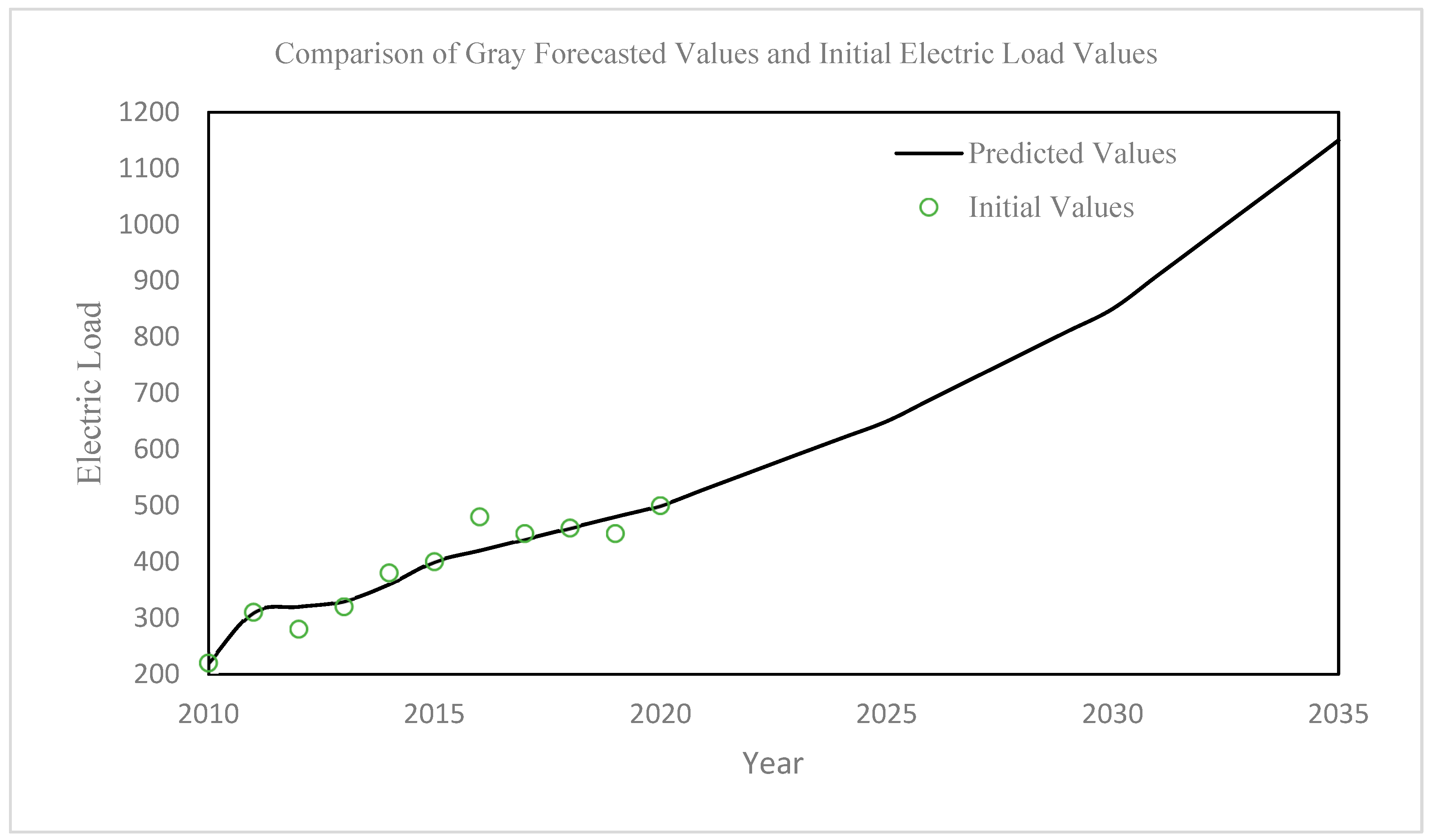
4.2. Optimized Gray Model Long-Term Forecasting

In this section, an optimized gray forecasting model was employed to predict the long-term saturated load in Rudong County for the year 2035. Figure 1 illustrates a comparative analysis between the gray model’s forecast and initial values. The optimized gray model forecasts a saturated load of 1135.67 MW by 2035, significantly lower by approximately 22.49% compared to 1465.37 MW predicted by the spatial load density method. This variance highlights the criticality of selecting appropriate parameters, such as simultaneity rates and load density, in forecasting models. Saturation load, influenced by factors such as GDP, population, land use, and regional economic planning, typically follows an “S” curve, indicating initial growth followed by a plateau phase. The gray forecasting model’s accuracy and universality in load prediction are validated by the literature on GM gray forecasting applications, justifying the retention of the 1135.67 MW forecast in this study.

4.3. VAE-CCNN Long-Term Forecasting

In the development of the neural network model, particularly the Variational Autoencoder and Deep Causal Convolutional Neural Network (VAE-CCNN) hybrid, the selection of input features was guided by a comprehensive analysis of factors influencing load forecasting in large-scale power systems. Recognizing the multifaceted nature of power load patterns, the approach was to incorporate a blend of historical data, temporal variables, and contextual features to enhance the model’s predictive accuracy.

The primary set of input features comprises historical load data, which form the backbone of the forecasting model. These data encompass previous load patterns, capturing the intrinsic temporal fluctuations in power usage. Advanced data processing techniques were employed to ensure the integrity and relevance of the historical data, recognizing their critical role in training the model to recognize and predict future load patterns [34].

Temporal features, including the time of day, the day of the week, and seasonality, were also incorporated. These features are crucial in capturing regular cyclic patterns in electricity usage, such as increased demand during peak hours or seasonal variations. The inclusion of these temporal variables enables the model to account for predictable fluctuations in load demand, enhancing its forecasting precision.

Additionally, contextual features such as weather conditions, economic indicators, and special events, which were identified through literature review and preliminary data analysis as significant influencers of electricity demand, were integrated. Weather conditions, for instance, affect heating and cooling loads, while economic indicators and special events can lead to atypical consumption patterns. By including these contextual variables, the model is equipped to understand and predict load changes in response to external factors.

The selection process for these input features was iterative, involving initial identification based on existing research and domain knowledge, followed by empirical testing. Feature importance analysis methods, such as sensitivity analysis and dimensionality reduction techniques, were employed to refine the feature set, ensuring that only the most impactful parameters were included in the final model.

In summary, the choice of input features for the VAE-CCNN model was a meticulous process, grounded in both theoretical understanding and empirical validation. This careful selection ensures that the model is fed with relevant and influential data, enabling it to generate accurate and reliable load forecasts.

The process and efficacy of employing the VAE-CCNN model for power load forecasting have been outlined above. Model training and parameter tuning, crucial to deep learning forecasting, directly impact prediction accuracy. These processes are detailed below.

• Model Training

Prior to training, the data are divided into training and validation sets. Data from 2010–2017 are used for training, while 2010–2020 data validate the model’s performance. The VAE-CCNN model initializes network weights, with training focused on minimizing mean squared error loss. Predicted values are generated through forward propagation, with error calculated against actual values, followed by backpropagation for weight updates.

• Parameter Tuning

Learning rate: Initially set at 0.01, adjusted to prevent oscillation during training or slow convergence.

Batch size: Set at eight to optimize training speed, considering data volume.

Activation function: ReLU in hidden layers to alleviate gradient vanishing and expedite training.

Optimizer: Adam, for its adaptive learning rate adjustment.

Regularization: L2 to prevent overfitting.

Early stopping: Training halts if there is no significant decrease in validation loss after 10 epochs.

Post-training and tuning, the model’s performance is evaluated using the validation set. This model, now adept at accurately predicting power load, offers valuable insights for future decision-making. A comparison of actual and predicted values is shown in Figure 2.

The comparison between the actual values and the predicted errors is presented in

Table 8. VAE-CCNN-predicted values and actual values comparison table.

Year	Actual Values	Predicted Values	Error
2010	234.90	296.79	26.35%
2011	325.90	307.07	5.78%
2012	278.10	315.51	13.45%
2013	333.50	321.78	3.51%
2014	381.30	351.23	7.89%
2015	396.10	382.41	3.46%
2016	476.70	394.38	17.27%
2017	433.00	404.17	6.66%
2018	447.30	414.35	7.37%
2019	444.60	410.15	7.75%
2020	514.00	518.12	0.80%

.

As indicated in the table, the VAE-CCNN model shows an average error of 9.12% compared to actual values. Its performance is particularly noteworthy in the years 2018, 2019, and 2020, with an end-of-year prediction error in 2020 of just 0.8%. Using the previously mentioned formula, the single regression prediction evaluation function is 1.61, indicating effective forecasting [29]. Based on trends in GDP total, population, policy factors, and industrial proportion, a data table for the years 2021–2035 has been constructed, shown in

Table 9. VAE-CCNN 2021–2035 year forecast table.

Year	GDP Total	Total Population (in 10,000 s)	Policy Factors	Total Societal Maximum Load (MW)
2021	648.36	73.28	0.53	746.72
2022	684.23	72.89	0.51	769.88
2023	720.09	72.50	0.49	795.27
2024	755.93	72.11	0.47	822.41
2025	791.75	71.72	0.46	850.77
2026	827.55	71.33	0.44	879.77
2027	863.34	70.95	0.42	908.87
2028	899.10	70.56	0.41	937.62
2029	934.85	70.18	0.39	965.61
2030	970.59	69.81	0.38	992.53
2031	1006.30	69.43	0.36	1018.18
2032	1042.00	69.06	0.35	1042.43
2033	1077.68	68.68	0.34	1065.25
2034	1113.34	68.32	0.32	1086.68
2035	1148.99	67.95	0.31	1106.82

.

As shown in Table 9, in the VAE-CCNN prediction, the electric power load of Rudong County is expected to reach 1018.18 MW in 2031 and 1106.82 MW in 2035. This represents an 8.71% growth rate within the five years following the carbon peak, but the average annual growth rate is only 1.74%, which is significantly lower than the 5.7% annual growth rate during the Thirteenth Five-Year Plan period. This demonstrates the feasibility of achieving the carbon peak by 2030.

4.4. Medium- and Long-Term Forecast Analysis of Electric Power Load in Rudong County

The VAE-CCNN model, with its advanced predictive capabilities, has demonstrated a significant improvement in forecasting accuracy over traditional methods. For instance, the spatial load density method predicted Rudong County’s electric power load at 1465.37 MW, whereas the optimized VAE-CCNN model forecasted a more refined value of 1106.82 MW. This disparity underscores the enhanced precision of the model, which leverages deep learning techniques to account for non-linearities and complex patterns in the load data that traditional models often overlook.

The spatial load density method relies heavily on load index values, which can introduce a degree of imprecision due to their generalized nature. In contrast, the VAE-CCNN model employs a data-driven approach, processing raw data through a complex neural network to extract nuanced patterns and trends. This methodological shift from reliance on predetermined indices to a more granular, data-centric analysis is a key factor in the increased accuracy of the forecasts.

Considering the limitations of the available data, the OWA operator method was utilized to mitigate the adverse effects of data variability. This approach allowed for the maintenance of the integrity of the forecasts despite data constraints, further highlighting the robustness of the model in dealing with real-world challenges in load forecasting.

The forecasts show a decelerating growth trend in electric power load, aligning with China’s national carbon peak targets. For instance, the projected growth rate decreases to 1.85% from 2034 to 2035, reflecting a conscious shift toward sustainable energy consumption patterns. This aspect of the forecast is particularly relevant, as it provides insights into how energy demand might evolve in the context of national carbon reduction goals.

Traditional forecasting methods, predicting an electric power load as high as 1700 MW for 2035, risk leading to resource misallocation and inefficient grid planning. The proposed approach, which forecasts a significantly lower load of 1210.88 MW, suggests more realistic resource utilization. This is crucial for avoiding scenarios such as premature deployment of high-specification transformers, which could lead to increased costs due to aging-related inefficiencies.

In summary, the study offers a nuanced, data-driven approach to load forecasting that balances accuracy with practical considerations such as national energy goals and resource optimization. By integrating advanced machine learning techniques with a deep understanding of the underlying dynamics of power load, the VAE-CCNN model provides a more realistic and actionable forecast compared to traditional methods. This contribution is particularly significant in the context of sustainable energy planning and the pursuit of carbon neutrality goals.

5. Conclusions

In this study, the integration of the Variational Autoencoder (VAE) with a deep Causal Convolutional Neural Network (Causal CNN) has been pioneered, presenting a significant leap forward in electric power system forecasting. This novel combination has demonstrated superior prediction accuracy, particularly in recent forecasts, where it maintains error control within an impressive 1%. This level of precision marks a notable advancement over traditional methods such as spatial load density and gray forecasting models, which often show considerable deviations due to their dependency on single load indices.

The robustness of the VAE-Causal CNN model has been consistently proven through multiple validations and tests, highlighting its stability and reliability. However, it is crucial to acknowledge that this model’s performance is highly sensitive to data quality. The accuracy, completeness, and integrity of the input data play a decisive role in its practical applications. In response to this, the study has integrated a comprehensive set of factors—including economic, demographic, natural, and random elements—to provide a more holistic and reliable approach to electric power load forecasting. This multidimensional strategy not only ensures the model’s adaptability across various regions and conditions but also underscores its potential for widespread application.

One of the key contributions of this research is the innovative integration of three forecasting methods, particularly through the precise application of the OWA differential operator. This multi-model fusion approach not only enhances the accuracy and robustness of the forecasts but also showcases its unique advantages in the realm of electric power forecasting.

The findings have profound implications for large-scale electric power systems. The models developed in this study offer substantial improvements in terms of accuracy, robustness, and adaptability, thereby providing critical support for grid planning and operational practices. Beyond their immediate application, these models lay a solid theoretical foundation for the future planning and development of electric power systems. It is anticipated that the application of this model in diverse environments and across a broader range will significantly contribute to the stable and efficient operation of power systems.

In conclusion, this study breaks new ground by merging various advanced forecasting technologies to create an innovative and efficient medium- and long-term electric power load forecasting model for systems of 1000 MW scale and above. This model adeptly addresses the evolving load demands of the grid, adheres to stringent stability and reliability criteria, and is poised to make a substantial impact on the strategic planning and operational efficiency of power grids, both theoretically and practically.

Limitations: Despite significant achievements in electric power load forecasting, there are still some limitations. Firstly, the model’s sensitivity to input data noise and variability makes data preprocessing particularly important, adding complexity to practical applications. Secondly, the current model is primarily trained and validated based on data from Rudong County, and its broader generalizability requires further exploration. Additionally, despite using a multi-model fusion strategy, there are other forecasting techniques not considered that might further improve the accuracy of predictions.

Future Work: Considering the above limitations, future research directions could include the following:

• Data Preprocessing and Enhancement: Developing more advanced data cleaning and enhancement techniques to improve model robustness and reduce noise interference in predictions.
• Model Generalization: Applying the model to more regions and power systems, testing its performance in different environments, and further adjusting the model structure for broader adaptability.
• Model Expansion: Exploring and integrating more advanced forecasting techniques to further optimize the multi-model fusion strategy and enhance prediction accuracy and robustness.
• Application Scenario Expansion: Beyond load forecasting, considering the potential applications of the model in other areas of the power system, such as supply reliability and grid optimization.
• Real-time Prediction and Feedback System: Establishing a real-time electric power load forecasting and feedback system, not only predicting future power loads but also making real-time adjustments based on the deviation between actual load and forecasted values, improving the timeliness and accuracy of predictions.

Overall, future work should focus more on the practical application of the model, enhancing robustness, and expanding its use in a broader range of scenarios, providing stronger technical support for the continuous development and optimization of the power system.

References

1. Katsatos, A.L.; Moustris, K.P. Application of Artificial Neuron Networks as energy consumption forecasting tool in the building of Regulatory Authority of Energy, Athens, Greece. Energy Procedia 2019, 157, 851–861. [Google Scholar] [CrossRef]
2. Gao, Y.; Liu, X.; Li, X.; Gu, L.; Cui, J.; Yang, X. A prediction approach on energy consumption for public buildings using mind evolutionary algorithm and bp neural network. In Proceedings of the 2018 IEEE 7th Data Driven Control and Learning Systems Conference (DDCLS), Enshi, China, 25–27 May 2018; IEEE: Piscataway, NJ, USA, 2018; pp. 385–389. [Google Scholar]
3. Barzola-Monteses, J.; Espinoza-Andaluz, M.; Mite-León, M.; Flores-Morán, M. Energy consumption of a building by using long short-term memory network: A forecasting study. In Proceedings of the 2020 39th International Conference of the Chilean Computer Science Society (SCCC), Coquimbo, Chile, 16–20 November 2020; IEEE: Piscataway, NJ, USA, 2020; pp. 1–6. [Google Scholar]
4. Shu, X.; Bao, T.; Li, Y.; Gong, J.; Zhang, K. VAE-TALSTM: A Temporal Attention and Variational Autoencoder-Based Long Short-Term Memory Framework for Dam Displacement Prediction. Eng. Comput. 2021, 38, 3497–3512. [Google Scholar] [CrossRef]
5. Jlidi, M.; Hamidi, F.; Barambones, O.; Abbassi, R.; Jerbi, H.; Aoun, M.; Karami-Mollaee, A. An Artificial Neural Network for Solar Energy Prediction and Control Using Jaya-SMC. Electronics 2023, 12, 592. [Google Scholar] [CrossRef]
6. Chan, S.; Oktavianti, I.; Puspita, V. A deep learning CNN and AI-tuned SVM for electricity consumption forecasting: Multivariate time series data. In Proceedings of the 2019 IEEE 10th Annual Information Technology, Electronics and Mobile Communication Conference (IEMCON), Vancouver, BC, Canada, 17–19 October 2019; IEEE: Piscataway, NJ, USA, 2019; pp. 488–494. [Google Scholar]
7. Shikulskaya, O.; Urumbaeva, O.; Shalaev, T. Concept of Intelligent Energy Grid Control Based on Upgraded Neural Network. In Proceedings of the 2020 International Conference on Electrotechnical Complexes and Systems (ICOECS), Ufa, Russia, 27–30 October 2020; IEEE: Piscataway, NJ, USA, 2020; pp. 1–5. [Google Scholar]
8. Krishnan, M.; Jung, Y.M.; Yun, S. Prediction of energy demand in smart grid using hybrid approach. In Proceedings of the 2020 Fourth International Conference on Computing Methodologies and Communication (ICCMC), Erode, India, 11–13 March 2020; IEEE: Piscataway, NJ, USA, 2020; pp. 294–298. [Google Scholar]
9. Rosato, A.; Araneo, R.; Andreotti, A.; Panella, M. 2-D convolutional deep neural network for multivariate energy time series prediction. In Proceedings of the 2019 IEEE International Conference on Environment and Electrical Engineering and 2019 IEEE Industrial and Commercial Power Systems Europe (EEEIC/I&CPS Europe), Genova, Italy, 11–14 June 2019; IEEE: Piscataway, NJ, USA, 2019; pp. 1–4. [Google Scholar]
10. Rosato, A.; Succetti, F.; Araneo, R.; Andreotti, A.; Mitolo, M.; Panella, M. A Combined Deep Learning Approach for Time Series Prediction in Energy Environments. In Proceedings of the 2020 IEEE/IAS 56th Industrial and Commercial Power Systems Technical Conference (I&CPS), Las Vegas, NV, USA, 29 June–28 July 2020; IEEE: Piscataway, NJ, USA, 2020; pp. 1–5. [Google Scholar]
11. Qi, X.; Zheng, X.; Chen, Q. A short term load forecasting of integrated energy system based on CNN-LSTM. E3S Web Conf. 2020, 185, 01032. [Google Scholar] [CrossRef]
12. Pramono, S.H.; Rohmatillah, M.; Maulana, E.; Hasanah, R.N.; Hario, F. Deep Learning-Based Short-Term Load Forecasting for Supporting Demand Response Program in Hybrid Energy System. Energies 2019, 12, 3359. [Google Scholar] [CrossRef]
13. Kim, T.Y.; Cho, S.B. Particle swarm optimization-based CNN-LSTM networks for forecasting energy consumption. In Proceedings of the 2019 IEEE Congress on Evolutionary Computation (CEC), Wellington, New Zealand, 10–13 June 2019; IEEE: Piscataway, NJ, USA, 2019; pp. 1510–1516. [Google Scholar]
14. Gu, J.; Wang, Z.; Kuen, J.; Ma, L.; Shahroudy, A.; Shuai, B.; Liu, T.; Wang, X.; Wang, G.; Cai, J.; et al. Recent advances in convolutional neural networks. Pattern Recognit. 2018, 77, 354–377. [Google Scholar] [CrossRef]
15. Hochreiter, S.; Schmidhuber, J. Long short-term memory. Neural Comput. 1997, 9, 1735–1780. [Google Scholar] [CrossRef] [PubMed]
16. Bai, S.; Kolter, J.Z.; Koltun, V. An empirical evaluation of generic convolutional and recurrent networks for se-quence modeling. arXiv 2018, arXiv:1803.01271. [Google Scholar]
17. Kingma, D.P.; Welling, M. Auto-Encoding Variational Bayes. In Proceedings of the ICLR, Banff, Canada, 14–16 April 2014. [Google Scholar]
18. Vanting, N.B.; Ma, Z.; Jørgensen, B.N. A scoping review of deep neural networks for electric load forecasting. Energy Inform. 2021, 4, 49. [Google Scholar] [CrossRef]
19. Nti, I.K.; Teimeh, M.; Nyarko-Boateng, O.; Adekoya, A.F. Electricity load forecasting: A systematic review. J. Electr. Syst. Inf. Technol. 2020, 7, 13. [Google Scholar] [CrossRef]
20. Wang, H.; Lei, Z.; Zhang, X.; Zhou, B.; Peng, J. A review of deep learning for renewable energy forecasting. Energy Convers. Manag. 2019, 198, 111799. [Google Scholar] [CrossRef]
21. Aguiar-Pérez, J.M.; Pérez-Juárez, M.Á. An Insight of Deep Learning Based Demand Forecasting in Smart Grids. Sensors 2023, 23, 1467. [Google Scholar] [CrossRef] [PubMed]
22. Sharma, K.; Dwivedi, Y.K.; Metri, B. Incorporating causality in energy consumption forecasting using deep neural networks. Ann. Oper. Res. 2022, 69, 1–36. [Google Scholar] [CrossRef] [PubMed]
23. GB/T50293-2014; Code for Urban Electric Power Planning. Chinese Standard: Beijing, China, 2014.
24. Trivedi, R.; Khadem, S. Implementation of artificial intelligence techniques in microgrid control environment: Current progress and future scopes. Energy AI 2022, 8, 100147. [Google Scholar] [CrossRef]
25. Fekri, M.N.; Grolinger, K.; Mir, S. Distributed load forecasting using smart meter data: Federated learning with Recurrent Neural Networks. Int. J. Electr. Power Energy Syst. 2022, 137, 107669. [Google Scholar] [CrossRef]
26. Luo, X.J.; Oyedele, L.O. Forecasting building energy consumption: Adaptive long-short term memory neural networks driven by genetic algorithm. Adv. Eng. Inform. 2021, 50, 101357. [Google Scholar] [CrossRef]
27. Li, G.; Jung, J.J. Deep learning for anomaly detection in multivariate time series: Approaches, applications, and challenges. Inf. Fusion 2023, 91, 93–102. [Google Scholar] [CrossRef]
28. Khodayar, M.; Regan, J. Deep Neural Networks in Power Systems: A Review. Energies 2023, 16, 4773. [Google Scholar] [CrossRef]
29. O’Shaughnessy, M.; Canal, G.; Connor, M.; Rozell, C.; Davenport, M. Generative causal explanations of black-box classifiers. Adv. Neural Inf. Process. Syst. 2020, 33, 5453–5467. [Google Scholar]
30. Massaoudi, M.; Abu-Rub, H.; Refaat, S.S.; Chihi, I.; Oueslati, F.S. Deep learning in smart grid technology: A review of recent advancements and future prospects. IEEE Access 2021, 9, 54558–54578. [Google Scholar] [CrossRef]
31. Huang, J.; Guan, L.; Su, Y.; Yao, H.; Guo, M.; Zhong, Z. Recurrent graph convolutional network-based multi-task transient stability assessment framework in power system. IEEE Access 2020, 8, 93283–93296. [Google Scholar] [CrossRef]
32. Chen, Y.; Kang, Y.; Chen, Y.; Wang, Z. Probabilistic forecasting with temporal convolutional neural network. Neurocomputing 2020, 399, 491–501. [Google Scholar] [CrossRef]
33. Liu, J.; Yang, G.; Li, X.; Hao, S.; Guan, Y.; Li, Y. A deep generative model based on CNN-CVAE for wind turbine condition monitoring. Meas. Sci. Technol. 2022, 34, 035902. [Google Scholar] [CrossRef]
34. GT/T50441-2016; Residential Building Energy Consumption Standard. Chinese Standard: Beijing, China, 2016.
Figure 1. Comparison of gray forecasted values and initial electric load values.
Sustainability 16 01710 g001
Figure 2. Comparison of gray forecasted values and initial electric load values. VAE-CCNN-predicted values and actual values comparison.
Sustainability 16 01710 g002