The Economic Effects of Stormwater Best Management Practices (BMPs) on Housing Sale Prices in Washington, D.C.

Abstract

This study aims to investigate the economic effects of stormwater best management practices (BMPs) on housing sale prices in Washington, D.C., BMPs play a significant role in mitigating multiple threats, such as water pollution, soil erosion, and property damage. While studies on the economic value of BMPs were limited, literature addresses that housing sale prices can be affected by nearby stormwater BMPs. This study addresses the following research questions: Do stormwater BMPs positively impact housing sale prices? How do proximity and number of structural BMPs affect the housing sale prices? We used the hedonic pricing method by applying multiple linear regression models to determine whether a set of independent variables significantly improved the models. Our primary findings indicate that BMPs have positive, negative, or no effects on housing sale prices. The proximity of BMPs inside of parks increased housing sale prices in all buffers. In contrast, the proximity of BMPs outside of parks and impervious roads decreased housing sale prices in all buffers. Percent tree canopy coverage negatively linked to a 50 m buffer and had no relationship with other buffers on housing sale prices. This study implies that BMPs impact housing prices and can be improved by landscape architects, policymakers, and stakeholders.

1. Introduction

Stormwater runoff causes multiple threats to the environment as land development progresses and precipitation event intensity increases. During heavy rains, faster runoff changes the water volume and increases the velocity, which conveys pollutants, degrades ecosystems, and damages property [1,2]. As awareness of the management of stormwater sources increases, structural stormwater best management practices (BMPs), such as trees, detention basins, and retention basins, play a significant role in mitigating runoff issues, integrating environmental concerns, and improving the sustainable growth of development [3,4].

The concept of stormwater BMPs, as a part of green infrastructure, has been addressed within the last two decades [5]. After the United States Environmental Protection Agency (EPA) adopted the National Pollutant Discharge Elimination System (NPDES) permit program in the early 1990s, regulations of water runoff were established from municipalities, construction activities, and industrial sources in the United States [6]. The regulations for stormwater management in Washington, D.C., have been in place since 1988. The primary goal of the regulation was to reduce stormwater pollution by using BMPs, which have the capability of channeling, retaining, and absorbing stormwater [7].

While numerous studies have focused on specific physical and biological effects of stormwater BMPs [8], studies of the economic impact of stormwater BMPs on housing sale prices were limited. This research addresses the following two questions: Do stormwater BMPs positively impact housing sale prices? How do proximity and number of structural BMPs affect the housing sale prices?

2. Literature Review

Previous research indicates that stormwater BMPs provide positive, negative, or no economic effects on housing prices. These studies primarily use the hedonic pricing method. This method enables deconstruction of the price of an asset into the asset’s various component parts: environmental, structural, locational, and neighborhood attributes by using the Arc geographical information system (GIS) analysis tool to measure percent (e.g., tree canopy coverage), proximity/distance buffer, and count of BMPs.

Studies show that trees contribute to housing sale prices [9,10,11,12,13]. Housing sale prices increase as tree canopy coverage increases between a 100 m and 150 m buffer [9]. The percentage/number of street trees within a 100 ft (30.5 m) positively impacted housing prices, and street trees increased housing sale prices by an average of $8870 [10]. Netusil et al. [11] found that increased tree canopy coverage increased property benefits from 7.21% to 8.21% ($149–$528). Li [12] also found that the value of properties near tree planting locations (e.g., within a 10 m buffer) increased by 1.2% in housing sale prices. A 10% increase in trees per street (per 100 m) added a 0.03% to 0.05% premium to property prices [13]. This author also found that trees within 10–50 m of the property added a 0.02–0.05% premium to property prices. Meanwhile, housing sale prices decreased as tree canopy coverage increased within a 25 m buffer [9]. In addition, the west side of Portland decreased property sale prices as tree canopy coverage increased [11].

Studies show that impervious surfaces contribute to housing sale prices [14,15]. The mean impervious surface area in a 500 m neighborhood surrounding each property was negatively related to housing sale prices [14]. The viewshed of the area of impervious surfaces was negatively related to housing sale prices [15]. In contrast, the mean area of impervious surfaces within 500 m of the home was positively related to housing sale prices [15].

Previous studies showed that BMPs inside of parks positively influence housing prices compared to BMPs outside of parks. Distance to BMPs inside parks was linked to housing prices [16]. The authors found that residential property values decreased by $ 164.82 as the 10 m distance was far from the BMPs inside parks. Meanwhile, there was no evidence of the effect of distance to BMPs inside parks on housing property value beyond 274 m (900 ft). In addition, distance to BMPs outside of parks had no significant effect on housing property value [16].

In summary, previous literature has shown that stormwater BMPs provide valuable benefits, negative effects, or no effects on housing sale prices. Numerous studies addressed that BMPs support a sustainable environment, enhance economic feasibility by offsetting the high cost of grey infrastructure [5], and develop aesthetic values when the design, maintenance, and specific concerns of BMPs are well managed [17,18,19].

The primary purpose of this study is to assess the contributions of economic effects of stormwater BMPs on housing sale prices in Washington, D.C., USA. The hedonic price model was applied to analyze the statistical impact of environmental attributes while controlling for a set of housing structural, locational and neighborhood, and ward variables.

3. Materials and Methods

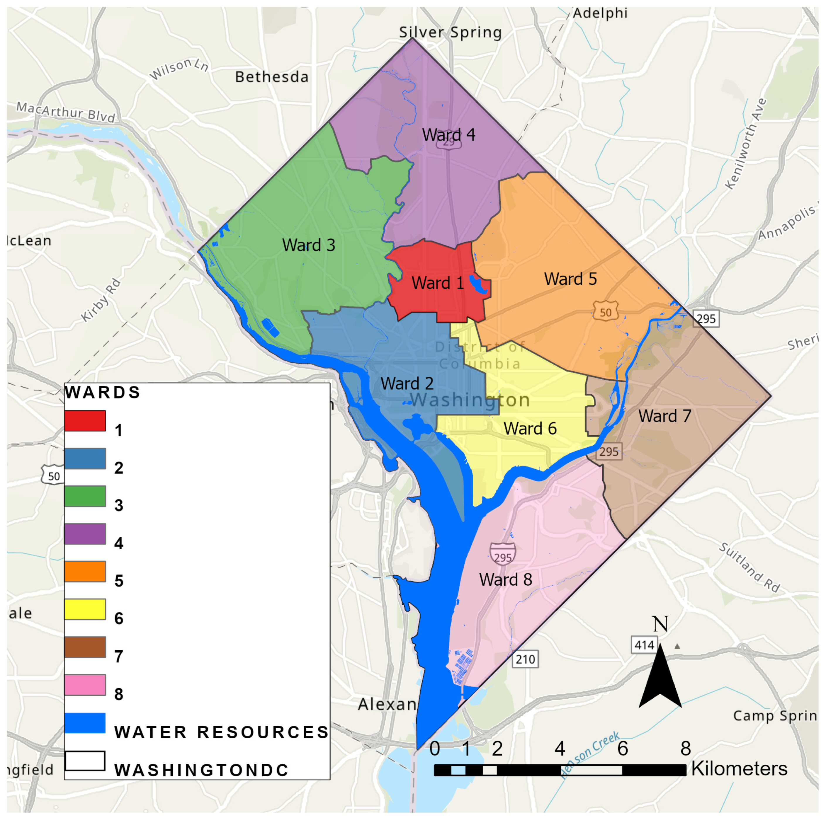
3.1. Study Area

The geographic setting for this study is Washington, District of Columbia (D.C.), which is in the mid-Atlantic region of the eastern United States. The District has an approximate area of 177 km² and is composed of three individual water bodies with eight individual wards (Figure 1). Three major water resources (e.g., Anacostia River, Rock Creek, and Potomac River) flow into the District from the outside jurisdiction. While the Potomac River is on the south side of the District, the Anacostia River is on the east side of the district, and Rock Creek is on the north side of the District. Water in the District is operated by two primary wastewater collection systems: “combined” and “separate” sewers [20]. The population of D.C. was 671,803 in 2022 with a population of 46.2% White, 45.0% Black, 4.7% Asian, and 11.7% Hispanic/Latino [21]. The District’s estimated median household income was $101,722 in 2022 in U.S. dollars [21]. The average tree canopy coverage was 37% in 2021 and the District is planning to increase tree canopy coverage up to 40% by 2032, which was linked to an annual planting target of 8600 trees/year [22].

3.2. Data and Measurement

The hedonic pricing method was developed after the listwise deletion to assess the impact of stormwater BMPs on housing sale prices for each analysis. Data were processed and analyzed using Microsoft^® Excel 2401, Statistical Package for the Social Sciences (SPSS^®) 26.0, and ArcGIS Pro 3.2.0. The dependent variable for the multiple regression model was the logged housing sale prices. The housing sale prices data were collected January 2017–December 2020 from both computer-assisted mass appraisal (CAMA)—residential data—and common ownership lots data from the District’s open access dataset: Department of Energy and Environment (DOEE) (

Table 1. Variables, measurement, and unit (n = 4537).

Variables	Measurement	Unit
Housing sale price (logged)	Single-family Housing sale price = logged (price)	US dollar ($)
Environmental variables
Proximity
House to parks with BMPs	Euclidean distance from housing parcel to parks parcel with BMPs	(m)
House to parks with no BMPs	Euclidean distance from housing parcel to parks parcel without BMPs	(m)
House to BMPs inside of parks	Euclidean distance from housing parcel to BMPs points inside of the parks	(m)
House to BMPs outside of parks	Euclidean distance from housing parcel to BMPs points outside of the parks	(m)
Count
25 m BMPs	Number of BMPs within 25 m buffer from housing parcel	(Count)
50 m BMPs	Number of BMPs within 50 m buffer from housing parcel	(Count)
75 m BMPs	Number of BMPs within 75 m buffer from housing parcel	(Count)
100 m BMPs	Number of BMPs within 100 m buffer from housing parcel	(Count)
Landcover
25 m tree coverage	Tree coverage within 25 m donut buffer from housing parcel	(%)
50 m tree coverage	Tree coverage within 50 m donut buffer from housing parcel	(%)
75 m tree coverage	Tree coverage within 75 m donut buffer from housing parcel	(%)
100 m tree coverage	Tree coverage within 100 m donut buffer from housing parcel	(%)
25 m impervious surfaces	Impervious surfaces within 25 m donut buffer from housing parcel	(%)
50 m impervious surfaces	Impervious surfaces within 50 m donut buffer from housing parcel	(%)
75 m impervious surfaces	Impervious surfaces within 75 m donut buffer from housing parcel	(%)
100 m impervious surfaces	Impervious surfaces within 100 m donut buffer from housing parcel	(%)
25 m impervious roads	Impervious roads within 25 m donut buffer from housing parcel	(%)
50 m impervious roads	Impervious roads within 50 m donut buffer from housing parcel	(%)
75 m impervious roads	Impervious roads within 75 m donut buffer from housing parcel	(%)
100 m impervious roads	Impervious roads within 100 m donut buffer from housing parcel	(%)
Structural variables
Lot size	Parcel size	Logged (ft²)
Bathroom	Number of total bathrooms	(Count)
Air conditioner	Air conditioner = 1; others = 0	(0/1)
Bedroom	Number of bedrooms	Sqrt (Count)
Building size	Gross building area in square feet	(ft²)
Age of building	Building age	(year)
Remodeled age	Remodeled age of housing structure	(year)
Structural grade rating	=1 (lowest) to 12 (highest)
Structural condition rating	=1 (lowest) to 6 (highest)
Fireplaces	Fireplaces = 1; others = 0	(0/1)
Locational and neighborhood variables
Population density	Population/Total area in square meters at census tract
Crime	Number of reported crimes/total population at census tract
Unemployment	Unemployment rate in census tract	(%)
Income	Median Income in census tract	US dollar ($)
Vacancy	Vacancy rate in census tract	(%)
Poverty	Poverty rate in census tract	(%)
Age	Median age of residence	(year)
Moved 2017 or later	Number of years living (tenure) 2017 or later in census tract	(%)
Moved 2015–2016	Number of years living (tenure) 2015–2016 in census tract	(%)
Moved 2010–2014	Number of years living (tenure) 2010–2014 in census tract	(%)
Moved 2000–2009	Number of years living (tenure) 2010–2009 in census tract	(%)
Moved 1990–1999	Number of years living (tenure) 1990–1999 in census tract	(%)
Moved 1989–earlier (Reference group)	=0 in all moved population categories
Public schools	Euclidean distance from housing parcel polygon to public schools point	(m)
Grocery stores	Euclidean distance from housing parcel polygon to grocery stores point	(m)
Religious centers	Euclidean distance from housing parcel polygon to worships point	(m)
Shopping centers	Euclidean distance from housing parcel polygon to shopping centers point	(m)
Wards
High-income ward	Median income ($111,064–$128,670) = 1, otherwise = 0	(0/1)
Medium-income ward	Median income ($94,810–$102,882) = 1, otherwise = 0	(0/1)
Low-income ward (Reference group)	Median income ($35,245–$71,782) = 1, otherwise = 0	(0/1)

). CAMA data provided housing sale prices and housing structural information, such as lot size, number of bathrooms, and housing sizes. We combined both CAMA and common ownership lots data since common ownership lots data provided geographical locations of each housing parcel and housing sale prices, which allowed us to analyze it using ArcGIS Pro. The initial total sample was n = 24,084. After sorting the data by including only single-family properties—detached, row, and semi-detached houses—we removed outliers in the range of $16,323–$31,537,500 and below $16,000. Six duplicates of housing addresses were found after checking three real estate websites including Zillow, Trulia, and Redfin to match the correct structural information (e.g., number of bedrooms and number of bathrooms). Finally, 4537 total addresses remained after applying a listwise deletion approach.

The measurements and units of environmental, structural, locational and neighborhood, and ward variables are given in Table 1. Best management practices data were obtained between 2016 and 2020 from DOEE. The BMPs data include three types of BMPs: bioretention, rainwater harvesting, and tree planting and preservation. The data provided information such as geographical locations, BMPs type, installation date, surface area of BMPs, and volume of BMPs.

Land cover data were obtained from the Chesapeake Conservancy (2022) in partnership with the U.S. Geological Survey (USGS). The meter resolution data were referred to as Land Use/Land Cover Data Project 2017/2018, which attributed to 54 detailed classes and 18 general classes. High-resolution satellite imagery with different minimum mapping units for each class was represented: water, wetlands, tree canopy, shrubland, low vegetation, barren, structures, impervious surfaces, impervious roads, tree canopy over structures, tree canopy over impervious surfaces, and tree canopy over impervious roads. The following indicators of land cover data were used in this study: tree canopy coverage, impervious surfaces, and impervious roads by drawing a nine-square-meter minimum mapping unit. The preparation of the land cover data was generated by calculating the percent tree canopy coverage, percent impervious surfaces, and percent impervious roads. The buffer analysis in ArcGIS Pro was used to calculate 25 m, 50 m, 75 m, and 100 m from the housing property parcel.

Parks data were obtained from DOEE. Parks in the data set consisted of three different data: national parks, parks and recreation areas, and community gardens. To measure the proximity of parks and locations of BMPs associated with parks, data estimated the proximity of houses to parks with BMPs, parks with no BMPs, BMPs inside of parks, and BMPs outside of parks variables. Beginning with the BMPs and parks data, this study used Euclidean distance in meters from each property sold to the nearest variable to calculate using the Near Analysis function in ArcGIS Pro. This process repeated for the distance from each property to the nearest parks with BMPs, parks with no BMPs, BMPs inside of parks, and BMPs outside of parks. To determine the count of BMPs, the number of BMPs within every 25 m buffer from housing property parcels was calculated by using buffer analysis and the spatial join tool in ArcGIS Pro. This process was repeated in 25 m, 50 m, 75 m, and 100 m. In the buffer analysis, we excluded the area of the housing parcel and included the overlap buffer area (e.g., 50 m buffer included 25 m buffer area).

To determine the effect of land cover on housing sale prices, the buffer analysis was used with ArcGIS Pro. The percentage of tree canopy coverage, impervious surfaces, impervious roads, tree canopy over structure, tree canopy over impervious surfaces, and tree canopy over impervious roads were calculated for every 25 m buffer from the housing property parcel polygon. This process was repeated in 25 m, 50 m, 75 m, and 100 m. The limit of the buffer from housing parcels was 100 m because the area beyond the 100 m buffer was outside of Washington, D.C.

The structural characteristics of the selected single-family houses such as lot size, building age, and number of bathrooms and bedrooms were derived from DOEE and specified in statistical models to control for capitalization effects.

The locational and neighborhood characteristics of the selected single-family houses such as population density, median income, and distance to public schools and shopping centers were derived from DOEE and specified in statistical models.

The District has eight wards. Three ward groups were categorized based on the median income range. The range of the high-income ward group was from $111,064 to $128,670, the range of the medium-income ward group was from $94,810 to $102,882, and the range of the low-income ward group was from $35,245 to $71,782. Based on the range, wards 1, 2, 3, and 6 belong to the high-income ward group. Wards 4 and 5 belong to the medium-income ward group, and wards 7 and 8 belong to the low-income ward group.

3.3. Analytical Procedures: Hedonic Pricing Method

Residential properties are composed of heterogeneous characteristics, which makes the estimation of housing values challenging. The hedonic pricing method is one of the tools that has been used and analyzed enormously in the housing market [23]. This method estimates the contribution of individual characteristics, such as housing structure, and locational or environmental amenities using statistical approaches [23,24]. Established by Lancaster’s theory [25], the hedonic pricing method addresses physical and other heterogeneous features (e.g., geographical location, occupancy), which can be often unobserved by homeowners [26]. These factors might be considerable for homeowners when they purchase their homes. In this sense, housing sale prices are determined by a group of several factors. They consist of environmental, structural, and locational and neighborhood attributes, which is the functional form of the empirical model that can be expressed as follows:

$$\mathrm{HP}=f(x_1, x_2, x_3, x_4, \cdots , x_i),$$

(1)

where HP is the housing sale prices of individual properties, and $x_1, x_2, x_3, x_4\dots , x_{\mathrm{i}}$ indicate heterogeneous dimensions of housing characteristics. The heterogeneous features can be divided into several groups. The model can be expressed as follows:

$$\mathrm{HP}=\alpha +{\beta }_{1}S+{\beta }_{2}L+{\beta }_{3}E+\mathrm{\epsilon },$$

(2)

where HP is an (n × 1) vector of housing prices; S is an (n × i) matrix of housing structure attributes; L is an (n × j) matrix of locational attributes; E is an (n × k) matrix of neighborhood environmental attributes. α is constant, and ${\beta }_1$, ${\beta }_2$, ${\beta }_3$ are the estimated parameter vectors, and ε is an (n × 1) vector of error terms, which is normally distributed with a zero mean and constant variance.

A multiple-parametric hedonic function was used. The estimation method of the multiple linear regression model was employed, which can take the form of the following [27]:

$$y={\beta }_0+{\beta }_1{x}_1+{\beta }_2{x}_2+{\beta }_3{x}_3+\dots +{\beta }_v{x}_v+\mathrm{\epsilon },$$

(3)

where y is the dependent variable, and $x_1$, $x_2, x_3\dots , x_v$ are the independent variables that explain the value of $x$ or on which y depends. The betas (${\beta }_0, {{\beta }_1, \beta }_2,\dots , {\beta }_v)$ are unknown parameters to be estimated from the equation and ε is error terms. This parameter is assumed to be normally distributed with a mean of zero and a constant variance ${\sigma }^2$ [28].

The estimator of the multiple linear regression model is the ordinary least squares (OLS) estimation, which is an unbiased estimator by minimizing the sum of squared regression residuals to estimate housing sale prices [29]. The assumption of OLS is that error terms are independently distributed, samples are independent of each other, and the dependent variables and independent variables are exogenous.

This study used the model with variables: (1) environmental, (2) structural, (3) locational and neighborhood, and (4) wards. These four sets of variables were put into the model as the following formula:

$$\ln P_i=\alpha +{\beta }_1{E}_i+{\beta }_2{S}_j +{\beta }_3{L}_k+{\beta }_4{W}_m+{\mathrm{\epsilon }}_i,$$

(4)

where ln$P_i$ is the log of the housing sale prices $i$; $E_i$ is a vector of environmental variables, including proximity of house to parks with BMPs, house to parks with no BMPs, house to BMPs inside of parks, house to BMPs outside of parks, count of BMPs with 25 m, 50 m, 75 m, 100 m, tree canopy coverage with 25 m, 50 m, 75 m, 100 m, impervious surface with 25 m, 50 m, 75 m, 100 m, and impervious roads with 25 m, 50 m, 75 m, 100 m; $S_j$ is a vector of structural variables, including lot size, total number of bathrooms, number of bedrooms, building size, building age, remodeled age, structural grading rating, structural condition rating, fire places, years of living (tenure) at the census tract, and air conditioner as a dummy; $L_k$ is a vector of locational and structural variables, including population density, crime rate, unemployment rate, median income, vacancy, poverty rate at the census tract, median age of residence, and distance to public schools, grocery stores, religious centers, and shopping centers; $W_m$ is a vector of wards including high, median, and low median income as dummy variables.

The coefficients to be estimated are ${\beta }_1$, ${\beta }_2$, ${\beta }_3$, and ${\beta }_4$, and ε is an error term. Therefore, housing sale prices are transformed into logs, which are interpreted as the price percentage changes resulting from one additional unit of the independent variable approximately. The R-square ($R^2$) of the model increases as additional independent variables are introduced in the model. The increment of $R^2$ prior sets was not affected by the subsequent groups of explanatory variables [24], which can be shown as follows:

$${R^2}_{\mathrm{Y}·\mathrm{E}\mathrm{S}\mathrm{L}\mathrm{W}}={R^2}_{\mathrm{Y}·\mathrm{E}}+{R^2}_{\mathrm{Y}·(\mathrm{E}·\mathrm{S})}+{R^2}_{\mathrm{Y}·(\mathrm{E}·\mathrm{S}·\mathrm{L})}+{R^2}_{\mathrm{Y}·(\mathrm{E}·\mathrm{S}·\mathrm{L}·\mathrm{W})},$$

(5)

where ${R^2}_{\mathrm{Y}·\mathrm{E}\mathrm{S}\mathrm{L}\mathrm{W}}$ is the coefficient of determination of the full model; ${R^2}_{\mathrm{Y}·\mathrm{E}}$ is the coefficient of determination of the model only including a set of environmental variables; ${R^2}_{\mathrm{Y}·(\mathrm{E}·\mathrm{S})}$ is the increment of the coefficient of determination of the model including environmental variables and structural variables; ${R^2}_{\mathrm{Y}·(\mathrm{E}·\mathrm{S}·\mathrm{L})}$ is the increment of the coefficient of determination of the model including environmental variables, structural variables, and locational and neighborhood variables. ${R^2}_{\mathrm{Y}·(\mathrm{E}·\mathrm{S}·\mathrm{L}·\mathrm{W})}$ is the increment of the coefficient of determination of the model including environmental variables, structural variables, locational and neighborhood variables, and ward variables.

4. Results

4.1. Descriptive Statistics

We weighted data by ward groups to correct the under-representation issue of the low-income ward so our data can accurately represent the population before analysis (

Table 2. Summary statistics for wards before data weighted.

Variables	Mean	Median	Standard Deviation	Min	Max
Wards (dummy)
High-income ward	0.59	0.00	0.49	0.00	1.00
Medium-income ward	0.34	0.00	0.47	0.00	1.00
Low-income ward (Reference group)	0.07	0.00	0.24	0.00	1.00

).

Table 3. Summary statistics for environmental, structural, locational and neighborhood, and ward variables after data weighted (n = 4537).

Variables	Mean	Median	Standard Deviation	Min	Max
Housing sale price (2017–2020 US$)	1,105,715.386	909,384.59	881,163.58	77,000	17,750,000
Housing sale price (logged)	5.965	5.959	0.249	4.9	7.2
Environmental variables
Proximity
House to parks with BMPs	623.13	551.94	421.02	0.00	2409.87
House to parks with no BMPs	179.24	155.31	121.86	0.00	671.40
House to BMPs inside of parks	847.29	760.87	495.43	45.22	2639.97
House to BMPs outside of parks	84.20	66.38	74.31	0.00	619.98
Count
25 m BMPs (sqrt)	0.24	0.00	0.58	0.00	4.00
50 m BMPs (sqrt)	0.60	0.00	0.87	0.00	4.58
75 m BMPs (sqrt)	0.97	1.00	1.02	0.00	4.90
100 m BMPs (sqrt)	1.35	1.41	1.15	0.00	5.57
Landcover
25 m tree coverage (%)	38.96	37.62	17.80	0.00	96.35
50 m tree coverage (%)	37.82	36.40	16.95	0.44	96.67
75 m tree coverage (%)	37.25	35.94	15.72	2.55	92.69
100 m tree coverage (%)	37.13	35.34	15.55	2.20	90.93
25 m impervious surfaces (%)	9.26	7.77	6.83	0.00	54.93
50 m impervious surfaces (%)	9.49	8.29	6.59	0.00	53.01
75 m impervious surfaces (%)	10.12	9.01	6.49	0.08	46.83
100 m impervious surfaces (%)	10.46	9.55	6.36	0.14	38.38
25 m impervious roads (%)	17.45	17.00	7.95	0.00	53.76
50 m impervious roads (%)	16.59	16.37	6.92	0.00	43.72
75 m impervious roads (%)	16.47	16.55	5.66	0.76	38.15
100 m impervious roads (%)	16.26	16.42	5.28	1.34	35.72
Structural variables
Lot size (lg_ft²)	8.08	8.16	0.74	5.54	10.65
Bathroom (count)	3.04	3.00	1.15	0.5	12.5
Air conditioner (dummy)	0.93	1.00	0.24	0.00	1.00
Bedroom (Sqrt_count)	3.75	4.00	1.24	1.00	47.00
Building size (ft²)	1937.17	1696.00	928.70	528	14,126
Age of building (year)	91.94	92.00	23.82	6.00	240.00
Remodeled age (year)	11.04	7.00	12.81	0.00	109.00
Structural grade rating	1.18	1.16	0.22	0.75	2.90
Structural condition rating	1.08	1.07	0.05	0.79	1.23
Fireplaces (dummy)	0.11	0.00	0.17	0.00	1.00
Locational and neighborhood variables
Population density (%)	0.51	0.38	0.35	0.09	2.47
Crime (%)	15.24	12.00	9.94	2.00	54.00
Unemployment (%)	6.32	4.90	4.77	0.20	31.6
Income (median)	123,293.79	121,176.00	55,755.94	14,413	250,001
Vacancy (%)	1.52	0.00	2.50	0.00	13.10
Poverty (%)	7.38	3.30	9.45	0.00	63.50
Age	37.59	38.40	6.01	20.00	47.30
Moved 2017 or later (%)	10.12	9.58	5.38	0.00	32.05
Moved 2015–2016 (%)	25.70	24.80	8.84	3.61	59.02
Moved 2010–2014 (%)	14.88	14.71	5.04	2.06	41.77
Moved 2000–2009 (%)	16.83	16.05	6.15	3.80	35.18
Moved 1990–1999 (%)	10.02	9.01	5.50	0.00	22.44
Moved 1989–earlier (%) (Reference group)	13.70	11.96	8.78	0.47	45.45
Distance to public schools (m)	494.86	428.44	296.97	23.74	1884.71
Distance to grocery stores (m)	835.84	684.28	561.97	34.16	3373.67
Distance to religious centers (m)	270.63	195.77	253.38	0.00	1946.87
Distance to shopping centers (m)	1383.99	1059.76	1129.95	43.97	5609.40
Distance to Capitol (m)	5980.53	5938.30	2633.09	526.70	11,982.89
Wards (dummy)
High-income ward	0.51	1.00	0.49	0.00	1.00
Medium-income ward	0.25	0.00	0.43	0.00	1.00
Low-income ward (Reference group)	0.23	0.00	0.42	0.00	1.00

Note. Moved 1989–earlier (%) is reference group; low-income ward is reference group.

provides descriptive statistics including the housing sale prices, environmental variables, structural variables, locational and neighborhood variables, and ward variables after data is weighted. We used a listwise deletion approach to exclude any missing cases to compare the results among different buffer distances.

4.1.1. Environmental Variables

The mean proximity of houses to parks with BMPs was 623.13 m, while the mean proximity of houses to parks with no BMPs was 179.24 m. This indicated that the mean proximity of houses to parks with BMPs was further than the mean proximity of houses to parks with no BMP. In other words, people could easily access the parks regardless of BMPs. The mean proximity of houses to BMPs inside the parks was 847.29 m, while the mean proximity of houses to BMPs outside of parks was 84.20 m. This indicated that the mean proximity of houses to BMPs inside of parks was further than the mean proximity of houses to BMPs outside of parks, and BMPs themselves were located near housing property. The mean count of BMPs was increased from 0.24 to 1.35 as every 25 m buffer increased from the property. The mean percentage of tree canopy coverage consistently decreased from 38.96% to 37.13% as every 25 m buffer increased from the property. The mean percentage of impervious surfaces consistently increased from 9.26% to 10.46% as every 25 m buffer increased from the property. The mean percentage of impervious roads consistently decreased from 17.45% to 16.26% as every 25 m buffer increased from the property.

4.1.2. Structural Variables

The mean number of bathrooms was 3.04, and the number of bedrooms was 3.75. The mean age of the building was 91.94 years. The oldest age of the building was 240 years, and the youngest age of the building was 6 years.

4.1.3. Locational and Neighborhood Variables

The mean crime rate at the census tract was 15.24%. The mean age of the population at the census tract was 37.59. The mean distance to the U.S. Capitol from the property was 5980.53 m, which was the farthest distance among other variables. The mean distance to religious centers was 270.63 m, which was the shortest distance among other variables.

4.1.4. Ward Variables

Unweighted data showed that the mean high-income wards group was 0.59, the mean medium-income wards group was 0.34, and the mean low-income ward group was 0.07 (Table 2). After the data were weighted, the mean high-income ward group became 0.51, the mean medium-income ward group became 0.25, and the mean low-income ward group became 0.23 (Table 3). Our weighted data represented the proportion of each ward group better than the unweighted data.

4.2. Hedonic Price Model

This study uses the hedonic price model to determine the contributing effect of several independent variables on the dependent variable to estimate whether a set of independent variables significantly improved the hedonic price model.

Table 4. A summary of regression analysis, including environmental, structural, locational and neighborhood, and ward variables.

Variables	25 m	50 m	75 m	100 m
Variable intercept	4.150 ***	4.177 ***	4.188 ***	4.196 ***
Environmental variables
Proximity
House to parks with BMPs	−0.005	−0.006	−0.004	−0.003
House to parks no BMPs	0.007	0.007	0.007	0.008
House to BMPs inside of parks	−0.041 ***	−0.040 ***	−0.041 ***	−0.042 ***
House to BMPs outside of parks	0.016 **	0.017 **	0.018 **	0.017 *
Buffer
Count of BMPs	0.001	0.000	−0.001	−0.002
Landcover
% tree canopy coverage	−0.012	−0.026 **	−0.010	−0.010
% impervious surfaces	0.013	0.001	−0.009	−0.014
% impervious roads	−0.020 **	−0.029 ***	−0.016 *	−0.016 *
Structural variables
Lot size	0.149 ***	0.146 ***	0.141 ***	0.139 ***
Number of bathrooms	0.125 ***	0.125 ***	0.126 ***	0.126 ***
Air conditioner (dummy)	0.012 *	0.012 **	0.011 *	0.011 *
Number of bedrooms	0.053 ***	0.053 ***	0.053 ***	0.052 ***
Building size	0.177 ***	0.178 ***	0.178 ***	0.178 ***
Building age	0.043 ***	0.043 ***	0.043 ***	0.043 ***
Remodeled age	−0.049 ***	−0.049 ***	−0.049 ***	−0.049 ***
Structural grade rating	0.203 ***	0.201 ***	0.201 ***	0.201 ***
Structural condition rating	0.142 ***	0.142 ***	0.142 ***	0.142 ***
Number of fireplaces	0.029 ***	0.030 ***	0.031 ***	0.030 ***
Locational and neighborhood variables
Population density	0.038 ***	0.038 ***	0.043 ***	0.044 ***
% of crime rate	−0.028 ***	−0.028 ***	−0.025 ***	−0.024 ***
Unemployment rate	−0.049 ***	−0.049 ***	−0.047 ***	−0.046 ***
Median income	0.135 ***	0.135 ***	0.134 ***	0.134 ***
Vacancy rate	−0.007	−0.006	−0.006	−0.005
Poverty rate	−0.016	−0.016	−0.016	−0.016
Age	0.031***	0.031 ***	0.029 ***	0.028 ***
Moved 2017 or later	0.032 ***	0.032 ***	0.031 ***	0.030 ***
Moved 2015–2016	0.029 ***	0.030 ***	0.028 ***	0.028 ***
Moved 2010–2014	−0.008	−0.007	−0.008	−0.008
Moved 2000–2009	−0.042 ***	−0.041 ***	−0.044 ***	−0.044 ***
Moved 1990–1999	0.009	−0.009	0.008	0.007
Moved 1989–earlier (Reference group)
Distance to public schools	−0.019 **	−0.018 **	−0.017 **	−0.016 **
Distance to grocery stores	−0.025 ***	−0.025 ***	−0.026 ***	−0.026 ***
Distance to religious centers	0.042 ***	0.041 ***	0.039 ***	0.038 ***
Distance to shopping centers	−0.045 ***	−0.045 ***	−0.044 ***	−0.044 ***
Distance to Capitol	−0.018	−0.018	−0.021 *	−0.021 *
Wards (dummy)
High-income ward	0.462 ***	0.462 ***	0.464 ***	0.465 ***
Medium-income ward	0.242 ***	0.242 ***	0.244 ***	0.246 ***
Low-income ward (Reference group)
$R^2$	0.900	0.900	0.899	0.899

Note. Dependent variable: logged housing sale prices 2017–2020; standardized β is reported in all variables. * p ≤ 0.05, ** p < 0.01, *** p < 0.001.

includes environmental, structural, locational and neighborhood, and ward variables. The summary of the multiple regression includes coefficient, significance, and R-squared in all buffers (25 m, 50 m, 75 m, and 100 m).

We also examined the variance inflation factors (VIFs) to detect multicollinearity while running multiple regression models. None of the independent variables had VIF values greater than 10. All 51 independent variables were kept, and the variance of the dependent variable was well explained by the independent variables.

The multiple regression model includes environmental, structural, locational and neighborhood, and ward variables (Table 4). The proximity of houses to BMPs inside of parks is significantly predicted on housing sale prices in all buffers: 25 m (β = −0.041, p < 0.001); 50 m (β = −0.040, p < 0.001); 75 m (β = −0.041, p < 0.001); and 100 m (β = −0.042, p < 0.001). The coefficient for the proximity of houses to BMPs inside of parks is all negative, which is associated with an increase in housing sale prices as the proximity of BMPs inside of parks decreased. While controlling for other covariates, a 1 unit decrease in the proximity of houses to BMPs inside of parks is associated with a −0.041 unit increase in 25 m; −0.040 in 50 m; −0.041 in 75 m; and −0.042 in 100 m. The coefficient for the proximity of houses to BMPs inside of parks within 25–50 m increased the most from −0.041 to −0.040 (d = 0.001). The coefficient for proximity of houses to BMPs inside of parks within 25–100 m decreased the most from −0.041 to −0.042 (d = −0.001) and 75–100 m from −0.041 to −0.042 (d = −0.001).

The proximity of houses to BMPs outside of parks is significantly predicted on housing sale prices in all buffers: 25 m (β = 0.016, p < 0.01); 50 m (β = 0.017, p < 0.01); 75 m (β = 0.018, p < 0.01); and 100 m (β = 0.017, p ≤ 0.05). The coefficient for the proximity of houses to BMPs outside of parks is all positive, which is associated with an increase in housing sale prices as the proximity of BMPs outside of parks increased. While controlling for other covariates, a 1 unit increase in the proximity of houses to BMPs inside of parks is associated with a 0.016 unit increase in 25 m; 0.017 in 50 m; 0.018 in 75 m; and 0.017 in 100 m. The coefficient for the proximity of houses to BMPs outside of parks within 25–75 m increased the most from 0.016 to 0.018 (d = 0.002). The coefficient for the proximity of houses to BMPs outside of parks within 75–100 m decreased the most from 0.018 to 0.017 (d = −0.001).

Percent tree canopy coverage is significantly predicted on housing sale prices in 50 m (β = −0.026, p < 0.01), and the coefficient is negative. This indicates that housing sale prices decrease as there is an increase in tree canopy coverage within a 50 m buffer from the property.

Percent impervious roads are significantly predicted on housing sale prices in 25 m (β = −0.020, p < 0.01); 50 m (β = −0.029, p < 0.001); 75 m (β = −0.016, p ≤ 0.05); 100 m (β = −0.016, p ≤ 0.05), and the coefficient is all negative. This indicates that housing sale prices decrease as the percentage of impervious roads increases from 25 m to 75 m then the coefficient for 100 m is kept.

All the structural characteristics of the selected single-family houses such as lot size, building age, and number of bathrooms and bedrooms are statistically predicted on housing sale prices in all models. Increases in lot size and number of bedrooms are associated with higher housing sale prices. In contrast, increases in the remodeling age of buildings are associated with lower housing sale prices.

All the locational and neighborhood variables, except vacancy rate, poverty rate, percent move 2010–2014, percent move 1990–1999, and near distance to the U.S. Capitol (25 m and 50 m), are significantly predicted on housing sale prices. Increases in population density and median income are associated with higher housing sale prices. In contrast, increases in crime rate and unemployment rate are associated with lower housing sale prices.

Both high-income and medium-income ward groups are significantly predicted on housing sale prices. Increases in both high-income and medium-income ward groups are associated with higher housing sale prices.

Overall, the R-squared values for 25 m ($R^2=$ 0.900), 50 m ($R^2=$ 0.900), 75 m ($R^2=$ 0.899), and 100 m ($R^2=$ 0.899) are given. Table 4 shows high performance; independent variables well-explain 89–90% of the variances in single-family housing sale prices, respectively.

5. Discussion

Our findings of this study provide insights into how stormwater BMPs economically affect housing sale prices in Washington, D.C. The results of our multiple regression analysis indicate that the proximity of houses to BMPs outside of the parks may be considered as an unattractive option for property owners (Table 4). This unattractiveness might be due to aging or poor maintenance of BMPs. For instance, the aging of BMPs might deteriorate surrounding areas and prevent the natural bioremediation process [30]. Poor maintenance might cause concerns, such as accumulating sediment at inlet and outlet structures or increasing diseases through mosquitoes [31,32], which generate an unpleasant environment and alter ecosystem services [33]. Thus, people may not be willing to install BMPs adjacent to their properties, which negatively affects housing sale prices [33,34].

In contrast, the proximity of BMPs inside parks was an indicator of purchasing homes for property owners, according to the regression analysis (Table 4). Studies showed that the adjacency of the parks was a critical factor that increased the property’s value [35], or the presence of green space positively affected the housing value [36]. Moreover, public parks with a regular maintenance schedule could manage stormwater BMPs, recreational amenities, and other ecosystems, which can generate value for housing prices.

A majority of previous studies have addressed that tree canopy coverage increases housing sale prices [9,10,11,12,13]. Various buffers are used to estimate the effect of tree canopy coverage (e.g., 10 m, 30.5 m, and 10–50 m). Our results show the opposite results from the previous findings, which indicate that the percent tree canopy coverage decreases housing sale prices in the 50 m buffer in the regression model. This might be due to the maintenance of trees. Trees also entail maintenance costs, such as watering, pruning, and fixing root damage, which is not an attractive investment for property owners. This factor might lead to a lack of tree canopy coverage, which indicates that the average tree canopy coverage is 37.0% (2021), below the District’s 40% tree canopy goal [22]. In addition, residents might not prefer planting trees on their properties due to safety concerns (e.g., falling trees, broken branches).

Percent of impervious roads decreases housing sale prices in all buffers in the regression model. Properties close to impervious roads might be associated with more traffic, pollution, noise, and other possible dis-amenities that decrease housing sale prices [14].

The findings suggest several considerations for further study. Increasing the number of BMPs inside parks could increase housing sale prices. Considering the diverse welfare effects of BMPs, social benefits might be expected by improving the surrounding landscapes, recreational opportunities, and accessibility, which might encourage stakeholders and municipalities to understand the value of BMPs.

Sustainable maintenance of BMPs should be developed since those concerns have negative economic effects associated with environmental, infrastructure, and regulatory problems [37,38]. Conservation of trees with proper maintenance (e.g., monitoring) is as important as tree planting. Because diverse species have different growth rates, treating their characteristics could help achieve the District’s goal and improve the ecosystem. These associations bear further study and might prevent environmental gentrification, which is linked to the monetary value of stormwater BMPs. Well-maintained conditions of the environment offer better performance and aesthetic values, which increase the public’s perception of BMPs. Considerations of systematic design of BMPs with proper maintenance are highly recommended for long-term value. Well-maintained BMPs would function properly, which decreases the maintenance cost and generates long-term benefits for properties. In addition, the proper regulatory plan should be initiated and performed for BMPs, whether their locations are inside or outside of parks. Supportive regulations, such as zoning restrictions or subsidy options regarding planting trees, could also encourage residents to consider having trees on their properties.

Moreover, the housing market fluctuates over time and is affected by other external factors, such as structural, locational, and neighborhood attributes. Using panel data helps better understand housing market trends by analyzing pre- and post-construction of BMPs while controlling for the years’ effects. In addition, the economic effects of BMPs might be accurate by controlling other variables, such as the view of BMPs and education level. Such external factors were ruled out in this research since there were data limitations, as our study includes only single-family houses that may feature homogeneous characteristics.

The analytical framework of spatial statistics might need to be addressed. Geographic distribution of some attributes addresses potential spatial dependence or spatial autocorrelation, which is one of the limitations of the traditional hedonic pricing method [29,39]. Further research should be considered on spatial econometrics (e.g., spatial lag or spatial error models) to compare the models, or artificial intelligence models, such as neural networks, might be performed as an alternative method to test a broader range of variation in the output than the hedonic regression method [40].

6. Conclusions

This research aimed to investigate the economic effects of stormwater BMPs on housing sale prices. This study addresses specific research questions: Do stormwater BMPs positively impact housing sale prices? How do the proximity and number of structural BMPs affect the housing sale prices?

Our robust findings conclude that the economic effects of stormwater BMPs have positive, negative, or no effects on housing sale prices. Proximity of BMPs outside of parks decreases the housing sale prices in all buffers in our regression model. Meanwhile, the proximity of BMPs inside parks increases the housing sale prices in all buffers. The percentage of tree canopy coverage decreases the housing sale prices in the 50 m buffer. The percentage of impervious roads decreased the housing sale prices in all buffers.

Therefore, these results provide incentives for property owners to consider how BMPs could benefit their communities, even though concerns remain. For this reason, sustainable strategies with sufficient regulations (e.g., management guidelines and landscaping code) can enhance green performance. Financial support (e.g., rebate program) should be improved by policymakers, landscape architects, planners, and community stakeholders for the long-term value of serving environmental, social, and economic benefits of BMPs.

References

1. Braden, J.B.; Johnston, D.M. Downstream economic benefits from storm-water management. J. Water Resour. Plan. Manag. 2004, 130, 498–505. [Google Scholar] [CrossRef]
2. National Research Council. Urban Stormwater Management in the United States; National Academies Press: Washington, DC, USA, 2009. [Google Scholar]
3. Arnold, C.L., Jr.; Gibbons, C.J. Impervious surface coverage: The emergence of a key environmental indicator. J. Am. Plann. Assoc. 1996, 62, 243–258. [Google Scholar] [CrossRef]
4. Schueler, T.R. Stormwater Pond and Wetland Options for Stormwater Quality Control; EPA Seminar Publication: Chicago, IL, USA, 1993. [Google Scholar]
5. Breuste, J.; Artmann, M.; Li, J.; Xie, M. Special issue on green infrastructure for urban sustainability. J. Urban Plan. Dev. 2015, 141, A2015001. [Google Scholar] [CrossRef]
6. Fletcher, T.D.; Shuster, W.; Hunt, W.F.; Ashley, R.; Butler, D.; Arthur, S.; Trowsdale, S.; Barraud, S.; Semadeni-Davies, A.; Bertrand-Krajewski, J.L.; et al. SUDS, LID, BMPs, WSUD and more–The evolution and application of terminology surrounding urban drainage. Urban Water J. 2015, 12, 525–542. [Google Scholar] [CrossRef]
7. The Department of Energy and the Environment. Consolidated Total Maximum Dily Load (TMDL) Implementation Plan Report. Available online: https://dcstormwaterplan.org/wp-content/uploads/TMDL_IP_09132022_Final.pdf (accessed on 12 December 2023).
8. Steinnes, D.N. Measuring the economic value of water quality: The case of lakeshore land. Ann. Reg. Sci. 1992, 26, 171–176. [Google Scholar] [CrossRef]
9. Boslett, A.J. Hedonic Analyses of Urban Green Spaces and Urban Tree Cover in Syracuse, NY. Master’s Thesis, State University of New York College of Environmental Science and Forestry, Syracuse, NY, USA, 2011. [Google Scholar]
10. Donovan, G.H.; Butry, D.T. Trees in the city: Valuing street trees in Portland, Oregon. Landsc. Urban Plan. 2010, 94, 77–83. [Google Scholar] [CrossRef]
11. Netusil, N.R.; Chattopadhyay, S.; Kovacs, K.F. Estimating the demand for tree canopy: A second-stage hedonic price analysis in Portland, Oregon. Land Econ. 2010, 86, 281–293. [Google Scholar] [CrossRef]
12. Li, L. The Effect of Urban Tree Planting on Residential Property Values and Gentrification. Doctoral Dissertation, University of Illinois at Urbana-Champaign, Champaign, IL, USA, 2020. [Google Scholar]
13. Overwater, T. Trees under Urban Pressure: A Case Study on Understating the Effect of Public Street Trees on Property Prices in Highly Urban Amsterdam. Master’s Thesis, University of Groningen, Groningen, The Netherlands, 2020. [Google Scholar]
14. Sander, H.; Polasky, S.; Haight, R.G. The value of urban tree cover: A hedonic property price model in Ramsey and Dakota Counties, Minnesota, USA. Ecol. Econ. 2010, 69, 1646–1656. [Google Scholar] [CrossRef]
15. Sander, H.A.; Haight, R.G. Estimating the economic value of cultural ecosystem services in an urbanizing area using hedonic pricing. J. Environ. Manag. 2012, 30, 194–205. [Google Scholar] [CrossRef] [PubMed]
16. Lee, J.S.; Li, M.H. The impact of detention basin design on residential property value: Case studies using GIS in the hedonic price modeling. Landsc. Urban Plan. 2009, 89, 7–16. [Google Scholar] [CrossRef]
17. Ferguson, B.K. Taking advantage of stormwater control basins in urban landscapes. JWSC 1991, 46, 100–103. [Google Scholar]
18. Emmerling-DiNovo, C. Stormwater detention basins and residential locational decisions. JAWRA 1995, 31, 515–521. [Google Scholar] [CrossRef]
19. Hamilton, K.; Hindman, P.; Wegener, K. Water Quality and Multi-Use Improvements to a Storm Runoff Detention Facility/State Dam. In Bridging the Gap: Meeting the World’s Water and Environmental Resources Challenges; ASCE Publishing: Reston, VA, USA, 2001. [Google Scholar]
20. DC Water Is Life. Available online: https://www.dcwater.com/css (accessed on 12 December 2023).
21. United States Census Bureau. Available online: https://www.census.gov/quickfacts/fact/table/DC/PST045222 (accessed on 12 December 2023).
22. District of Columbia Urban Tree Plan. 2021. Available online: https://caseytrees.org/treereportcard2021/ (accessed on 12 December 2023).
23. Kong, F.; Yin, H.; Nakagoshi, N. Using GIS and landscape metrics in the hedonic price modeling of the amenity value of urban green space: A case study in Jinan City, China. Landsc. Urban Plan. 2007, 79, 240–252. [Google Scholar] [CrossRef]
24. Malpezzi, S. Hedonic pricing models: A selective and applied review. In Housing Economics and Public Policy; Wiley-Blackwell: Hoboken, NJ, USA, 2002; pp. 67–89. [Google Scholar]
25. Lancaster, K.J. A new approach to consumer theory. J. Pol. Econ. 1966, 74, 132–157. [Google Scholar] [CrossRef]
26. Sheppard, S. Chapter 41. Hedonic analysis of housing markets. In Handbook of Regional and Urban Economics, 1st ed.; Cheshire, P., Mills, E.S., Eds.; Elsevier: Amsterdam, The Netherlands, 1999; Volume 3, pp. 1595–1635. [Google Scholar]
27. Owusu-Ansah, A. A review of hedonic pricing models in housing research. Int. J. Civ. Eng. 2011, 1, 19. [Google Scholar]
28. Cohen, J.; Cohen, P.; West, S.G.; Aiken, L.S. Applied Multiple Regression/Correlation Analysis for the Behavioral Sciences, 3rd ed.; Routledge: New York, NY, USA, 2002. [Google Scholar]
29. Huang, Z.; Chen, R.; Xu, D.; Zhou, W. Spatial and hedonic analysis of housing prices in Shanghai. Habitat Int. 2017, 67, 69–78. [Google Scholar] [CrossRef]
30. United States Congress. Bioremediation for Marine Oil Spills; Office of Technology Assessment: Washington, DC, USA, 1991. [Google Scholar]
31. Blecken, G.T.; Hunt, I.I.I.W.F.; Al-Rubaei, A.M.; Viklander, M.; Lord, W.G. Stormwater control measure (SCM) maintenance considerations to ensure designed functionality. Urban Water J. 2017, 14, 278–290. [Google Scholar] [CrossRef]
32. Jackson, M.J.; Gow, J.L.; Evelyn, M.J.; Meikleham, N.E.; McMahon, T.S.; Koga, E.; Howay, T.J.; Wang, L.; Yan, E. Culex mosquitoes, West Nile virus, and the application of innovative management in the design and management of stormwater retention ponds in Canada. Water Res. 2009, 44, 103–110. [Google Scholar] [CrossRef]
33. Irwin, N.B.; Klaiber, H.A.; Irwin, E.G. Do stormwater basins generate co-benefits? Evidence from Baltimore County, Maryland. Ecol. Econ. 2017, 141, 202–212. [Google Scholar] [CrossRef]
34. Jauregui, A.; Fan, Q.; Curry, J. House Price Capitalization of Stormwater Retention Basins: Evidence from Fresno-Clovis Metropolitan Area in California. J. Real Estate Finance Econ. 2021, 67, 606–626. [Google Scholar] [CrossRef]
35. Nicholls, S.; Crompton, J.L. The impact of greenways on property values: Evidence from Austin, Texas. J. Leis. Res. 2005, 37, 321–341. [Google Scholar] [CrossRef]
36. Peiser, R.B.; Schwann, G.M. The private value of public open space within subdivisions. J. Archit. Plan. Res. 1993, 1, 91–104. [Google Scholar]
37. Taguchi, V.J.; Weiss, P.T.; Gulliver, J.S.; Klein, M.R.; Hozalski, R.M.; Baker, L.A.; Finlay, J.C.; Keeler, B.L.; Nieber, J.L. It is not easy being green: Recognizing unintended consequences of green stormwater infrastructure. Water 2020, 12, 522. [Google Scholar] [CrossRef]
38. Pantaloni, M.; Marinelli, G.; Santilocchi, R.; Minelli, A.; Neri, D. Sustainable Management Practices for Urban Green Spaces to Support Green Infrastructure: An Italian Case Study. Sustainability 2022, 14, 4243. [Google Scholar] [CrossRef]
39. Des Rosiers, F.; Thériault, M.; Villeneuve, P.Y. Sorting out access and neighbourhood factors in hedonic price modelling. J. PrOP. Investig. Finance 2000, 18, 291–315. [Google Scholar] [CrossRef]
40. Selim, H. Determinants of house prices in Turkey: Hedonic regression versus artificial neural network. Expert Syst. Appl. 2009, 36, 2843–2852. [Google Scholar] [CrossRef]
Figure 1. Study area Washington, D.C., with wards and water resources. Note. Map sources: Esri, HERE, Garmin, FAO, NOAA, USGS, © OpenStreetMap contributors and the GIS User Community.
Sustainability 16 01498 g001