Article

High Spatiotemporal Remote Sensing Images Reveal Spatial Heterogeneity Details of Soil Organic Matter

1
State Key Laboratory of Black Soils Conservation and Utilization, Northeast Institute of Geography and Agroecology, Chinese Academy of Sciences, Changchun 130102, China
2
University of Chinese Academy of Sciences, Beijing 100049, China
3
School of Public Administration and Law, Northeast Agricultural University, Harbin 150030, China
*
Author to whom correspondence should be addressed.
Sustainability 2024, 16(4), 1497; https://doi.org/10.3390/su16041497
Submission received: 2 January 2024 / Revised: 2 February 2024 / Accepted: 7 February 2024 / Published: 9 February 2024

Abstract

:
Soil is the foundation of sustainable agricultural development. Soil organic matter (SOM) is a key indicator for characterizing soil degradation, and remote sensing has been applied in SOM prediction. However, the differences in SOM prediction from different remote sensing data and the ability to combine multi-source and multi-phase remote sensing data for SOM prediction urgently need to be explored. The following research employed Landsat-8, Sentinel-2, and Gaofen-6 satellite data, utilizing a random forest algorithm to establish a SOM prediction model. It aimed to explore the variations in SOM prediction capabilities among these satellites in typical black soil regions. Additionally, the study involved creating multi-phase synthetic images for SOM prediction using Landsat-8 and Sentinel-2 images captured during three years of bare soil periods. Finally, the research examined the ability to combine three satellites to construct high spatiotemporal remote sensing images for SOM prediction. The results showed that (1) using Landsat-8 and Sentinel-2 to extract the principal components of the three-year bare soil period to construct the multi-phase synthetic image for SOM prediction, higher prediction accuracies can be obtained compared with the single-phase images. (2) The highest accuracy can be obtained using multi-phase synthetic images and high spatial resolution images to construct high spatiotemporal remote sensing images and perform SOM prediction (R2 is 0.65, RMSE is 0.67%, MAE is 0.42%). (3) Simultaneously, high spatiotemporal remote sensing images can reach 2 m spatial resolution to reveal the spatial heterogeneity of SOM. The causes of SOM spatial anomalies can be determined after analysis combined with soil degradation information. In subsequent research, SOM prediction should focus more on multi-sensor collaborative prediction.

1. Introduction

Soil plays a crucial role in ensuring the sustainability of agricultural practices. Soil organic matter (SOM) is a crucial component of soil, serving as a key indicator of soil nutrient status [1]. SOM enhances soil fertility through various processes [2,3]. Additionally, SOM is a major sink and source of carbon in the Earth’s largest carbon reservoir, soil carbon [4]. Northeast China is one of the world’s four major black soil regions [5]. This fertile soil plays a vital role in China’s significant food production. However, due to long-term unscientific farming practices, the soil in this region faces a severe risk of nutrient loss. Studies indicate that since the 1980s, 64% of the cultivated soil in Northeast China has experienced a decline in SOM [6]. The rapid and accurate acquisition of SOM information, covering large areas with high spatial resolution, is significant for precise farmland management and macro-level decision-making [7].
Satellite remote sensing technology has become the mainstream method for soil element prediction mapping by overcoming the previous disadvantages of traditional soil elements, e.g., difficulty covering large areas and time-consuming processes [8,9,10]. Current SOM mapping mainly uses satellite remote sensing images during the bare soil period [11]. The bare soil period is when vegetation objects do not cover the surface soil [12]. For the black soil area in Northeast China, April to May every year is the bare soil period [13]. The bare soil period provides a time window for remote sensing monitoring of soil elements. During this period, the cultivated land is not covered by vegetation, straw, and snow; the soil is completely exposed on the land surface. Current SOM mapping based on remote sensing images is mainly based on a single satellite sensor [14]. Ye et al. used Gaofen-6 images to predict soil SOM in Hefei, China, based on random forest (RF), light gradient boosting machine (LightGBM), gradient boosting tree (GBDT), and extreme boosting machine (XGBoost) prediction models [15].
Along with the significant increase in the number of remote sensing satellites, the vast amount of remote sensing data provides new opportunities for earth observation, such as expanding the scope of surface coverage, more intensive observation, diversifying the functions of sensors, and obtaining surface information from more perspectives. From the perspective of data reliability, multi-source remote sensing data can be verified with each other, and at the same time, ensure the continuity of remote sensing data and provide a data basis for multi-scale–multi-source remote sensing data fusion [16].
The vast number of satellites and remote sensing data also brings new challenges, and different satellites have differences in sensor characteristics, data quality, observational specialties, and shortcomings, which need more assessment and validation [17,18,19]. Dong et al. addressed the radiometric calibration problem of the wide field of view (WFV) imaging of Gaofen-1 and Gaofen-6. They used Landsat-8 OLI as a reference sensor to obtain a finer image observation dataset to improve the radiometric calibration accuracy of the Gaofen-6 images [20]. Guo et al. analyzed the consistency of band reflectance between Gaofen-1 and Gaofen-6 for the same type of remote sensing satellites [21]. Li et al. compared the performance of Landsat-8 and Landsat-9 in monitoring and identifying salt pines on the west coast of the U.S., and the results showed that the performance of the two satellites was basically the same [22]. Shi et al. compared Gaofen-6 with Sentinel-2 in monitoring Chlorophyll-a concentration in small water bodies, and the Gaofen-6 imagery showed higher spatial resolution, while Sentinel-2 had a faster temporal response [23]. Xia et al. utilized Landsat-8, Sentinel-2, and Gaofen-2 images to compare the performance of the three satellite sensors for mapping soil pH in the black soil region based on the quantitative random forest (QRF) method [24]. A series of studies have been conducted to analyze the performance of different multispectral satellites. However, these studies focus on remote sensing SOM prediction methods, input data, and other issues, but they focus on a single satellite. Today, when remote sensing data sources are becoming more and more diverse, we need more comprehensive and detailed comparative studies and utilization of various multispectral satellites for SOM prediction.
Gaofen-6 was launched in 2018. The Gaofen-6 satellite has a multispectral high-resolution camera (PMS) with a multispectral spatial resolution of 8 m and a panchromatic spatial resolution of 2 m [25]. Compared with the 30 m and 10 m spatial resolutions of the widely used Landsat and Sentinel satellites, the Gaofen-6 satellite has raised the spatial resolution of Earth observations to a new level. However, as a new generation of remote sensing satellites, Gaofen-6 faces the test of authenticity and has few applications in SOM mapping in black soil areas.
In this study, Landsat-8, Sentinel-2, and Gaofen-6 images were acquired for the bare soil period of 2020, 2021, and 2022 in the typical black soil area of Northeast China, construct a SOM prediction model using the random forest method, with the following specific research objectives. (1) What are the differences in SOM prediction among the three satellites with different spatial resolutions? (2) Can the SOM prediction accuracy be improved using multi-phase bare soil images compared with single-phase images? (3) Attempting to construct high spatiotemporal remote sensing images by combining multi-phase synthetic images and high spatial resolution images in order to improve the SOM prediction accuracy and reveal spatial heterogeneity details of SOM.

2. Materials and Methods
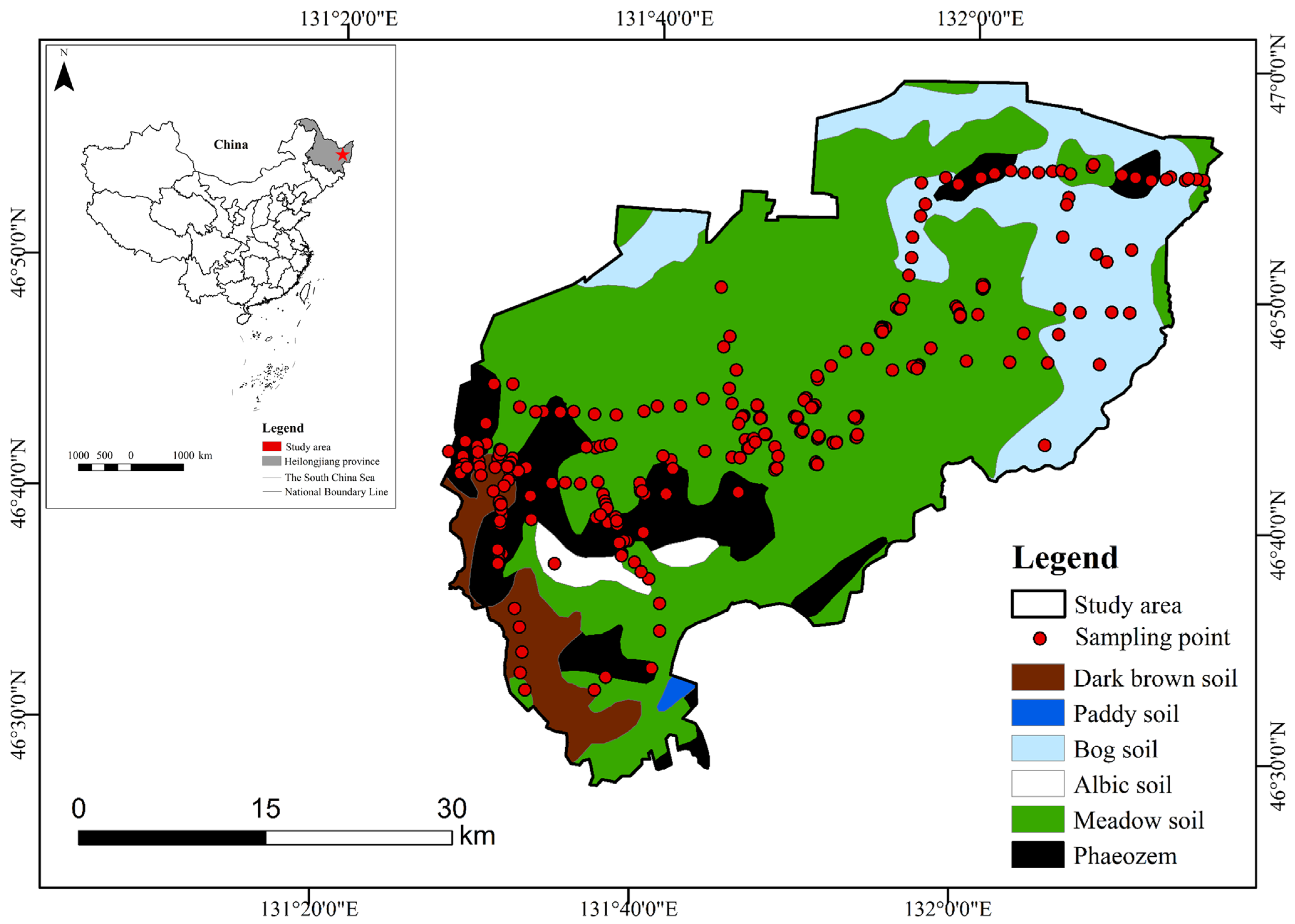
2.1. Study Area

The study area comprised Youyi Farm, Heilongjiang Province, Northeast China. The farm has a total controlled area of 188,813 ha (Figure 1), of which 110,429 ha are cultivated. It has a mid-temperate continental monsoon climate with rainy summers and long, cold winters, an average annual precipitation of 514 mm, and an average frost-free period of 143 days. The western part of the study area has undulating terrain, while the eastern part is flat. There are soil degradation problems, such as water erosion and desertification, in the central and western areas. The main soil types are black soil, meadow soil, swampy soil, dark brown soil, and fertile soil. The main crops that are cultivated are corn, soybean, and rice.

2.2. Soil Sampling and Analysis

The soil samples used in this study were collected in March–April 2021 and early June 2022 due to the more stable retention of SOM in the soil [26]. During this period, the cultivated soils had rested after approximately five months of winter, and soil properties remained stable. Two hundred and seventy-nine soil samples were collected in the study area by considering soil types and topographic features. Portable GNSS loggers located the soil sample collection locations. The distribution of the collection sites is shown in Figure 1. The collected soil samples were air-dried, ground, and sieved to obtain soil particles of less than 2 mm diameter. Then, the SOM content was determined using the external heating–potassium dichromate titration method [27].

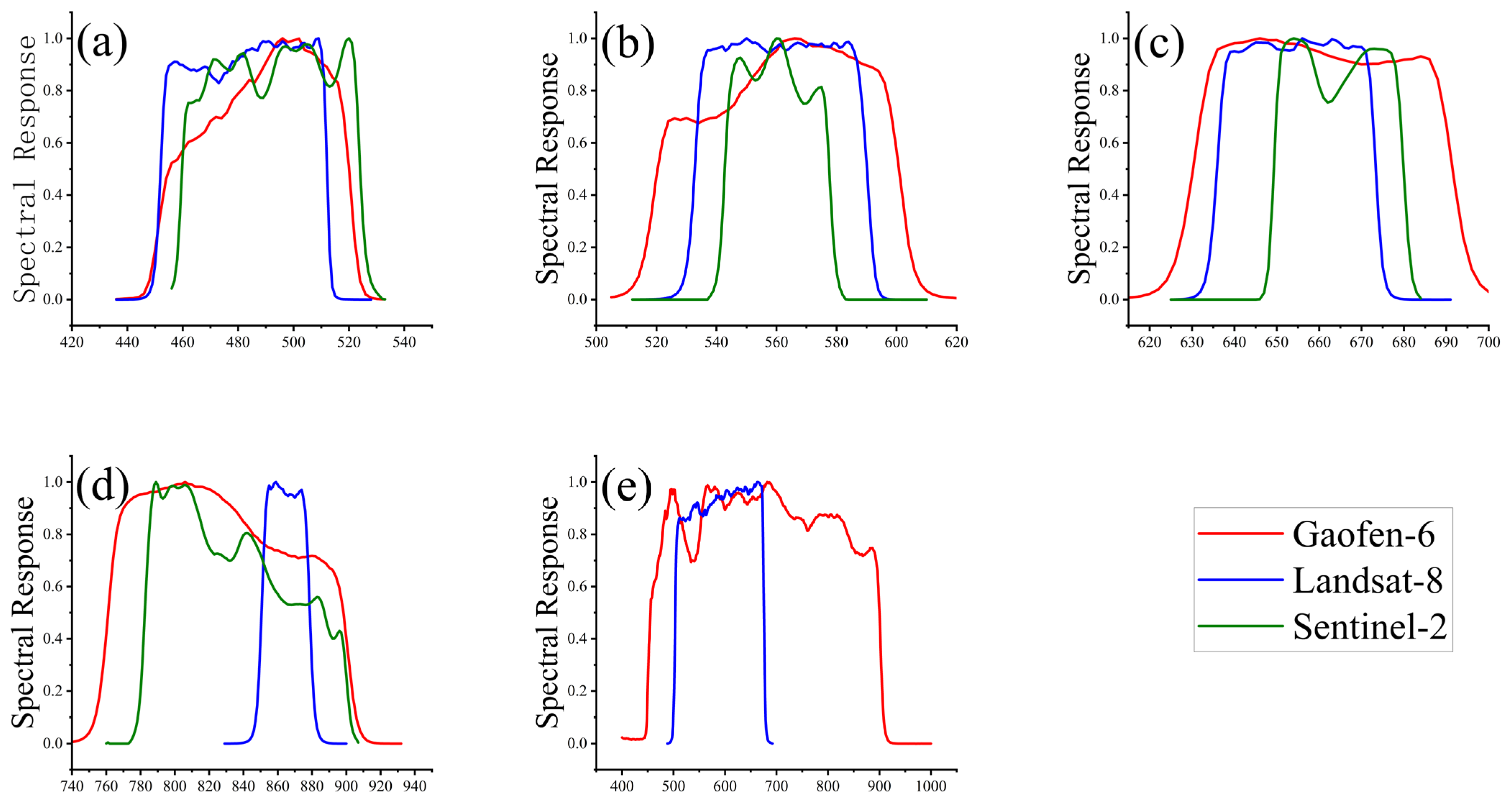
2.3. Remote Sensing Image Acquisition and Preprocessing

2.3.1. Landsat-8/Landsat-9 OLI Image

The USGS provides Landsatd-8 and Landsat-9 surface reflectance products, which correct for the spectral scattering and absorption effects of atmospheric gases, aerosols, and water vapor. This study obtained the Landsat-8/Landsat-9 surface reflectance data of the study area during the three-year bare soil period in 2020, 2021, and 2022 from the Google Earth Engine, with 6 images.

2.3.2. Sentinel-2 MSI Image

The ESA provides Sentinel-2 with two data classes, Level-1C and Level-2A. Level-1C is a geometrically corrected top-of-atmosphere reflectance product, and Level-2A is an atmospherically corrected surface reflectance product based on Level-1C. In this study, Sentinel-2 surface reflectance data were obtained from the Google Earth Engine for three years, 2020, 2021, and 2022, for the bare soil period in the study area, with 13 images.

2.3.3. Gaofen-6 PMS Image

The original Gaofen-6 PMS image must undergo orthorectification, radiometric calibration, and atmospheric correction preprocessing. Then, the preprocessed PMS image and the radiometrically calibrated and orthorectified Gaofen-6 panchromatic band image were fused to obtain a multispectral image with a spatial resolution of 2 m [27]. This study obtained the Gaofen-6 PMS image on 16 April 2020 from the China Earth Observation and Data Center website.
The spectral response function is an essential parameter of remote-sensing satellite sensors [17,28]. Figure 2 shows the spectral response functions of the three sensors, Landsat-8 OLI, Sentinel-2 MSI, and Gaofen-6 PMS, for the five bands of red, green, blue, near-infrared, and panchromatic. Among the five bands, the panchromatic band has the most significant difference, with a difference of 270 nm in the response range between the two bands. Next is the near-infrared band. The response function of Gaofen-6 PMS is closer to Sentinel-2 MSI, and the difference with Landsat-8 OLI is even more significant. The differences between the spectral response ranges of the red, green, and blue bands are subtle. Overall, the Landsat-8 OLI sensor is closer to the ideal square wave spectral response function, while the Gaofen-6 PMS sensor has more significant fluctuations.

2.4. SOM Prediction Model

SOM prediction using remote sensing images is based on the fact that SOM has certain characteristics in the spectrum; its spectral reflectance decreases when the SOM content in soil increases [29]. SOM prediction uses the random forest model. Random forest is a nonlinear fitting model, which is a collection of several independently running decision tree models, and the voting of each decision tree obtains the final prediction results. Each decision tree avoids convergent predictions by randomly combining training data and selecting a random subset of input features, which makes the model more robust and resistant to overfitting [30]. It is widely used in remote sensing quantitative prediction [31]. Random forest model and correlation variable analysis are carried out in the Google Earth Engine, which has a robust cloud computing ability to realize massive remote sensing data and rapidly process high spatial resolution remote sensing images [32].
In order to better control the variables to compare the three sensors, spectral bands are used as inputs to predict SOM for single-phase images, and for Landsat-8/Landsat-9 and Sentinel-2 multi-phase synthetic images, principal component extraction is used to construct multi-phase synthetic images by extracting the top three principal components, and then the top three principal components of the images are used as inputs to predict SOM. For high spatiotemporal remote sensing images, principal components from multi-phase synthetic images and bands from Gaofen-6 images are used as inputs to predict SOM.

2.5. Model Evaluation and Analysis

For the 279 measured soil samples, we first divided them into training samples (186) and validation samples (93) by dividing them into a 2:1 ratio. The training and validation samples are representative and use the same segmentation scheme.
The R2, RMSE, and MAE validation methods assess model accuracy. R2 quantifies the proportion of variance in the dependent variable that the independent variables can predict. R2 is between 0 and 1, with r2 closer to 1, indicating a better model fit. RMSE tells us how well a regression model predicts the response variable in absolute terms. In general, a low RMSE indicates good model performance [33]. MAE represents the average absolute difference between predicted and actual values. MAE is less sensitive to outliers, providing a more robust measure of model performance in the presence of extreme values.

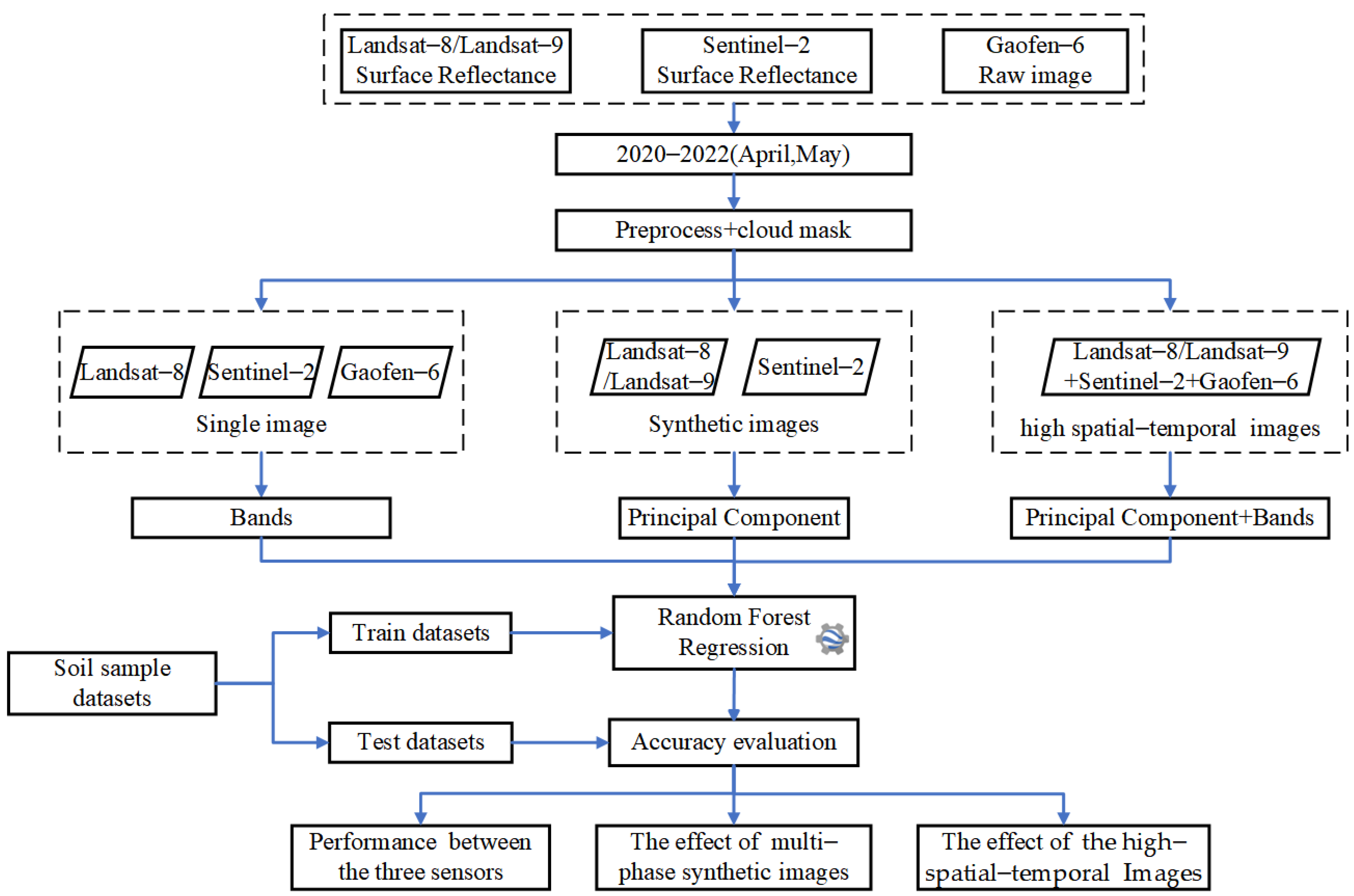
2.6. Technology Framework

The technical framework of this study is shown in Figure 3.
First, we used three satellites to obtain a single-phase image SOM prediction for all images in the study area between 2020 and 2022. Then, the principal components were used as the inputs for the Sentinel-2 and Landsat-8/Lt-9 multi-phase images. Finally, we combined three satellites to construct high spatiotemporal remote sensing images and perform SOM prediction. All predictions were based on the random forest method and the same soil SOM datasets, and the effects of different use methods on SOM prediction were intuitively compared.

3. Results

3.1. Descriptive Statistics of SOM Content in Soil Samples

Descriptive statistics of SOM content of the soil samples used for the study are presented in Table 1. The mean value of measured SOM values for the entire study area was 3.81%, the maximum value was 6.98%, the minimum value was 0.48%, and the standard deviation was 1.21%.

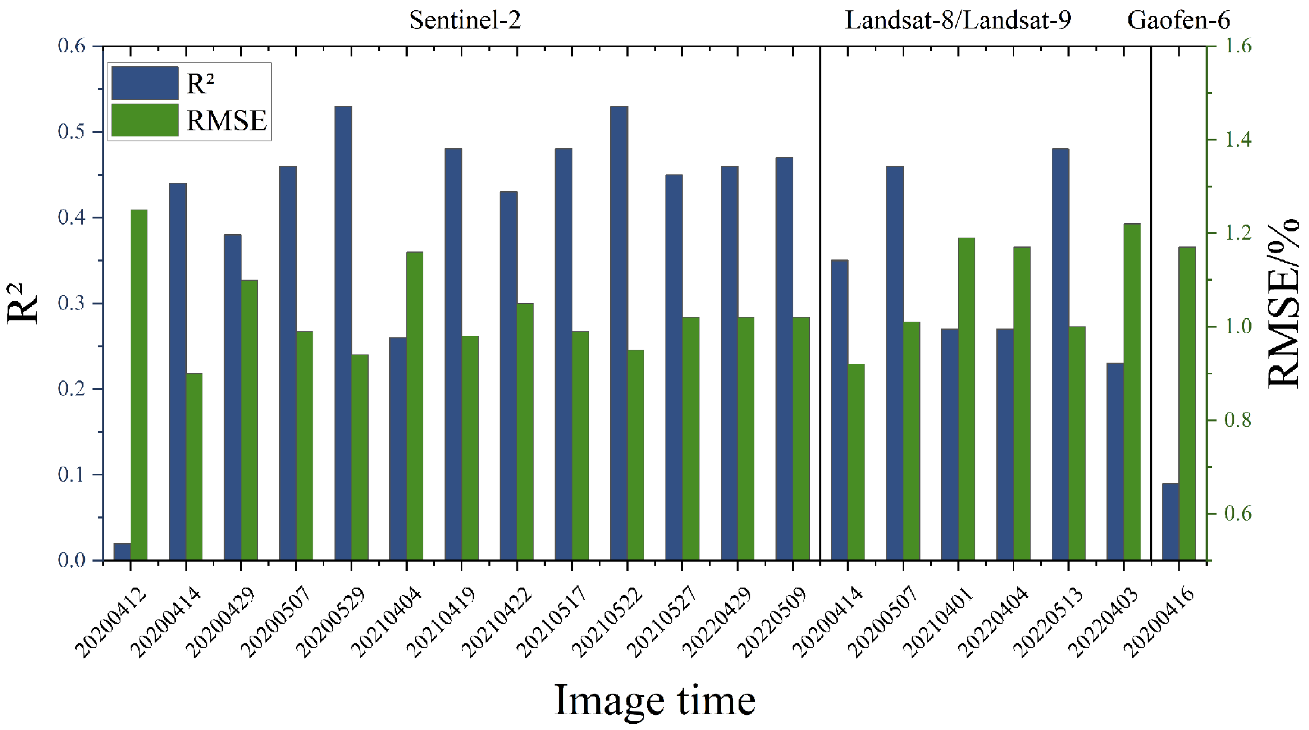
3.2. Predicting SOM Accuracy for Single-Phase Images

This study used all cloud-free images between 1 April and 31 May of each year from 2020 to 2022 for SOM prediction. Although the images used were all cloud-free bare soil period images, their SOM prediction accuracy was still quite different, as shown in Figure 4. R2 ranged from 0.02 to 0.53, and RMSE ranged from 1.25% to 0.94%. Among them, the image with the worst accuracy was the Sentienl-2 image on 12 April 2020, and the image with the highest accuracy was the Sentienl-2 image on 29 May 2020. The average R2 of Sentinel-2 single-phase images was 0.41, and the average R2 of Landsat-8 single-phase images was 0.35. The Gaofen-6 single-phase image, with an imaging date of 16 April 2020, predicted an R2 of SOM of 0.09 and an RMSE of 1.17%.
Among the single-phase images, there were Landsat-8 and Sentinel-2 images obtained on 14 April 2020 and 7 May 2020. Therefore, the prediction capabilities of Landsat-8 and Sentinel-2SOM can be directly compared. For 14 April 2020, Sentienl-2 predicted SOM with an R2 of 0.44 and an RMSE of 0.90%. Landsat-8 predicted SOM with an R2 of 0.35 and a RMSE of 0.92%. For 7 May 2020, Sentienl-2 predicted SOM with an R2 of 0.46 and an RMSE of 0.99%. Landsat-8 predicted SOM with an R2 of 0.46 and a RMSE of 1.01%. The two satellites were well in agreement in predicting SOM.

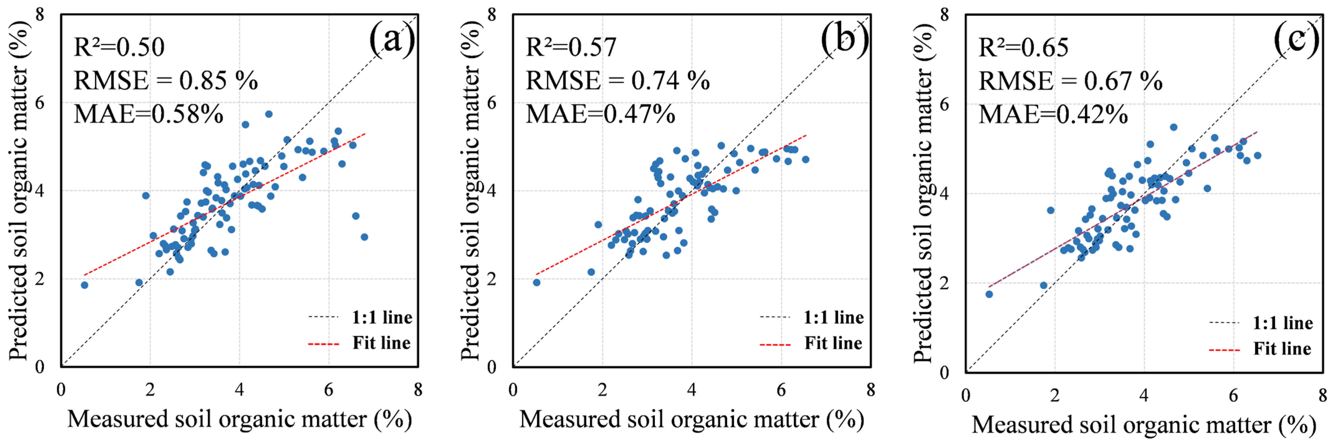
3.3. Predicting SOM Accuracy for Multi-Phase Synthetic Images

The principal components of all Sentinel-2 and Landsat-8/Landsat-9 images were extracted, and a multi-phase synthetic image was constructed based on different sensors. Then, SOM prediction was performed on the multi-phase synthetic images, respectively. As shown in Figure 5, the Sentinel-2 multi-phase synthetic image had an R2 of 0.57 and an RMSE of 0.74%. The Landsat-8/Landsat-9 multi-phase synthetic image had an R2 of 0.50 and RMSE of 0.85%. Sentinel-2 multi-phase synthetic image prediction accuracy was higher. Compared with single-phase images, the SOM prediction accuracy of multi-phase synthetic images from both satellites was significantly improved.
We constructed high spatiotemporal remote sensing images by combining the Sentinel-2 multi-phase synthetic images, Landsat-8/Landsat-9 multi-phase synthetic images, and Gaofen-6 image. The SOM prediction accuracy reached the highest value, with an R2 of 0.65 and RMSE of 0.67%. Compared with the two satellites alone, high spatiotemporal remote sensing images significantly improve SOM prediction accuracy.

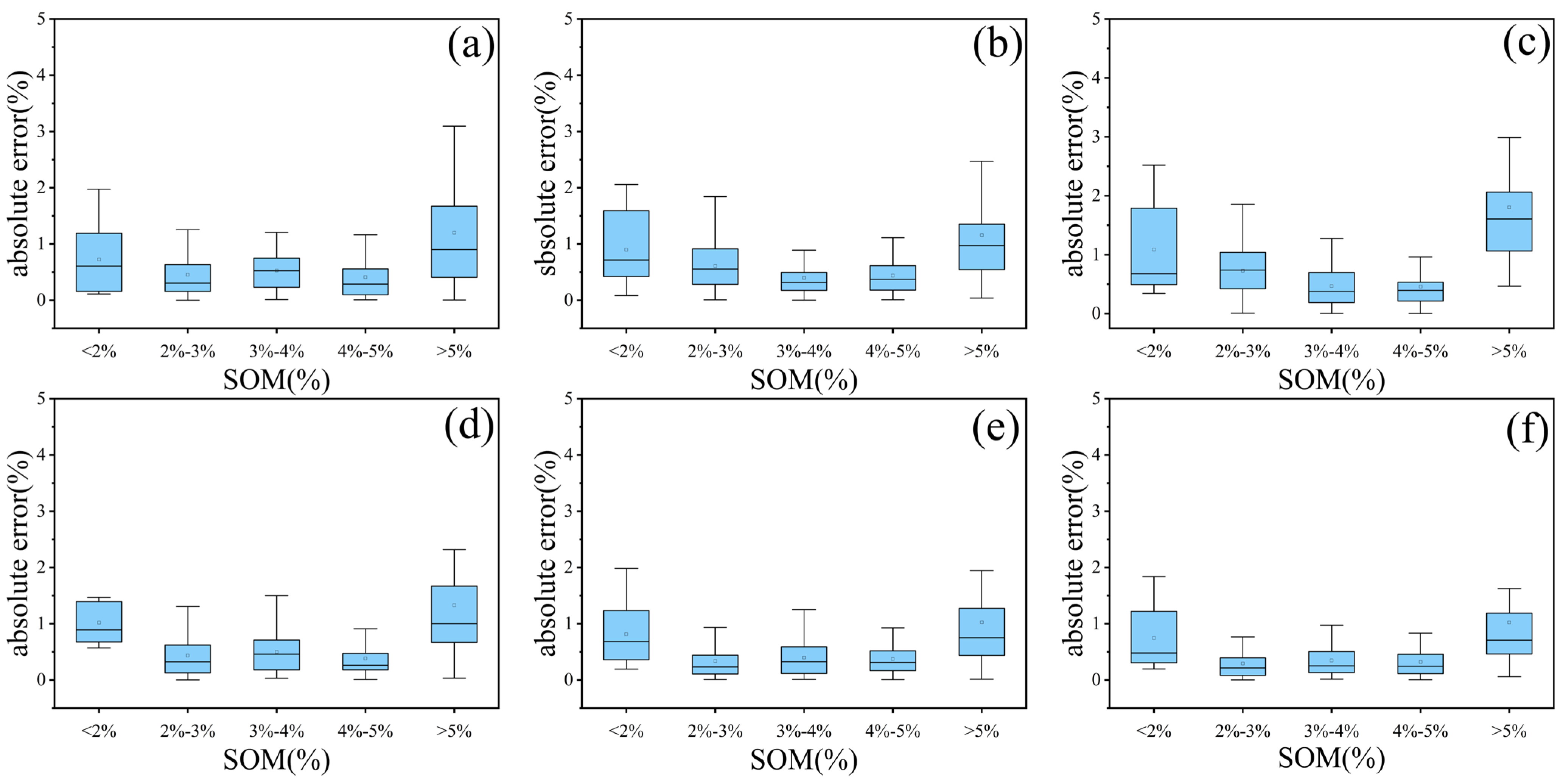
3.4. Absolute Errors in SOM Predictions for Different Ranges

We compared the prediction absolute errors of the single-phase image with the highest prediction accuracy among the three satellites, the two multi-phase synthetic images, and the high spatiotemporal remote sensing images (Figure 6). Among the single-phase images, the Sentinel-2 image had the smallest mean absolute error, followed by the Landsat-8 image, and the Gaofen-6 image had the largest. The average absolute error of Landsat-8 image prediction was the smallest when the SOM was in the low and high-value intervals (<2%; 2–3%; 4–5%). The mean absolute error of the Sentinel-2 image prediction was the smallest when the SOM was in the middle range (3–4%; >5%).
For the high spatiotemporal remote sensing images, the average absolute error was reduced from 0.47% to 0.42% compared with the prediction results of the Sentinel-2 multi-phase synthetic images. The absolute error in the interval with SOM greater than 5% was significantly reduced, and the average absolute error was reduced from 1.00% to 0.86%.

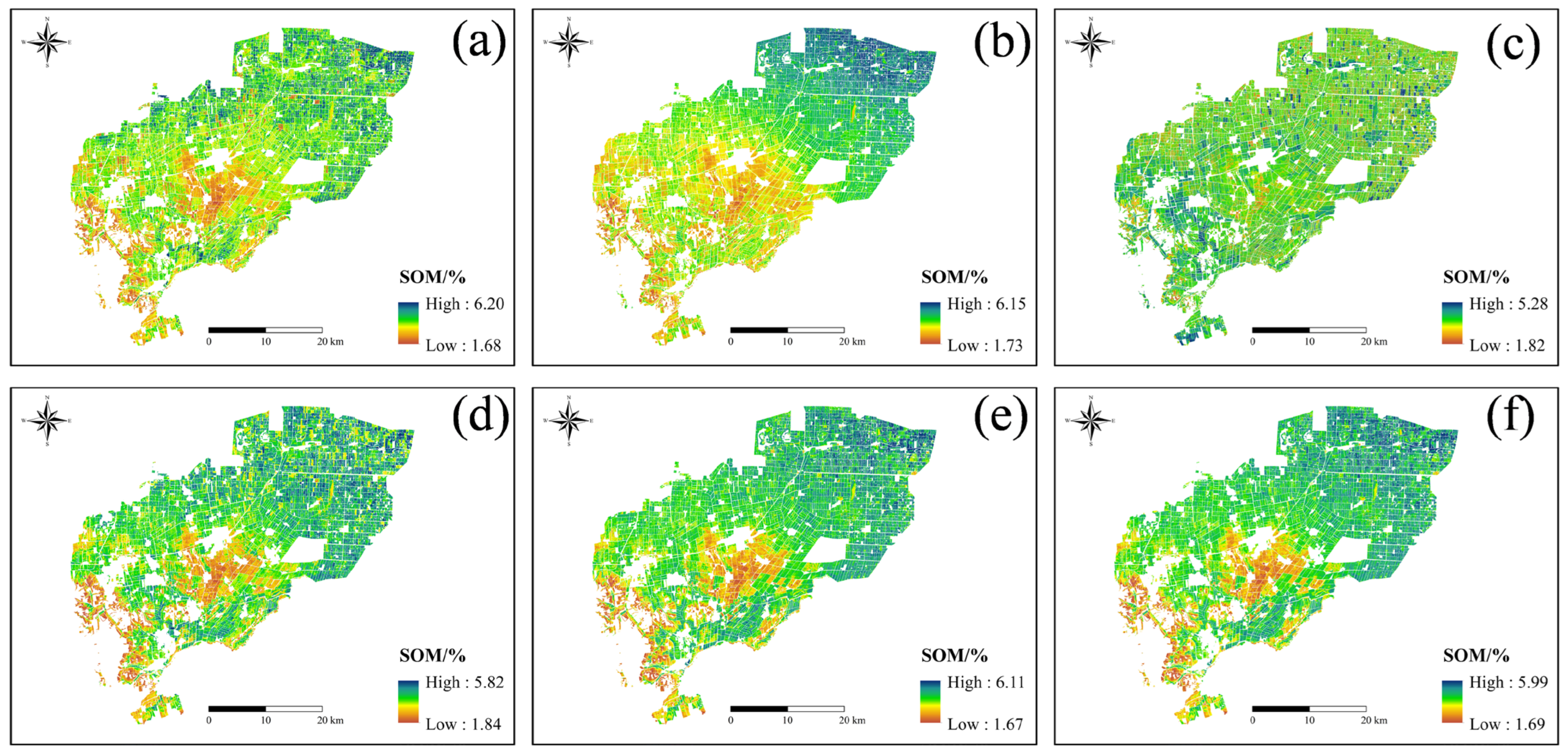
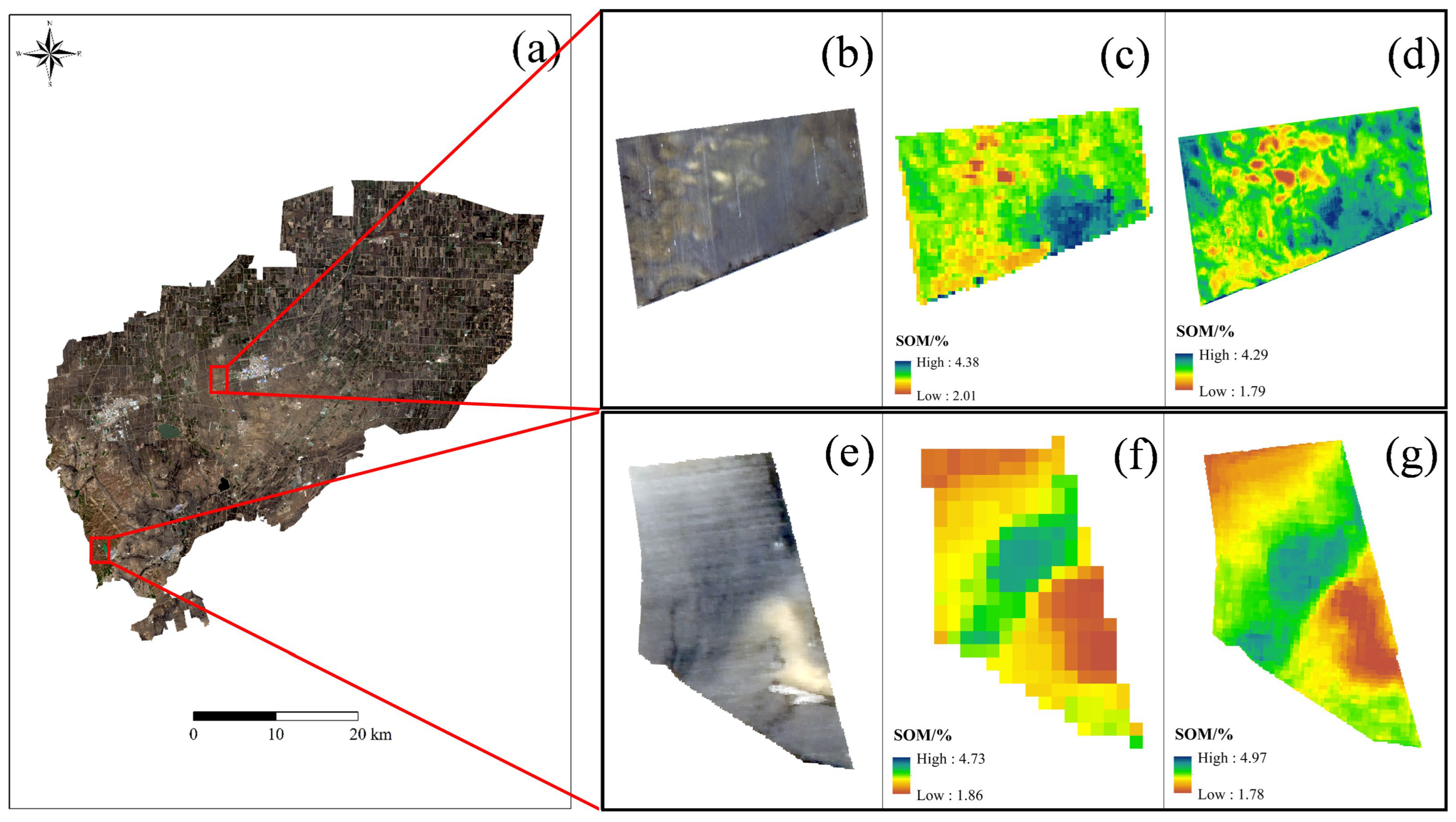
3.5. SOM Prediction Maps

Figure 7 shows the SOM distribution of three satellite single-phase images with the highest accuracy, two multi-phase synthetic images, and high spatiotemporal remote sensing images. The SOM prediction map obtained from single-phase images and multi-phase synthetic images differed in content, but all prediction maps showed the same spatial pattern. The SOM in the eastern part of the study area was significantly higher than that in the central and western parts of the study area. The central and western parts of the study area faced more SOM degradation problems. All SOM prediction maps showed prominent areas of low organic matter values in the central part of the study area. Compared with the significant differences between the SOM prediction results of the single-phase images, the SOM prediction results of multi-phase synthetic images showed better consistency. Finally, the high spatiotemporal remote sensing images prediction result achieved higher prediction accuracy and realized a 2 m spatial resolution, which can show the spatial heterogeneity details of SOM (Figure 7b,f).

4. Discussion

4.1. The Role of High Spatiotemporal Remote Sensing Images for SOM Prediction

High spatiotemporal remote sensing images have apparent advantages over single satellites, one of which is combining the advantages of each satellite to obtain richer and more accurate surface information. For example, in this study, Landsat-8 has an advantage in the spectral response function among the three satellites (Figure 2), Sentinel-2 has more spectral bands, which can obtain more characteristic spectral information, and Gaofen-6 provides 2 m high spatial resolution surface details. Luo’s study shows that multi-phase synthetic images obtained from the same climatic period over multiple years can improve the SOM prediction accuracy compared with single-phase imagery [34]. Meng proposed a new method of SOM prediction by fusing multispectral and hyperspectral satellite data to take advantage of both, and the results proved that multi-source imagery can improve the accuracy of SOM prediction [35]. The Gaofen-6 PMS image has a spatial resolution of 2 m but only four spectral bands. For the characteristic position of SOM after the near-infrared band, 1900 nm [36], 1720 nm, 2180 nm, 2309 nm [37], 1744 nm, 1870 nm, and 2052 nm were obtained [38]. The Gaofen-6 PMS sensor cannot obtain surface spectral information, but it can be comprehensively utilized when combined with Landsat-8 images and Sentinel-2 images, which have short-wave infrared bands. This compensates for the disadvantages of each satellite. Secondly, for the bare soil period, multi-phase images are favorable to reduce the atmospheric cloud disturbances on imaging and the influence of soil moisture and plant residue on SOM Prediction [39]. At the same time, they reduce the imaging interference caused by human activities on cultivated land and obtain more stable soil information [40]. For Northeast China, the bare soil period is long; we can obtain more images during the bare soil period. Comprehensively utilizing multi-phase images can significantly improve SOM prediction accuracy.
In this study, we evaluated the relative importance of the SOM prediction results for each multi-phase synthetic image and high spatiotemporal remote sensing image (Figure 8). We chose to analyze the top five important inputs. The Landsat-8 multi-phase synthetic images have principal components from four images in the top five important inputs. The Sentinel-2 multi-phase synthetic images have principal components from five images in the top five important inputs. In the high spatiotemporal remote sensing images, there are three from Sentinel-2 images and two from Landsat-8 images in the top five important inputs. This shows that multi-source satellites can construct more accurate time-series images to improve SOM prediction accuracy.

4.2. Single Satellite Prediction SOM Comparison

Predicting SOM from remote sensing images, remote sensing data sources, remote sensing data quality, data variables, prediction algorithms, etc., will all affect the SOM prediction accuracy. This study discusses the role of different remote sensing data sources on SOM prediction accuracy. For single-phase images, the results of this study show that the overall prediction accuracy of SOM based on the Gaofen-6 image is lower than that of Landsat-8 and Sentinel-2. For Gaofen-6 images, on the one hand, Gaofen-6 images acquire the spectral reflectance characteristics of SOM in the visible and near-infrared regions due to the small number of bands. The Landsat-8 OLI sensor and Sentinel-2 MSI sensor have more SOM feature bands in the short-wave infrared region, which can obtain more information about the spectral reflectance characteristics of SOM. On the other hand, satellite remote sensing sensors cannot achieve excellent spectral resolution, temporal resolution, and spatial resolution at the same time. The radiometric resolution of Landsat-8, Setinel-2, and Gaofen-6 sensors is 12-bit [41]; the Gaofen-6 PMS sensor achieves a high spatial resolution of 2 m while its spectral response function and radiometric characteristics are weaker than Landsat-8 and Sentinel-2. Lower spatial resolution imaging sensors are advantageous in other aspects of performance, such as improved image signal-to-noise ratio and spectral response function, which improves the SOM prediction accuracy.

4.3. Importance and Application of SOM Mapping at the Meter-Level

The medium spatial resolution represented by Landsat and Sentinel has been widely used in SOM prediction mapping, but its resolution makes it difficult to show the spatial heterogeneity within cropland plots. Soil mapping with higher spatial resolution is an inevitable trend in soil mapping [42]. SOM mapping with meter-level spatial resolution can help to show the correlation between SOM and other elements of arable land, such as topographic features, soil moisture content, crop growth status, and farm yield, which can help us to analyze the relationship between various elements of cropland ecosystem comprehensively [43]. Compared with the results of medium spatial resolution mapping, the results of meter-level spatial resolution SOM mapping can accurately describe the details of highly localized soil-cultivated land, such as depicting the boundaries of degraded cultivated land, which can provide more accurate spatial information for precise management of farmland, reduce the uncertainty of precise management of farmland, and optimize the crop management methods such as fertilizer application and irrigation, to improve the efficiency of agricultural production [44]. For landscapes with strong heterogeneity, finer-resolution images have higher accuracy [45]. In this study, the meter-level resolution results have the same spatial pattern as the medium-resolution results (Figure 7). However, on plots with low SOM value areas caused by sandy soil (Figure 9b) and soil erosion (Figure 9e), the meter-level resolution prediction results can show the SOM spatial heterogeneity details within the plot, and the medium spatial resolution prediction results are difficult to express.

4.4. Limitations and Prospects

This study has proven that high spatiotemporal remote sensing images can effectively improve the SOM prediction accuracy and the spatial resolution of mapping. However, the role of each satellite image in the high spatiotemporal remote sensing images still requires further study. In the future, SOM prediction mapping should pay more attention to the research of multi-sensor collaborative prediction and data fusion to give full play to the advantages of sensors and obtain more accurate surface information from more angles, thereby improving prediction accuracy and spatial resolution.

5. Conclusions

This study evaluated the SOM prediction performance of three satellite images, Landsat-8/Landsat-9, Sentinel-2, and Gaofen-6, and the possibility of using multi-source satellites to construct high spatiotemporal remote sensing images for SOM prediction. The following conclusions were drawn: (1) Sentinel-2 and Landsat-8/Landsat-9 images can be used to extract the principal components of the three-year bare soil period and construct a multi-phase synthetic image. Based on this image, higher SOM prediction accuracy can be obtained than single-phase images, overcoming the instability problem of single-phase images. (2) The highest SOM prediction accuracy can be obtained by constructing high spatiotemporal remote sensing images from three satellite images. (3) The high spatiotemporal remote sensing images also improved spatial resolution to a new level after collaborative analysis with farmland environmental information (soil erosion, low-lying areas, and soil texture), which can determine the causes of abnormal SOM areas. This study emphasized the importance of high spatiotemporal images for SOM prediction. In the future, meter-level SOM mapping results based on this study could provide a new perspective for soil monitoring and promote sustainable soil utilization.

Author Contributions

Conceptualization, Q.M. and H.L.; methodology, C.L.; software, Q.M. and C.L.; validation, C.L. and X.M.; formal analysis, Q.M.; investigation, C.L.; resources, D.Z.; data curation, Q.M.; writing—original draft preparation, Q.M.; writing—review and editing, H.L.; visualization, W.R.; supervision, H.L.; project administration, H.L.; funding acquisition, H.L. All authors have read and agreed to the published version of the manuscript.

Funding

This work was supported by the Jilin Province and the Chinese Academy of Sciences, the Science and Technology Cooperation High-tech Industrialization Special Fund Project (2021SYHZ0013), and the National Key R&D Program of China (2021YFD1500100).

Institutional Review Board Statement

Not applicable.

Informed Consent Statement

Informed consent was obtained from all subjects involved in the study.

Data Availability Statement

Data are available upon request by email to the author.

Conflicts of Interest

The authors declare no conflicts of interest.

References

  1. Franzluebbers, A.J. Soil Organic Matter Stratification Ratio as an Indicator of Soil Quality. Soil Tillage Res. 2002, 66, 95–106. [Google Scholar] [CrossRef]
  2. Rahmani, S.R.; Ackerson, J.P.; Schulze, D.; Adhikari, K.; Libohova, Z. Digital Mapping of Soil Organic Matter and Cation Exchange Capacity in a Low Relief Landscape Using LiDAR Data. Agronomy 2022, 12, 1338. [Google Scholar] [CrossRef]
  3. Nichols, J.D. Relation of Organic Carbon to Soil Properties and Climate in the Southern Great Plains. Soil Sci. Soc. Am. J. 1984, 48, 1382–1384. [Google Scholar] [CrossRef]
  4. Kuzyakov, Y.; Horwath, W.R.; Dorodnikov, M.; Blagodatskaya, E. Chapter Eight—Effects of Elevated CO2 in the Atmosphere on Soil C and N Turnover. In Developments in Soil Science; Horwath, W.R., Kuzyakov, Y., Eds.; Climate Change Impacts on Soil Processes and Ecosystem Properties; Elsevier: Amsterdam, The Netherlands, 2018; Volume 35, pp. 207–219. [Google Scholar]
  5. Liu, Z.; Yang, X.; Hubbard, K.G.; Lin, X. Maize Potential Yields and Yield Gaps in the Changing Climate of Northeast China. Glob. Chang. Biol. 2012, 18, 3441–3454. [Google Scholar] [CrossRef]
  6. Wang, X.; Li, S.; Wang, L.; Zheng, M.; Wang, Z.; Song, K. Effects of Cropland Reclamation on Soil Organic Carbon in China’s Black Soil Region over the Past 35 Years. Glob. Chang. Biol. 2023, 29, 5460–5477. [Google Scholar] [CrossRef] [PubMed]
  7. Orr, H.; Wilby, R.; McKenzie Hedger, M.; Brown, I. Climate Change in the Uplands: A UK Perspective on Safeguarding Regulatory Ecosystem Services. Clim. Res. 2008, 37, 77–98. [Google Scholar] [CrossRef]
  8. Zhou, T.; Geng, Y.; Chen, J.; Liu, M.; Haase, D.; Lausch, A. Mapping Soil Organic Carbon Content Using Multi-Source Remote Sensing Variables in the Heihe River Basin in China. Ecol. Indic. 2020, 114, 106288. [Google Scholar] [CrossRef]
  9. Guo, H.; He, G.; Jiang, W.; Yin, R.; Yan, L.; Leng, W. A Multi-Scale Water Extraction Convolutional Neural Network (MWEN) Method for GaoFen-1 Remote Sensing Images. ISPRS Int. J. Geo-Inf. 2020, 9, 189. [Google Scholar] [CrossRef]
  10. Ottoy, S.; De Vos, B.; Sindayihebura, A.; Hermy, M.; Van Orshoven, J. Assessing Soil Organic Carbon Stocks under Current and Potential Forest Cover Using Digital Soil Mapping and Spatial Generalisation. Ecol. Indic. 2017, 77, 139–150. [Google Scholar] [CrossRef]
  11. Liu, Q.; He, L.; Guo, L.; Wang, M.; Deng, D.; Lv, P.; Wang, R.; Jia, Z.; Hu, Z.; Wu, G.; et al. Digital Mapping of Soil Organic Carbon Density Using Newly Developed Bare Soil Spectral Indices and Deep Neural Network. Catena 2022, 219, 106603. [Google Scholar] [CrossRef]
  12. Demattê, J.A.M.; Alves, M.R.; Terra, F.D.S.; Bosquilia, R.W.D.; Fongaro, C.T.; Barros, P.P.D.S. Is It Possible to Classify Topsoil Texture Using a Sensor Located 800 Km Away from the Surface? Rev. Bras. Ciênc. Solo 2016, 40, e0150335. [Google Scholar] [CrossRef]
  13. Meng, X.; Bao, Y.; Liu, J.; Liu, H.; Zhang, X.; Zhang, Y.; Wang, P.; Tang, H.; Kong, F. Regional Soil Organic Carbon Prediction Model Based on a Discrete Wavelet Analysis of Hyperspectral Satellite Data. Int. J. Appl. Earth Obs. Geoinf. 2020, 89, 102111. [Google Scholar] [CrossRef]
  14. Chen, D.; Chang, N.; Xiao, J.; Zhou, Q.; Wu, W. Mapping Dynamics of Soil Organic Matter in Croplands with MODIS Data and Machine Learning Algorithms. Sci. Total Environ. 2019, 669, 844–855. [Google Scholar] [CrossRef]
  15. Ye, Z.; Sheng, Z.; Liu, X.; Ma, Y.; Wang, R.; Ding, S.; Liu, M.; Li, Z.; Wang, Q. Using Machine Learning Algorithms Based on GF-6 and Google Earth Engine to Predict and Map the Spatial Distribution of Soil Organic Matter Content. Sustainability 2021, 13, 14055. [Google Scholar] [CrossRef]
  16. Zhang, Z.; Lu, L.; Zhao, Y.; Wang, Y.; Wei, D.; Wu, X.; Ma, X. Recent Advances in Using Chinese Earth Observation Satellites for Remote Sensing of Vegetation. ISPRS J. Photogramm. Remote Sens. 2023, 195, 393–407. [Google Scholar] [CrossRef]
  17. Chen, F.; Zhang, W.; Song, Y.; Liu, L.; Wang, C. Comparison of Simulated Multispectral Reflectance among Four Sensors in Land Cover Classification. Remote Sens. 2023, 15, 2373. [Google Scholar] [CrossRef]
  18. Barsi, J.A.; Alhammoud, B.; Czapla-Myers, J.; Gascon, F.; Haque, M.O.; Kaewmanee, M.; Leigh, L.; Markham, B.L. Sentinel-2A MSI and Landsat-8 OLI Radiometric Cross Comparison over Desert Sites. Eur. J. Remote Sens. 2018, 51, 822–837. [Google Scholar] [CrossRef]
  19. Flood, N. Comparing Sentinel-2A and Landsat 7 and 8 Using Surface Reflectance over Australia. Remote Sens. 2017, 9, 659. [Google Scholar] [CrossRef]
  20. Dong, J.; Chen, Y.; Chen, X.; Xu, Q. Radiometric Cross-Calibration of Wide-Field-of-View Cameras Based on Gaofen-1/6 Satellite Synergistic Observations Using Landsat-8 Operational Land Imager Images: A Solution for Off-Nadir Wide-Field-of-View Associated Problems. Remote Sens. 2023, 15, 3851. [Google Scholar] [CrossRef]
  21. Guo, L.; Liu, Y.; He, H.; Lin, H.; Qiu, G.; Yang, W. Consistency Analysis of GF-1 and GF-6 Satellite Wide Field View Multi-Spectral Band Reflectance. Optik 2021, 231, 166414. [Google Scholar] [CrossRef]
  22. Li, R.; Wang, L.; Lu, Y. A Comparative Study on Intra-Annual Classification of Invasive Saltcedar with Landsat 8 and Landsat 9. Int. J. Remote Sens. 2023, 44, 2093–2114. [Google Scholar] [CrossRef]
  23. Shi, J.; Shen, Q.; Yao, Y.; Li, J.; Chen, F.; Wang, R.; Xu, W.; Gao, Z.; Wang, L.; Zhou, Y. Estimation of Chlorophyll-a Concentrations in Small Water Bodies: Comparison of Fused Gaofen-6 and Sentinel-2 Sensors. Remote Sens. 2022, 14, 229. [Google Scholar] [CrossRef]
  24. Xia, C.; Zhang, Y. Comparison of the Use of Landsat 8, Sentinel-2, and Gaofen-2 Images for Mapping Soil pH in Dehui, Northeastern China. Ecol. Inform. 2022, 70, 101705. [Google Scholar] [CrossRef]
  25. Zhang, M.; Lin, H. Wetland Classification Using Parcel-Level Ensemble Algorithm Based on Gaofen-6 Multispectral Imagery and Sentinel-1 Dataset. J. Hydrol. 2022, 606, 127462. [Google Scholar] [CrossRef]
  26. Li, Q.; Wang, L.; Fu, Y.; Lin, D.; Hou, M.; Li, X.; Hu, D.; Wang, Z. Transformation of Soil Organic Matter Subjected to Environmental Disturbance and Preservation of Organic Matter Bound to Soil Minerals: A Review. J. Soils Sediments 2023, 23, 1485–1500. [Google Scholar] [CrossRef]
  27. Hu, L.; Li, Q.; Yan, J.; Liu, C.; Zhong, J. Vegetation Restoration Facilitates Belowground Microbial Network Complexity and Recalcitrant Soil Organic Carbon Storage in Southwest China Karst Region. Sci. Total Environ. 2022, 820, 153137. [Google Scholar] [CrossRef]
  28. Chander, G.; Helder, D.L.; Aaron, D.; Mishra, N.; Shrestha, A.K. Assessment of Spectral, Misregistration, and Spatial Uncertainties Inherent in the Cross-Calibration Study. IEEE Trans. Geosci. Remote Sens. 2013, 51, 1282–1296. [Google Scholar] [CrossRef]
  29. Grimm, R.; Behrens, T.; Märker, M.; Elsenbeer, H. Soil Organic Carbon Concentrations and Stocks on Barro Colorado Island—Digital Soil Mapping Using Random Forests Analysis. Geoderma 2008, 146, 102–113. [Google Scholar] [CrossRef]
  30. Schulze, D.G.; Nagel, J.L.; Van Scoyoc, G.E.; Henderson, T.L.; Baumgardner, M.F.; Stott, D.E. Significance of Organic Matter in Determining Soil Colors. In Soil Color; Wiley: Hoboken, NJ, USA, 1993. [Google Scholar]
  31. Belgiu, M.; Drăguţ, L. Random Forest in Remote Sensing: A Review of Applications and Future Directions. ISPRS J. Photogramm. Remote Sens. 2016, 114, 24–31. [Google Scholar] [CrossRef]
  32. Gorelick, N.; Hancher, M.; Dixon, M.; Ilyushchenko, S.; Thau, D.; Moore, R. Google Earth Engine: Planetary-Scale Geospatial Analysis for Everyone. Remote Sens. Environ. 2017, 202, 18–27. [Google Scholar] [CrossRef]
  33. Hamzehpour, N.; Shafizadeh-Moghadam, H.; Valavi, R. Exploring the Driving Forces and Digital Mapping of Soil Organic Carbon Using Remote Sensing and Soil Texture. Catena 2019, 182, 104141. [Google Scholar] [CrossRef]
  34. Luo, C.; Zhang, W.; Zhang, X.; Liu, H. Mapping of Soil Organic Matter in a Typical Black Soil Area Using Landsat-8 Synthetic Images at Different Time Periods. Catena 2023, 231, 107336. [Google Scholar] [CrossRef]
  35. Meng, X.; Bao, Y.; Wang, Y.; Zhang, X.; Liu, H. An Advanced Soil Organic Carbon Content Prediction Model via Fused Temporal-Spatial-Spectral (TSS) Information Based on Machine Learning and Deep Learning Algorithms. Remote Sens. Environ. 2022, 280, 113166. [Google Scholar] [CrossRef]
  36. Palacios-Orueta, A.; Ustin, S.L. Remote Sensing of Soil Properties in the Santa Monica Mountains I. Spectral Analysis. Remote Sens. Environ. 1998, 65, 170–183. [Google Scholar] [CrossRef]
  37. Shepherd, K.D.; Walsh, M.G. Division S-8—Nutrient Management & Soil & Plant Analysis. Soil. Sci. Soc. Am. J. 2002, 66, 268–275. [Google Scholar]
  38. Dalal, R.C.; Henry, R.J. Simultaneous Determination of Moisture, Organic Carbon, and Total Nitrogen by Near Infrared Reflectance Spectrophotometry. Soil Sci. Soc. Am. J. 1986, 50, 120–123. [Google Scholar] [CrossRef]
  39. Dou, X.; Wang, X.; Liu, H.; Zhang, X.; Meng, L.; Pan, Y.; Yu, Z.; Cui, Y. Prediction of Soil Organic Matter Using Multi-Temporal Satellite Images in the Songnen Plain, China. Geoderma 2019, 356, 113896. [Google Scholar] [CrossRef]
  40. Luo, C.; Zhang, X.; Meng, X.; Zhu, H.; Ni, C.; Chen, M.; Liu, H. Regional Mapping of Soil Organic Matter Content Using Multitemporal Synthetic Landsat 8 Images in Google Earth Engine. Catena 2022, 209, 105842. [Google Scholar] [CrossRef]
  41. Niroumand-Jadidi, M.; Bovolo, F.; Bresciani, M.; Gege, P.; Giardino, C. Water Quality Retrieval from Landsat-9 (OLI-2) Imagery and Comparison to Sentinel-2. Remote Sens. 2022, 14, 4596. [Google Scholar] [CrossRef]
  42. Zeraatpisheh, M.; Jafari, A.; Bagheri Bodaghabadi, M.; Ayoubi, S.; Taghizadeh-Mehrjardi, R.; Toomanian, N.; Kerry, R.; Xu, M. Conventional and Digital Soil Mapping in Iran: Past, Present, and Future. Catena 2020, 188, 104424. [Google Scholar] [CrossRef]
  43. Wadoux, A.M.J.; Román Dobarco, M.; Malone, B.; Minasny, B.; McBratney, A.B.; Searle, R. Baseline High-Resolution Maps of Organic Carbon Content in Australian Soils. Sci. Data 2023, 10, 181. [Google Scholar] [CrossRef] [PubMed]
  44. Ahmad, U.; Sharma, L. A Review of Best Management Practices for Potato Crop Using Precision Agricultural Technologies. Smart Agric. Technol. 2023, 4, 100220. [Google Scholar] [CrossRef]
  45. Piedallu, C.; Pedersoli, E.; Chaste, E.; Morneau, F.; Seynave, I.; Gégout, J.-C. Optimal Resolution of Soil Properties Maps Varies According to Their Geographical Extent and Location. Geoderma 2022, 412, 115723. [Google Scholar] [CrossRef]
Figure 1. Schematic diagram of the location of the study area, soil map, and sampling points.
Sustainability 16 01497 g001
Figure 2. Spectral response functions (SRF) of three sensors in five bands. (a) Blue band. (b) Green band. (c) Red band. (d) Near-infrared band. (e) Panchromatic band.
Sustainability 16 01497 g002
Figure 3. The technology framework for constructing a meter-level SOM prediction model using Sentinel-2, Landsat-8/9, and Gaofen-6 data.
Sustainability 16 01497 g003
Figure 4. Accuracy of predicting SOM using different satellites, different imaging dates, and single-phase images.
Sustainability 16 01497 g004
Figure 5. Comparison of predicted SOM and measured SOM for multi-phase synthetic images and high spatiotemporal remote sensing images. (a) Landsat-8/Landsat-9 multi-phase synthetic images; (b) Sentinel-2 multi-phase synthetic images; (c) high spatiotemporal remote sensing images.
Sustainability 16 01497 g005
Figure 6. Boxplot of absolute error for different SOM intervals. (a) Landsat-8 single-phase image; (b) Sentinel-2 single-phase image; (c) Gaofen-6 single-phase image; (d) Landsat-8/Landsat-9 multi-phase synthetic images; (e) Sentinel-2 multi-phase synthetic images; (f) high spatiotemporal remote sensing images.
Sustainability 16 01497 g006
Figure 7. SOM prediction maps based on different image inputs. (a) Landsat-8 single-phase image; (b) Sentinel-2 single-phase image; (c) Gaofen-6 single-phase image; (d) Landsat-8/Landsat-9 multi-phase synthetic images; (e) Sentinel-2 multi-phase synthetic images; (f) high spatiotemporal remote sensing images.
Sustainability 16 01497 g007
Figure 8. The top five important inputs of each multi-phase synthetic image and high spatiotemporal remote sensing images. (a) Landsat-8/Landsat-9 multi-phase synthetic images; (b) Sentinel-2 multi-phase synthetic images; (c) high spatiotemporal remote sensing images.
Sustainability 16 01497 g008
Figure 9. Comparison of SOM prediction results for two typical plots. (a) Location of two typical plots; (b) RGB image of the sandy soil plot; (c) Landsat-8/Landsat-9 multi-phase synthetic images result; (d) high spatiotemporal remote sensing images result; (e) RGB image of the soil erosion plot; (f) Landsat-8/Landsat-9 multi-phase synthetic images result; (g) high spatiotemporal remote sensing images result.
Sustainability 16 01497 g009
Table 1. Statistical description of SOM content in soil samples.
DatasetNMax/%Min/%Mean/%SD/%
Whole set2796.980.483.811.21
Training set1866.980.483.811.21
Validation set936.800.533.811.22
Note: N—number of samples; SD—standard deviation.
Disclaimer/Publisher’s Note: The statements, opinions and data contained in all publications are solely those of the individual author(s) and contributor(s) and not of MDPI and/or the editor(s). MDPI and/or the editor(s) disclaim responsibility for any injury to people or property resulting from any ideas, methods, instructions or products referred to in the content.

