Research on the Evaluation and Influencing Factors of China’s Provincial Employment Quality Based on Principal Tensor Analysis

Abstract

The research on the quality of employment in China holds immense significance for attaining high-quality employment development. Firstly, enhancing the quality of employment facilitates the optimization of labor resource allocation and enhances economic efficiency. Secondly, high-quality employment serves as a fundamental pillar for social equity and stability. Lastly, continual enhancement of employment quality caters to the requirements of social development and plays a crucial role in promoting economic transformation and achieving sustainable development. However, what is the current situation of employment quality in China? How can we scientifically measure employment quality? What are the key factors for the development of employment quality? This study aimed to use spatiotemporal tensor data to measure the level of employment quality in China’s provinces and analyzed the magnitude and direction of its influencing factors in the spatiotemporal dimension. Taking thirty provinces, autonomous regions, and municipalities directly under the central government in China from 2011 to 2020 as the research objects, the employment quality evaluation system was constructed from six dimensions: employment environment, employment status, employability, labor remuneration, social security, and labor relations. The employment quality index data were expressed in the form of three-order, high-dimensional tensor spatiotemporal data, and the employment quality of China’s provinces was measured from the spatiotemporal perspective by using principal tensor analysis. Then, the visual analysis of the development and change process of employment quality was carried out. The spatial autocorrelation analysis of employment quality was carried out, and the time–space dual-fixed-effect model of the spatial Durbin model was selected to analyze the direction and magnitude of the influence factors of employment quality on the selected and neighboring provinces. The research showed that: (1) The overall level of employment quality in China was not high, the employment quality varied greatly among provinces, and the employment quality development gap among provinces showed a trend of widening. (2) The development of employment quality in western China was relatively fast, while the development of employment quality in central China showed insufficient stamina. (3) Sichuan Province had a strong radiation effect on the development of employment quality in neighboring provinces, and Beijing and Tianjin had a strong siphon effect on the development of employment quality in neighboring provinces. (4) The level of industrialization and informatization promoted the development of employment quality in China’s provinces, while the industrial structure had a significant negative effect on the development of employment quality. According to the research findings, the following policy recommendations are proposed: (1) strengthen inter-provincial cooperation and exchange, (2) emphasize support for the central and western regions, (3) fully leverage the radiation effect of Sichuan while optimizing the siphon effect of Beijing and Tianjin, and (4) enhance industrialization and information technology levels, as well as adjust the industrial structure.

1. Introduction

The 20th National Congress of the Communist Party of China pointed out that employment supports the basic livelihood of the people and there is a need to strengthen employment policy priorities, improve the mechanism of employment, and promote high-quality full employment. China’s 14th Five-Year Development Plan and 2035 long-term goals require improving the promotion mechanism that is conducive to more sufficient and higher-quality employment, expanding employment capacity, improving employment quality, and alleviating structural employment contradictions. The Chinese government attaches great importance to people’s livelihood and well-being and strives to promote both the quality and quantity of employment development. The quality of employment is closely related to China’s sustainable development. Firstly, high-quality employment can help promote sustainable economic development. When workers have sufficient knowledge and skills and engage in competitive industries, they can create more economic value and promote economic growth. At the same time, a stable employment environment provides workers with a stable income source, stimulating consumption and demand, and further promoting economic development. Secondly, high-quality employment can help develop and utilize human resources. By providing a good working environment and vocational training, it can enhance the skills and knowledge level of workers and promote personal development and social progress. At the same time, high-quality employment can attract more talents to come to China and inject new vitality into China’s sustainable development. In addition, high-quality employment can help protect the environment. For example, providing employment opportunities in renewable energy and green industries can promote the development of the environmental protection industry, reducing pollution and damage to the environment. At the same time, providing environmental education and training can help workers establish environmental awareness and promote green sustainable development of society. Therefore, there is a close correlation between China’s employment quality and sustainable development. By improving the quality of employment, we can promote economic prosperity and social stability, and achieve the Sustainable Development Goals. Therefore, the government, enterprises, and workers need to work together to create a good employment environment, improve employment quality, and promote China’s sustainable development. At present, China’s economic growth rate has dropped from 10% to about 7%, and economic development is an important support for ensuring employment and people’s livelihood. In the context of slowing economic growth, how can we ensure the quality and quantity of employment? How can we scientifically measure the quality of employment? What are the key factors in the development of employment quality? China is the largest developing country in the world, with the largest population and a large population density. China’s national conditions have their own particularities and compatibility. Firstly, there are imbalances in China’s industrial development level, education distribution, industrial structure distribution, and digital innovation distribution. Secondly, there is a large difference in economic development between the east and west of China, and the supporting industries for economic development are different, resulting in significant differences in time and space. Therefore, it is more scientifically significant to study China’s employment quality from a temporal and spatial perspective.

2. Literature Review

2.1. Research on the Measurement of Employment Quality

Grossmann V. summarized that the European Union’s research on employment quality mainly focuses on two aspects: labor market and employment characteristics [1]. Arranz J. M et al. measured employment quality in three dimensions: working conditions, skills and training, and work–life balance [2]. Chreneková M. et al. conducted decent work into the employment quality evaluation system [3]. Some scholars also used questionnaires to eliminate unreasonable indicators in the employment quality evaluation system [4,5]. Ming J. built an employment quality evaluation system with four dimensions, including income, working hours, labor contract, and social security, and measured the employment quality of migrant workers through a multi-dimensional employment quality index [6]. Li N. analyzed the existing employment quality index system and provided statistical suggestions on employment quality [7]. Mao J. J. et al. built an evaluation system with four dimensions: income, working hours, labor contracts, and social security, and measured the employment quality index by the equal-weighted average method [8]. Ling L. also constructed an employment quality evaluation system with four dimensions: income level, working hours, social security, and employment satisfaction, and calculated the employment quality index through CRITIC empowerment [9].

In the research on employment quality evaluation, there is no scientific explanation for the construction of an employment quality evaluation system. When measuring employment quality, the traditional principal component analysis and entropy value methods are mostly used. These methods can only measure employment quality in the time dimension and do not support the comprehensive measurement of employment quality in the time and space dimension. The present study employs quantitative analysis to assess employment quality, enabling the comprehensive exploration of multi-dimensional and multi-featured interactions, as well as facilitating feature extraction, dimension reconstruction, and visualization of spatiotemporal employment data. Consequently, this study pioneers the application of principal tensor analysis for constant-order dimensionality reduction in a three-order, high-dimensional evaluation system for employment quality, thereby allowing the measurement of China’s provincial employment quality score using spatiotemporal tensor data.

2.2. Research on Factors Affecting Employment Quality

Scholars use different methods to measure factors affecting employment quality from different angles. Chen G. S. et al. analyzed the impact of human capital investment on rural non-agricultural employment in Hunan Province based on time series data [10]. Yang Y. L. et al. used impulse response analysis to test the impact of the urbanization level on employment quality in China [11]. Zheng H. L. et al. measured the correlation between employment structure, industrial structure, and economic growth [12]. Ma R. studied the impact of government fiscal expenditure on labor employment by constructing a spatial Durbin model [13]. Sheng Y. N. studied the impact of fertility policy adjustments on women’s employment quality through the double-difference method [14]. Xie M. M. et al. analyzed the impact of artificial intelligence and technological progress on low-skilled employment in manufacturing [15]. Zhou C. used the endogenous transformation model to analyze the impact of government training on the employment of migrant workers [16]. Zhang M. Z. et al. studied the impact of external tariff changes on regional labor employment in China [17].

The research on the factors affecting the quality of employment mainly analyzes how the factors affect the quality while ignoring the spatial correlation; that is, ignoring the effects of the factors affecting the quality of employment in neighboring provinces. The spatial econometric model is employed in this study to analyze the determinants of employment quality across China’s provinces. From a temporal perspective, this model enables us to examine the impacts and pathways through which employment quality factors influence both the selected province and its neighboring regions.

The research objects of this paper are 30 provinces, autonomous regions, and municipalities (hereinafter referred to as provinces) in China, excluding Tibet Autonomous Region, Hong Kong, Macao, and Taiwan. We collected employment quality-related index data from 30 provinces in China from 2011 to 2020 and organized and constructed third-order, high-dimensional data of the employment quality evaluation index system based on the tensor structure. The Principal Tensor Analysis 3 model was used to analyze the employment quality evaluation index system. Through the fiber operation and slice operation of the tensor, the dimensional reconstruction feature analysis and visual expression of the index system were carried out. We explored the spatial correlation of provincial employment quality and established a spatial econometric model to analyze the magnitude and direction of the impact of each province’s employment development on the economic and social development of the selected and neighboring provinces, thereby providing data support and theoretical support for the government and enterprises to formulate policies.

3. Research Methods

The purpose of this study was to use spatiotemporal data to measure China’s provincial employment quality, further determine the spatial correlation of China’s provincial employment quality, and determine the size and direction of the factors affecting employment quality [18]. (1) The PTA3 method was designed to decompose the comprehensive interaction of multi-dimensions and multi-features and could reduce the dimensionality of high-order and high-dimensional data without changing their order. It overcomes the disadvantage of processing spatiotemporal multi-dimensional data in a sequential manner while ignoring its multilinear structure. Therefore, this study applied the PTA3 method to measure employment quality from a spatiotemporal perspective for the first time, making up for the shortcomings of existing research that ignored the comprehensive role of multi-dimensional and multi-feature data in the employment quality evaluation system. (2) Global spatial autocorrelation was selected to analyze the spatial correlation of employment quality. (3) The spatial econometric model could analyze the direction and magnitude of the impact of factors affecting employment quality on the selected and neighboring provinces from a spatial perspective.

3.1. PTAk Model of k-Order Tensor (K > 2)

PTAk is a method of decomposing high-dimensional array data; that is, N (N > 2)-order tensors. It is a high-dimensional extension of principal component analysis. It uses low-order tensors to approximate high-order tensors, thereby realizing feature extraction for high-dimensional data. PTAk is essentially a generalized singular value decomposition model and uses the alternating least squares method to achieve the calculation of the principal tensor. The orthogonal sub-tensor of the original tensor can be effectively obtained to approximate the high-dimensional space, and the reliability test and selection of the principal tensor can be performed based on the size of the singular value. For a long time, for the processing of spatiotemporal multi-dimensional data, they are often converted into vectors in order and analyzed in the linear subspace. Treating spatiotemporal multi-dimensional data in an ordinal manner often ignores the multilinear structure. Similar to a bidirectional analysis table, a multidirectional analysis table must be collapsed or expanded in a table with two modes, thus looking at second-order interactions in multiple ways, rather than looking at multiple interactions. The framework used by the PTAk model extends some duality principles and thus extends the multi-dimensional analysis approach focusing on spatiotemporal data. The form of the PTAk model for a k-order tensor is as follows:

The first principal quantity, the optimized form of a singular value, is as follows:

$$\begin{gathered} {\sigma }_1=maxX..\left(\psi \otimes \phi \otimes \varphi \right) \\ {\left|\right|\psi \left|\right|}_s=1 \\ {\left|\right|\phi \left|\right|}_v=1 \\ {\left|\right|\varphi \left|\right|}_t=1 \\ =X({\psi }_1\otimes {\phi }_1\otimes {\varphi }_1) \end{gathered}$$

(1)

Among them, “⨂” represents the tensor product, “..” indicates the contraction operation, which is equivalent to the inner product operation of the tensor space, X represents matrix data or tensor data of the same data table, ${\psi }_1, {\phi }_1, { \varphi }_1$ are the first principal components, and ${\psi }_1\otimes {\phi }_1\otimes {\varphi }_1$ is called the first principal component. From this, the best rank-one approximation and singular value of a given tensor X can be calculated. The calculation method of this step is called the RPVSCC algorithm. It is equivalent to TUCKALS3, which takes only one component per modulo. The proof of the uniqueness of the tensor solution provided by Equation (1) under orthogonal transformation was presented by Leibovici in 1998 [18].

The calculation of the PTAk model is more convenient, because it does not directly calculate the tensor product of vectors by algebraic methods, but executes the contraction operator, as shown in Equation (2):

$$\begin{gathered} X..\left(\psi \otimes \phi \otimes \varphi \right)=\left(X..\psi \right)..\left(\phi \otimes \varphi \right) \\ =(X..\phi )..(\psi \otimes \varphi ) \\ =(X..\phi )..(\psi \otimes \phi ) \\ =\left(\right(X..\psi )..\phi )..\varphi \end{gathered}$$

(2)

If an orthogonality constraint is added to Equation (1), the second a principal tensor can be solved, the optimization process equivalent to the previous step in the solution process acts on the projection $P_{({\psi }_1^{\perp }\otimes {\phi }_1^{\perp }\otimes {\varphi }_1^{\perp })}X$ of the tensor X on the orthogonal tensor of the first argument, where ${\psi }_1^{\perp }\otimes {\phi }_1^{\perp }\otimes {\varphi }_1^{\perp }$ represents the orthogonal tensor of the first principal tensor, which can also be written as $(Id-P_{{\psi }_1})\otimes (Id-P_{{\phi }_1})\otimes (Id-P_{{\varphi }_1})$.

According to the algorithm pattern in Equation (3), PTAk decomposition yields a method of synthesizing data from the set of uncorrelated components. In the schemas implemented for the PTA3(X) and PTAk(X) functions, it is possible to distinguish between the principal tensor and associated principal tensor. The latter are related to principal tensor because they display one or more components of this principal tensor in the first principal tensor’s component set. After a tensor of rank k performs a contraction operator on a given component, the associated principal tensor quantity can be decomposed by PTA(k − 1). This makes the PTAk algorithm a recursive algorithm. When k = 3, there are:

$$\begin{gathered} \mathrm{P}\mathrm{T}\mathrm{A}3\left(\mathrm{X}\right)={\mathsf{\sigma }}_1\left({\mathrm{\psi }}_1\otimes {\mathsf{\phi }}_1\otimes {\mathsf{\varphi }}_1\right)+{\mathrm{\psi }}_1{\otimes }_{1}PTA2\left(P\left({\phi }_1^{\perp }\otimes {\varphi }_1^{\perp }\right)\left(X..{\psi }_1^{\perp }\right)\right)+{\mathsf{\phi }}_1{\otimes }_{2}PTA2\left(P\left({\psi }_1^{\perp }\otimes {\varphi }_1^{\perp }\right)\left(X..{\phi }_1^{\perp }\right)\right) \\ +{\mathsf{\varphi }}_1{\otimes }_{3}PTA2\left(P\left({\psi }_1^{\perp }\otimes {\phi }_1^{\perp }\right)\left(X..{\varphi }_1^{\perp }\right)\right)+PTA3\left(P\left({\psi }_1^{\perp }\otimes {\phi }_1^{\perp }\otimes {\varphi }_1^{\perp }\right)X\right) \end{gathered}$$

(3)

The notation ${\otimes }_1$ means that in this full tensor product operation, the vector on the left will occupy the ith position in k positions, such as ${\mathsf{\phi }}_1{\otimes }_2(\mathsf{\alpha }\otimes \mathsf{\beta })=\mathsf{\alpha }\otimes {\mathsf{\phi }}_1\otimes \mathsf{\beta }$.

PTA3 Model Algorithm

Before introducing the algorithm of the PTAk model, the RPVSCC algorithm is explained first. The goal of the RPVSCC algorithm is to find the principal tensor quantity of the initial tensor X, and its pseudocode is as follows (Algorithm 1):

Algorithm 1. RPVSCC Algorithm (k = 3)

Input: Tensor X, maximum iteration step size MAX, and stop iteration threshold ε Output: singular value σ and its principal tensor components α, β, γ Step: 1: Initialize a set of principal tensor components ${\alpha }_0$$, {\beta }_0$$, {\gamma }_0$ 2: For i from 1 to MAX: $\hspace{1em}\hspace{1em}\hspace{1em}\hspace{1em}\hspace{1em}\hspace{1em}\hspace{1em}\hspace{1em}\hspace{1em}\hspace{1em}\hspace{1em}\hspace{1em}\hspace{1em}\hspace{1em}(X..{\beta }_{i-1})..{\gamma }_{i-1}={\sigma }_i^{\alpha }{\alpha }_i$ $\hspace{1em}\hspace{1em}\hspace{1em}\hspace{1em}\hspace{1em}\hspace{1em}\hspace{1em}\hspace{1em}\hspace{1em}\hspace{1em}\hspace{1em}\hspace{1em}\hspace{1em}\hspace{1em}\hspace{1em}(X..{\gamma }_{i-1})..{\alpha }_i={\sigma }_i^{\beta }{\beta }_i$ $\hspace{1em}\hspace{1em}\hspace{1em}\hspace{1em}\hspace{1em}\hspace{1em}\hspace{1em}\hspace{1em}\hspace{1em}\hspace{1em}\hspace{1em}\hspace{1em}\hspace{1em}\hspace{1em}\hspace{1em}\hspace{1em}(X..{\alpha }_i)..{{\beta }_i}_i={\sigma }_i^{\gamma }{\gamma }_i$ If the extreme value of ${\sigma }_i^{\alpha }$$, {\sigma }_i^{\beta }$$, {\sigma }_i^{\gamma }$ is less than ε jump out of the iteration loop and output ${\sigma }_i$$, {\alpha }_i$$, {\beta }_i$$, {\gamma }_i$.

The pseudocode of the complete PTAk algorithm is as follows (Algorithm 2):

Algorithm 2. PTAk Algorithm (k = 3)

Input: tensor X, order k = 3, maximum iteration step size MAX, and stop iteration threshold ε Output: principal tensor $A_i$, i $=1,2,\cdots$, m, associated principal tensor $A_i^j$, j $=1,2,\cdots$,k Step: 1: Run the RPVSCC algorithm to obtain the principal tensor $A_i=S_i^1\otimes S_i^2\otimes \cdots \otimes S_i^k$ 2: On the orthogonal tensor space of the solution obtained in step 1, continue with step 1 to obtain all m principal tensors 3: For i from 1 to m:    For j from 1 to k: $\hspace{1em}\hspace{1em}\hspace{1em}\hspace{1em}\hspace{1em}\hspace{1em}\hspace{1em}\hspace{1em}\hspace{1em}\hspace{1em}\hspace{1em}\hspace{1em}\hspace{1em}\hspace{1em}\hspace{1em}\hspace{1em}{X}_i^j=X..S_i^j$ $\hspace{1em}\hspace{1em}\hspace{1em}\hspace{1em}\hspace{1em}\hspace{1em}\hspace{1em}\hspace{1em}\hspace{1em}\hspace{1em}\hspace{1em}\hspace{1em}\hspace{1em}\hspace{1em}{A}_i^j=PTA(k-1)\ast X_i^j$ $\mathrm{Return} { A}_i^j$

In the pseudocode of the PTAk algorithm, for a fixed i and j, $A_i^j$ does not necessarily represent only an associated principal tensor quantity because the $PTA(k-1)\ast X_i^j$ optimization may select multiple association principal tensors. Moreover, the singular value of each principal tensor quantity obtained is not necessarily larger than the singular value of all associated principal tensor quantities, because the singular value of the associated principal tensor of the ith principal tensor may be larger than the singular value of the i + 1th principal tensor.

3.2. Global Spatial Autocorrelation Analysis

Global spatial autocorrelation analysis was used to analyze whether a phenomenon exhibits spatial correlation in the study area; that is, to describe the spatial distribution of employment quality in China from the perspective of space [19]. Moran’s I is a commonly used index, and the formula is as follows:

$$I=\frac{{\displaystyle \sum _{i=1}^n{\displaystyle \sum _{j=1}^n{W}_{ij}\left(X_i-\overline{X}\right)}}\left(X_j-\overline{X}\right)}{S^2{\displaystyle \sum _{i=1}^n{\displaystyle \sum _{j=1}^n{W}_{ij}}}}$$

(4)

In Formula (4), $W_{ij}$ is any element of the binary space weight matrix, $X_i$ and $X_j$ are the employment quality score values of the $i$ and $j$ regions, $n$ is the total number of regions, and $S^2$ is the sample variance. In this study, the definition of $W_{ij}$ is as follows:

$$W_{ij}=\left\{\begin{array}{c}1,When region i is adjacent to region j\\ 0,When region i is not adjacent to region j\end{array}\right.$$

(5)

The value range of Moran’s I is −1 ≤ Moran’s I ≤ 1. If Moran’s I is positive, it indicates that the employment quality of each province presents a positive spatial correlation. If Moran’s I is negative, it means that the employment quality of each province presents a spatial negative correlation. If Moran’s I is zero, it means that the employment quality of each province is irrelevant. Moran’s scatter plot can divide our provincial employment quality into four spatial dependence patterns, which are located in four quadrants. In the first quadrant, provinces with a high employment quality are surrounded by other provinces with a high employment quality (HH), in the second quadrant, provinces with a high employment quality are surrounded by provinces with a low employment quality (HL), in the third quadrant, provinces with a low employment quality are surrounded by provinces with a high employment quality (LH), and in the fourth quadrant, provinces with a low employment quality are surrounded by other provinces with a low employment quality (LL).

For the calculation results of Moran’s I index, two hypotheses of asymptotic normal distribution and random distribution can be used, respectively, to test the standardized formula, as follows:

$$Z(d)=\frac{Moran\prime sI-E(Moran\prime sI)}{\sqrt{VAR(Moran\prime sI)}}$$

(6)

The expected value formula of the standardized Moran’s I can be calculated according to the distribution of geospatial data, as follows:

$$E(Moran’sI)=\frac{1}{n-1}$$

(7)

3.3. Spatial Metering Model

According to the “first law of geography”, all things are interrelated with other things, and closer things are more relevant than things far away. Spatial metrology is to study the correlation between things [19]. Currently, the commonly used spatial metrology models include the spatial lag model (SLM), spatial error model (SEM), and spatial Durbin model (SDM). In this study, a spatial econometric model was established to analyze the influencing factors of China’s inter-provincial employment quality.

(1)

Spatial Lag Model (SLM)

The spillover effect of employment quality from neighboring provinces to the selected province was mainly analyzed; that is, the size and direction of the spatial influence of employment quality from neighboring provinces on the employment quality of a certain province. The model is as follows:

$$Y_{it}=\delta {\displaystyle \sum }_{j=1}^n{W}_{ij}\times Y_{jt}+{\displaystyle \sum _{k=1}^m{\beta }_k{X}_{ikt}}+{\mu }_i+{\lambda }_i+{\epsilon }_{it}$$

(8)

In the formula, $Y_{it}$ is the explained variable, $i$, $j$ is the province, $n$ is the number of provinces, $t$ is the year, $W$ is the space weight matrix, $\delta$ is the spatial autoregressive coefficient, $X$ is the explanatory variable, ${\beta }_k$ is the coefficient of the $k$ explanatory variable, $m$ is the number of explanatory variables, ${\mu }_i$ is the spatial fixed effect, ${\lambda }_i$ is the time fixed effect, and ${\epsilon }_{it}$ is random error.

(2)

Spatial Error model (SEM)

This paper mainly analyzed the differences in employment quality among provinces affected by geographical location and represented the employment quality error impact of neighboring provinces on the regional employment quality. The model is as follows:

$$Y_{it}={\displaystyle \sum _{k=1}^m{\beta }_k{X}_{ikt}}+{\mu }_i+{\lambda }_i+{\varphi }_{it}$$

(9)

$${\varphi }_{it}=\rho {\displaystyle \sum }_{j=1}^n{W}_{ij}\times {\phi }_{it}+{\epsilon }_{it}$$

(10)

In the formula, ${\phi }_{it}$ is the spatial autoregressive error term, and $\rho$ is the spatial autocorrelation coefficient of the error term.

(3)

Spatial Durbin Model (SDM)

This paper mainly analyzed the influence of influencing factors of employment quality in the province on employment quality in the local and neighboring provinces, and investigated the influence of the spatial lag term on employment quality. The model is as follows:

$$Y_{it}=\delta {\displaystyle \sum }_{j=1}^n{W}_{ij}\times Y_{jt}+{\displaystyle \sum _{k=1}^m{\beta }_k{X}_{ikt}}+\theta {\displaystyle \sum }_{k=1}^m{W}_{ij}\times X_{jkt}+{\mu }_i+{\lambda }_i+{\epsilon }_{it}$$

(11)

In the formula, $\theta$ is the coefficient of the spatial lag explanatory variable.

4. China’s Inter-Provincial Employment Quality Measurement and Visualization

First, we constructed the Chinese provincial employment quality evaluation system; then, we used the PTA3 model to reduce dimension, extracted principal components, analyzed the quantitative comprehensive evaluation index of key elements, and calculated the comprehensive score of employment quality in each province. Finally, we expressed the employment quality visually according to the scores of each province [19].

4.1. Measurement of Provincial Employment Quality in China

(1)

Construction of China’s inter-provincial employment quality evaluation index system

The construction of the employment quality evaluation system needed to take into account multiple evaluation positions and perspectives of society, workers, and government. The employment environment and conditions provided by the economic and social development were the basis of the employment of the workers, the ability of the workers and the labor remuneration were the inevitable guarantees of employment, and the social security and labor relations protection provided by the government were the guarantees of the employment of the workers. Therefore, we measured employment quality from six dimensions: employment environment, employment status, employability, labor remuneration, social security, and labor relations, and analyzed the data from 30 provinces in China from 2011 to 2020. The construction of the three-level indicators of the employment quality indicator system refer to the authors’ previous research. The evaluation results of employment quality are shown in

Table 1. Results of the inter-provincial employment quality evaluation in China.

Provinces	2011	2012	2013	2014	2015	2016	2017	2018	2019	2020
BJ	1.5700	1.7625	1.9550	2.1505	2.3517	2.5529	2.8075	3.1163	3.4690	3.8480
SH	1.5722	1.6363	1.9026	2.0928	2.2728	2.5062	2.7196	2.9737	3.1067	3.6328
TJ	1.1577	1.2795	1.4324	1.5358	1.6948	1.8263	2.0167	2.1616	2.2462	2.4732
ZJ	0.9394	1.0441	1.1921	1.2991	1.4083	1.5525	1.7188	1.8897	2.0726	2.3235
GD	0.9373	1.0458	1.1151	1.2444	1.3789	1.5152	1.6643	1.8682	2.0567	2.2944
JS	0.9462	1.0533	1.2061	1.2851	1.3977	1.5118	1.6586	1.8010	2.0076	2.2053
QH	0.8605	0.9668	1.0837	1.2022	1.2867	1.4028	1.5917	1.8074	1.8910	2.1661
NX	0.8882	0.9867	1.0854	1.1816	1.2995	1.4107	1.5137	1.7043	1.7459	2.1177
CQ	0.8202	0.9256	1.0611	1.1825	1.2914	1.4015	1.5239	1.7005	1.8002	2.0461
GZ	0.7509	0.8560	1.0209	1.1373	1.3017	1.4491	1.5621	1.7178	1.7324	1.9606
SC	0.7765	0.8806	1.0196	1.1173	1.2587	1.3681	1.4898	1.6734	1.7338	1.9118
FJ	0.8027	0.9262	1.0260	1.1281	1.2213	1.3132	1.4358	1.5863	1.7016	1.8942
XJ	0.7954	0.9272	1.0367	1.1316	1.2669	1.3442	1.4276	1.5954	1.6518	1.8464
NMG	0.8553	0.9684	1.0689	1.1328	1.2037	1.2894	1.4078	1.5724	1.6755	1.8285
YN	0.7073	0.7827	0.9191	0.9942	1.1444	1.3219	1.5289	1.6747	1.8007	2.0440
SD	0.7825	0.8717	0.9912	1.0912	1.2105	1.3220	1.4415	1.5625	1.6939	1.8855
AH	0.8185	0.9277	1.0177	1.0896	1.1850	1.2747	1.4127	1.6055	1.6438	1.8589
HAIN	0.7539	0.8213	0.9479	1.0522	1.2148	1.3012	1.4364	1.6154	1.7101	1.8643
SHANX	0.7934	0.8959	1.0161	1.0841	1.1834	1.2817	1.4025	1.5597	1.6298	1.8105
HUB	0.7515	0.8288	0.9280	1.0532	1.1489	1.2711	1.4088	1.5810	1.6494	1.8257
GX	0.6871	0.7569	0.8868	0.9744	1.1436	1.2529	1.3821	1.5297	1.5905	1.7908
HUN	0.7194	0.8106	0.9130	1.0093	1.1208	1.2512	1.3726	1.5245	1.5456	1.7128
LN	0.7937	0.8707	0.9633	1.0215	1.1120	1.1886	1.3009	1.4370	1.5160	1.7101
GS	0.6676	0.7837	0.8959	1.0081	1.1325	1.2385	1.3669	1.5328	1.5308	1.7343
SX	0.8160	0.9201	0.9863	1.0396	1.1015	1.1434	1.2801	1.4074	1.4465	1.6090
JL	0.6992	0.7989	0.9115	0.9918	1.1009	1.1957	1.3084	1.4623	1.5351	1.6856
HB	0.7345	0.8041	0.8847	0.9618	1.0901	1.1853	1.3574	1.4898	1.5173	1.6630
JX	0.6914	0.8011	0.9065	0.9838	1.0844	1.1953	1.3117	1.4719	1.5333	1.6743
HLJ	0.6512	0.7573	0.8891	0.9575	1.0658	1.1502	1.2478	1.3601	1.4229	1.6424
HN	0.6996	0.7767	0.8071	0.8875	0.9551	1.0405	1.1647	1.3342	1.3991	1.4840

.

(2)

Data pre-processing

The original data of the employment quality evaluation system indicators come from the 2011–2020 “China Statistical Yearbook”, “China Population and Employment Statistical Yearbook”, “China Labor Statistics Yearbook”, and provincial statistical yearbooks. For some missing data, the mean interpolation was used, and the outliers in the statistical yearbook were adjusted on the basis of analyzing the development trend. When constructing spatiotemporal tensor data, space was denoted as module 1, time as module 2, and index as module 3. The research focused on the spatiotemporal dynamics of the index; that is, the variable of interest was module 3, and the other two modules were its support, so the relationship between modules 1 and 2 and the related variables of module 3 should be looked for. Module 3 data were double-centralized and normalized along modules 1 and 2 to emphasize the interaction between spatiotemporal trends and module 3. Based on the tensor structure, the pre-processed data were organized into multi-dimensional spatiotemporal data by using R-4.2.3 statistical software to form tensor data that could be arbitrarily decomposed and combined in time and space. After organizing, the dimensions of the tensor were (30, 10, 18).

(3)

Calculation results of PTA3

We used the PTA3 model to perform principal tensor analysis on the organized tensor data to obtain the principal tensor component coefficients of each tensor and each dimension.

Table 2. Results of the third-order principal tensor analysis.

Principal Tensor	Associated Dimensions		Variable	Singular Value	Sum of Squares	Variance Contribution Rate
vs111			1	53.71181	5382	53.603845
30 vs111	10	18	3	4.38544	2925.402	0.357341
30 vs111	10	18	4	3.53146	2925.402	0.23172
10 vs111	30	18	6	23.49385	4782.973	10.255689
10 vs111	30	18	7	18.99458	4782.973	6.703714
18 vs111	30	10	9	3.47483	2911.986	0.224349
18 vs111	30	10	10	2.69446	2911.986	0.134896
vs222			11	8.83796	531.557	1.45131
30 vs222	10	18	13	5.04984	140.484	0.473818
30 vs222	10	18	14	4.41033	140.484	0.361408
10 vs222	30	18	16	5.21672	191.285	0.505652
10 vs222	30	18	17	4.74401	191.285	0.418165
18 vs222	30	10	19	3.64027	105.903	0.246221
18 vs222	30	10	20	2.53229	105.903	0.119147
vs333			21	6.3334	250.104	0.745298
30 vs333	10	18	23	1.55274	44.688	0.044797
30 vs333	10	18	24	0.97085	44.688	0.017513
10 vs333	30	18	26	3.38458	89.183	0.212846
10 vs333	30	18	27	3.19603	89.183	0.189792
18 vs333	30	10	29	4.48806	91.701	0.37426
18 vs333	30	10	30	3.40718	91.701	0.215698

shows the relevant situation of principal tensors with a variance contribution rate greater than 0.01%. The four largest singular values were 53.7118, 23.4939, 18.9946, and 8.8380, respectively, corresponding to the first principal tensor 1 (vs111), the principal tensor 6, the principal tensor 7, and the second principal tensor 11 (vs222), among which 1, 6, and 7, 11 were the numbers corresponding to the principal tensor. Their variance contribution rates to the overall data were 53.60%, 10.25%, 6.70%, and 1.45%, respectively, and the cumulative contribution rate was 72%.

(4)

Employment quality principal tensor coefficient

According to the first four largest singular values of the initial tensor and their corresponding principal tensors, the scoring coefficients of the four principal tensors in any dimension were calculated.

Table 3. Score coefficient of the principal tensor in the index dimension.

Variable	F1	F6	F7	F11
Per capita GDP level	0.2856	0.1602	−0.0003	0.1783
Proportion of working-age population	0.2223	−0.0927	−0.357	−0.0528
Urban registered unemployment rate	0.0819	−0.2047	0.5966	−0.7025
Proportion of employment in the tertiary industry	0.2795	−0.1631	−0.0573	0.0314
Urban–rural income gap index	0.1493	0.4092	−0.185	−0.0462
Rate of industrial accidents	−0.228	−0.2958	0.0295	0.0744
The number of years of education in the labor force	0.2455	0.0524	0.0103	−0.185
Quality of skills training	−0.1286	−0.0817	0.1102	−0.5141
Wage level of employees in urban units	0.2899	−0.1268	0.1029	0.0294
Total wage level of urban employees	0.2246	−0.4094	0.2163	−0.0198
Urban minimum living security coverage	−0.1515	−0.4546	−0.3649	0.0827
Per capita spending on social security and employment	0.157	−0.4317	−0.3979	−0.1513
Endowment insurance participation rate	0.3068	0.0103	0.0276	−0.0816
Unemployment insurance participation rate	0.3094	−0.0636	0.1321	−0.0499
Participation rate of industrial injury insurance	0.3123	−0.0217	0.0752	0.094
Health insurance participation rate	0.3114	−0.0603	0.0566	−0.0633
Union participation rate	0.2236	0.1597	−0.2996	0.3343
Labor dispute settlement rate	−0.1292	−0.1496	0.0162	−0.0084

shows the score coefficients of these four principal tensors in the index dimension. The four tensors could be expressed as: $U_i=X{F}_i,i=\mathrm{1,2},\mathrm{3,4};$($X=(X_1,X_2,\cdots ,X_{18}))$. The weights of each principal tensor were: ${\omega }_1=\frac{53.6}{72}=0.7444,{\omega }_1=\frac{10.25}{72}=0.1424,{\omega }_1=\frac{6.7}{72}=0.0931, \mathrm{a}\mathrm{n}\mathrm{d} {\omega }_1=\frac{1.45}{72}=0.0201$. The comprehensive index of employment quality score was Y; then, Y could be expressed as:

$$Y={\sum }_{i=1}^4{\omega }_i{U}_i$$

Through the use of the same method, we were able to calculate the score coefficients for each principal tensor in the time dimension. In the study, we conducted a time-based calculation of each principal tensor. According to the calculation results, we found that when measuring employment quality, the closer the year, the greater the weight. This is because employment quality is a dynamic concept that evolves over time and with changes in the social and economic environment. Based on this actual social development situation, we can see that the score coefficients calculated in this study are relatively reasonable.

4.2. Visualization of Employment Quality in China’s Provinces

Since tensor decomposition is holistic and supports reconstruction features, the spatiotemporal data organized based on the tensor structure can be expanded in all dimensions, and different dimensional components can be recombined. For the concerned index dimension, its performance in the time dimension, space dimension, or space–time synthesis dimension can be obtained. The results of the PTA3 model have included the scoring coefficients obtained by expanding each principal tensor in the direction of modules 1, 2, and 3, respectively. Their tensor product can approximate the original spatiotemporal data, and the perspective information in any two dimensions can be reconstructed by the tensor product of the score coefficients of these two dimensions, so as to achieve the coupling feature extraction of the original spatiotemporal data in different dimensions, and then reveal the development status of China’s provincial employment quality from different perspectives. Based on the tensor-based fiber operation and slice operation, the score coefficient of the principal tensor in different dimensions was used to calculate the comprehensive score of employment quality in each combination dimension and display it visually.

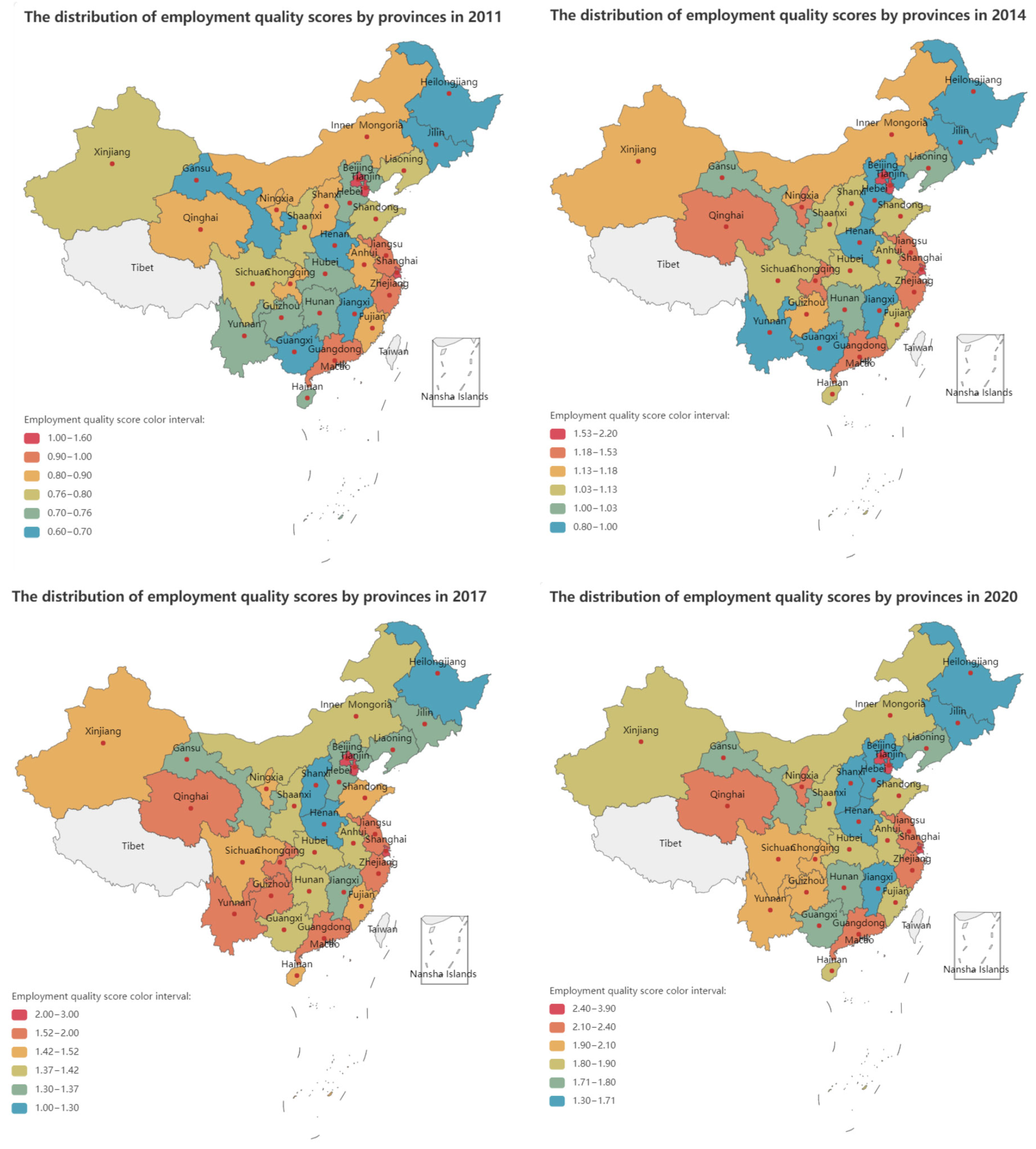
4.2.1. Expansion and Visualization in Spatial Dimension

According to the fiber operation of the tensor, fixing the time dimension and the index dimension, 10 × 18 tensor fibers along the space dimension could be obtained. Four of these fibers were taken as examples for visualization, and in order to more fully display the development of employment quality, the index dimension was fixed on the employment quality score comprehensive index, calculated by score coefficient Y. In the time dimension, the fibers were fixed in 2011, 2014, 2017, and 2020, respectively. Figure 1 shows these four sample fibers. After ranking according to the score of the comprehensive index of employment quality, the scores of the top regions greatly differed, and the scores of the middle and lower regions were more concentrated, so the legend in Figure 1 did not adopt the uniform partition method. As shown in Figure 1, with the implementation of the western development policy, the quality of employment in the western region was steadily improving, but the development potential of the quality of employment in central China was insufficient, and it was gradually being overtaken by the western region. The development span of the quality of employment in various provinces showed a trend of increasing, and the development of the quality of employment showed a significant unbalanced trend, which needed to be improved.

4.2.2. Expansion and Visualization in Time and Space Dimensions

According to the slicing operation of the tensor and the fixed index dimension, 18 slices of the tensor along the space and time dimensions could be obtained. In order to show the comprehensive situation of the development of employment quality, the slices were fixed on the comprehensive index of employment quality Y for visualization. The overall trend of the employment quality situation over time and region can be seen from Figure 2. From the perspective of the whole country, the average employment quality of China from 2011 to 2020 fluctuated around 1.3795, and the overall level of employment quality was not high, but it was showing an overall linear upward trend, indicating that our employment quality was developing healthily and improving steadily. From a provincial perspective, Beijing, Shanghai, and Tianjin scored the highest in employment quality, followed by Zhejiang, Guangdong, and Jiangsu. Jiangxi, Heilongjiang, and Henan scored the lowest. From the perspective of the situation of various provinces, in the past 10 years, the employment quality scores of Beijing and Shanghai have grown rapidly, firmly ranking in the top two, and their advantages have become increasingly obvious. Tianjin’s employment quality score ranked third, but the gap between it and the top two gradually widened, and the gap between it and the following provinces gradually narrowed.

From 2011 to 2020, Guizhou, Sichuan, Yunnan, Guangxi, and Gansu provinces had a rapid increase in employment quality. These five provinces are all from the western region of China, indicating that the strategy of large-scale development of the western region was effective and the employment quality in the western region was steadily improving. The employment quality in Inner Mongolia, Anhui, Liaoning, Shanxi, Hebei, and Henan rapidly declined. These six provinces are all from the central and eastern regions. Although the quality of employment in the six provinces was also steadily increasing, the increase was small, and the growth was relatively slow.

It is worth noting that Sichuan Province has a strong radiation effect on the development of employment quality in neighboring provinces. It became the core of driving the growth of surrounding employment quality between 2011 and 2020. As can be seen from Figure 3, Sichuan’s neighboring provinces have all developed rapidly in employment quality, driven by Sichuan. After Sichuan Province completed the post-disaster reconstruction work of the Wenchuan Earthquake in 2011, its economy developed rapidly, and it has become the province with the fastest economic growth in recent years. While Sichuan is comprehensively developing its own employment quality, it has also had a strong radiation effect on neighboring provinces, driving the rapid development of employment quality in the neighboring provinces of Guizhou, Yunnan, Guangxi, and Gansu. Beijing and Tianjin had a strong siphon effect on the development of employment quality in neighboring provinces. The employment quality of the provinces near Beijing and Tianjin showed a downward trend.

5. Spatial Econometric Analysis of Influencing Factors of Employment Quality in China’s Provinces

5.1. Spatial Correlation Analysis of Employment Quality in China’s Provinces

Through exploratory spatial data analysis, the spatial correlation of China’s inter-provincial employment quality was studied. As can be seen from

Table 4. Moran’s I test of employment quality.

Year	Moran’s I	E (I)	Sd	Z (I)	p-Value
2011	0.2538	−0.0357	0.1045	2.7367	0.013
2012	0.2495	−0.0357	0.1109	2.4696	0.024
2013	0.2536	−0.0357	0.1108	2.5105	0.024
2014	0.2347	−0.0357	0.1103	2.3545	0.031
2015	0.2458	−0.0357	0.1110	2.4408	0.030
2016	0.2438	−0.0357	0.1117	2.4118	0.030
2017	0.2634	−0.0357	0.1114	2.5973	0.025
2018	0.2294	−0.0357	0.1108	2.3038	0.033
2019	0.2288	−0.0357	0.1101	2.3038	0.031
2020	0.2068	−0.0357	0.1108	2.0898	0.043

, the global Moran’s I index of employment quality scores of 30 provinces in China from 2011 to 2020 were all greater than zero, and the statistical test values were all less than 0.05, indicating that China’s inter-provincial employment quality presented significant spatial autocorrelation during the study period. Provinces with higher employment quality tend to be adjacent to provinces with higher employment quality in space, while provinces with lower employment quality tend to be adjacent to provinces with lower employment quality in space. Therefore, it is suitable for the spatial econometric analysis of the factors affecting the employment quality in China’s provinces.

5.2. Analysis of Influencing Factors of Employment Quality in China’s Provinces

Through spatial autocorrelation analysis, it was found that China’s inter-provincial employment quality has spatial correlation. Therefore, a spatial econometric model can be built to explore the impact of various influencing factors on China’s inter-provincial employment quality.

5.2.1. Selection of Variables and Data Test

According to the principles of representativeness and availability, relevant explanatory variables were selected based on the existing research and the actual situation of each region. The explained variable was the employment quality score, and the explanatory variables were industrial structure, urbanization level, industrialization level, investment policy, foreign trade dependence, informatization level, price level, fiscal expenditure, and technology level. It should be noted that due to the broad concept of the informatization level, the informatization level defined in this study refers to the ability and level of a country or region in the application of information technology, covering information infrastructure construction, technology research and development, resource development and utilization, technology application, as well as information industry development. Improving the informatization level helps to promote economic development and social progress, improve production efficiency and quality of life, and promote industrial transformation, upgrading, and innovation development. This article used the ratio of the number of employees in the post and telecommunications industry in each province to the total population in each province, divided by the ratio of the number of employees in the post and telecommunications industry nationwide to the total population nationwide, to measure the informatization level. As the fundamental purpose of the analysis of employment quality was to improve the employment imbalance, economic development had a stronger and more significant impact on employment quality, so more emphasis was placed on the consideration of variables related to economic factors, as shown in

Table 5. Index system of the influencing factors of employment quality.

Sort	Index Name	Abbreviation	Index Interpretation
Explained variable	Employment quality	EQ	Employment quality score
Explanatory variable	Industrial structure	IS	Value added of the primary industry + value added of the secondary industry × 2 + value added of the tertiary industry × 3
	Urbanization level	URBAN	Proportion of urban population in total permanent population
	Industrialization level	IL	Per capita industrial output
	Investment policy	IP	Per capita fixed asset investment
	Dependence on foreign trade	DFT	Degree of dependence on imports and exports
	Informatization level	IT	(Number of post and telecommunications employees in each province/total population in each province)/(Number of post and telecommunications employees in the country/total population in the country)
	Price level	PR	Consumer price index
	Fiscal expenditure	FIS	Fiscal expenditure
	Technical level	TFP	Total factor productivity

.

The ADF–Fisher test method was used to conduct unit sum test on the variables used in the study. The stationarity test results showed that variables EQ, IS, IP, DFT, IT, FIS, and TFP were zero-order unstable, and all variables showed stationarity results at the first- and second-order levels, indicating that the test variables had first-order stationarity. The results obtained from this set of data have scientific significance. In order to avoid the interference of heteroscedasticity on the empirical results, a regression analysis was carried out on the logarithm of the original data.

5.2.2. Regression Results of Spatial Durbin Model

The Lagrange multiplier test (LM test) and its robust test results showed that the LM test corresponding to SLM and the robust test both passed the 1% significance level test, and the LM test corresponding to the spatial error panel model SEM also passed the 1% significance level test. The robust test corresponding to SEM passed the 1% significance level test, indicating that SLM is superior to SEM, and the test results of SLM and SEM were both significant, so it was necessary to further select the SDM model for estimation and comparison. SDM regression results showed (

Table 6. SDM regression results of influencing factors of employment quality in China.

Variable	No Fixed Effect	Spatial Fixed Effect	Time Fixed Effect	Double-Fixed Effect in Space and Time
IS	4.0537 ***	1.0572 **	4.1263 ***	−0.6689 *
URBAN	0.4379 ***	−2.0799 ***	0.1446	−2.3412 ***
IL	−0.0234	−0.0275	0.0441	0.0755 *
IP	−0.0900 **	−0.0049	−0.0916 **	0.0624 **
DFT	−0.0814 ***	−0.1537 ***	−0.0544 ***	−0.1348 ***
IT	0.2002 ***	0.0644 **	0.2240 ***	0.0210
Price	0.6172	−1.7536 *	−0.4606	−1.0051
Fiscal	0.0241	0.8284 ***	0.0110	0.1624 **
TFP	0.1563	−0.1060 *	0.0785	−0.1035 **
W * IS	2.8661 ***	−1.8073 **	4.6846 ***	−2.4773 ***
W * URBAN	−0.5106 **	2.6290 ***	−1.2731 ***	1.2748 ***
W * IL	−0.0699	0.1505	0.2021 **	0.2984 ***
W * IP	0.1576 **	−0.2018 ***	0.0151	−0.0861 *
W * DFT	0.0422	0.1711 ***	0.0537 *	0.0966 ***
W * IT	−0.1672 **	0.1100 *	−0.0049	0.1473 ***
W * Price	−0.3925 *	2.8501 ***	0.1003	−0.0551
W * Fiscal	0.0753	−0.1922	0.0388	−0.3583 ***
W * TFP	0.2666	0.0878	−0.1424	−0.1311
W * dep.var.	0.4680 ***	0.6090 ***	0.1670 **	0.3000 ***
intercept	−6.9725
R2	0.8968	0.9761	0.9098	0.9862
sigma2	0.0263	0.0068	0.0237	0.0035
log-likelihood	112.0350	323.6626	127.5496	401.9792

Note: *, **, and ***, respectively, indicate that the variable is significant at the levels of 10%, 5%, and 1%.

) that the R² values of four SDM effects were 0.8968, 0.9761, 0.9098, and 0.9862, respectively, with the Log-likelihood being 112.0350, 323.6626, 127.5496, and 401.9792, respectively. The error term squared (sigma²) and Log-likelihood values indicated that spatial fixed effects and spatial–time double-fixed effects were better estimated. From the significance level of the regression results of SDM, the spatial–time double-fixed effect was more significant than the estimation result of the spatial fixed effect. Therefore, we selected the spatial–time double-fixed effect in SDM to analyze the influencing factors of employment quality. The Wald and likelihood ratio (LR test) tests of SDM under spatial–temporal dual-fixed effects showed that: The Wald and LR test values of SLM were 93.8198 and 37.9455, and their adjoint probability values were 3.33 × 10⁻¹⁶ and 1.78 × 10⁻⁵, respectively. The Wald and LR test values of SEM were 26.8987 and 1.9489, respectively. The adjoint probability values were 2.75 × 10⁻¹⁴ and 2.00 × 10⁻³, respectively, both of which passed the test at the significance level of 1%, indicating that the model did not degenerate into SLM and SEM.

5.2.3. Decomposition of Spatial Effects of Factors Affecting Employment Quality in China’s Provinces

The spatial–temporal dual-fixed effect of SDM was selected to conduct a spatial econometric analysis on the quality of inter-provincial employment in China and its influencing factors from 2011 to 2020 (Table 6). In the table, the estimated coefficients of W * URBAN, W * IL, W * DFT, and W * IT are all positive, and all are significant at the 1% level, which indicates that the spatial spillover effects of urbanization level, industrialization level, foreign trade dependence, and informatization level on the surrounding provinces were positive. The estimated coefficients of W * IS, W * IP, and W * Fiscal in the table are negative and all are significant at 1%, which indicates that the spatial spillover effects of industrial structure, investment policy, and fiscal expenditure on the surrounding provinces were negative. Due to the spatial lag term, the estimated results of SDM cannot represent the marginal effects of the influencing factors, and the interpretation of the regression coefficient on the employment quality is not scientific. Further analysis of the direct effects, indirect effects, and total effects of the influencing factors is needed.

The direct effect represents the influence of various factors affecting employment quality on the employment quality of the province. From the direct effect, it can be seen that the industrial structure, urbanization level, industrialization level, investment policy, foreign trade dependence, informatization level, and technology level of each province had different degrees of influence on the employment quality of each province in China, and the significance level and effect strength of each variable were also different (

Table 7. Decomposition of the spatial spillover effect of the SDM model.

Variable	Direct Effect	Indirect Effect	Total Effect
IS	−0.8691 **	−3.6113 ***	−4.4804 ***
UR	−2.3028 ***	0.7738 **	−1.5290 ***
IL	0.1001 **	0.4403 ***	0.5404 ***
IP	0.0564 **	−0.0938 *	−0.0374 *
DFT	−0.1304 ***	0.0747	−0.0557 *
IT	0.0326 *	0.2093 ***	0.2420 ***
PR	−1.0258	−0.5375	−1.5633
FIS	0.1360	−0.4293 **	−0.2934 *
DFP	−0.1147 **	−0.2270 *	−0.3418 **

Note: *, **, and ***, respectively, indicate that the variable is significant at the levels of 10%, 5%, and 1%.

). (1) The Industrialization level, investment policy, and informatization level had promoting effects on employment quality, and the industrialization level had the largest effect coefficient (0.1001) on urban development quality, followed by investment policy and informatization level. (2) The effect of price level and fiscal expenditure on employment quality was not significant. (3) It is worth noting that the urbanization level and industrial structure had a significant negative effect on the quality of inter-provincial employment in China.

The Indirect effect represents the influence of factors affecting the employment quality of neighboring provinces on the employment quality of the province. From the indirect effect, we can see that the industrial structure, industrialization level, and informatization level were significant at the level of 1%, the urbanization level and fiscal expenditure were significant at the level of 5%, and the investment policy and technology level were significant at the level of 10%; that is, the spatial spillover effect was significant. (1) The influence of industrial structure, investment policy, fiscal expenditure, and technology level on the employment quality of neighboring provinces was negative, and the change in investment policy will have a “siphon effect” on various labor resources in neighboring provinces. (2) The influence of foreign trade dependence and price level on the employment quality of neighboring provinces was not obvious; that is, the development of these aspects had no effective radiating effect on the employment quality of neighboring provinces. (3) It is worth noting that, similar to the direct effect, the industrial structure was a negative effect of spatial spillover.

The total effect is the comprehensive influence strength of the factors affecting the employment quality of each province on the employment quality of China’s provinces. From the total effect, it can be seen that the industrial structure, urbanization level, industrialization level, and informatization level passed the significance test of 1%, the technology level passed the significance test of 5%, and the investment policy, foreign trade dependence, and fiscal expenditure passed the significance test of 10%. (1) The effect coefficient of the industrialization level and informatization level was positive, indicating that through industrialization development and informatization level improvement, China’s employment quality will be improved accordingly. (2) The total effect of the industrial structure and urbanization level was negative, indicating that the industrial structure and urbanization level had no promoting effect on employment quality.

Comprehensive analysis showed that the industrial structure had a significant negative effect on employment quality under the three effect models. In 2011, employment in the primary industry accounted for 34.74 percent, and that in the tertiary industry for 35.68 percent. In 2020, employment in the primary industry accounted for 23.60 percent and that in the tertiary industry accounted for 47.70 percent. At present, the number of employment opportunities in China’s primary industry has decreased significantly, while the number of employment opportunities in the tertiary industry has grown rapidly. In the process of the development and change of industrial structure, the labor force of the primary industry is easily replaced by science and technology, so as to flow to the second and third industries. The traditional service industry absorbs a large number of labor transferred from the primary industry, resulting in the tertiary industry’s inability for high-quality develop. At the same time, the reform of the household registration system and land policy promoted the transfer of the labor force in the primary industry, but due to the constraints of their own skills and industry thresholds, there are still large mobility barriers between industries for the transfer of the labor force in the primary industry. Moreover, a large part of the transferred agricultural labor force flows into the traditional service industry, thus forming the “anti-efficiency allocation” of labor force factors and hindering the healthy development of economic growth and employment quality.

6. Conclusions and Policy Suggestions

6.1. Conclusions

(1)

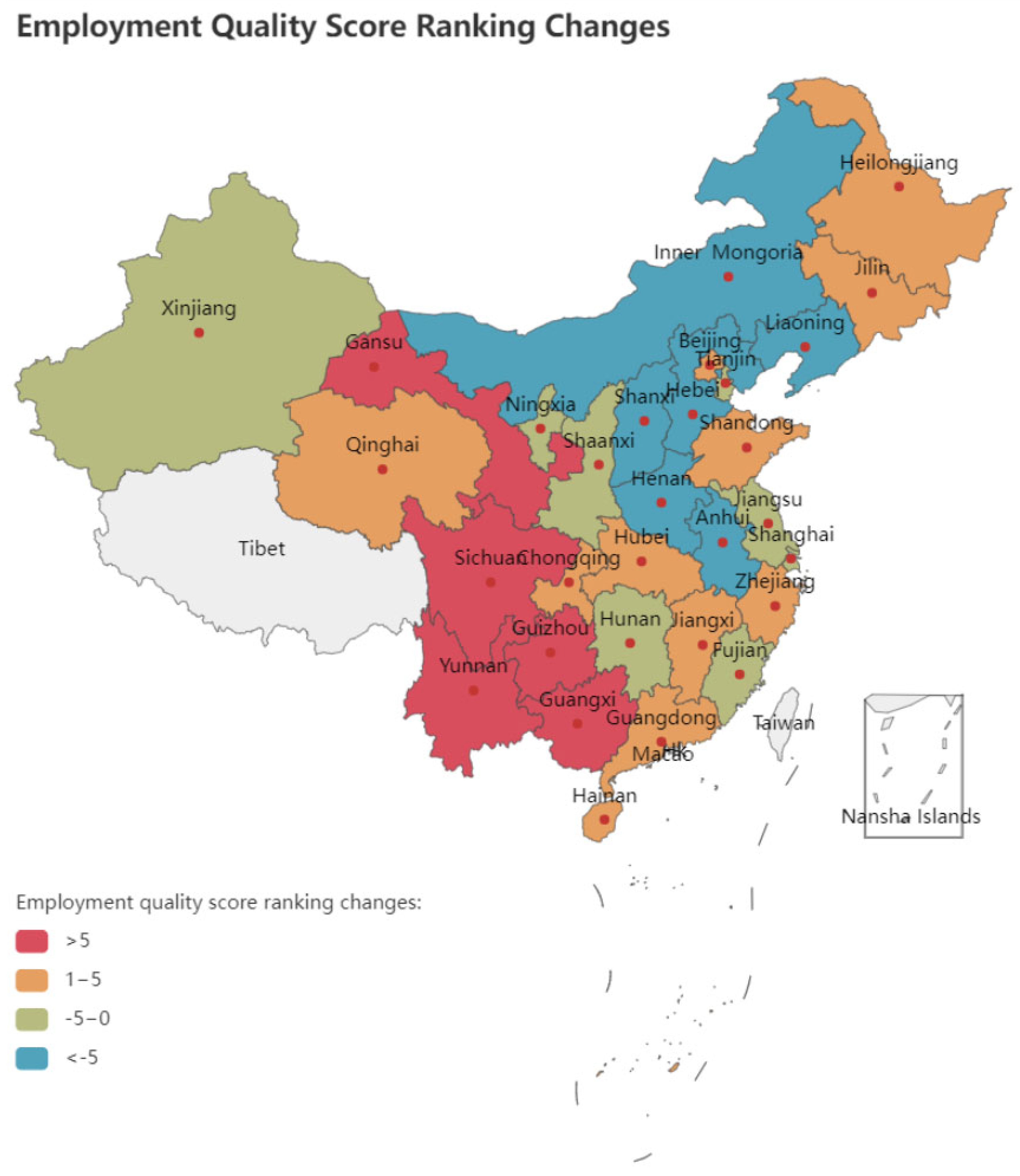
The overall level of employment quality in China was not high, the difference in employment quality between provinces was large, and the development gap in employment quality between provinces showed a trend of widening. Beijing, Shanghai, and Tianjin ranked as the top three in the overall score of employment quality, but the gap between Tianjin and Beijing and Shanghai was increasing, and the gap between Tianjin and the fourth place was gradually narrowing. Over the 10-year period, the provinces with the fastest growth in the overall score of employment quality were all from China’s western regions, while the provinces with the fastest lag were from central and eastern regions.

(2)

The development rate of employment quality in western China was fast, while the development of employment quality in central China was weak. Beijing and Shanghai, as China’s first-tier cities, have a strong momentum of development, with the fastest growth rate of employment quality among the 30 provinces, and their advantages are becoming more and more obvious. With the implementation of China’s western development policy, the quality of employment in the western region is steadily improving, but the quality of employment in central China shows insufficient development potential and has been gradually overtaken by the western region.

(3)

Sichuan has a strong radiating effect on the employment quality development of neighboring provinces, while Beijing and Tianjin have a strong siphon effect on the employment quality development of neighboring provinces. While the employment quality of Sichuan has developed rapidly, the employment quality of its neighboring provinces Guizhou, Yunnan, Guangxi, and Gansu has also developed rapidly. The employment quality of provinces near Beijing and Tianjin all showed a downward trend, and the decline rate was higher than 5 places.

(4)

The levels of industrialization and informatization promoted the development of employment quality in China’s provinces, while the industrial structure had a significant negative effect on the development of employment quality. Industrialization level, investment policy, and informatization level had significant positive effects on the employment in the province, and the industrialization level had the strongest effect. Urbanization level, industrialization level, and informatization level had significant positive effects on the employment of neighboring provinces, and the urbanization level had the strongest effect coefficient. The levels of industrialization and informatization had a significant positive effect on the employment quality of China’s provinces. The direct, indirect, and total effects of industrialization and informatization levels were significantly positive, indicating that they have a promoting effect on the development of employment quality in this province and neighboring provinces. It is worth noting that industrial structure and foreign trade dependence had significant negative effects in terms of direct effects, indirect effects, and total effects, especially the high negative effect coefficient of industrial structure, which has hindered the development of China’s employment quality. Industrial structure needs to be further optimized and upgraded, and high-quality development of industrial structure can promote high-quality development of employment quality.

6.2. Policy Suggestions

(1)

Strengthen inter-provincial cooperation and exchange: As the gap in the development of employment quality between provinces tends to widen, it is necessary to promote cooperation and exchange among provinces, share best practices, and jointly improve the quality of employment. Regular exchange meetings and cooperation platforms can be established among provinces to share best practices, experiences, and technologies. It is important to promote resource sharing among provinces in education and training, employment information, and other aspects to ensure that the labor force in each province can acquire the latest skills and knowledge. Encouraging project cooperation among provinces can help to jointly develop new employment opportunities and industries and promote the coordinated development of economy and employment.

(2)

Focus on supporting the central and western regions: The employment quality in western China has developed rapidly, and support for these regions should continue to be strengthened to further improve their employment quality. For central China, new growth points for improving employment quality need to be identified to ensure its sustainable development.

(3)

Exerting the radiation effect of Sichuan: Sichuan has a strong radiation effect on the development of employment quality in neighboring provinces and should further tap into and utilize this advantage to promote the improvement of employment quality in neighboring provinces. Optimizing the siphon effect of Beijing and Tianjin: Beijing and Tianjin have a strong siphon effect on the development of employment quality in neighboring provinces and should optimize their employment policies to ensure that while attracting talent, they also provide more employment opportunities and a better employment environment for the labor force in neighboring provinces.

(4)

Improve the levels of industrialization and informatization: The levels of industrialization and informatization have a positive impact on the improvement of the quality of employment in provincial areas. We should continue to promote the processes of industrialization and informatization to create conditions for the improvement of the quality of employment in provincial areas. Adjust the industrial structure: The industrial structure has a significant negative effect on the development of the quality of employment. We should adjust the industrial structure to promote its coordinated development with the quality of employment. For example, we should encourage the development of the tertiary industry, especially those industries that can provide more high-quality jobs.

This study aimed to enhance the employment quality in China. It examined and evaluated the current status and influencing factors of employment quality development. The primary contributions of this study were as follows: (1) In terms of measuring the employment quality index system, we employed principal tensor analysis, achieving dimension reduction while preserving the original structure of the data. (2) In analyzing the influencing factors of employment quality, we utilized spatial econometric models to investigate the mechanisms of influencing factors on employment quality from both spatial and temporal perspectives. However, there are still areas that require further improvement and in-depth research: (1) The development evaluation index of employment quality in this study was constructed based on a comprehensive consideration of the connotation of high-quality development and on scholars’ research. It was designed based on the availability and operability of data. Nevertheless, due to data limitations, qualitative indicators related to micro-workers are not yet included in the evaluation system. As the data continues to improve in the future, the development evaluation index system of employment quality should be further supplemented and refined. (2) This study primarily focused on the provincial level in China to explore the current status and influencing mechanisms, as well as spillover effects, of employment quality development. Future research could delve deeper into influencing factors at the city level and above.

References

1. Grossmann, V. Quality Improvements, the Structure of Employment, and the Skill-bias Hypothesis Revisited. Top. Macroecon. 2002, 2, 21–29. [Google Scholar] [CrossRef]
2. Arranz, J.M.; García-Serrano, C.; Hernanz, V. Employment Quality: Are There Differences by Types of Contract? Soc. Indic. Res. 2018, 137, 203–230. [Google Scholar] [CrossRef]
3. Chreneková, M.; Melichová, K.; Marišová, E.; Moroz, S. Informal Employment and Quality of Life in Rural Areas of Ukraine. Eur. Countrys. 2016, 8, 135–146. [Google Scholar] [CrossRef]
4. Cocks, E.; Thoresen, S.H.; Lee, E. Pathways to Employment and Quality of Life for Apprenticeship and Traineeship Graduates with Disabilities. Int. J. Disabil. Dev. Educ. 2015, 62, 131–136. [Google Scholar] [CrossRef]
5. Aerden, K.V.; Puig-Barrachina, V.; Bosmans, K.; Vanroelen, C. How Does Employment Quality Relate to Health and Job Satisfaction in Europe? A Typological Approach. Soc. Sci. Med. 2016, 158, 132–140. [Google Scholar] [CrossRef]
6. Ming, J.; Wang, M.L. Can Job Conversion Improve the Employment Quality of Migrant Workers? China Soft Sci. 2015, 4, 49–62. [Google Scholar] [CrossRef]
7. Li, N.; Xu, R.H. Research on statistical issues related to employment quality. Stat. Res. 2016, 33, 111–112. [Google Scholar] [CrossRef]
8. Mao, J.J.; Lu, L.; Shi, Q.H. Research on factors affecting the employment quality of migrant workers in Shanghai—Based on the perspective of intergenerational differences. China Soft Sci. 2020, 65–74. [Google Scholar] [CrossRef]
9. Ling, L. Employment quality and residents’ subjective welfare: An empirical study based on the survey of Labor dynamics in China. J. Stat. Res. 2002, 39, 149–160. [Google Scholar] [CrossRef]
10. Chen, G.S.; Ni, C.Y.; Zhang, H.Y. An empirical study on the relationship between human capital investment and rural non-agricultural employment: A case study of Hunan Province. Econ. Geogr. 2015, 35, 155–159. [Google Scholar] [CrossRef]
11. Yang, Y.L.; Zhai, C.Y. Measurement and correlation analysis of urbanization quality and employment quality in China. J. Northeast. Univ. (Soc. Sci. Ed.) 2016, 18, 42–48. [Google Scholar] [CrossRef]
12. Zheng, H.L.; Liu, Z.M.; Lu, L.L. The linkage analysis of employment structure, industrial structure and economic growth in Hebei Province. Areal Res. Dev. 2018, 37, 63–68. [Google Scholar] [CrossRef]
13. Ma, R.; Yin, L.S.; Nie, Y. Research on the induced effect of fiscal expenditure on spatial employment aggregation in Central China. Jianghuai Forum 2019, 60–65. [Google Scholar] [CrossRef]
14. Sheng, Y.N. Effects of birth policy adjustment on female employment quality. Popul. Econ. 2019, 62–76. [Google Scholar] [CrossRef]
15. Xie, M.M.; Xia, Y.; Pan, J.F.; Guo, J.F. Artificial Intelligence, technological progress and low-skill employment: An empirical study based on Chinese manufacturing enterprises. Chin. J. Manag. Sci. 2019, 28, 54–66. [Google Scholar] [CrossRef]
16. Zhou, C.; Shen, X.X. Research on the influence of government training on the employment quality of migrant workers. Math. Stat. Manag. 2021, 40, 692–704. [Google Scholar] [CrossRef]
17. Zhang, M.Z.; Yue, S. The impact of external tariff changes on regional labor employment in China. China Ind. Econ. 2022, 113–131. [Google Scholar] [CrossRef]
18. Leibovici, D.; Sabatier, R. A singular value decomposition of a k-way array for a principal component analysis of multiway data, PTA-K. Linear Algebra Its Appl. 1998, 269, 307–329. [Google Scholar] [CrossRef]
19. Gao, X.D.; Pan, Y.X.; Bo, Q.X. A spatial econometric analysis of the influencing factors of employment quality in China. Areal Res. Dev. 2022, 41, 13–18. [Google Scholar] [CrossRef]
Figure 1. Employment quality scores in 2011, 2014, 2017, and 2020.
Sustainability 16 01458 g001
Figure 2. Change trend of the employment quality score in time and region.
Sustainability 16 01458 g002
Figure 3. The change in employment quality score ranking from 2020 to 2011.
Sustainability 16 01458 g003