Can Green Finance Mitigate China’s Carbon Emissions and Air Pollution? An Analysis of Spatial Spillover and Mediation Pathways

Abstract

China faces a multi-objective environmental governance dilemma involving achieving fundamental ecological environment improvement, carbon peaking, and carbon neutrality. In this study, we constructed indicators of the level of green finance development through the entropy-weighted TOPSIS evaluation model, and adopted the two-way fixed-effect spatial Durbin model (SDM) and the multiple spatial mediation effect model to explore the impacts and paths of green finance as a policy tool to promote environmental sustainability in carbon emissions and environmental pollution using panel data from 30 provinces in China between 2007 and 2019. The research results show that green finance (GF) can significantly reduce carbon emission intensity (CEI) and air pollution (AP). Moreover, the role of GF in reducing AP becomes weaker due to increased levels of green finance in neighboring regions negatively affecting local air quality. Mediation path analysis shows that GF reduces CEI and AP mainly by promoting the optimization of energy structures and technological progress. The results of regional heterogeneity analysis show that there is variability in the pathway of the impact of GF on CEI and AP in different regions, and the Western region is more sensitive to GF policies. Therefore, policymakers should give their full attention to the functions of GF to mitigate China’s carbon emissions and environmental pollution.

1. Introduction

Climate change and air pollution (AP) are urgent issues in most countries [1,2]. As the world’s largest developing country, China’s manufacturing sector contributes significantly to economic development, and these major industries, such as thermal power, iron and steel, and cement, bring high levels of carbon emissions and air pollutants. Therefore, China faces serious air pollution and high carbon emission problems following 40 years of rapid economic growth [3,4]. Green finance (GF), which promotes economic transformation and sustainable social development oriented towards environmental protection, low-carbon development, and sustainable development [5], has been emphasized and supported by the Chinese government. The Chinese government has issued a series of normative and guidance documents to improve the green financial system, such as Opinions on the Implementation of Environmental Policies and Regulations (2007) and Guidelines for Establishing the Green Financial System (2016). Additionally, the Chinese government made commitments that China will strive to reach its carbon peak by 2030 and achieve carbon neutrality by 2060 at the 75th UN General Assembly in 2020. Green finance is strongly promoted and developed as it helps to facilitate the flow of funds to green industries and projects, promotes low-carbon and sustainable development, and plays an important role in achieving the dual carbon goals. China has gradually formed a multilevel green financial product and market system that includes green credit, bonds, insurance, funds, trusts, and carbon financial products.

In theory, GF can significantly reduce carbon emissions and AP. First, GF provides financial support for green projects, including forest and grassland carbon sinks, environmental infrastructure, pollution control, and biodiversity conservation [6]. Second, heavily polluting enterprises must carry out industrial upgrading and transformation owing to strict constraints on financing scales [7] and financing costs [8] caused by GF. Third, GF promotes renewable energy [9]. The consumption of fossil fuels, particularly coal, generates large amounts of carbon and pollutants, and replacing fossil fuels with renewable energy is very effective in reducing levels of carbon emissions and air pollutants. Finally, GF promotes technological progress through lower-cost finance. On the one hand, technological progress improves the efficiency of energy utilization and decreases energy intensity [10]. On the other hand, the development of technologies related to renewable energy, such as solar energy, wind energy, and energy storage technology [11], can reduce the cost of renewable energy utilization and the consumption of fossil energy.

In the related literature, GF, as a type of environmental supervision, has typical policy spillover effects. First, the development of GF provides companies with clear policy directions that high-emission enterprises will be restricted [12], which facilitates surrounding regional enterprises to undergo a green and low-carbon transition for long-term development. Second, the development of GF enhances public awareness of environmental protection [13], which continuously spreads to neighboring areas with population migration. Finally, the development of GF promotes green technological progress, which has a strong spillover effect [14]. Advances in technology that reduce carbon emissions and pollution will reduce the economic and legal risks that businesses are exposed to due to environmental protection issues. Once an enterprise adopts an advanced green process or technology, surrounding enterprises will compete to adopt it as soon as possible.

For a long period, the development of GF in China has been highly unbalanced. China’s economic development is characterized by significant disparities between regions, with the Eastern coastal region having a high level of economic development and a well-developed financial industry. As the economy grows, people focus on environmental protection and are eager to improve environmental quality [15], and GF is usually at a high level. The Western region is sparsely populated and rich in natural resources but lacks economic development. Rich natural resources attract continued relocation of energy-intensive enterprises, generating large amounts of carbon emissions and pollution. However, local governments have been unable to formulate strict environmental regulations to restrict these high-emission enterprises because of raising income levels and developing the economy they bring. Consequently, GF in these areas is at a low level. Against this background, can GF promote reductions in AP and carbon emissions? How does GF affect AP and carbon emissions? How does GF affect AP and carbon emissions in different regions of China? These questions require further investigation.

To address these issues, we constructed a GF development level index and carried out an in-depth analysis using a spatial econometric model with panel data from 30 Chinese provinces from 2007 to 2019. The main contributions of this study are as follows: First, we built indicators to measure the development level of GF through the entropy-weighted TOPSIS method from the three aspects of green credit, green investment, and green support, which is a more comprehensive approach compared to those of some studies that use green credit to indicate the level of green finance development [16], and is a useful supplement to the existing research. Second, after providing an overview and summary of the existing literature, we explored the mechanisms and effects of GF on carbon emissions and AP by region and from multiple perspectives to provide references and support for green development practices in countries where there are regional differences in the development of green finance, such as China.

The remainder of this study is organized as follows. Section 2 reviews the relevant literature. Section 3 describes the research methods and data. Section 4 presents our empirical results. The final section summarizes the conclusions and provides the policy implications.

2. Literature Review

2.1. Impact of GF

Most studies have explored the impact of GF on environmental protection, low-carbon economic transformation, and sustainable development. Green finance mainly promotes the development of green industries, reduces carbon emissions, and lowers environmental risks by promoting green technological innovation and improving corporate performance [17]. However, some studies have shown that the development and effectiveness of green finance has been limited due to the high cost of climate investments [18], poor green project selection and management, risk–return trade-offs, and a lack of analytical tools and expertise for identifying and evaluating green project risks [19].

2.2. Impact of GF on Carbon Emissions and Pollution

Regarding the impact of GF on carbon emissions, some scholars believe that GF can effectively promote the reduction of carbon emissions [20]. Still, other scholars have found, through empirical analysis, that the carbon reduction effect of GF is not always effective. For example, Zhang et al. [21] showed that the carbon emission reduction efficiency of GF is not obvious in the Western region of China. In addition, the emission reduction efficiency of GF is affected by factors such as insufficient private investment in green funds [22] and difficulties in environmental information disclosure [23], leading to an insignificant carbon reduction effect.

Regarding the impact of GF on pollutant emissions, most studies show that GF can reduce pollutant emissions, but these related studies are still controversial. For example, Lan et al. [24] showed that the relationship of GF and pollutant emissions is characterized by a non-linear “inverted N”, and the development of GF does not always promote pollution reduction. Zhang et al. [25] found that in economically developed regions the pollutant emission reduction effect of green financial policy is weaker than that in less developed regions.

2.3. Mechanism of GF’s Effects on Carbon Emissions and Pollution

Existing studies on the mechanism of GF’s effects on pollution and carbon emissions can be summarized based on three aspects: economic scale, economic structure, and technological innovation. Considering the economic scale, GF promotes the transition of the economy in a green and low-carbon direction, which has a positive effect on environmental improvement [26]. In contrast, the expansion of the scale of production generated by the development of finance can exacerbate environmental pollution and carbon emissions in some countries and regions [27]. The economic structure is usually studied in terms of both ES and IS. For example, Xu et al. [28] studied the GF reform and innovation pilot zone in China and found that GF improved air quality by promoting IS optimization. Xiang et al. [29] constructed a panel threshold model with IS and ES as the threshold variables, finding that the inhibitory effect of GF on AP through IS optimization is greater than that through ES optimization. With the optimization of IS and the improvement of clean energy efficiency, the influence is gradually weakened, which was shown as a non-linear relationship. Huang et al. [20] found that GF through IS and ES reduces carbon emission intensity. Based on the Hansen threshold regression model, Bai et al. [30] proved that the relationship between green financial development and carbon emissions is one of the inverted N-type with IS as the threshold, and the impact of GF on carbon emissions in the Central region is characterized by an inverted U-type relationship. Regarding technological innovation, studies have shown that GF eases enterprises’ financial constraints in favor of green technological innovation and promotes carbon dioxide emission and AP reduction [31].

Based on the above analysis, most of the literature shows that GF affects pollution and carbon reduction. Still, this effect is not significant in some regions [21] and is non-linear in some situations [24]. It is therefore necessary to carry out studies regarding the effects of GF on AP and carbon emissions, taking into consideration regional heterogeneity in China. Furthermore, there are many studies on the mechanism of GF’s effects on the reduction of carbon emissions and pollution, with this impact not a simple enhancement or inhibition but rather characterized by a complex non-linear relationship. As there is no consensus regarding the mechanism by which GF affects AP and carbon emissions, further studies are warranted.

3. Methodology and Data

The purpose of our study was to investigate the impact of GF on CEI and AP. The development of GF is mainly driven by policies, and the scope of action of these green finance-related policies issued by the Chinese government is generally mainland China; thus, Hong Kong, Macao, and Taiwan are outside the scope of our study. Furthermore, Tibet was excluded from the sample due to missing data. In addition, we assume that Hainan’s neighbor is Guangdong and vice versa to ensure that each province has neighbors for the spatial econometric analysis [32]. Eventually, data relating to 30 provinces in China, excluding Hong Kong, Macao, Taiwan, and Tibet, from 2007 to 2019 were selected as the research sample. Then, we constructed the benchmark model, the spatial econometric model, and the spatial mediation effect model to analyze the spatial spillover and mediation pathways of GF; the data and process framework of the methodology are shown in Figure 1.

3.1. Variables and Data

3.1.1. Green Finance (GF) Development Index

GF generally includes multiple dimensions, such as green credit, bonds, investments, funds, insurance, and green support, which makes it difficult to comprehensively measure the development level of GF. Most of the literature usually uses green credit as an approximate substitute for green finance [33,34]. With the development of green finance, green investment and green support are taking an increasingly important place in the green financial system [35], and the development of green credit is not sufficient to indicate the level of development of green finance. Therefore, in this study we used three datasets—green credit, green investment, and green support—to measure the level of green financial development in the region; the data were derived from the China Industrial Statistics Yearbook and the China Statistical Yearbook (details are shown in the Supporting Information, S2.2). To ensure the objectivity and validity of the indicators for measuring the development level of GF, we adopted the entropy weight Technique for Order Performance by Similarity to an Ideal Solution (TOPSIS) [36] method to construct a green finance development index and used the Criteria Importance Through Intercriteria Correlation (CRITIC) [37] weighting method to recalculate the green finance development index for the robustness test (described in the Supporting Information, S1).

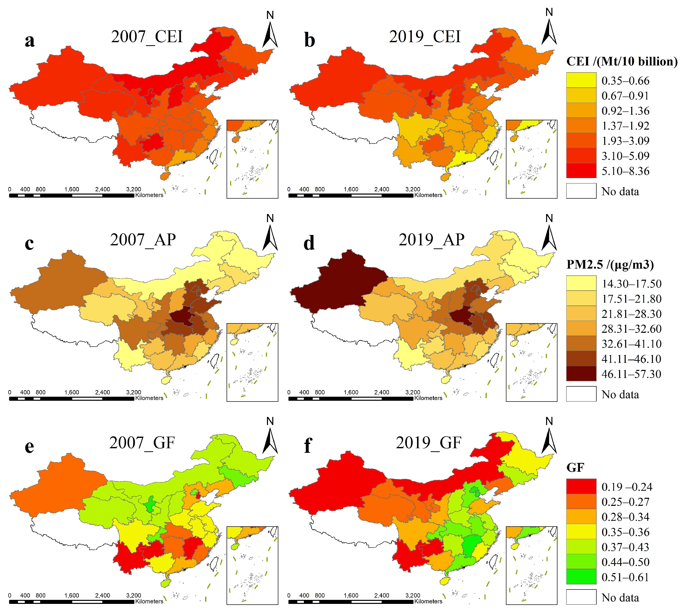
3.1.2. Carbon Emission Intensity (CEI) and Air Pollution (AP)

In this study, carbon emission intensity (CEI) and PM_2.5 were chosen to represent carbon emissions and air pollution (AP), respectively, and the data were derived from the Carbon Emission Accounts & Datasets (CEADs) and the Atmospheric Composition Analysis Group of Washington University (details are described in the Supporting Information, S2.1). CEI is sufficient and meaningful for denoting carbon emissions because it has been an important focus of the Chinese government’s efforts to control carbon emissions since the first comprehensive policy document to address climate change, the China National Climate Change Program, was issued by the Chinese government in 2007. Particulate Matter 2.5 (PM_2.5) is an air pollutant produced as a result of human industrial activity and poses a serious risk to public health and environmental quality. In the Air Pollution Prevention and Control Action Plan issued by the Chinese government in 2013, the reduction of PM_2.5 concentration was regarded as one of the goals towards achieving AP control, which is the reason why this paper takes PM_2.5 concentration as a variable to characterize AP.

Below, we illustrate the spatial distribution of CEI, AP, and GF in the 30 provinces of China in 2007 and 2019 (shown in Figure 2); the ranges of values of CEI and AP are 0.35–8.36 Mt/10 billion and 14.3–57.3 μg/m³, respectively. Figure 2 represents obvious spatial agglomeration of CEI, AP, and GF. We used Moran’s I to test the overall spatial autocorrelation—the details of this are described in the Supporting Information, S3. All the results of Moran’s I were significantly positive at the 1% level, indicating that GF, CEI, and AP have a positive spatial autocorrelation, which means the spatial econometric model is the best choice for analyzing the impact of GF on CEI and AP.

3.1.3. Other Control Variables

According to the research of Nie et al., environmental regulation can improve the environmental quality of regions by prompting the transfer of high-emission and high-pollution enterprises, accompanied by the optimization of the local energy consumption structure and the transformation and upgrading of the local IS [38]. Nevertheless, environmental regulation can promote innovation in green technology, thus improving the quality of the local environment [39]. Combined with the previous literature review, we selected ES, IS, and technology (T) as mediation variables to explore the mediation pathways of GF in reducing CEI and AP. Additionally, some studies have shown that urbanization (U) [27], foreign direct investment (FDI) [40], global openness (OP) [41], market maturity (MAR) [42], and level of economic development (PGDP) [43] affect CEI and AP. We also controlled these variables to ensure the reliability of the research results. The data were derived from the National Bureau of Statistics of China (NBS), the Wind database, and the relevant statistical yearbooks (details are shown in the Supporting Information, S2); the descriptive statistics are shown in

Table 1. Descriptive statistics of relevant variables.

Abbreviation	Variables	N	Means	Std. Dev.	Min	Max
CEI	Carbon emission intensity	390	2.527	1.661	0.347	10.21
AP	Air pollution	390	46.78	17.61	14.3	91.2
GF	Green finance development index	390	0.374	0.0863	0.191	0.79
IS	Industrial structure	390	120.4	67.41	52.71	523.4
ES	Energy structure	390	66.52	18.55	2.263	96.12
T	Technology	390	0.169	0.139	0.0204	0.732
U	Urbanization	390	55.26	13.41	28.25	94.15
MAR	Market maturity	390	26.08	12.48	3.006	56.96
FDI	Foreign direct investment	390	2.335	2.064	0.0107	12.1
OP	Openness	390	15.35	16.48	0.688	88.45
PGDP	Economic development level	390	38,020	21,835	7778	128,425

Note: N, Means, Min., and Max. are the number of objects, average values, minimum values, and maximum values, respectively; Std. Dev. refers to the standard deviations.

.

3.2. Research Methodology

3.2.1. Benchmark Model

Before analyzing the spillover effects of GF, we constructed a two-way fixed-effects model as a benchmark model to preliminarily analyze the impact of GF on CEI and AP, and the variables were logarithmically transformed to eliminate possible heteroscedasticity issues. This model is shown in Equation (1):

$$\begin{array}{l}{lnY}_{it}={\alpha }_0+{\alpha }_1{lnGF}_{it}+{\alpha }_2{lnIS}_{it}+{\alpha }_3{lnES}_{it}+{\alpha }_4{lnT}_{it}+{\alpha }_5{lnU}_{it}+{{\alpha }_{6}lnFDI}_{it}+{\alpha }_7{lnOP}_{it}+{\alpha }_8{lnMAR}_{it}\\ \hspace{1em}\hspace{1em}\hspace{1em}\hspace{1em}\hspace{1em}\hspace{1em}\hspace{1em}+{\alpha }_9{lnPGDP}_{it}+{\nu }_i+{\mu }_t+{\epsilon }_{it}\end{array}$$

(1)

where the subscript $i$ denotes the region, $t$ is the year, $Y_{it}$ is the dependent variable, which in this study refers to the carbon emission intensity ${CEI}_{it}$ and air pollution ${AP}_{it}$. ${GF}_{it}$ is the core explanatory variable for GF. Moreover, ${IS}_{it}$, ${ES}_{it}$, $T_{it}$, $U_{it}$, ${FDI}_{it}$, ${OP}_{it}$, ${MAR}_{it}$, and ${PGDP}_{it}$ as control variables represent IS, ES, technology level, urbanization level, foreign direct investment, openness, market maturity, and economic development level, respectively. ${\nu }_i$ is the individual fixed-effect, ${\mu }_t$ is the time fixed-effect, and ${\epsilon }_{it}$ is a random disturbance term.

3.2.2. Spatial Econometric Model

The spatial weight matrix must be defined before constructing the spatial econometric model. Two types of spatial weight matrices were used in this study: the geographical contiguity spatial weight matrix (W1) and the economic distance spatial weight matrix (W2) (described in the Supporting Information, S4). Furthermore, to explore the spatial effects of GF on CEI and AP, spatial spillovers measured by the spatial lags of the dependent and independent variables were incorporated, and spatial econometric models were constructed based on the benchmark model mentioned above. In general, three models have been widely applied in empirical spatial analysis studies: the spatial autoregressive model (SAR), the spatial error model (SEM), and the SDM; we performed model testing to select the appropriate model. We conducted the LR, Hausman, and Wald tests based on the spatial weight matrix W1, and the results show that the final spatial econometric model used in this study was the two-way fixed-effects SDM. We detail these approaches in the Supporting Information, S5. The model is shown in Equation (2).

$$\begin{array}{l}{lnY}_{it}={\alpha }_0+\rho W{lnY}_{it}+{\alpha }_1{lnGF}_{it}+{\alpha }_2{lnIS}_{it}+{\alpha }_3{lnES}_{it}+{\alpha }_4{lnT}_{it}+{\alpha }_5{lnU}_{it}+{{\alpha }_{6}lnFDI}_{it}+{\alpha }_7{lnOP}_{it}\\ \hspace{1em}\hspace{1em}\hspace{1em}\hspace{1em}\hspace{1em}\hspace{1em}\hspace{1em}+{\alpha }_8{lnMAR}_{it}+{\alpha }_9{lnPGDP}_{it}+{\gamma }_{1}W{lnGF}_{it}+{\gamma }_{2}W{lnIS}_{it}+{\gamma }_{3}W{lnES}_{it}+{\gamma }_{4}W{lnT}_{it}+{\gamma }_{5}W{lnU}_{it}\\ \hspace{1em}\hspace{1em}\hspace{1em}\hspace{1em}\hspace{1em}\hspace{1em}\hspace{1em}+{{\gamma }_{6}WlnFDI}_{it}+{\gamma }_{7}W{lnOP}_{it}+{\gamma }_{8}W{lnMAR}_{it}+{\gamma }_{9}W{lnPGDP}_{it}+{\nu }_i+{\mu }_t+{\epsilon }_{it}\end{array}$$

(2)

where W represents the spatial weight matrix, and the remaining variables are interpreted in the same manner as in Equation (1).

3.2.3. Spatial Mediation Effects Model

We construct a spatial mediating effect model to study the impact mechanism of GF on CEI and AP; the three-step calculation formulas of the multiple mediation effect model are shown in Equations (3)–(5).

$$\begin{array}{l}{lnY}_{it}={\alpha }_0+\rho W{lnY}_{it}+{\alpha }_1{lnGF}_{it}+{\alpha }_2{lnU}_{it}+{{\alpha }_{3}lnFDI}_{it}+{\alpha }_4{lnOP}_{it}+{\alpha }_5{lnMAR}_{it}+{\alpha }_6{lnPGDP}_{it}+{\gamma }_{1}W{lnGF}_{it}\\ \hspace{1em}\hspace{1em}\hspace{1em}\hspace{1em}\hspace{1em}\hspace{1em}\hspace{1em}+{\gamma }_{2}W{lnU}_{it}+{{\gamma }_{3}WlnFDI}_{it}+{\gamma }_{4}W{lnOP}_{it}+{\gamma }_{5}W{lnMAR}_{it}+{\gamma }_{6}W{lnPGDP}_{it}+{\nu }_i+{\mu }_t+{\epsilon }_{it}\end{array}$$

(3)

$$\begin{array}{l}{lnM}_{it}={\alpha }_0+\rho W{lnM}_{it}+{\alpha }_1{lnGF}_{it}+{\alpha }_2{lnU}_{it}+{{\alpha }_{3}lnFDI}_{it}+{\alpha }_4{lnOP}_{it}+{\alpha }_5{lnMAR}_{it}+{\alpha }_6{lnPGDP}_{it}\\ \hspace{1em}\hspace{1em}\hspace{1em}\hspace{1em}\hspace{1em}\hspace{1em}\hspace{1em}+{\gamma }_{2}W{lnGF}_{it}+{\gamma }_{3}W{lnU}_{it}+{{\gamma }_{4}WlnFDI}_{it}+{\gamma }_{5}W{lnOP}_{it}+{\gamma }_{6}W{lnMAR}_{it}+{\gamma }_{7}W{lnPGDP}_{it}+{\nu }_i\\ \hspace{1em}\hspace{1em}\hspace{1em}\hspace{1em}\hspace{1em}\hspace{1em}\hspace{1em}+{\mu }_t+{\epsilon }_{it}\end{array}$$

(4)

$$\begin{array}{l}{lnY}_{it}={\alpha }_0+\rho W{lnY}_{it}+{\alpha }_1{lnGF}_{it}+{{\alpha }_{2}lnM}_{it}+{\alpha }_3{lnU}_{it}+{{\alpha }_{4}lnFDI}_{it}+{\alpha }_5{lnOP}_{it}+{\alpha }_6{lnMAR}_{it}+{\alpha }_7{lnPGDP}_{it}\\ \hspace{1em}\hspace{1em}\hspace{1em}\hspace{1em}\hspace{1em}\hspace{1em}\hspace{1em}+{\gamma }_{1}W{lnGF}_{it}+{\gamma }_{2}W{lnM}_{it}+{\gamma }_{3}W{lnU}_{it}+{{\gamma }_{4}WlnFDI}_{it}+{\gamma }_{5}W{lnOP}_{it}+{\gamma }_{6}W{lnMAR}_{it}\\ \hspace{1em}\hspace{1em}\hspace{1em}\hspace{1em}\hspace{1em}\hspace{1em}\hspace{1em}+{\gamma }_{7}W{lnPGDP}_{it}+{\nu }_i+{\mu }_t+{\epsilon }_{it}\end{array}$$

(5)

where ${lnM}_{it}$ represents the mediator variables, which refer to technology ${lnT}_{it}$, industrial structure ${lnIS}_{it}$, and energy structure ${lnES}_{it}$, and the remaining variables are interpreted in the same way as in Equation (1).

The multiple mediation effect model is shown in Figure 3. First, it is a prerequisite for the analysis of the mediation effect model that the coefficient of GF in Equation (3) is significant, which represents the total effect of GF on CEI and AP. The second step simultaneously regresses Equations (4) and (5). If both the coefficient of GF in Equation (4) and the coefficient of mediator variables in Equation (5) are significantly not zero, it means that the mediation effects of mediator variables exist and the mediation effect is expressed by the product of the two. If the coefficient of GF in Equation (5) is significantly not zero, the mediator variable has a partial mediation effect. Otherwise, the mediator variables assume a complete mediating role in the impact of GF on CEI and AP. Because three mediator variables are used in this model, there are theoretically no complete mediation effects.

4. Empirical Results and Discussion

4.1. The Impact of GF on CEI and AP

4.1.1. Results of Non-Spatial Model

Table 2. Regression results from the non-spatial model.

	(1)	(2)	(3)	(4)	(5)	(6)
Variables	lnCEI	lnAP	lnCEI	lnAP	lnCEI	lnAP
lnGF	−0.1978 ***	−0.1682 ***	−0.1882 ***	−0.1810 ***	−0.1010 ***	−0.1338 ***
	(−5.44)	(−4.59)	(−5.16)	(−5.00)	(−2.88)	(−3.52)
Mediation variables	No	No	No	No	Yes	Yes
Other control variables	No	No	Yes	Yes	Yes	Yes
Individual FE	Yes	Yes	Yes	Yes	Yes	Yes
Time FE	Yes	Yes	Yes	Yes	Yes	Yes
Observations	390	390	390	390	390	390
R-squared	0.802	0.721	0.827	0.763	0.861	0.773

Note: Values in parentheses are t values. *** means p < 0.01. Mediation variables refer to lnES, lnT, and lnIS. Other control variables refer to lnU, lnMAR, lnFDI, lnOP, and lnPGDP. Columns (1) and (2) show the regression results of GF on CEI and AP when only GF is the control variable, while columns (3) and (4) show the regression results of GF on CEI and AP when the control variables are added, and columns (5) and (6) show the regression results of GF on CEI and AP when all the variables are controlled.

shows the regression results of the two-way fixed-effects benchmark model. As can be seen from the table, columns (1), (3), and (5) show that the impact of GF on CEI is significantly negative at 1%, and columns (2), (4), and (6) show that the impact of GF on AP is also significantly negative at 1%. This finding demonstrates that green financing significantly reduces CEI and AP. The coefficients of lnGF increase when we take a stepwise forward approach by adding control variables one by one. This suggests that the choice of variables is becoming more complete, and that the explanatory power of the model is increasing.

4.1.2. Results of the Spatial Econometric Model

The results of the two-way fixed-effects SDM are shown in

Table 3. Estimation results of the two-way fixed-effects spatial Durbin model.

Variables	(1)	(2)	(3)	(4)
	lnCEI	lnAP	lnCEI	lnAP
lnGF	−0.153 ***	−0.125 ***	−0.073 **	−0.090 ***
	(−4.7258)	(−4.1361)	(−2.3653)	(−2.8463)
WlnGF	−0.346 ***	−0.110 **	−0.115 *	−0.019
	(−5.8300)	(−1.9821)	(−1.8966)	(−0.3062)
WlnCEI	0.096		0.026
	(1.3086)		(0.3359)
WlnAP		0.528 ***		0.490 ***
		(9.7740)		(8.5085)
Mediation variables	No	No	Yes	Yes
Control variables	Yes	Yes	Yes	Yes
Individual FE	Yes	Yes	Yes	Yes
Time FE	Yes	Yes	Yes	Yes
Observations	390	390	390	390

Note: Values in parentheses are z-values. *** means p < 0.01, ** means p < 0.05, and * means p < 0.1. Mediation variables refer to lnES, lnT, and lnIS. Other control variables refer to lnU, lnMAR, lnFDI, lnOP, and lnPGDP. Columns (1), (2), (3), and (4) refer to the impact of GF on carbon emissions intensity and AP based on the geographical proximity spatial weight matrix W1. Columns (1) and (2) refer to the estimation results of the spatial Durbin model without mediation variables.

. The coefficients of lnGF are negative at the 1% significance level, which is the same as the results of the fixed-effects model above, indicating that local GF can reduce local CEI and AP when considering spatial effects. Additionally, the coefficients of GF on both CEI and AP decrease significantly after controlling for mediation variables, which suggests the existence of mediating effects.

Based on Lesage’s study, the impact of GF on CEI and AP was decomposed into direct, indirect, and total effects [44]. The direct effect indicates the influence of local independent variables on the dependent variables. The indirect effect, also known as spatial spillover effects, indicates the influence of independent variables in neighboring regions on the dependent variables, and the total effect reflects the overall influence of GF on CEI and AP [45]. The specific results are shown in

Table 4. Results of decomposition effect of two-way fixed-effects spatial Durbin model.

Variables	lnCEI			lnAP
	Direct Effects	Indirect Effects	Total Effects	Direct Effects	Indirect Effects	Total Effects
lnGF	−0.072 **	−0.116 *	−0.188 ***	−0.098 ***	−0.108	−0.206
	(−2.2907)	(−1.8908)	(−2.7031)	(−2.7005)	(−0.9226)	(−1.4869)
lnES	0.216 ***	0.168 ***	0.383 ***	0.055 *	0.262 **	0.318 **
	(8.4860)	(2.8051)	(5.7909)	(1.9046)	(2.4554)	(2.5742)
lnT	−0.020	−0.258 ***	−0.278 ***	−0.104 **	−0.187	−0.291 **
	(−0.4691)	(−3.9004)	(−4.0528)	(−2.3447)	(−1.5874)	(−2.1428)
lnIS	−0.073	−0.442 ***	−0.515 ***	−0.041	−0.162	−0.203
	(−1.3976)	(−3.5064)	(−3.2624)	(−0.6164)	(−0.6752)	(−0.6900)

Note: Values in parentheses are z-values. *** means p < 0.01, ** means p < 0.05, and * means p < 0.1.

.

In Table 4, the direct effect, indirect effect, and total effect of GF on CEI are −0.072, −0.116, and −0.188, respectively, and are significantly negative. This proves that GF in both the local and surrounding areas can reduce local CEI, which means that GF in the surrounding areas has positive spatial spillover effects on the reduction of CEI in local areas. The direct effect of GF on AP is −0.098 and is significant at the 1% level, which indicates that the development of local GF can reduce AP. However, both the indirect and total effects are not significant. This suggests that the total effect of GF on AP is not significant after considering spatial spillover effects, which means that the development of GF in neighboring regions may have deteriorated local air quality. One possible reason for this is that the implementation of GF policies has led to the transfer of pollution from areas with higher levels of GF development to areas with lower levels [46].

4.1.3. Robustness Tests

To ensure the robustness of the conclusions, we re-estimated the model by replacing the dependent variables, core explanatory variable, and spatial weight matrix. The results are shown in

Table 5. Results of robustness tests.

Effect of GF	Replacing Dependent Variables		Replacing Core Explanatory Variable		Replacing Spatial Weight Matrix W2
	(1)	(2)	(3)	(4)	(5)	(6)
	lnCE	lnSPE	lnCEI	lnAP	lnCEI	lnAP
Direct effect	−0.071 **	−0.264 *	−0.078 **	−0.107 ***	−0.100 ***	−0.120 ***
	(−2.2247)	(−1.8851)	(−2.3753)	(−2.8122)	(−3.1094)	(−3.1999)
Indirect effect	−0.095	−0.496	−0.128 *	−0.087	−0.204 ***	0.075
	(−1.4950)	(−1.4475)	(−1.9516)	(−0.6942)	(−3.0673)	(−0.7775)
Total effect	−0.166 **	−0.759 *	−0.206 ***	−0.193	−0.304 ***	−0.045
	(−2.2806)	(−1.8511)	(−2.7850)	(−1.3094)	(−4.8211)	(−0.4476)

Note: Values in parentheses are z-values. *** means p < 0.01, ** means p < 0.05, and * means p < 0.1.

. First, since China started to measure air solid particulate emissions (SPE) data after 2011, we used the data to replace the annual average PM_2.5 concentration, and then we replaced the CEI with carbon emissions (CEs). Columns (1) and (2) show the results. Second, the GF development level index was recalculated using the CRITIC-TOPSIS method (see the Supporting Information, S1), and the specific results of the model were estimated accordingly (shown in Columns (3) and (4)). Finally, the spatial weight matrix was replaced by the economic distance spatial weight matrix W2, and the results are presented in Columns (5) and (6). All the results prove that, although the values of the direct, indirect, and total effects of GF are different, the direction of influence of GF is consistent, which verifies the robustness of the results.

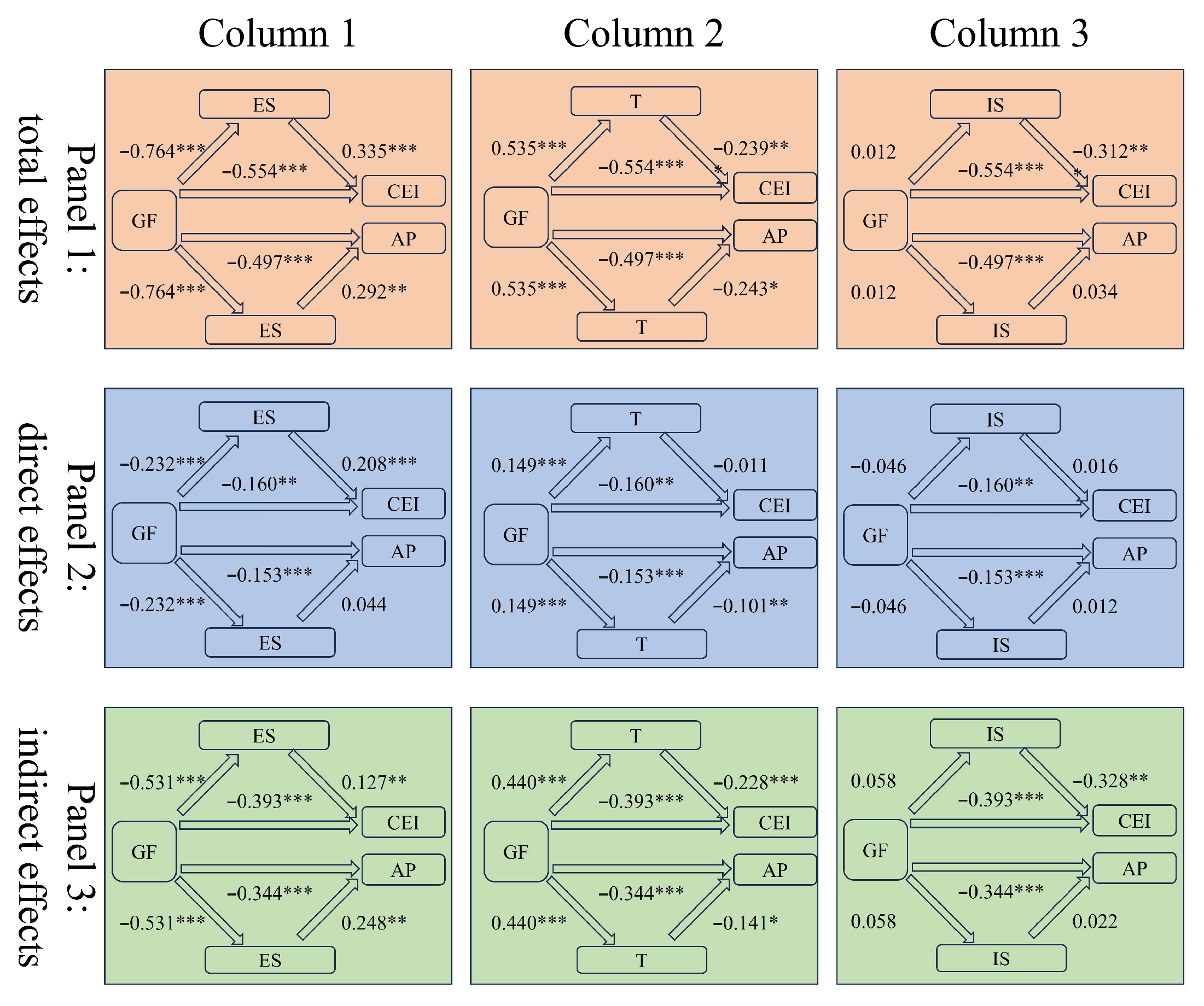
4.2. Mediation Path Analysis of GF on CE Intensity and AP

The estimation results of the spatial mediation effect model are shown in Figure 4. We calculated each mediation effect of ES, T, and IS in the pathways through which GF affects CEI and AP; the method is described in the Supporting Information, S6. The results of the mediation effects are shown in

Table 6. Results of the mediation effects.

Mediation Variables	Total Effect		Direct Effect		Indirect Effect
	GF on CEI	GF on AP	GF on CEI	GF on AP	GF on CEI	GF on AP
ES	0.462 *	0.449 *	0.302 *	0.067	0.172 *	0.383 *
T	0.231 *	0.262 *	0.001	0.098 *	0.255 *	0.18 *
IS	0.007	0.001	0.005	0.004	0.048	0.004

Note: * means that the mediation effect is significant at the 10% level. “GF on CEI” and “GF on AP” refer to the pathways through which GF affects CEI and through which GF affects AP, respectively.

.

From the view of total effect, GF reduces CEI and AP mainly by optimizing the ES and promoting the T. The coefficient of GF on IS is not significant (see Figure 4), indicating that GF does not significantly influence IS. According to Guan et al., environmental regulations effectively drive the transformation and upgrading of IS when levels of economic development and human capital are higher than a threshold [47]. Therefore, the insignificant impact of GF on IS may be due to the fact that China’s level of economic development and human capital has not reached the level at which GF significantly promotes the transformation and upgrading of IS. After decomposing the total effect, the direct effect of GF in reducing CEI is mainly through ES, and the spatial spillover effect of GF in reducing CEI is mainly through the spillover effect of T. However, the direct effect of GF in reducing CEI is mainly through T, and the spatial spillover effect of GF in reducing CEI is mainly through the spillover effect of ES.

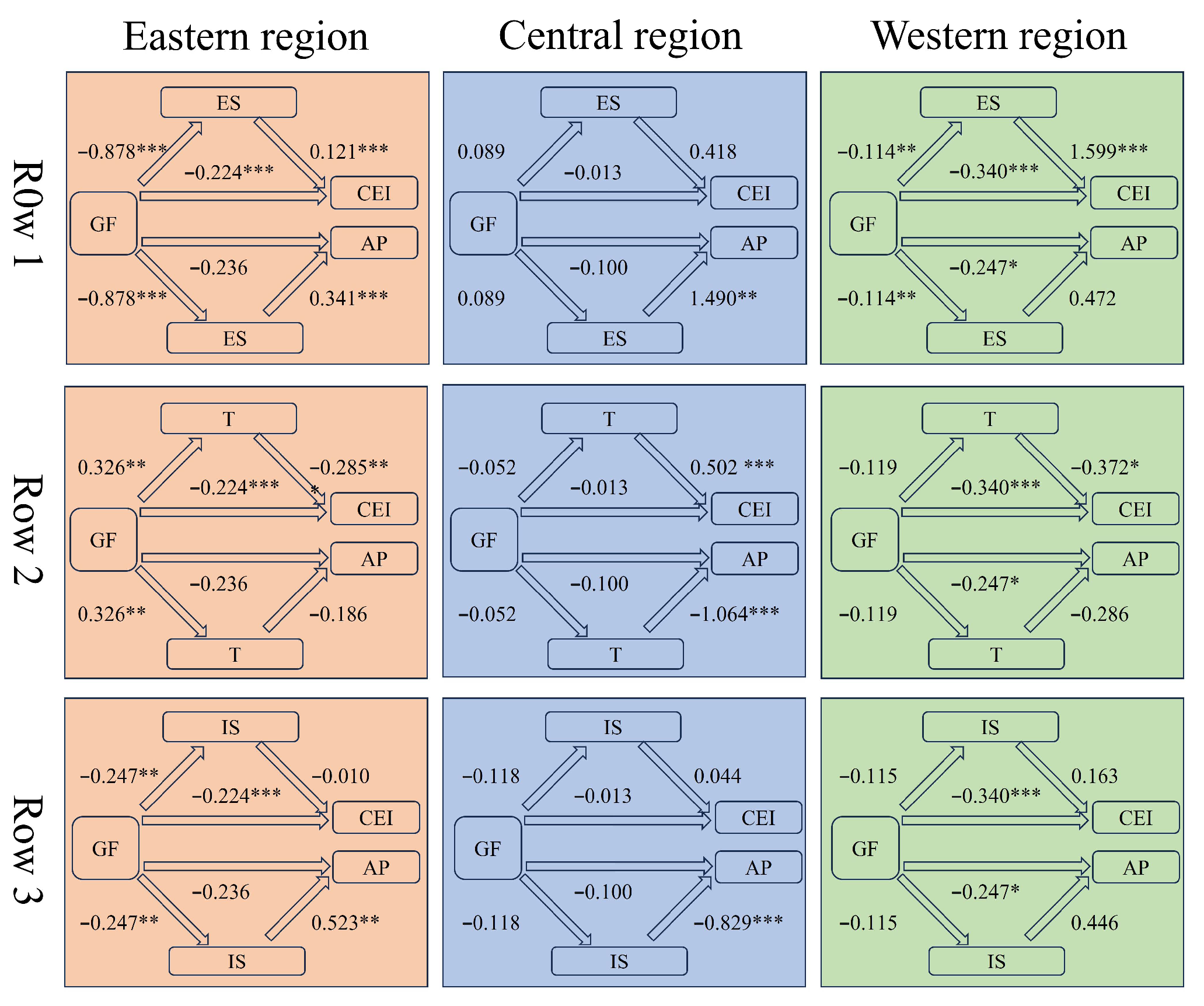
4.3. Analysis of Regional Heterogeneity of GF

In this study, we divided the 30 provinces (municipalities and autonomous regions) into Eastern, Central, and Western regions (Eastern region: Beijing, Fujian, Guangdong, Hebei, Jiangsu, Liaoning, Shandong, Shanghai, Tianjing, Zhejiang. Central region: Anhui, Hainan, Henan, Heilongjiang, Hubei, Hunan, Jilin, Jiangxi, Shanxi. Western region: GanSu, Guangxi, Guizhou, Inner-Mongolia, Ningxia, Qinghai, Shaanxi, Sichuan, Xinjiang, Yunnan, Chongqing) to conduct the heterogeneity analysis [48]. The results of the two-way fixed-effect SDM are shown in Figure 5 and Figure 6. In Figure 5, the total effect of GF on CEI and AP is significantly negative in the Western region but not in the Central region, and only the total effect of GF on CEI is significantly negative in the Eastern region.

Specifically in the Eastern region, both the direct effects of GF on CEI and AP are insignificant, the indirect effect of GF on CEI is significant, and the indirect effect of GF on AP is almost significant. This indicates that the non-significant direct effects of GF on CEI and AP are the main reasons for the non-significant total effect, which suggests that GF affects CEI and AP mainly through spillover effects. This result is the same as that of Zhou and Tang [46], who found that, with the development of GF in China, the environmental effects of GF transfer gradually from local to adjacent areas. In the Central region, direct and indirect effects were not significant, which means that the effect of GF is weak. In the Western region, both the direct effects of GF on CEI and AP are significantly negative, and only the indirect effect of GF on AP is non-significant. This proves that the impact of GF on CEI and AP in the Western region is mainly through direct effects, which suggests that the Western region is more sensitive to policies related to GF.

Furthermore, we explored the discrepancy in the pathways through which GF reduces CEI and AP in different regions based on the mediation effects model. The results are shown in Figure 6. Specifically in the Eastern region, the coefficients of GF on ES, T, and IS are −0.878, 0.326, and −0.247, respectively, at a 5% significant level. In the Central region, the coefficients are not significant. In the Western region, only the coefficient of GF on ES is significant. This reflects that the pathways of impact of GF on CE and AP vary dramatically across different regions.

5. Conclusions and Policy Recommendations

According to the previous literature, especially given the regional heterogeneity of China, the impacts of GF on CEI and AP and mechanisms of effects are certain and deserve further investigation. Therefore, we adopted the two-way fixed-effects spatial Durbin model and the spatial mediation effect model to explore the impact of GF on CEI and AP by exploiting panel data from 30 provinces in China between 2007 and 2019. Then, we further used a multiple spatial mediation effect model to discuss the specific path by which GF impacts CEI and AP, including the ES, T, and IS paths. Moreover, we analyzed the pathways of the impacts of GF on CEI and AP in the Eastern, Central, and Western regions of China. The conclusions of this study are as follows.

First, the results of the benchmark OLS regression, fixed-effects SDM, and robustness test prove that GF reduces CE while reducing AP. These results are consistent with most studies. This indicates that the continuous improvement and development of GF can reduce AP and CEI.

Second, the results of the indirect effects show that the spillover effect of GF cannot significantly reduce AP but can significantly reduce CEI. This is somewhat different from the results of the existing literature. According to a study by Zhou et al. [46], strict financing constraints on high-polluting enterprises lead to their transfer to regions with low GF development levels, resulting in GF in the surrounding regions playing an insignificant role in reducing local AP. This suggests that policymakers should focus on how green finance policies can comprehensively promote industrial reform and technological innovation, while strengthening environmental regulation and enforcement to avoid causing pollution transfer.

Third, the results of the mechanism analysis show that GF reduces AP and CEI mainly by promoting technological progress and ES optimization. This reveals that the government should guide and promote the development of GF to provide more financial capital for green technology and to increase the financing support for solar photovoltaic, wind, geothermal energy, and other clean renewable energy industries. However, the influence of GF on CEI and AP through IS is not significant, which is different from some results in the literature [28]. When studying the mechanism of GF’s effects on CEI and AP by region (see Figure 6), it was found that the impact of GF on IS in the Eastern region is significant, which implies that the effect of GF may be affected by the level of economic development [47]. The reason that it is not significant at the national level is likely to be that the adjustment of China’s industrial structure is more in favor of inter-regional transfer. This suggests that the government should encourage more capital to enter the green field, promote green transformation and upgrading of industrial structures, and try to maintain regional policy consistency to minimize green development due to the transfer of enterprises.

Finally, from a regional perspective, GF mainly reduces pollution and carbon through direct effects in the Western region of China and indirect effects in the Eastern region. This suggests that Western China is more sensitive to GF policies, which is different to what is suggested in other studies. The level of economic development in the Western region is relatively low, and many areas are dominated by more seriously polluting industries such as the chemical, mining, electric power, iron and steel industries, etc., which have relatively greater room for emission reduction; thus, by promoting the development of green finance, the provision of funds to promote the green transformation and upgrading of enterprises can effectively achieve pollution and carbon reduction. Policymakers should focus on supporting the development of GF in the Western region to directly reduce CEI and AP. From the perspective of the mechanism of GFs effects, the scope for reducing CEI and AP is relatively limited and can mainly be achieved by improving ES. Only in the Eastern region has it been found that GF also supports technological progress well. In the future, GF-supported areas should be more diversified, especially in the Central and Western regions.

This study also has some shortcomings. First, due to data limitations, the time period studied is 2007–2019, and more recent years are not analyzed. The data are also province-level, which cannot reflect the regional differences in a more detailed and adequate way. In recent years, especially after China’s double carbon goals were put forward, GF has increased dramatically in both scale and type, and its impact on environmental quality may also be increasing. In the next step, the research team will further obtain newer and more detailed data to study the effect of GF. Second, from a broader perspective, we have studied the effects of GF on pollution reduction and carbon mitigation separately, but academics and policymakers are more concerned about the co-benefits of affecting both. Although our research is helpful in understanding the co-benefits of pollution reduction and carbon mitigation, it is not specific enough to guide policymakers. Therefore, one of the directions of future research should be to explore the effect of GF on the co-benefits of pollution reduction and carbon mitigation.

References

1. Campbell-Lendrum, D.; Neville, T.; Schweizer, C.; Neira, M. Climate change and health: Three grand challenges. Nat. Med. 2023, 29, 1631–1638. [Google Scholar] [CrossRef] [PubMed]
2. Manisalidis, I.; Stavropoulou, E.; Stavropoulos, A.; Bezirtzoglou, E. Environmental and Health Impacts of Air Pollution: A Review. Front. Public Health 2020, 8, 13. [Google Scholar] [CrossRef] [PubMed]
3. Liu, Z.; Deng, Z.; He, G.; Wang, H.L.; Zhang, X.; Lin, J.; Qi, Y.; Liang, X. Challenges and opportunities for carbon neutrality in China. Nat. Rev. Earth Environ. 2022, 3, 141–155. [Google Scholar] [CrossRef]
4. Jiang, X.J. A conversation on air pollution in China. Nat. Geosci. 2023, 16, 939–940. [Google Scholar] [CrossRef]
5. Wang, X.Y.; Wang, Q. Research on the impact of green finance on the upgrading of China’s regional industrial structure from the perspective of sustainable development. Resour. Policy 2021, 74, 102436. [Google Scholar] [CrossRef]
6. Nedopil, C. Integrating biodiversity into financial decision-making: Challenges and four principles. Bus. Strateg. Environ. 2023, 32, 1619–1633. [Google Scholar] [CrossRef]
7. Zhang, T. Can green finance policies affect corporate financing? Evidence from China’s green finance innovation and reform pilot zones. J. Clean. Prod. 2023, 419, 138289. [Google Scholar] [CrossRef]
8. Shi, J.Y.; Yu, C.H.; Li, Y.X.; Wang, T.H. Does green financial policy affect debt-financing cost of heavy-polluting enterprises? An empirical evidence based on Chinese pilot zones for green finance reform and innovations. Technol. Forecast. Soc. Chang. 2022, 179, 121678. [Google Scholar] [CrossRef]
9. Lee, C.C.; Wang, F.H.; Chang, Y.F. Does green finance promote renewable energy? Evidence from China. Resour. Policy 2023, 82, 103439. [Google Scholar] [CrossRef]
10. Yuan, C.Q.; Liu, S.F.; Wu, J.L. Research on energy-saving effect of technological progress based on Cobb-Douglas production function. Energy Policy 2009, 37, 2842–2846. [Google Scholar] [CrossRef]
11. Zhao, X.S.; Fan, Z.H.; Ma, Y.J.; Gao, Z.Q. Research Review on Electrical Energy Storage Technology. In Proceedings of the 36th Chinese Control Conference (CCC), Dalian, China, 26–28 July 2017; pp. 10674–10678. [Google Scholar]
12. Azhgaliyeva, D.; Kapsalyamova, Z. Policy support in promoting green bonds in Asia: Empirical evidence. Clim. Policy 2023, 23, 430–445. [Google Scholar] [CrossRef]
13. He, X.B.; Shi, J.J. The effect of air pollution on Chinese green bond market: The mediation role of public concern. J. Environ. Manag. 2023, 325, 116522. [Google Scholar] [CrossRef] [PubMed]
14. Deng, Y.; Cui, Y.; Khan, S.U.; Zhao, M.J.; Lu, Q. The spatiotemporal dynamic and spatial spillover effect of agricultural green technological progress in China. Environ. Sci. Pollut. Res. 2022, 29, 27909–27923. [Google Scholar] [CrossRef] [PubMed]
15. Peng, B.H.; Sheng, X.; Wei, G. Does environmental protection promote economic development? From the perspective of coupling coordination between environmental protection and economic development. Environ. Sci. Pollut. Res. 2020, 27, 39135–39148. [Google Scholar] [CrossRef] [PubMed]
16. Chai, S.L.; Zhang, K.; Wei, W.; Ma, W.Y.; Abedin, M.Z. The impact of green credit policy on enterprises’ financing behavior: Evidence from Chinese heavily-polluting listed companies. J. Clean. Prod. 2022, 363, 132458. [Google Scholar] [CrossRef]
17. Pasupuleti, A.; Ayyagari, L.R. A Thematic Study of Green Finance with Special Reference to Polluting Companies: A Review and Future Direction. Environ. Process. 2023, 10, 24. [Google Scholar] [CrossRef]
18. Ameli, N.; Dessens, O.; Winning, M.; Cronin, J.; Chenet, H.; Drummond, P.; Calzadilla, A.; Anandarajah, G.; Grubb, M. Higher cost of finance exacerbates a climate investment trap in developing economies. Nat. Commun. 2021, 12, 4046. [Google Scholar] [CrossRef]
19. Desalegn, G.; Tangl, A. Enhancing Green Finance for Inclusive Green Growth: A Systematic Approach. Sustainability 2022, 14, 7416. [Google Scholar] [CrossRef]
20. Huang, J.B.; An, L.F.; Peng, W.H.; Guo, L.L. Identifying the role of green financial development played in carbon intensity: Evidence from China. J. Clean. Prod. 2023, 408, 136943. [Google Scholar] [CrossRef]
21. Zhang, W.; Zhu, Z.R.; Liu, X.M.; Cheng, J. Can green finance improve carbon emission efficiency? Environ. Sci. Pollut. Res. 2022, 29, 68976–68989. [Google Scholar] [CrossRef]
22. Purkayastha, D.; Sarkar, R. Getting Financial Markets to Work for Climate Finance. J. Struct. Financ. 2021, 27, 27–41. [Google Scholar] [CrossRef]
23. Hou, H.; Wang, Y.Y.; Zhang, M.L. Impact of environmental information disclosure on green finance development: Empirical evidence from China. Environ. Dev. Sustain. 2023, 31. [Google Scholar] [CrossRef]
24. Lan, J.; Wei, Y.M.; Guo, J.; Li, Q.M.; Liu, Z. The effect of green finance on industrial pollution emissions: Evidence from China. Resour. Policy 2023, 80, 103156. [Google Scholar] [CrossRef]
25. Zhang, A.L.; Wang, S.Y.; Liu, B. How to control air pollution with economic means? Exploration of China’s green finance policy. J. Clean. Prod. 2022, 353, 131664. [Google Scholar] [CrossRef]
26. Gao, J.; Wu, D.L.; Xiao, Q.; Randhawa, A.; Liu, Q.; Zhang, T. Green finance, environmental pollution and high-quality economic development-a study based on China’s provincial panel data. Environ. Sci. Pollut. Res. 2023, 30, 31917–31939. [Google Scholar] [CrossRef] [PubMed]
27. Jahanger, A.; Balsalobre-Lorente, D.; Ali, M.; Samour, A.; Abbas, S.; Tursoy, T.; Joof, F. Going away or going green in ASEAN countries: Testing the impact of green financing and energy on environmental sustainability. Energy Environ. 2023, 26, 0958305X231171346. [Google Scholar] [CrossRef]
28. Xu, X.Y.; Xie, Y.F.; Obobisa, E.S.; Sun, H.P. Has the establishment of green finance reform and innovation pilot zones improved air quality? Evidence from China. Hum. Soc. Sci. Commun. 2023, 10, 262. [Google Scholar] [CrossRef]
29. Xiang, W.M.; Qi, Q.; Gan, L. Non-linear effects of green finance on air quality in China: New evidence from a panel threshold model. Front. Ecol. Evol. 2023, 11, 1162137. [Google Scholar] [CrossRef]
30. Bai, J.C.; Chen, Z.L.; Yan, X.; Zhang, Y.Y. Research on the impact of green finance on carbon emissions: Evidence from China. Ekon. Istraz. 2022, 35, 6965–6984. [Google Scholar] [CrossRef]
31. Zeng, Q.; Tong, Y.J.; Yang, Y.Y. Can green finance promote green technology innovation in enterprises: Empirical evidence from China. Environ. Sci. Pollut. Res. 2023, 30, 87628–87644. [Google Scholar] [CrossRef]
32. Yao, S.J.; Zhang, X.Q.; Zheng, W.W. On green credits and carbon productivity in China. Environ. Sci. Pollut. Res. 2022, 29, 44308–44323. [Google Scholar] [CrossRef] [PubMed]
33. Li, W.A.; Cui, G.Y.; Zheng, M.N. Does green credit policy affect corporate debt financing? Evidence from China. Environ. Sci. Pollut. Res. 2022, 29, 5162–5171. [Google Scholar] [CrossRef] [PubMed]
34. Liu, X.H.; Wang, E.X.; Cai, D.T. Green credit policy, property rights and debt financing: Quasi-natural experimental evidence from China. Financ. Res. Lett. 2019, 29, 129–135. [Google Scholar] [CrossRef]
35. Wang, W.H.; Wang, X. Does provincial green governance promote enterprise green investment? Based on the perspective of government vertical management. J. Clean. Prod. 2023, 396, 136519. [Google Scholar] [CrossRef]
36. Nabeeh, N.A.; Abdel-Basset, M.; Soliman, G. A model for evaluating green credit rating and its impact on sustainability performance. J. Clean. Prod. 2021, 280, 124299. [Google Scholar] [CrossRef]
37. Diakoulaki, D.; Mavrotas, G.; Papayannakis, L. Determining objective weights in multiple criteria problems: The critic method. Comput. Oper. Res. 1995, 22, 763–770. [Google Scholar] [CrossRef]
38. Nie, X.; Chen, Z.P.; Wang, H.; Wu, J.X.; Wu, X.Y.; Lu, B.; Qiu, L.; Li, Y.Y. Is the “pollution haven hypothesis” valid for China’s carbon trading system? A re-examination based on inter-provincial carbon emission transfer. Environ. Sci. Pollut. Res. 2022, 29, 40110–40122. [Google Scholar] [CrossRef] [PubMed]
39. Shang, L.N.; Tan, D.Q.; Feng, S.L.; Zhou, W.T. Environmental regulation, import trade, and green technology innovation. Environ. Sci. Pollut. Res. 2022, 29, 12864–12874. [Google Scholar] [CrossRef]
40. Boamah, V.; Tang, D.C.; Zhang, Q.; Zhang, J.Q. Do FDI Inflows into African Countries Impact Their CO2 Emission Levels? Sustainability 2023, 15, 3131. [Google Scholar] [CrossRef]
41. Lu, L.; Liu, Z.; Mohsin, M.; Zhang, C.L. Renewable energy, industrial upgradation, and import-export quality: Green finance and CO2 emission reduction nexus. Environ. Sci. Pollut. Res. 2022, 30, 13327–13341. [Google Scholar] [CrossRef]
42. Anser, M.K.; Abbas, S.; Nassani, A.A.; Haffar, M.; Zaman, K.; Abro, M.M.Q. Innovative Carbon Mitigation Techniques to Achieve Environmental Sustainability Agenda: Evidence from a Panel of 21 Selected R&D Economies. Atmosphere 2021, 12, 1514. [Google Scholar] [CrossRef]
43. Ota, T. Economic growth, income inequality and environment: Assessing the applicability of the Kuznets hypotheses to Asia. Palgr. Commun. 2017, 3, 17069. [Google Scholar] [CrossRef]
44. James LeSage, R.K.P. Introduction to Spatial Econometrics; Chapman&Hall CRC Press: Boca Raton, FL, USA, 2009. [Google Scholar]
45. Lv, Z.K.; Li, S.S. How financial development affects CO2 emissions: A spatial econometric analysis. J. Environ. Manag. 2021, 277, 111397. [Google Scholar] [CrossRef] [PubMed]
46. Zhou, X.G.; Tang, X.M. Spatiotemporal consistency effect of green finance on pollution emissions and its geographic attenuation process. J. Environ. Manag. 2022, 318, 115537. [Google Scholar] [CrossRef]
47. Guan, S.; Liu, J.Q.; Liu, Y.F.; Du, M.Z. The Nonlinear Influence of Environmental Regulation on the Transformation and Upgrading of Industrial Structure. Int. J. Environ. Res. Public Health 2022, 19, 8378. [Google Scholar] [CrossRef]
48. Jiao, J.L.; Jiang, G.L.; Yang, R.R. Impact of R&D technology spillovers on carbon emissions between China’s regions. Struct. Chang. Econ. Dyn. 2018, 47, 35–45. [Google Scholar] [CrossRef]
Figure 1. Process framework. Different colors represent different aspects of our study.
Sustainability 16 01377 g001
Figure 2. Spatial distribution of provincial CEI, AP, and GF between 2007 and 2019. (a,b) show the spatial distribution of CEI, indicating that while CEI has been reduced overall, the reduction has been more pronounced in the Central and Eastern parts of the country; (c,d) demonstrate the spatial distribution of AP, showing that AP is higher in the Central region and lower in the Eastern region, with an overall decreasing trend; and (e,f) represent the spatial distribution of GF, suggesting that GF development levels increased in the East and decreased in the West.
Sustainability 16 01377 g002
Figure 3. Structural diagram of the multiple mediation effect model.
Sustainability 16 01377 g003
Figure 4. Mediation effects of GF on CEI and AP. *** p < 0.01, ** p < 0.05, and * p < 0.1. Panel 1-Panel 3 show the total, direct, and indirect effects of GF on CEI and AP, respectively. Column 1-Column 3 represent the three mediation pathways through which GF affects CEI and AP: ES, T, and IS.
Sustainability 16 01377 g004
Figure 5. The total effect of GF on CE and AP in different regions. (a,b) show the effects of GF on CEI and AP, respectively. If the error bars intersect with the horizontal zero reference line, it means that the effect is not significant; otherwise, it indicates that it is significant.
Sustainability 16 01377 g005
Figure 6. Pathways of the total effect of GF on CEI and AP in different regions. Row 1, Row 2, and Row 3 show the total effects of GF in reducing CEI and AP through ES, T, and IS, respectively. Note: *** p < 0.01, ** p < 0.05, and * p < 0.1.
Sustainability 16 01377 g006