Enhancing Streamflow Prediction Physically Consistently Using Process-Based Modeling and Domain Knowledge: A Review

Abstract

Streamflow prediction (SFP) constitutes a fundamental basis for reliable drought and flood forecasting, optimal reservoir management, and equitable water allocation. Despite significant advancements in the field, accurately predicting extreme events continues to be a persistent challenge due to complex surface and subsurface watershed processes. Therefore, in addition to the fundamental framework, numerous techniques have been used to enhance prediction accuracy and physical consistency. This work provides a well-organized review of more than two decades of efforts to enhance SFP in a physically consistent way using process modeling and flow domain knowledge. This review covers hydrograph analysis, baseflow separation, and process-based modeling (PBM) approaches. This paper provides an in-depth analysis of each technique and a discussion of their applications. Additionally, the existing techniques are categorized, revealing research gaps and promising avenues for future research. Overall, this review paper offers valuable insights into the current state of enhanced SFP within a physically consistent, domain knowledge-informed data-driven modeling framework.

1. Introduction

Streamflow—a vital element of the hydrological system—constitutes a pivotal nexus between the sustenance of diverse aquatic ecosystems and the fulfillment of fundamental human needs across agriculture, industry, and societal well-being [1,2,3]. It also plays a significant role in riverine processes, influencing erosion, transportation, and deposition. Additionally, streamflow serves as a critical indicator of climatic and environmental changes [4,5]. Therefore, accurate understanding and prediction of streamflow are essential for drought monitoring, infrastructure design, reservoir management, flood forecasting, water quality control, and water resource management [6,7]. However, despite advances in streamflow prediction (SFP) methods, accurate prediction remains challenging due to the complex interplay between natural and human influences on a watershed’s response to precipitation [6,8,9,10]. Land-use changes, water withdrawals, infrastructure development, topography, soil characteristics, and vegetation cover create a dynamic and interdependent system that challenges accurate modeling. Data limitations and measurement uncertainties further complicate the task [11,12].

Process-based models have been used to comprehend complex hydrological processes at the watershed scale, while data-driven modeling (DDM) has been used to predict streamflow by leveraging input–output relationships. DDM ranges from traditional statistical methods to complex artificial intelligence (AI)-based models, while process-based models encompass conceptual and physically based models [8,9,13]. Although less physically based, DDM often outperforms PBM in terms of predictive accuracy [14,15,16]. Developing physically based models is slow and requires extensive data, making DDM an attractive solution to the challenge of relating input and output variables in complex systems [17]. Moreover, DDM has the potential to avoid several sources of uncertainty in the modeling process, such as downscaling errors, hydrological model errors, and parameter uncertainty [12].

However, many operational forecasting agencies do not use DDM for SFP [18]. This may be due, in part, to the “black box” nature of DDMs, making it difficult to interpret predictions and diagnose errors [19]. Overfitting is also a significant concern in this paradigm, as the complexity of the models can lead to spurious relationships with the data [20,21]. In fact, both DDM and PBM paradigms have difficulty capturing extreme events, such as floods or prolonged droughts. While the inherent complexity and non-stationary nature of these events pose a significant challenge for any prediction model, the simplified hydrological processes often used in PBM frameworks further limit their accuracy [22]. For example, simplified representations of groundwater modules in watershed models or neglecting certain physical processes can hinder the models’ ability to capture the intricate dynamics of extreme events [23,24].

To improve SFP, several options, including domain knowledge, advanced data preprocessing techniques, multi-model integration, and metaheuristic algorithms, have been explored. While most of these techniques aim primarily to enhance prediction accuracy, PBM and domain knowledge-based approaches aim to improve prediction accuracy, interpretability, and physical consistency in a DDM framework. Incorporating domain knowledge as additional information about the mechanisms responsible for generating streamflow can help to build physically consistent models and improve model performance [14,25,26]. Additionally, integrating process-based models with data-driven models is recognized as a way to create a streamflow model that is both physically consistent and interpretable.

This comprehensive review delves into over two decades of research, beginning in 2002, focused on enhancing prediction accuracy by incorporating physical consistency and interpretability into the DDM framework. This paper begins by introducing the rationale and contribution of the review work. Next, it provides an overview of the rainfall-runoff process and modeling approaches. Subsequently, it presents a detailed review of major techniques used to improve the streamflow model. Following a comprehensive analysis of the literature review, the paper discusses its key points, identifies existing research gaps, and proposes potential future directions for further investigation. It concludes with a summary and outlook.

2. Rational and Contribution

Data-driven approaches have gained significant traction in hydrological modeling, prompting numerous review papers [27,28]. These reviews delve into various aspects of DDM in hydrology, including Artificial Neural Network (ANN) applications [17], general DDM techniques [8], AI applications in streamflow modeling [10], ensemble machine learning-based hydrological modeling [29], probabilistic modeling and post-processing [30], and hybrid deep learning-based streamflow forecasting [31].

The existing reviews on data-driven hydrological modeling primarily focus on updating model applications and algorithm explanations, leaving a gap in the understanding of physically consistent SFP enhancement techniques. This review addresses this gap by providing a comprehensive overview of these techniques and outlining a clear path forward. Moreover, as DDM has demonstrated superior prediction and forecasting capabilities, the focus has shifted from improving accuracy to ensuring physical consistency and interpretability. This review delves into the techniques developed to address these challenges and presents a roadmap for future research.

Enhancing SFP using physically consistent and domain knowledge-based approaches involves various techniques, often referred to as “physics-informed”, “expert knowledge-guided”, “hybrid”, and “integrated” models. This paper provides an overview of these techniques, highlighting their strengths, weaknesses, and challenges to improve data-driven model accuracy and reliability. Prediction is a broad term for guessing unseen variables, while forecasting is a specific term for predicting future variables based on time series data [30]. Nevertheless, since the techniques discussed in this paper can be applied to both prediction and forecasting, we use the general term “prediction” throughout.

3. Overview of Basic Watershed Processes and Streamflow Prediction

In the modeling paradigm, particularly within the context of PBM, detailed analysis and discussion of the distinct water balance segments and hydrological processes, along with comprehensive mathematical justifications and expert insights drawn from both the water balance and intimate familiarity with a study region, are crucial for strengthening the modeling procedures. Conversely, DDM can assist in circumventing certain modeling chain steps that involve uncertainty. Given the growing prevalence of the combined data-driven and PBM approach [12,32], this section provides an overview of both methods.

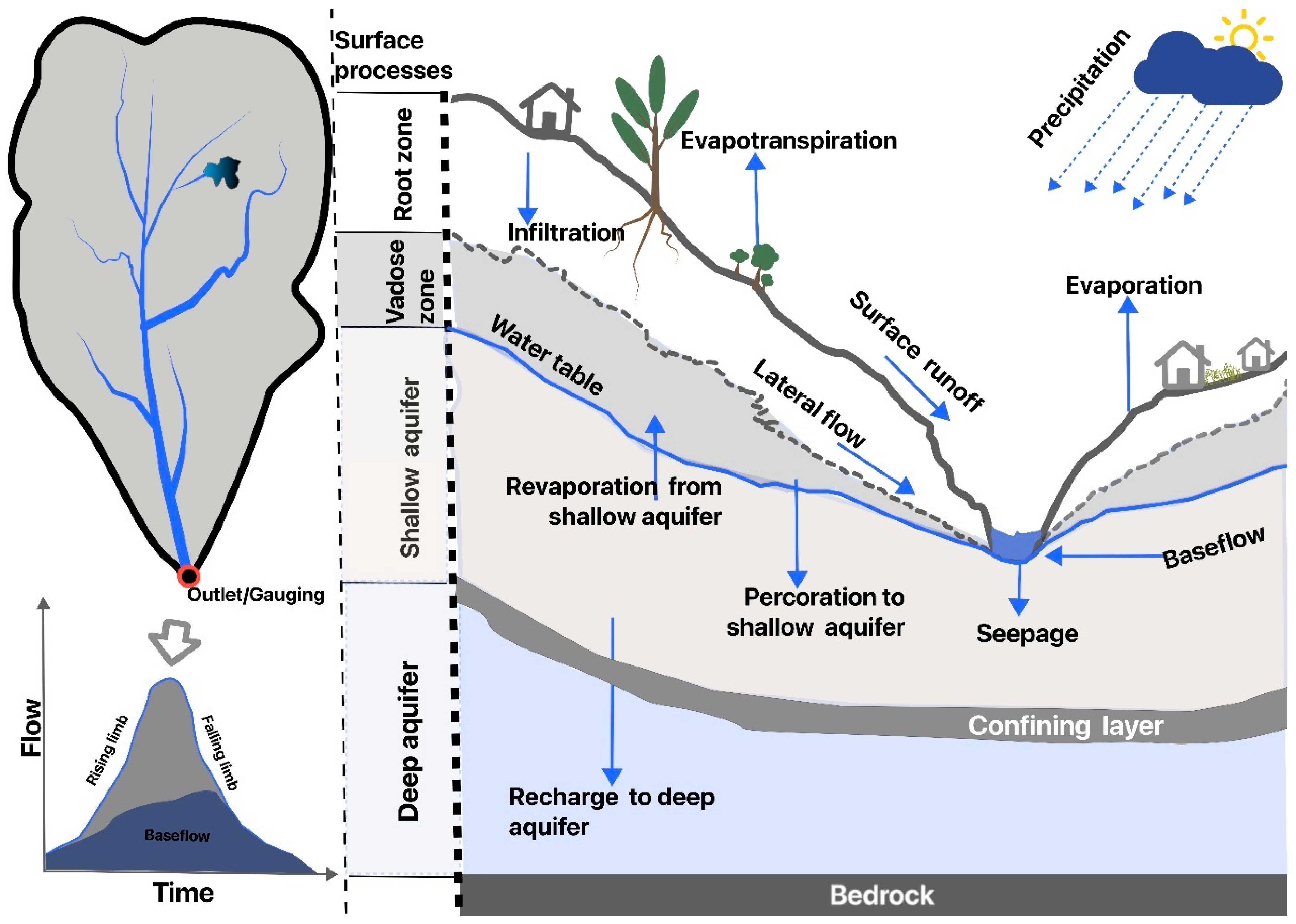
3.1. Streamflow Generation Processes

Several factors influence streamflow generation, such as climate, hydrogeology, soil properties, vegetation, management scenarios, and antecedent conditions. Precipitation undergoes interception by vegetation, infiltration into the soil, or surface runoff into streams. Evapotranspiration (ET) and subsurface processes, especially baseflow and lateral flow, significantly contribute to streamflow generation. From a watershed hydrology perspective, the generation is depicted based on their relation to surface processes, rootzone processes, and groundwater flow (Figure 1). However, conceptualizing and modeling streamflow has long been an intricate environmental challenge due to the significant subsurface flow mechanisms occurring in soil and bedrock, which we have limited capacity to quantify and evaluate [33].

3.2. Streamflow Prediction

PBM is typically used when there is a good understanding of the fundamental processes driving the system, and the goal is to create a model that accurately captures those processes. On the other hand, data-driven hydrological models use statistical or soft computing methods to map inputs to outputs without considering the physical hydrological processes involved in the transformation. The DDM approach is discussed further in Section 3.3. Examples of widely utilized PBM include the Soil and Water Assessment Tool (SWAT), HBV (Hydrologiska Byråns Vattenbalansavdelning) [34], GR4J (Génie Rural à 4 paramètres Journalier) [35], Variable Infiltration Capacity (VIC) [36], the Hydrologic Engineering Center–Hydrologic Modeling System (HEC-HMS) [37], and the Precipitation-Runoff Modeling System (PRMS) [38]. Next, we described the key hydrological processes and equations used in the SWAT model as an example of PBM.

The general SWAT model hydrological equation consists of four main water balance components—soil water, groundwater, ET, and surface runoff—which are simplified using the following relationships [39]:

$${SW}_t={SW}_0+\sum _{i=1}^t(R_i{-ET-Perc-Q_g-Q}_s)$$

(1)

where SW₀ and SW_t are the initial and final soil water content; t is time (days); and $R_i$, Q_s, Q_g, and Perc are the daily rainfall, surface runoff, groundwater discharge, and percolation. All units are in mm.

Each component of the general balance equation, commonly referred to as intermediate or state variables, is approximated using distinct relationships. The surface runoff in the above equation is computed using the commonly used SCS curve number procedure [40]:

$$Q_s=\frac{{\left(R_t-I_o\right)}^2}{\left(R_t-I_o+S\right)}$$

(2)

where R_t is the rainfall depth; I_o is the initial water abstraction in terms of surface storage, interception, and infiltration before runoff commences; and S is the retention parameter, which can be approximated using the following relationship, where CN is curve number:

$$S=25.4\left(\frac{1000}{CN}-10\right)$$

(3)

The groundwater component of the equation focuses on terms related to shallow and deep aquifers. The shallow aquifer contribution to the streamflow is approximated using the following relationship:

$$Q_{g,i}=Q_{g,i-1}.\mathrm{e}\mathrm{x}\mathrm{p}\left[{-\alpha }_{gw}·∆t\right]+w_{rchg}·\left(1-\mathrm{e}\mathrm{x}\mathrm{p}\left[{-\alpha }_{gw}·∆t\right]\right)$$

(4)

where $Q_{g,i}$ and $Q_{g,i-1}$ are the groundwater flow into the stream on day i and i − 1; ${\alpha }_{gw}$ is the baseflow recession constant; $∆t$ is the time step (1 day); and $w_{rchg}$ is water stored in the aquifer on day i.

The SWAT model ET computation relies on potential evapotranspiration (PET) and has multiple options. The selection of a method primarily depends on the availability of data. For instance, the Penman–Monteith method [41] necessitates measurements of solar radiation, air temperature, relative humidity, and wind speed, whereas the Hargreaves method [42] requires only air temperature data.

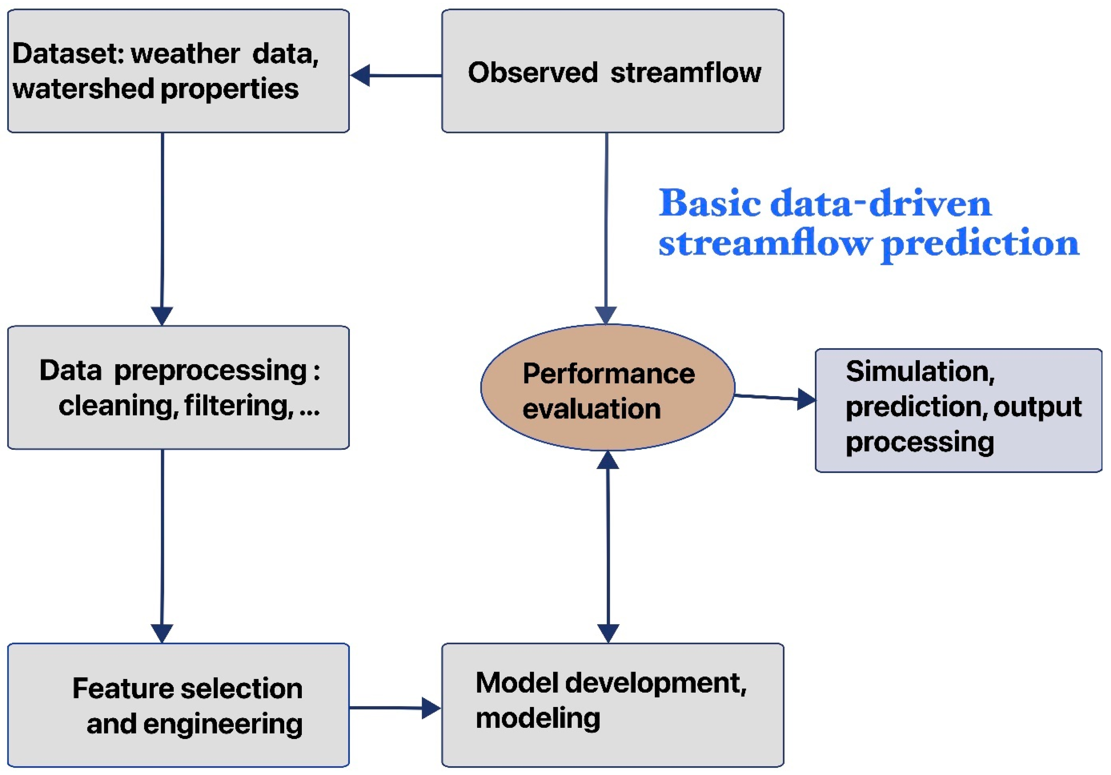
3.3. Basic Processes in Data-Driven Streamflow Prediction

DDM can be broadly classified into two types: conventional data-driven techniques and AI-based models [43,44]. Conventional techniques, such as multiple linear regression (MLR), autoregressive integrated moving average (ARIMA), autoregressive-moving average (ARMA), and autoregressive-moving average with the exogenous term (ARMAX), are preferred in SFP due to their simplicity. In contrast, AI-based models offer more advanced capabilities and higher accuracy [44,45]. The most widely utilized AI-based data-driven models fall into four categories: evolutionary algorithms, fuzzy-logic algorithms, classification methods, and artificial network techniques [10,45].

The basic steps in DDM include data preprocessing, selecting suitable inputs and architecture, parameter estimation, and model validation [46,47,48]. This procedure unfolds in four key steps: data collection and cleaning, feature selection and engineering, model selection and building, and prediction (Figure 2). Effective data preprocessing, which typically involves essential steps such as data cleaning to detect and correct anomalies or inconsistencies, is critical for DDM as it significantly impacts subsequent analysis accuracy and efficiency [47]. To ensure the model’s ability to generalize to real-world scenarios, a crucial step is to divide the available data into three distinct subsets: training, testing, and validation [49]. This strategic division allows the model to learn from the majority of the data during training, undergo a rigorous evaluation on a separate testing set, and finally, have its ability to generalize to unseen data confidently validated [50].

Utilizing multiple input variables in hydrologic and water resources applications poses a challenge in identifying the most relevant or significant ones [48,51]. Selecting the most pertinent features can enhance model accuracy, mitigate overfitting, and improve the interpretability of natural processes [47,51,52]. Feature selection encompasses a variety of techniques, including filtering, wrapper, and embedded methods, which are broadly classified into model-free and model-based approaches [52,53,54].

An ideal input selection algorithm should exhibit flexibility for modeling, computational efficiency for handling high-dimensional datasets, scalability with respect to input dimensionality, and redundancy minimization [52]. A primary drawback of the model-based method lies in its computational demands, as it necessitates numerous calibration and validation processes to identify the optimal input combination. This renders the method unsuitable for large datasets [54]. Moreover, the input selection outcome hinges on the predetermined model class and architecture. Nonetheless, model-based approaches generally achieve superior performance due to their fine-tuning to the specific interactions between the model class and the data.

Feature engineering, the process of preparing input data before training a neural network, offers several benefits: reduced error in estimated outcomes, shorter training times, and equal attention to all data [55]. Effective normalization involves converting data to a linear scale, where equal relative changes correspond to identical absolute values [56]. Data are typically adjusted to fit within ranges like [–1, 1], [0.1, 0.9], or [0, 1] [56,57].

A comprehensive evaluation of a hydrological prediction model’s performance requires both graphical and numerical analyses of its error relative to observed data, including the selection of appropriate performance criteria and careful interpretation of the results [58]. For a more holistic assessment, it is recommended to use at least one goodness-of-fit measure, such as the Nash–Sutcliffe Efficiency Coefficient (NSE) [59], and one absolute error measure, such as root mean square error (RMSE) [60]. Specifically, for DDM, the relative correlation coefficient is recommended as an alternative to conventional evaluation measures such as NSE [60].

4. Enhancing Streamflow Prediction Using a Physically Consistent and Domain-Aware Approach

Having established the efficacy of DDM, the scientific community is now focusing on refining model structures and techniques to improve the reliability, clarity, and physical coherence of DDM for decision-makers [8,26]. Numerous pioneering strategies have been proposed to advance the field of hydrology through a data-centric lens. Among these, the most pervasive and avant-garde approaches involve fusing PBM with DDM, commonly referred to as physics-informed DDM, and judiciously incorporating domain expertise, as exemplified by hydrograph analysis (Figure 3).

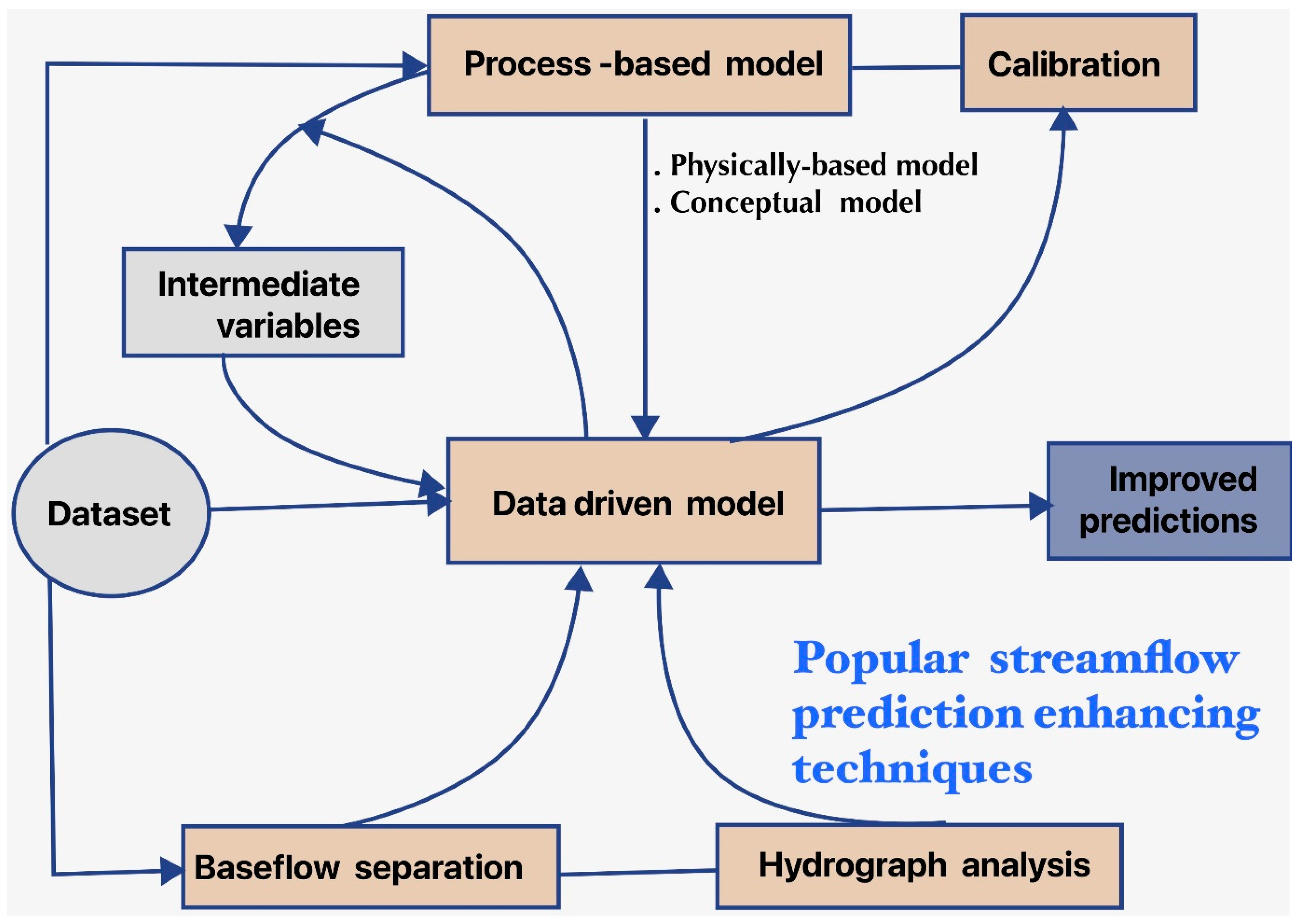
4.1. Process Modeling Approach for Improved Streamflow Prediction in the Data-Driven Modeling Framework

To develop physically consistent data-driven streamflow models, various hydrological models, ranging from large-scale models like the United States National Water Model (NWM) [61] and the Weather Research and Forecasting hydrological model (WRF-Hydro) [62], to simpler models like the Tank model [63], MISDc (Modello Idrologico Semi-Distribuito in continuo) [64], and Soil Moisture Accounting and Routing (SMAR) [65], have been coupled with different data-driven models. SWAT, HBV, and GR4J are widely used models (Table 1). Additionally, models commonly used in water resource management, such as Water Evaluation and Planning (WEAP) [66] and Non-Recorded Catchment Areas (NRECA) [67], are also integrated with data-driven models.

Although uncommon, PBM has been used to simulate streamflow data as a target variable, as demonstrated by Yang et al. [68], who used a geomorphology-based hydrological model (GBHM) [69] to simulate streamflow. Moreover, with various objectives, SIMHYD [70], Identification of unit Hydrographs And Component flows from Rainfall Evapotranspiration and Streamflow data (IHACRES) [71], HYMOD [72], Sacramento soil moisture accounting model (SAC-SMA) [73], and GR2M model [74] have been used in conjunction with data-driven models.

Commonly, five approaches have been used to add physical consistency to data-driven SFP: (1) introducing intermediate variables simulated by the process-based model into the data-driven model or replacing a selected PBM module with a data-driven model; (2) training the data-driven model using the hydrological model residual error; (3) using the process-based simulated streamflow directly as input for the data-driven model; (4) parameterization; and (5) combining the outputs of both models as input for the data-driven model. Calibrating key parameters of process-based models with the help of machine learning algorithms is also emerging as a powerful approach for enhancing model performance. The model can either be single learner-based or an ensemble approach. This framework leverages a diverse array of advanced machine learning models, from traditional approaches including Light Gradient Boosting Machines (LGB), eXtreme Gradient Boosting Machines (XGB), Generalized Linear Models (GLMs), Gaussian Process Regression (GPR), Extremely Randomized Trees (Extra-Trees), and K-Nearest Neighbor Regression (KNN), to powerful deep learning architectures like Convolutional Neural Networks (CNNs), LSTM, and ANNs.

4.1.1. Introducing Intermediate Variables

As highlighted in Section 3, complex hydrological and hydrogeological processes are typically represented using various modules in process-based models. These modules yield intermediate variables, each contributing differently to streamflow generation. Incorporating these simulated variables, along with climate forcing, into the DDM framework enhances SFP by capturing catchment memory and environmental water requirements (Figure 4). For instance, incorporating a conceptual infiltration equation considering changing soil moisture conditions and effective rainfall into the input vector can reduce runoff prediction errors due to initial watershed conditions [75].

Noori and Kalin [76] improved summer season SFP accuracy by incorporating baseflow and stormflow simulated by the SWAT model into an ANN. Similarly, Humphrey et al. [77] demonstrated that including the GR4J simulated soil moisture index enhanced the peak flow computation performance of a Bayesian ANN. Ren et al. [78] introduced the HBV model-simulated initial snowmelt and glacier-melt runoff into a Bayesian ANN to increase SFP accuracy in cold regions (Central Asia). The authors found improved model performance and reasonable uncertainty intervals. In another related approach, Bhasme et al. [79] computed ET using an ABCD model [80] and used it as input for several regression models, including support vector machines for regression (SVR), GPR, Lasso, and ridge. The hybrid model outperformed both the process-based and data-driven models. Xu et al. [81] used the Utah Energy Balance (UEB) snow model [82] with a conventional long short-term memory (LSTM) model in a snow-dominated region of the USA. The authors conducted a comparative analysis of the proposed approach against the LSTM, Random Forest (RF), and SAC-SMA models. The results indicated that the proposed model exhibited superior performance and reasonable spatiotemporal recharge–discharge patterns.

4.1.2. Combining Data-Driven and Process-Based Model Outputs

A few studies have utilized a combination of process-based and data-driven models to improve the performance of the latter [83,84]. This technique has been utilized as a potential solution to address data scarcity [84]. Farfán et al. [83] combined the outputs of WEAP and GR2M with ANN models, which used different inputs. The PBM output-incorporated data-driven model demonstrated superior performance in predicting peak flows and consistency between the calibration and validation phases compared with the individual models. Mohammadi et al. [84] evaluated various combinations of process-based (HBV and NRECA) and data-driven models—Adaptive Neuro-fuzzy Inference System (ANFIS) and support vector machine (SVM)—and used the group method of data handling (GMDH) toward improved prediction.

4.1.3. Residual Error Modeling

Residual error modeling encompasses both error identification and uncertainty estimation in Bayesian and statistical techniques, as well as the connection of hydrological model errors to DDM [85,86,87]. This approach, widely used in integrating process-based and data-driven models, involves recognizing and understanding biases within process-based models compared with real observations. This information is subsequently utilized to rectify model outcomes [88]. In Equation (5) [89], hydrological model error is simplified (${\epsilon }_t$), with t representing time, $Q_t$ denoting observed discharge, $f\left(x_t;\theta \right)$ representing model-simulated discharge, $x_t$ representing forcing data, and $\theta$ representing a set of unknown model parameters.

$$Q_t=f\left(x_t;\theta \right)+{\epsilon }_t$$

(5)

This method has been used for SFP enhancement in two ways (Figure 5). The first involves training a data-driven model solely on PBM error. The second approach involves incorporating the PBM error as one of several input variables [20,85,90]. Tian et al. [90] introduced GR4J residual error along with other input datasets into an LSTM model and a nonlinear autoregressive exogenous input neural network (NARX). Cho and Kim [20] used a related method: they trained an LSTM model using WRF-Hydro residual error and meteorological forcing data and then aggregated the PBM-predicted streamflow with the LSTM model residual error prediction. Han and Morrison [91] used numerical weather model (NWM) prediction errors and precipitation as inputs for LSTM, achieving enhanced prediction accuracy in both temporal accuracy and the volume of computed flow. Similarly, Yang et al. [92] enhanced SWAT+ prediction considering snowmelt using a residual modeling approach with a Gated Recurrent Unit (GRU) model, which outperformed individual models. Kassem et al. [93], on the other hand, followed the first approach: they used the SWAT model residual error as input for an ANN.

Choosing between calibrated and uncalibrated models for residual error use is essential. Shen et al. [94] evaluated the potential for both calibrated and uncalibrated versions of the PCRaster Global Water Balance (PCR-GLOBWB) model to improve performance when integrated with RF. The results showed significant improvements in predictive accuracy for both models when coupled with RF.

Roy et al. [95] recently proposed a dynamic error-correction approach for streamflow forecasting using an RF model with the HBV model. The framework demonstrated consistent accuracy, especially for long lead time and low flow predictions. In a subsequent study [96], the authors evaluated different scenarios, such as using only weather data, only intermediate variables prediction intervals, only SFP intervals, or all these variables together. They found that simulations incorporating all variables outperformed the others consistently.

4.1.4. Simulated Streamflow as Input

PBM-simulated streamflow has been used as an input variable in the DDM framework, primarily to address data scarcity and improve accuracy. This involves combining hydrological model output using data from various sources or merging different hydrological model simulation results using the same input data or both [21,32,62,97,98,99]. Additionally, hydrological model-simulated subbasin-scale results have been utilized to enhance predictions at the outlet of the watershed or as a routing technique [100,101,102].

Song et al. [101] extended a previous study [100], which combined the XinAnJiang (XAJ) model [103] with an ANN. They used the output of the XAJ model at each subbasin as input for the ANN. Liu et al. [104] used the coupled XAJ and TOPMODEL [105] models as weak learners to improve SFP using the Adaptive Boosting (AdaBoost) algorithm. This hybrid approach excelled in low-flow predictions. Mekonnen et al. [106] addressed the challenge of accounting for “contributing” and “non-contributing” areas in physical models by combining SWAT for contributing regions and raw data with an ANN for non-contributing areas, which enhanced discharge simulation. Within the same modeling framework, Liu et al. [107] used the coupled VIC and Catchment-based Macro-scale Floodplain (CaMa-Flood) [108] model output as input for the LSTM in addition to meteorological data to improve prediction performance. Zhou et al. [109] used XAJ model outputs as input for the Monotone Composite Quantile Regression Neural Network (MCQRNN) to enhance flood forecasting. The results indicated that XAJ-MCQRNN outperformed the MCQRNN model forecasts.

For post-processing, this approach was used to combine outputs from multiple simulations or models with different data sources. For example, Thalli Mani et al. [110] built a SWAT model with diverse metrological data and used data-driven models to assemble streamflow data. Li et al. [111] processed SWAT, VIC, and TOPMODEL with Muskingum–Cunge routing (BTOPMC) [112] outputs using an ANN to obtain an enhanced prediction.

Recent studies have compared the performance of various models using the approach of integrating PBM-simulated streamflow into DDM. For instance, Parisouj et al. [113] evaluated the performance of three machine learning models—extreme learning machine (ELM), SVR, and LSTM—alongside the HEC-HMS model and a hybrid model that combined the LSTM model with HEC-HMS. Their results showed that the hybrid model produced the best outcomes. Vidyarthi and Jain [102] used nonlinear regression (NLR) and ANN in the Australian Water Balance Model (AWBM) [114] to simulate rainfall–runoff processes. Their findings showed that integrating an ANN with the AWBM, particularly when incorporating time-lagged runoff as an input variable, resulted in the highest performance. Zhong et al. [115] used VIC model output as input for CaMa–Flood and integrated climate data and model outputs into both recurrent neural networks (RNNs) and LSTM models. Their results indicated that the LSTM model using hydrological model outputs outperformed the other models. Studies also show that, in general, this approach performs better than residual modeling [116,117]. However, Frame et al. [61] found that including NWM output with atmospheric data in the LSTM model yielded similar results to the LSTM model trained only with atmospheric data.

A few studies have explored the impact of calibrated and uncalibrated model outputs and the incorporation of additional forcing data on prediction performance. S. Yang et al. [118] coupled calibrated and uncalibrated SWAT models with LSTM. The calibrated SWAT model coupling outperformed the uncalibrated and individual models. Exploring the impact of additional climate-forcing variables, Achite et al. [119] combined the MISD model with the GMDH, incorporating MISD-simulated streamflow and various meteorological variables as inputs. Their results demonstrate enhanced model performance due to the inclusion of additional meteorological forcing variables.

4.1.5. Replacing Process-Based Model Modules

PBMs often comprise some modules that lack detailed physical process representation, depending on their focus. One technique to improve flow prediction in a physically consistent way is to replace one or more of these modules with machine learning algorithms. This technique has been practiced in two ways. The traditional approach substitutes PBM modules with externally calculated intermediate variables (e.g., ET). A more advanced method uses algorithms that incorporate physical processes [120,121,122]. Even substituting the common routing module with a data-driven model can improve model performance compared with using PBM-simulated outputs at outlets and subbasins [121]. Recent developments in physics-wrapped neural networks have enhanced both interpretability and efficiency. The widely tested Process-Wrapped Recurrent Neural Network (P-RNN) approach is commonly applied alongside the EXP-HYDRO model [123] for parametrization or module replacement [122,124,125,126].

For example, Jiang et al. [124] integrated P-RNN with EXP-HYDRO to improve SFP, achieving robust transferability and an enhanced ability to infer unobserved processes. Feng et al. [127] developed differentiable hydrological models using embedded neural networks (ENNs) for parameterization or module replacements using Differentiable Parameter Learning (dPL). Their framework achieved prediction accuracy comparable to LSTM models. Höge et al. [125] introduced a hydrologic neural ordinary differential equation (ODE) to enhance prediction accuracy while preserving interpretability. Their framework demonstrated significant performance improvement when tested with EXP-HYDRO. Li et al. [122] further investigated P-RNN alongside EXP-HYDRO, exploring the replacement of EXP-HYDRO modules with ENNs. They found that using ENNs improved SFP, but replacing multiple modules did not consistently yield further improvements. Using a traditional approach, Lian et al. [120] replaced the ET module of the XAJ and SWAT models with RF. Their results showed that RF-XAJ outperformed the original XAJ model, while the SWAT and RF-SWAT models performed equally.

4.1.6. Model Calibration

Utilizing machine learning algorithms to update hydrological model parameters has demonstrated comparable effectiveness in enhancing model accuracy compared to established techniques based on residual error and simulated flow-related adjustments [87,128,129,130]. For instance, Yu et al. [131] investigated three integration approaches combining the HBV model and LSTM. The first approach used HBV-simulated streamflow and meteorological data as input for LSTM. The second approach integrated meteorological data and HBV-simulated streamflow for error correction within LSTM. The third approach utilized meteorological data and HBV-simulated streamflow to update HBV model parameters using LSTM. All three approaches outperformed the individual models, with the third approach exhibiting superior performance. Jiang et al. [129] proposed a knowledge-informed inverse mapping technique that estimates each parameter using only responses that share significant mutual information with the parameter. This approach demonstrates the potential for incorporating domain knowledge into machine learning algorithms for hydrological parameterization.

Table 1. Summary of the reviewed works that couple PBM with data-driven models to enhance prediction accuracy. Input variables for embedded neural networks or differentiable physics-informed machine learning approaches are not described here (*).

Process-Based Model	DD Model	Study Region	Input Variables	Authors	Findings/Remarks
GR4J, modified IHACRES and TOPMODEL	ANN	France	Rainfall, streamflow, error	[88]	The hybrid model outperformed all the other models for 3-day forecasts.
XAJ, SMAR, Tank model	ANN	China	Streamflow	[100]	The coupled modeling approach excelled over the individual models.
HBV	ANN	Meuse River basin	Precipitation, streamflow	[121]	The conceptual data-driven model approach enhanced low-flow prediction.
XAJ	ANN	China	Subbasin discharge	[101]	XAJ-ANN yielded more reasonable results.
XAJ, TOPMODEL	AdaBoost	China	Streamflow	[104]	Enhanced low flow prediction performance was obtained.
HEC-HMS	ANN	Taiwan	Precipitation, runoff	[132]	The hybrid model showed improved discharge prediction.
SWAT	ANN	Canada	Streamflow, climate	[106]	SWAT-ANN outperformed the individual models.
SWAT	ANN	USA	Baseflow, excess flow	[76]	Enhanced flow predictions in ungauged watersheds was achieved.
GR4J	ANN	Australia	Streamflow, precipitation, GR4J simulated soil moisture index, PET	[77]	High peak flow performance was observed.
HEC-HMS	SVM, ANN	Taiwan	Streamflow, precipitation	[97]	The HEC-HMS-SVR model provided the most accurate discharge.
GR4J	LSTM, NARX	China	Error, precipitation, PET	[90]	GR4J with LSTM and NARX excelled for smaller catchments.
HBV, GR4J, SIMHYD	MLR, Extra-Trees, LGB, XGB	Central Asia	Runoff, PET, climate	[133]	Acceptable results were achieved in ungauged regions.
HBV	ANN, SVM	China	Climate, simulated runoff	[78]	HBV-ANN was more reliable and accurate for high-flow predictions.
SWAT, VIC, BTOPMC	ANN	China	Streamflow	[111]	Enhanced low and peak flow prediction were achieved.
NWM	New assessment tool	USA	*	[134]	The tool accurately predicted hydrographs across rising and recession phases, demonstrating exceptional performance.
SAC-SMA	LSTM	USA	Residual error, streamflow, climate	[116]	The hybrid model enhanced the performance of SAC-SMA but struggled in catchments with prolonged low-flow conditions.
HYMOD	ANN	USA	Streamflow, PET, climate	[99]	The hybrid model enhanced flow prediction.
SWAT	ANN	Iraq	Residual error	[93]	SWAT-ANN surpassed the SWAT model.
WEAP, GR2M	ANN	Ecuador	Streamflow, precipitation, PET	[83]	Enhanced peak flow forecasting with reliable performance across calibration and validation stages.
SWAT, HEC-HMS	ANN	USA	Streamflow, precipitation	[98]	The hybrid model enhanced long-term forecasting and enabled SFP based on forecasted rainfall.
GBHM	ANN	Thailand	Synthetic runoff, spatial inputs	[68]	Improved peak flow prediction and boosted model performance in data-scarce regions.
EXP-HYDRO	P-RNN	USA	*	[124]	The method accurately inferred unobserved phenomena.
SWAT	ANN	Iran	Residual error	[117]	SWAT-ANN performed better than SWAT.
TOPMODEL	Boosting method	China	Precipitation, runoff	[135]	The ensemble approach performed better than TOPMODEL both in humid and semi-arid regions.
HBV, NRECA	ANFIS, SVM, GMDH	Indonesia	Precipitation, streamflow	[84]	The hybrid model outperformed the hydrological models, with GMDH excelling in peak flow prediction.
PRMS	LSTM	USA	Streamflow, climate	[21]	The hybrid model excelled, but its performance hinged on the process-based model’s performance.
NWM	LSTM	USA	NWM outputs, catchment attributes, climate	[61]	LSTM improved NWM predictions.
HBV	KNN, MLR, SOV, ANN, XGB, RF	Swiss	Residual error, streamflow, climate	[85]	HBV-XGB and HBV-RF performed best.
WRF-Hydro	LSTM	Korea	Residual error, climate	[20]	WRF-Hydro-LSTM outperformed the individual models.
SWAT	RF, ANN, GLM, gradient boosting, KNN, Cubist	India	Streamflow, climate	[110]	Ensemble streamflow-based prediction outperformed the other models.
ABCD	SVR, GPR, Lasso, Ridge regression	India	ET, groundwater storage, soil moisture, precipitation	[79]	The hybrid model excelled beyond the process-based and data-driven models and maintained a reasonable water balance.
HBV	RF, XGB	Swiss	Streamflow, climate	[136]	The hybrid model performed better.
IHACRES, GR4J, MISD	MLP, SVM	Swiss	Runoff, climate	[32]	The process-based models’ performance increased by 19%.
HBV	dPL	USA	*	[127]	Differentiable, physics-based models achieved performance comparable to LSTM models.
XAJ	MCQRNN	China	Rainfall, observed and simulated flow	[109]	XAJ-MCQRNN outperformed MCQRNN on interval and point flood forecasts.
EXP-HYDRO	Neural ODE	USA	*	[125]	Improved and interpretable results were obtained.
VIC, CaMa-Flood	LSTM	Lancang–Mekong River	Climate, simulated streamflow	[107]	LSTM using hydrologic model output improved prediction.
AWBM	NLR, ANN	USA	Runoff	[102]	Using ANN to route within the conceptual model improved predictions, especially with delayed runoff as input.
UEB	LSTM	USA	Simulated snowmelt and rainfall, PET	[81]	The coupled approach outperformed benchmark models and yielded reasonable spatiotemporal recharge–discharge distribution.
HEC-HMS	ELM, SVR, LSTM	Iran	Climate, observed and simulated discharge	[113]	HEC-HMS-LSTM outperformed all other models.
HYMOD, SAC-SMA, VIC	LSTM	USA	Climate, watershed characteristics, simulated ET	[137]	Performance depended on the process-based model.
NWM	LSTM	USA	Residual error, precipitation	[91]	LSTM significantly boosted NWM prediction accuracy, enhancing both temporal precision and streamflow volume.
MISD	GMDH	Sweden	Climate, MISD model result	[119]	Including more metrological forcing enhanced hybrid model performance.
PCR-GLOBWB	RF	Rhine basin	Climate, intermediate variables, error	[94]	RF error correction significantly enhanced SFP, with calibrated and uncalibrated error correction yielding equally accurate results.
TOPMODEL	ARIMA, LSTM, Prophet	China	Residual error	[138]	The integrated approach enhanced flow prediction, with the Prophet model performing the best.
HBV	RF	India, Nepal	Error, observed and simulated streamflow	[95]	HBV-RF prediction excelled over HBV, enhancing low-flow prediction.
HBV	RF	India, Nepal	Error, intermediate variables, weather data	[96]	The HBV-RF model excelled in performance, especially when weather and simulated streamflow data were incorporated.
SWAT	LSTM	China	Climate, intermediate variables	[139]	SWAT-LSTM excelled over SWAT and LSTM, demonstrating efficiency in poorly gauged watersheds.
PCR-GLOBWB	RF	Global	Intermediate variables, static predictors, PCR-GLOBWB model inputs	[140]	Including hydrological model outputs improved SFP.
HBV	LSTM	China	Climate, simulated streamflow	[131]	Combining HBV with LSTM enhanced prediction accuracy, where tight coupling was the more efficient approach.
GR4J	CNN, LSTM	Australia	Intermediate variables, observed streamflow, climate data	[141]	The integrated model outperformed the individual models, particularly excelling in arid catchments.
SWAT	LSTM	Malaysia	Precipitation, simulated streamflow	[118]	Coupling the calibrated SWAT model with LSTM improved SFP.
EXP-HYDRO	ENN	USA	*	[122]	The EXP-HYDRO with ENN outperformed the conceptual model, yielding physically consistent results.
SWAT+	GRU	China	Climate, Residual error	[92]	SWAT+ glacier error corrected using GRU improved low- and peak-flow predictions.
VIC, CaMa-Flood	RNN, LSTM	China	Climate, simulated flow	[115]	LSTM combined with the hydrologic model achieved superior performance.
XAJ, SWAT	RF	USA	*	[120]	RF with XAJ enhanced prediction performance, while SWAT and RF-SWAT exhibited comparable accuracies.
EXP-HYDRO	P-RNN	China	*	[126]	The physics-informed deep learning model surpassed EXP-HYDRO in permafrost-affected alpine catchments under climate change conditions.
HBV	dPL	USA	*	[142]	For ungauged regions, differentiable physics-informed machine learning outperformed LSTM. Suitable for climate change assessment.
NWM	ANN	USA	Streamflow, soil, land use, topography	[62]	The hybrid model improved the forecast reliability significantly.

Table 1. Summary of the reviewed works that couple PBM with data-driven models to enhance prediction accuracy. Input variables for embedded neural networks or differentiable physics-informed machine learning approaches are not described here (*).

Process-Based Model	DD Model	Study Region	Input Variables	Authors	Findings/Remarks
GR4J, modified IHACRES and TOPMODEL	ANN	France	Rainfall, streamflow, error	[88]	The hybrid model outperformed all the other models for 3-day forecasts.
XAJ, SMAR, Tank model	ANN	China	Streamflow	[100]	The coupled modeling approach excelled over the individual models.
HBV	ANN	Meuse River basin	Precipitation, streamflow	[121]	The conceptual data-driven model approach enhanced low-flow prediction.
XAJ	ANN	China	Subbasin discharge	[101]	XAJ-ANN yielded more reasonable results.
XAJ, TOPMODEL	AdaBoost	China	Streamflow	[104]	Enhanced low flow prediction performance was obtained.
HEC-HMS	ANN	Taiwan	Precipitation, runoff	[132]	The hybrid model showed improved discharge prediction.
SWAT	ANN	Canada	Streamflow, climate	[106]	SWAT-ANN outperformed the individual models.
SWAT	ANN	USA	Baseflow, excess flow	[76]	Enhanced flow predictions in ungauged watersheds was achieved.
GR4J	ANN	Australia	Streamflow, precipitation, GR4J simulated soil moisture index, PET	[77]	High peak flow performance was observed.
HEC-HMS	SVM, ANN	Taiwan	Streamflow, precipitation	[97]	The HEC-HMS-SVR model provided the most accurate discharge.
GR4J	LSTM, NARX	China	Error, precipitation, PET	[90]	GR4J with LSTM and NARX excelled for smaller catchments.
HBV, GR4J, SIMHYD	MLR, Extra-Trees, LGB, XGB	Central Asia	Runoff, PET, climate	[133]	Acceptable results were achieved in ungauged regions.
HBV	ANN, SVM	China	Climate, simulated runoff	[78]	HBV-ANN was more reliable and accurate for high-flow predictions.
SWAT, VIC, BTOPMC	ANN	China	Streamflow	[111]	Enhanced low and peak flow prediction were achieved.
NWM	New assessment tool	USA	*	[134]	The tool accurately predicted hydrographs across rising and recession phases, demonstrating exceptional performance.
SAC-SMA	LSTM	USA	Residual error, streamflow, climate	[116]	The hybrid model enhanced the performance of SAC-SMA but struggled in catchments with prolonged low-flow conditions.
HYMOD	ANN	USA	Streamflow, PET, climate	[99]	The hybrid model enhanced flow prediction.
SWAT	ANN	Iraq	Residual error	[93]	SWAT-ANN surpassed the SWAT model.
WEAP, GR2M	ANN	Ecuador	Streamflow, precipitation, PET	[83]	Enhanced peak flow forecasting with reliable performance across calibration and validation stages.
SWAT, HEC-HMS	ANN	USA	Streamflow, precipitation	[98]	The hybrid model enhanced long-term forecasting and enabled SFP based on forecasted rainfall.
GBHM	ANN	Thailand	Synthetic runoff, spatial inputs	[68]	Improved peak flow prediction and boosted model performance in data-scarce regions.
EXP-HYDRO	P-RNN	USA	*	[124]	The method accurately inferred unobserved phenomena.
SWAT	ANN	Iran	Residual error	[117]	SWAT-ANN performed better than SWAT.
TOPMODEL	Boosting method	China	Precipitation, runoff	[135]	The ensemble approach performed better than TOPMODEL both in humid and semi-arid regions.
HBV, NRECA	ANFIS, SVM, GMDH	Indonesia	Precipitation, streamflow	[84]	The hybrid model outperformed the hydrological models, with GMDH excelling in peak flow prediction.
PRMS	LSTM	USA	Streamflow, climate	[21]	The hybrid model excelled, but its performance hinged on the process-based model’s performance.
NWM	LSTM	USA	NWM outputs, catchment attributes, climate	[61]	LSTM improved NWM predictions.
HBV	KNN, MLR, SOV, ANN, XGB, RF	Swiss	Residual error, streamflow, climate	[85]	HBV-XGB and HBV-RF performed best.
WRF-Hydro	LSTM	Korea	Residual error, climate	[20]	WRF-Hydro-LSTM outperformed the individual models.
SWAT	RF, ANN, GLM, gradient boosting, KNN, Cubist	India	Streamflow, climate	[110]	Ensemble streamflow-based prediction outperformed the other models.
ABCD	SVR, GPR, Lasso, Ridge regression	India	ET, groundwater storage, soil moisture, precipitation	[79]	The hybrid model excelled beyond the process-based and data-driven models and maintained a reasonable water balance.
HBV	RF, XGB	Swiss	Streamflow, climate	[136]	The hybrid model performed better.
IHACRES, GR4J, MISD	MLP, SVM	Swiss	Runoff, climate	[32]	The process-based models’ performance increased by 19%.
HBV	dPL	USA	*	[127]	Differentiable, physics-based models achieved performance comparable to LSTM models.
XAJ	MCQRNN	China	Rainfall, observed and simulated flow	[109]	XAJ-MCQRNN outperformed MCQRNN on interval and point flood forecasts.
EXP-HYDRO	Neural ODE	USA	*	[125]	Improved and interpretable results were obtained.
VIC, CaMa-Flood	LSTM	Lancang–Mekong River	Climate, simulated streamflow	[107]	LSTM using hydrologic model output improved prediction.
AWBM	NLR, ANN	USA	Runoff	[102]	Using ANN to route within the conceptual model improved predictions, especially with delayed runoff as input.
UEB	LSTM	USA	Simulated snowmelt and rainfall, PET	[81]	The coupled approach outperformed benchmark models and yielded reasonable spatiotemporal recharge–discharge distribution.
HEC-HMS	ELM, SVR, LSTM	Iran	Climate, observed and simulated discharge	[113]	HEC-HMS-LSTM outperformed all other models.
HYMOD, SAC-SMA, VIC	LSTM	USA	Climate, watershed characteristics, simulated ET	[137]	Performance depended on the process-based model.
NWM	LSTM	USA	Residual error, precipitation	[91]	LSTM significantly boosted NWM prediction accuracy, enhancing both temporal precision and streamflow volume.
MISD	GMDH	Sweden	Climate, MISD model result	[119]	Including more metrological forcing enhanced hybrid model performance.
PCR-GLOBWB	RF	Rhine basin	Climate, intermediate variables, error	[94]	RF error correction significantly enhanced SFP, with calibrated and uncalibrated error correction yielding equally accurate results.
TOPMODEL	ARIMA, LSTM, Prophet	China	Residual error	[138]	The integrated approach enhanced flow prediction, with the Prophet model performing the best.
HBV	RF	India, Nepal	Error, observed and simulated streamflow	[95]	HBV-RF prediction excelled over HBV, enhancing low-flow prediction.
HBV	RF	India, Nepal	Error, intermediate variables, weather data	[96]	The HBV-RF model excelled in performance, especially when weather and simulated streamflow data were incorporated.
SWAT	LSTM	China	Climate, intermediate variables	[139]	SWAT-LSTM excelled over SWAT and LSTM, demonstrating efficiency in poorly gauged watersheds.
PCR-GLOBWB	RF	Global	Intermediate variables, static predictors, PCR-GLOBWB model inputs	[140]	Including hydrological model outputs improved SFP.
HBV	LSTM	China	Climate, simulated streamflow	[131]	Combining HBV with LSTM enhanced prediction accuracy, where tight coupling was the more efficient approach.
GR4J	CNN, LSTM	Australia	Intermediate variables, observed streamflow, climate data	[141]	The integrated model outperformed the individual models, particularly excelling in arid catchments.
SWAT	LSTM	Malaysia	Precipitation, simulated streamflow	[118]	Coupling the calibrated SWAT model with LSTM improved SFP.
EXP-HYDRO	ENN	USA	*	[122]	The EXP-HYDRO with ENN outperformed the conceptual model, yielding physically consistent results.
SWAT+	GRU	China	Climate, Residual error	[92]	SWAT+ glacier error corrected using GRU improved low- and peak-flow predictions.
VIC, CaMa-Flood	RNN, LSTM	China	Climate, simulated flow	[115]	LSTM combined with the hydrologic model achieved superior performance.
XAJ, SWAT	RF	USA	*	[120]	RF with XAJ enhanced prediction performance, while SWAT and RF-SWAT exhibited comparable accuracies.
EXP-HYDRO	P-RNN	China	*	[126]	The physics-informed deep learning model surpassed EXP-HYDRO in permafrost-affected alpine catchments under climate change conditions.
HBV	dPL	USA	*	[142]	For ungauged regions, differentiable physics-informed machine learning outperformed LSTM. Suitable for climate change assessment.
NWM	ANN	USA	Streamflow, soil, land use, topography	[62]	The hybrid model improved the forecast reliability significantly.

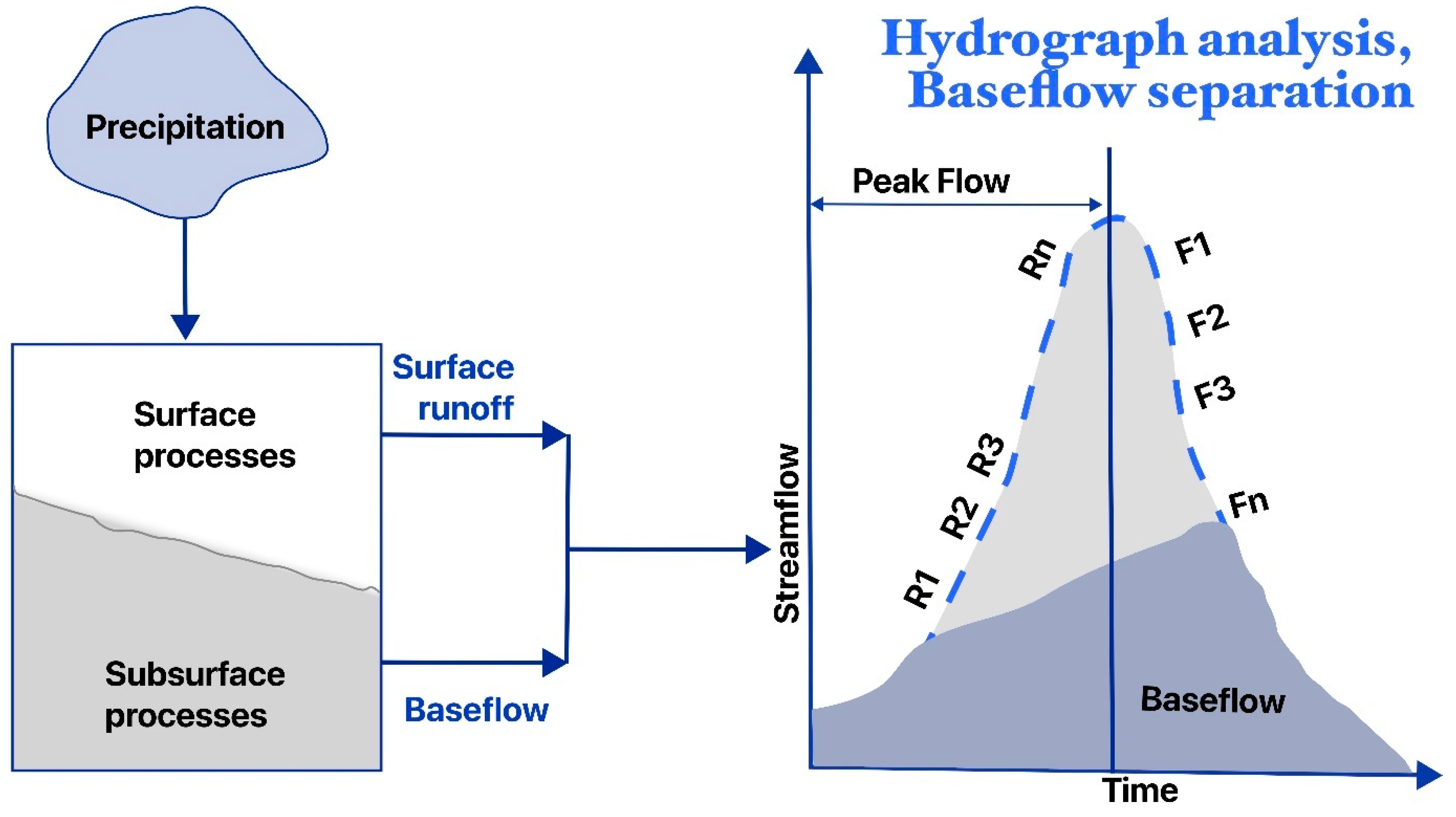
4.2. Hydrograph Separation and Analysis-Based Streamflow Prediction-Enhancing Techniques

Distinct watershed processes and weather conditions are recognized to generate streamflow differently under low-, medium-, and high-flow conditions. Hence, a universal data-driven model would not be effective in accurately predicting both high and low runoff occurrences [143]. One way to improve the performance of models that perform poorly during certain periods is to identify the dominant components of the model during those periods. In this regard, various techniques have been proposed, including partitioning streamflow into baseflow and runoff, flow pattern recognition, and hydrograph segmenting. By inputting this information into data-driven models, temporal details of physical processes can be integrated.

Recently, several studies have suggested the use of baseflow separation techniques to improve flow prediction [13,15,144]. Furthermore, data partitioning into low and high flow and detailed hydrograph segmentation have also been used to enhance accuracy in DDM (Table 2).

4.2.1. Baseflow Separation

Streamflow at a watershed outlet is the sum of surface and subsurface flows, assuming simplified hydrology (Figure 6). While surface runoff represents the watershed’s response to precipitation, ET, and other surface processes, baseflow is the gradual release of groundwater-sustained water from the subsurface [145]. Therefore, separating baseflow and incorporating it into data-driven models is considered a way to include flow domain knowledge.

Corzo and Solomatine [26] tested time-based (e.g., straight line) and process-based (e.g., recursive digital filter) baseflow separation techniques and found that even traditional semi-empirical methods such as constant slope can improve simulation accuracy. However, the model with an optimized baseflow filtering equation performed best. Other studies [15] support this conclusion. Zemzami and Benaabidate [15] showed that recursive digital filters outperformed one-parameter digital filters in improving the performance of ANN models. Although several baseflow separation techniques exist, one-parameter or recursive digital filters [146,147] are commonly used for improved flow prediction studies.

Two approaches have been used to improve SFP using baseflow separation techniques. The first approach uses baseflow as a predictor alongside other input variables [25,144,148]. The second approach builds separate models for baseflow and excess flow and then combines the results [26,56,149]. Various models, including ELM and LSTM, have been used to investigate the effectiveness of this technique in various regions [25,26,149]. However, there is no comparison study or clear argument for selecting one over the other despite both approaches improving SFP.

4.2.2. Identifying Flow Events

The independent use of low- and high-flow separation techniques has significantly improved flow simulation, in addition to their use in conjunction with baseflow separation techniques [26,56,150,151]. Cannas et al. [150] found that manually partitioning the data into low, medium, and high flows produced better results than preprocessing the data using signal-processing algorithms. Moreover, recent studies used simple methods to identify dry and wet periods and found improved model performance. Araghinejad et al. [151] built different ANN models for dry and wet conditions. To add more physical consistency, Xie et al. [14] introduced physical mechanisms such as simple water balance to identify extreme events and a monotonic relationship identification method to improve extreme event prediction in the LSTM model.

4.2.3. Hydrograph Segmenting

Hydrological studies typically divide streamflow into baseflow and excess flow, but streamflow generation is a complex process involving multiple stages, including the ascending and descending limbs of a hydrograph and its baseflow [152,153]. The distinct segments of a flow hydrograph are generated by a range of physical watershed mechanisms [154]. Moreover, each portion of the hydrograph has a different relationship with weather properties. For example, baseflow has a higher relation with soil moisture content and groundwater discharge than precipitation.

Jain and Srinivasulu [154] showed that a hydrograph segmenting-based ANN model outperformed a model for the entire hydrograph. They developed five models: (1) a benchmark model for the entire hydrograph, (2) a model for the rising and falling limbs, (3) a model for the rising limb with recession analysis applied to the falling limb, and (4) a model that splits the falling limb into two sections based on surface flow and interflow dominance. Srinivasulu and Jain [145] used an ANN and elitist real-coded genetic algorithm (ERGA) with hydrograph segmentation, dividing the hydrograph into four segments, two on each rising and falling limb. Recently, Li et al. [155] proposed five flow pattern classes: monotonic rising, monotonic falling, monotonic stable, concave, and convex. They used pattern recognition to build ANN and SVM models. Furthermore, Shen et al. [153] segmented a hydrograph into baseflow, rising limb, and falling limb using the self-organizing map (SOM) and then grouped the hydro-meteorological data accordingly to improve flow prediction.

Table 2. Overview of the reviewed works that couple hydrograph analysis and baseflow separation with data-driven models to enhance prediction accuracy.

Methods	Input Variables	Study Region	Data-Driven Models	Authors	Finding/Remark
Data portioning into three groups based on low-, medium-, and high-flow events	Rainfall, temperature	USA	ANN	[11]	Satisfactory result for average event; unsatisfactory result for extreme events.
Hydrograph decomposition, recession analysis	Effective rainfall, streamflow	USA	ANN	[154]	Decomposing a flow hydrograph enhanced prediction more effectively than preprocessing with a self-organizing map.
Data portioning into low, medium, and high	Streamflow	Italy	ANN	[150]	Basic data partitioning yielded better predictions than models based on signal-processed data.
Clustering into low and high flow, time-based and recursive baseflow separation	Precipitation, streamflow	Nepal, Italy, U.K.	ANN, modular approach	[26]	Hydrology-informed ANNs surpassed standard ANNs.
Baseflow separation	Precipitation, streamflow	Nepal, Italy	ANN, modular approach	[156]	Domain knowledge made the ANN more accurate.
Hydrograph decomposed into four: two in each rising and falling limb	Rainfall, streamflow	USA	ANN, ERGA	[145]	The approach yielded more accurate predictions than the conceptual model that was used.
Baseflow separation (Bflow), decomposing into low and high flow	Precipitation, ET, infiltration depth, surface runoff	USA	ANN, modular approach	[56]	Management scenario assessment.
Recursive baseflow separation	Climate, streamflow	USA	ELM, modular approach	[149]	The modular model did not enhance SFP.
Baseflow separation (one-parameter digital filter and recursive digital filter)	Precipitation, streamflow	Morocco	ANN	[15]	Improved peak flow was found. The ANN using baseflow performed better than the signal processed-based model.
Separating low and high flow	Streamflow	Iran	ANN	[151]	Enhanced high and low flow prediction were achieved.
Recursive baseflow separation	Climate, PET, streamflow	USA	SVR, ANN, RF	[144]	Baseflow separation enhanced streamflow simulation accuracy.
Baseflow separation using the Lyne–Hollick method	Streamflow	China	ANN, LSTM, SVM, Holt–Winter, GRU, ARIMA	[148]	The model prediction performance improved.
Flow pattern recognition (five classes)	Streamflow	China	ANN, SVM	[155]	Models with flow classes outperformed the other models.
Extreme events and monotonic rainfall–runoff relationshiop	Climate data	USA	LSTM	[14]	Model performance improved compared with LSTM.
Clustering flow: baseflow, rising limb, falling limb	Rainfall, evaporation, surface soil moisture, streamflow	China	Deep Belief Networks (DBNs)	[153]	Improved peak values and higher accuracy.
Process-based baseflow separation	Climate, irrigation, streamflow	China	Stepwise cluster	[13]	The hybrid model outperformed the conventional data-driven models.
One-parameter recursive single-pass filter baseflow separation method	Climate, PET, streamflow	USA	ANN, LSTM	[25]	Improved low-flow prediction.

Table 2. Overview of the reviewed works that couple hydrograph analysis and baseflow separation with data-driven models to enhance prediction accuracy.

Methods	Input Variables	Study Region	Data-Driven Models	Authors	Finding/Remark
Data portioning into three groups based on low-, medium-, and high-flow events	Rainfall, temperature	USA	ANN	[11]	Satisfactory result for average event; unsatisfactory result for extreme events.
Hydrograph decomposition, recession analysis	Effective rainfall, streamflow	USA	ANN	[154]	Decomposing a flow hydrograph enhanced prediction more effectively than preprocessing with a self-organizing map.
Data portioning into low, medium, and high	Streamflow	Italy	ANN	[150]	Basic data partitioning yielded better predictions than models based on signal-processed data.
Clustering into low and high flow, time-based and recursive baseflow separation	Precipitation, streamflow	Nepal, Italy, U.K.	ANN, modular approach	[26]	Hydrology-informed ANNs surpassed standard ANNs.
Baseflow separation	Precipitation, streamflow	Nepal, Italy	ANN, modular approach	[156]	Domain knowledge made the ANN more accurate.
Hydrograph decomposed into four: two in each rising and falling limb	Rainfall, streamflow	USA	ANN, ERGA	[145]	The approach yielded more accurate predictions than the conceptual model that was used.
Baseflow separation (Bflow), decomposing into low and high flow	Precipitation, ET, infiltration depth, surface runoff	USA	ANN, modular approach	[56]	Management scenario assessment.
Recursive baseflow separation	Climate, streamflow	USA	ELM, modular approach	[149]	The modular model did not enhance SFP.
Baseflow separation (one-parameter digital filter and recursive digital filter)	Precipitation, streamflow	Morocco	ANN	[15]	Improved peak flow was found. The ANN using baseflow performed better than the signal processed-based model.
Separating low and high flow	Streamflow	Iran	ANN	[151]	Enhanced high and low flow prediction were achieved.
Recursive baseflow separation	Climate, PET, streamflow	USA	SVR, ANN, RF	[144]	Baseflow separation enhanced streamflow simulation accuracy.
Baseflow separation using the Lyne–Hollick method	Streamflow	China	ANN, LSTM, SVM, Holt–Winter, GRU, ARIMA	[148]	The model prediction performance improved.
Flow pattern recognition (five classes)	Streamflow	China	ANN, SVM	[155]	Models with flow classes outperformed the other models.
Extreme events and monotonic rainfall–runoff relationshiop	Climate data	USA	LSTM	[14]	Model performance improved compared with LSTM.
Clustering flow: baseflow, rising limb, falling limb	Rainfall, evaporation, surface soil moisture, streamflow	China	Deep Belief Networks (DBNs)	[153]	Improved peak values and higher accuracy.
Process-based baseflow separation	Climate, irrigation, streamflow	China	Stepwise cluster	[13]	The hybrid model outperformed the conventional data-driven models.
One-parameter recursive single-pass filter baseflow separation method	Climate, PET, streamflow	USA	ANN, LSTM	[25]	Improved low-flow prediction.

5. Discussion and Future Direction

For decades, DDM has been used alongside or in conjunction with PBM, sparking a debate about their relative effectiveness and potential for synergy. Kim et al. [16] challenged whether AI and DDMs could rival or surpass PBMs in streamflow simulation, while Nearing et al. [12] emphasized the crucial role of hydrological science in the age of machine learning, suggesting a future hydrology encompassing both PBMs and DDMs. This research area has expanded rapidly, embracing advanced deep learning and hybrid techniques. Efforts to incorporate hydrograph segmentation, baseflow analysis, and PBMs into DDMs aim to create physically consistent and interpretable models, addressing hydrologists’ concerns about the reliability of process-less models in dynamic environments [12,157,158]. PBM techniques are the most prevalent among the used methods (Figure 7a). Even the simplest output processing techniques have demonstrably enhanced prediction performance. Additionally, metaheuristic algorithms have been used for parameter optimization and input variable selection to further improve prediction accuracy [159]. HBV and SWAT are the most widely used hydrological models, along with various data-driven models (Figure 7b).

Each method has its limitations and advantages. Simulated flow as input offers low interpretability but can help with data scarcity. Introducing intermediate variables provides moderate interpretability and flexibility. Replacing modules allows for high interpretability and transparency. Baseflow separation and hydrograph segmenting offer moderate to high interpretability but require expertise in flow patterns and an understanding of the hydrograph.

5.1. Research Gap

In the realm of utilizing PBM outputs, it is important to acknowledge the widespread use of both calibrated and uncalibrated model outputs in various studies. Intriguingly, while specific research [118] underscores the superiority of calibrated model outputs, a body of evidence [94,140], suggests that both calibrated and uncalibrated PBM outputs can contribute to the enhancement of SFP. This situation raises a pertinent question: Should our priority lie in using calibrated models, or should we opt for uncalibrated ones? On a parallel note, the incorporation of PBM outputs like residual error and streamflow prompts a critical consideration: do these models primarily serve as tools for data production, or do they genuinely integrate hydrological science into DDM? Consequently, one must ponder whether the improved predictions maintain physical consistency.

Moreover, the variability in intermediate variables within different hydroclimatic regions and their impacts on the streamflow generation process introduce added complexities. Model performance can vary significantly across these hydroclimatic regions [141]. However, the effectiveness of the modeling framework may also depend on the efficiency of the process-based model module that is used. These lead to further questions, such as whether different baseflow separation techniques might yield varying effects on model predictions and whether model complexity and overfitting pose risks within the integrated modeling framework.

5.1.1. The Role of Hydrological Science

The integration of process-based and data-driven models has the potential to enhance the accuracy of hydrological process representation in data-driven models [12]. However, current research tends to lean heavily on using simulated streamflow or residual error as input for data-driven models rather than introducing a variety of hydrological processes from PBM. This approach may lead to hydrological process information being presented to data-driven models in a more generalized form, which could make the effort to improve the interpretability of the model outputs less effective. The integration of intermediate variables from PBM into DDM, as well as the replacement of selected process-based modules with data-driven models, has yet to be thoroughly explored.

While nearly all techniques reviewed in this paper demonstrate improved prediction performance, most, including those utilizing simulated outputs, still render the data-driven model as a “black box”. Therefore, alongside prediction accuracy, it is time to emphasize the role of hydrologic science within the integrated modeling framework.

5.1.2. Model Interpretability and Transferability

The main drawback of empirical hydrological models that rely solely on data is that they are typically only valid under the same conditions in which they were first developed [6]. Despite being a concern for hydrologists for several years, this issue remains unsolved and has not been adequately addressed, even with recent advancements. The robustness of both data-driven models and PBM in adapting to changing hydroclimatic conditions has been a challenge, with DDM proving to be less robust [160]. Most of the novel techniques proposed failed to show robustness in the changing environment.

Limited studies [81,106,139] discussed the practical aspect of enhanced prediction. Many studies fail to justify their selection of a specific technique over others. Instead, they repeatedly stress the importance of additional techniques to improve model performance, often solely motivated by the desire to achieve higher performance indices. However, even when comparative studies demonstrate the superiority of one technique over another, little attention is given to explaining the reasoning behind choosing one over the other and the practical aspect. As a result, there is a lack of transparency, which hinders the reproducibility and comparability of research findings.

Comparison among the commonly used methods is scarce. The efficacy of different approaches varies across a region [141]. Particularly, the selection of intermediate variables has a significant effect on streamflow generation processes and prediction accuracy in different regions.

5.1.3. Risk of Overfitting and Model Complexity

DDM has evolved significantly over time, transitioning from simplistic single-input models to the prevalent multivariate modeling approach. This shift has spurred a growing interest in integrating multiple models to enhance predictive accuracy. While this process appears robust, the increased complexity of modeling and the need for algorithm comprehension amplify the risk of overfitting and errors. A common practice of using PBM as a data production mechanism can inadvertently contribute to overfitting in DDM. Furthermore, the effective implementation of modeling processes demands expertise in various algorithms and toolboxes, as these tools are often scattered across different packages. Studies focusing on model complexity and overfitting warrant further attention to address these challenges and improve the overall robustness of DDM for physically consistent SFP.

5.2. Promising Areas for Future Research

After 2014, a surge in publications, particularly those focused on integrating PBM into the DDM framework (Figure 8), shows the growing concern for interpretability and physical consistency. Recently, several physics-informed algorithms and toolkits have emerged [125,134,158]. The development of various tools and physics-informed machine learning can be considered a promising area of research in SFP.

5.2.1. Emergence Physics-Wrapped Neural Networks

Using process-based models merely as data-generating tools limits their ability to provide feedback within the modeling framework [122,129,161]. Consequently, the integrated modeling framework remains less interpretable. In response to this limitation, physics-wrapped machine learning algorithms such as physics-informed neural networks (PINNs) and differentiable machine learning have emerged. These algorithms incorporate physics-based equations, typically in the form of differential equations, directly into their structure. These equations act as regularization agents during training, ensuring that the PINN parameters align with the embedded governing equations and enable accurate and efficient gradient computations with respect to model variables. Moreover, the fabric is flexible enough to incorporate expert knowledge or replace the required module [122,126,127,142].

5.2.2. Applicability in Ungauged Regions and Assessment of Natural and Anthropogenic Factors

Hydrological models typically require calibration and validation before they can be effectively used for management or forecasting. This task poses a challenge, especially in ungauged or poorly gauged watersheds. PBM approaches have addressed this challenge with parameter transfer techniques [123,162]. A similar approach is used in DDM [163]. Recently, the applicability of the physically consistent DDM approach in ungauged regions has been discussed in the literature. For instance, Chen et al. [139] initially trained an LSTM model using weather data and SWAT outputs (intermediate variables) from data-rich regions. They then applied transfer learning to ungauged watersheds. The resulting coupled model improved SFP but tended to underestimate peak flow during the simulation period. In another study, Feng et al. [142] investigated physics-informed, differentiable machine-learning hydrologic models for ungauged regions and climate change assessment. Their results demonstrated the superior performance of these models over LSTM in ungauged regions.

Assessing streamflow responses to management scenarios and climate change is a critical area of research. However, both process-based and data-driven models can produce unreliable predictions [126,137]. Given the importance of the ET module in evaluating climate change impacts, enhancing prediction accuracy could involve either replacing the ET module in process-based models or incorporating simulated ET into a DDM framework. For instance, Wi and Steinschneider [137] investigated the predictive abilities of process-based models and deep learning techniques in the context of climate change. They observed that while all process-based models exhibited decreased runoff ratios and seasonal shifts, LSTM models showed unrealistic increases in runoff ratios for certain watersheds. Notably, LSTM generated reasonable results when the SAC model-simulated ET was used as input. In another study, Zhong et al. [126] enhanced the EXP-HYDRO model by incorporating a P-RNN layer to assess climate change’s impact on streamflow. This physics-informed deep learning model excelled in simulating streamflow across different timescales, accounting for soil freeze–thaw effects, and capturing changes in runoff trends associated with climate change.

6. Summary and Outlook

Streamflow modeling is crucial for effective water management and risk assessment, encompassing tasks such as optimizing water allocation, assessing water quality, and predicting floods and droughts. Accurate SFP poses a challenge due to the intricate interplay between subsurface and surface processes. Traditional DDM and PBM approaches often fall short of accurately estimating or forecasting extreme events. To enhance SFP accuracy within a data-driven framework, various techniques, including advanced algorithms, have been proposed. While numerous review papers on data-driven hydrological modeling exist, there remains a need for a comprehensive and clear roadmap for improving SFP with physical consistency and domain knowledge. To address this gap, this paper offers a well-structured review of popular SFP-enhancing techniques in a physically consistent and domain knowledge approach.

The primary practices reviewed encompass PBM and hydrograph analysis. PBM approaches include simulated streamflow and intermediate variables, residual error-focused techniques, and replacing selected modules. Hydrograph-related practices include baseflow separation, simple hydrograph decomposition into low and high flow, and detailed hydrograph segmenting. These techniques are motivated by various factors, such as the nonlinear nature of streamflow due to different hydrological processes being responsible for different parts of the hydrograph and the need for model reliability. Others aspire to incorporate physical consistency and interpretability using a physics-informed approach and expert knowledge.

To evaluate the effectiveness of these techniques, researchers have compared their performance against that of traditional models. Notably, an increasing trend is evident toward integrating physically models with data-driven models and baseflow separation techniques, which have experienced a consistent rise in popularity. In particular, physics-warped algorithms such as physics-embedded neural networks and differentiable machine learning offer the flexibility to replace specific hydrological model modules and incorporate expert knowledge into the modeling framework. These approaches hold promise for enhancing SFP in a physically consistent manner. Despite these promising advancements, a concerning lack of attention exists regarding potential issues related to model complexity, overfitting, and robustness. This underscores the need for further research aimed at improving model interpretability and robustness while mitigating these challenges.

References

1. Gleeson, T.; Wang-Erlandsson, L.; Porkka, M.; Zipper, S.C.; Jaramillo, F.; Gerten, D.; Fetzer, I.; Cornell, S.E.; Piemontese, L.; Gordon, L.J.; et al. Illuminating Water Cycle Modifications and Earth System Resilience in the Anthropocene. Water Resour. Res. 2020, 56, e2019WR024957. [Google Scholar] [CrossRef]
2. Carlisle, D.M.; Wolock, D.M.; Meador, M.R. Alteration of Streamflow Magnitudes and Potential Ecological Consequences: A Multiregional Assessment. Front. Ecol. Environ. 2011, 9, 264–270. [Google Scholar] [CrossRef]
3. Quang, N.H.; Viet, T.Q.; Thang, H.N.; Hieu, N.T.D. Long-Term Water Level Dynamics in the Red River Basin in Response to Anthropogenic Activities and Climate Change. Sci. Total Environ. 2024, 912, 168985. [Google Scholar] [CrossRef] [PubMed]
4. Depetris, P.J. The Importance of Monitoring River Water Discharge. Front. Water 2021, 3, 745912. [Google Scholar] [CrossRef]
5. Al Sawaf, M.B.; Kawanisi, K. Assessment of Mountain River Streamflow Patterns and Flood Events Using Information and Complexity Measures. J. Hydrol. 2020, 590, 125508. [Google Scholar] [CrossRef]
6. Bourdin, D.R.; Fleming, S.W.; Stull, R.B. Streamflow Modelling: A Primer on Applications, Approaches and Challenges. Atmos.-Ocean 2012, 50, 507–536. [Google Scholar] [CrossRef]
7. Mai, J.; Craig, J.R.; Tolson, B.A.; Arsenault, R. The Sensitivity of Simulated Streamflow to Individual Hydrologic Processes across North America. Nat. Commun. 2022, 13, 455. [Google Scholar] [CrossRef]
8. Solomatine, D.P.; Ostfeld, A. Data-Driven Modelling: Some Past Experiences and New Approaches. J. Hydroinform. 2008, 10, 3–22. [Google Scholar] [CrossRef]
9. Devia, G.K.; Ganasri, B.P.; Dwarakish, G.S. A Review on Hydrological Models. Aquat. Procedia 2015, 4, 1001–1007. [Google Scholar] [CrossRef]
10. Yaseen, Z.M.; El-shafie, A.; Jaafar, O.; Afan, H.A.; Sayl, K.N. Artificial Intelligence Based Models for Stream-Flow Forecasting: 2000–2015. J. Hydrol. 2015, 530, 829–844. [Google Scholar] [CrossRef]
11. Zhang, B.; Govindaraju, R.S. Prediction of Watershed Runoff Using Bayesian Concepts and Modular Neural Networks. Water Resour. Res. 2000, 36, 753–762. [Google Scholar] [CrossRef]
12. Nearing, G.S.; Kratzert, F.; Sampson, A.K.; Pelissier, C.S.; Klotz, D.; Frame, J.M.; Prieto, C.; Gupta, H.V. What Role Does Hydrological Science Play in the Age of Machine Learning? Water Resour. Res. 2021, 57, e2020WR028091. [Google Scholar] [CrossRef]
13. Li, K.; Huang, G.; Wang, S.; Razavi, S. Development of a Physics-Informed Data-Driven Model for Gaining Insights into Hydrological Processes in Irrigated Watersheds. J. Hydrol. 2022, 613, 128323. [Google Scholar] [CrossRef]
14. Xie, K.; Liu, P.; Zhang, J.; Han, D.; Wang, G.; Shen, C. Physics-Guided Deep Learning for Rainfall-Runoff Modeling by Considering Extreme Events and Monotonic Relationships. J. Hydrol. 2021, 603, 127043. [Google Scholar] [CrossRef]
15. Zemzami, M.; Benaabidate, L. Improvement of Artificial Neural Networks to Predict Daily Streamflow in a Semi-Arid Area. Hydrol. Sci. J. 2016, 61, 1801–1812. [Google Scholar] [CrossRef]
16. Kim, T.; Yang, T.; Gao, S.; Zhang, L.; Ding, Z.; Wen, X.; Gourley, J.J.; Hong, Y. Can Artificial Intelligence and Data-Driven Machine Learning Models Match or Even Replace Process-Driven Hydrologic Models for Streamflow Simulation?: A Case Study of Four Watersheds with Different Hydro-Climatic Regions across the CONUS Daily Streamflow. J. Hydrol. 2021, 598, 126423. [Google Scholar] [CrossRef]
17. Dawson, C.W.; Wilby, R.L. Hydrological Modelling Using Artificial Neural Networks. Prog. Phys. Geogr. 2001, 25, 80–108. [Google Scholar] [CrossRef]
18. Abrahart, R.J.; Anctil, F.; Coulibaly, P.; Dawson, C.W.; Mount, N.J.; See, L.M.; Shamseldin, A.Y.; Solomatine, D.P.; Toth, E.; Wilby, R.L. Two Decades of Anarchy? Emerging Themes and Outstanding Challenges for Neural Network River Forecasting. Prog. Phys. Geogr. Earth Environ. 2012, 36, 480–513. [Google Scholar] [CrossRef]
19. Boucher, M.-A.; Quilty, J.; Adamowski, J. Data Assimilation for Streamflow Forecasting Using Extreme Learning Machines and Multilayer Perceptrons. Water Resour. Res. 2020, 56, e2019WR026226. [Google Scholar] [CrossRef]
20. Cho, K.; Kim, Y. Improving Streamflow Prediction in the WRF-Hydro Model with LSTM Networks. J. Hydrol. 2022, 605, 127297. [Google Scholar] [CrossRef]
21. Lu, D.; Konapala, G.; Painter, S.L.; Kao, S.-C.; Gangrade, S. Streamflow Simulation in Data-Scarce Basins Using Bayesian and Physics-Informed Machine Learning Models. J. Hydrometeorol. 2021, 22, 1421–1438. [Google Scholar] [CrossRef]
22. Brunner, M.I.; Slater, L.; Tallaksen, L.M.; Clark, M. Challenges in Modeling and Predicting Floods and Droughts: A Review. WIREs Water 2021, 8, e1520. [Google Scholar] [CrossRef]
23. Bailey, R.T.; Wible, T.C.; Arabi, M.; Records, R.M.; Ditty, J. Assessing Regional-Scale Spatio-Temporal Patterns of Groundwater-Surface Water Interactions Using a Coupled SWAT-MODFLOW Model. Hydrol. Process. 2016, 143, 103662. [Google Scholar] [CrossRef]
24. El Hassan, A.A.; Sharif, H.O.; Jackson, T.; Chintalapudi, S. Performance of a Conceptual and Physically Based Model in Simulating the Response of a Semi-urbanized Watershed in San Antonio, Texas. Hydrol. Process. 2013, 27, 3394–3408. [Google Scholar] [CrossRef]
25. Tongal, H.; Booij, M.J. Simulated Annealing Coupled with a Naïve Bayes Model and Base Flow Separation for Streamflow Simulation in a Snow Dominated Basin. Stoch. Environ. Res. Risk Assess. 2022, 37, 89–112. [Google Scholar] [CrossRef]
26. Corzo, G.; Solomatine, D. Baseflow Separation Techniques for Modular Artificial Neural Network Modelling in Flow Forecasting. Hydrol. Sci. J. 2007, 52, 491–507. [Google Scholar] [CrossRef]
27. Nourani, V.; Hosseini Baghanam, A.; Adamowski, J.; Kisi, O. Applications of Hybrid Wavelet–Artificial Intelligence Models in Hydrology: A Review. J. Hydrol. 2014, 514, 358–377. [Google Scholar] [CrossRef]
28. Ibrahim, K.S.M.H.; Huang, Y.F.; Ahmed, A.N.; Koo, C.H.; El-Shafie, A. A Review of the Hybrid Artificial Intelligence and Optimization Modelling of Hydrological Streamflow Forecasting. Alex. Eng. J. 2022, 61, 279–303. [Google Scholar] [CrossRef]
29. Zounemat-Kermani, M.; Batelaan, O.; Fadaee, M.; Hinkelmann, R. Ensemble Machine Learning Paradigms in Hydrology: A Review. J. Hydrol. 2021, 598, 126266. [Google Scholar] [CrossRef]
30. Papacharalampous, G.; Tyralis, H. A Review of Machine Learning Concepts and Methods for Addressing Challenges in Probabilistic Hydrological Post-Processing and Forecasting. Front. Water 2022, 4, 166. [Google Scholar] [CrossRef]
31. Ng, K.W.; Huang, Y.F.; Koo, C.H.; Chong, K.L.; El-Shafie, A.; Najah Ahmed, A. A Review of Hybrid Deep Learning Applications for Streamflow Forecasting. J. Hydrol. 2023, 625, 130141. [Google Scholar] [CrossRef]
32. Mohammadi, B.; Safari, M.J.S.; Vazifehkhah, S. IHACRES, GR4J and MISD-Based Multi Conceptual-Machine Learning Approach for Rainfall-Runoff Modeling. Sci. Rep. 2022, 12, 12096. [Google Scholar] [CrossRef] [PubMed]
33. Beven, K. Rainfall-Runoff Modelling, 2nd ed.; Wiley: Chichester, UK, 2012; ISBN 9780470714591. [Google Scholar]
34. Seibert, J.; Vis, M.J.P. Teaching Hydrological Modeling with a User-Friendly Catchment-Runoff-Model Software Package. Hydrol. Earth Syst. Sci. 2012, 16, 3315–3325. [Google Scholar] [CrossRef]
35. Perrin, C.; Michel, C.; Andréassian, V. Improvement of a Parsimonious Model for Streamflow Simulation. J. Hydrol. 2003, 279, 275–289. [Google Scholar] [CrossRef]
36. Liang, X.; Lettenmaier, D.P.; Wood, E.F.; Burges, S.J. A Simple Hydrologically Based Model of Land Surface Water and Energy Fluxes for General Circulation Models. J. Geophys. Res. 1994, 99, 14415. [Google Scholar] [CrossRef]
37. Hydrologic Engineering Center. Hydrologic Engineering Center. Hydrologic Modeling System Technical Reference Manual. In Hydrologic Modeling System HEC-HMS: Technical Reference Manual; Hydrologic Engineering Center: Davis, CA, USA, 2000; p. 148. [Google Scholar]
38. Regan, R.S.; Markstrom, S.L.; Hay, L.E.; Viger, R.J.; Norton, P.A.; Driscoll, J.M.; Lafontaine, J.H. Description of the National Hydrologic Model for Use with the Precipitation-Runoff Modeling System (PRMS); U.S. Geological Survey: Reston, VA, USA, 2018.
39. Arnold, J.G.; Srinivasan, R.; Muttiah, R.S.; Williams, J.R. Large Area Hydrologic Modeling and Assessment Part I: Model Development. J. Am. Water Resour. Assoc. 1998, 34, 73–89. [Google Scholar] [CrossRef]
40. Victor Mockus. SCS National Engineering Handbook, Section 4: Hydrology; TheService: Washington, DC, USA, 1965; p. 127. ISBN NTIS #PB87101580. Available online: https://www.irrigationtoolbox.com/NEH/Part630Hydrology/neh630-ch21.pdf (accessed on 2 January 2024).
41. Monteith, J.L. Evaporation and Environment. In Proceedings of the Symposia of the Society for Experimental Biology; Volume 19, pp. 205–234. Available online: https://repository.rothamsted.ac.uk/item/8v5v7 (accessed on 2 January 2024).
42. Hargreaves, G.H.; Samani, Z.A. Samani Reference Crop Evapotranspiration from Temperature. Appl. Eng. Agric. 1985, 1, 96–99. [Google Scholar] [CrossRef]
43. Solomatine, D.; See, L.M.; Abrahart, R.J. Data-Driven Modelling: Concepts, Approaches and Experiences. In Practical Hydroinformatics; Springer: Berlin/Heidelberg, Germany, 2008; pp. 17–30. [Google Scholar]
44. Zhang, Z.; Zhang, Q.; Singh, V.P. Univariate Streamflow Forecasting Using Commonly Used Data-Driven Models: Literature Review and Case Study. Hydrol. Sci. J. 2018, 63, 1091–1111. [Google Scholar] [CrossRef]
45. Zounemat-Kermani, M.; Matta, E.; Cominola, A.; Xia, X.; Zhang, Q.; Liang, Q.; Hinkelmann, R. Neurocomputing in Surface Water Hydrology and Hydraulics: A Review of Two Decades Retrospective, Current Status and Future Prospects. J. Hydrol. 2020, 588, 125085. [Google Scholar] [CrossRef]
46. Sudheer, K.P.; Nayak, P.C.; Ramasastri, K.S. Improving Peak Flow Estimates in Artificial Neural Network River Flow Models. Hydrol. Process. 2003, 17, 677–686. [Google Scholar] [CrossRef]
47. Maier, H.R.; Jain, A.; Dandy, G.C.; Sudheer, K.P. Methods Used for the Development of Neural Networks for the Prediction of Water Resource Variables in River Systems: Current Status and Future Directions. Environ. Model. Softw. 2010, 25, 891–909. [Google Scholar] [CrossRef]
48. Taormina, R.; Galelli, S.; Karakaya, G.; Ahipasaoglu, S.D. An Information Theoretic Approach to Select Alternate Subsets of Predictors for Data-Driven Hydrological Models. J. Hydrol. 2016, 542, 18–34. [Google Scholar] [CrossRef]
49. Zheng, F.; Maier, H.R.; Wu, W.; Dandy, G.C.; Gupta, H.V.; Zhang, T. On Lack of Robustness in Hydrological Model Development Due to Absence of Guidelines for Selecting Calibration and Evaluation Data: Demonstration for Data-Driven Models. Water Resour. Res. 2018, 54, 1013–1030. [Google Scholar] [CrossRef]
50. Wu, W.; May, R.J.; Maier, H.R.; Dandy, G.C. A Benchmarking Approach for Comparing Data Splitting Methods for Modeling Water Resources Parameters Using Artificial Neural Networks. Water Resour. Res. 2013, 49, 7598–7614. [Google Scholar] [CrossRef]
51. Reis, G.B.; da Silva, D.D.; Fernandes Filho, E.I.; Moreira, M.C.; Veloso, G.V.; Fraga, M.d.S.; Pinheiro, S.A.R. Effect of Environmental Covariable Selection in the Hydrological Modeling Using Machine Learning Models to Predict Daily Streamflow. J. Environ. Manag. 2021, 290, 112625. [Google Scholar] [CrossRef] [PubMed]
52. Galelli, S.; Castelletti, A. Tree-Based Iterative Input Variable Selection for Hydrological Modeling. Water Resour. Res. 2013, 49, 4295–4310. [Google Scholar] [CrossRef]
53. Taormina, R.; Chau, K.W. Data-Driven Input Variable Selection for Rainfall-Runoff Modeling Using Binary-Coded Particle Swarm Optimization and Extreme Learning Machines. J. Hydrol. 2015, 529, 1617–1632. [Google Scholar] [CrossRef]
54. May, R.J.; Maier, H.R.; Dandy, G.C.; Fernando, T.M.K.G. Non-Linear Variable Selection for Artificial Neural Networks Using Partial Mutual Information. Environ. Model. Softw. 2008, 23, 1312–1326. [Google Scholar] [CrossRef]
55. Sola, J.; Sevilla, J. Importance of Input Data Normalization for the Application of Neural Networks to Complex Industrial Problems. IEEE Trans. Nucl. Sci. 1997, 44, 1464–1468. [Google Scholar] [CrossRef]
56. Isik, S.; Kalin, L.; Schoonover, J.E.; Srivastava, P.; Graeme Lockaby, B. Modeling Effects of Changing Land Use/Cover on Daily Streamflow: An Artificial Neural Network and Curve Number Based Hybrid Approach. J. Hydrol. 2013, 485, 103–112. [Google Scholar] [CrossRef]
57. Nourani, V.; Baghanam, A.H.; Adamowski, J.; Gebremichael, M. Using Self-Organizing Maps and Wavelet Transforms for Space–Time Pre-Processing of Satellite Precipitation and Runoff Data in Neural Network Based Rainfall–Runoff Modeling. J. Hydrol. 2013, 476, 228–243. [Google Scholar] [CrossRef]
58. Teegavarapu, R.S.V.; Sharma, P.J.; Lal Patel, P. Frequency-Based Performance Measure for Hydrologic Model Evaluation. J. Hydrol. 2022, 608, 127583. [Google Scholar] [CrossRef]
59. Nash, J.E.E.; Sutcliffe, J.V. River Flow Forecasting through Conceptual Models Part I—A Discussion of Principles. J. Hydrol. 1970, 10, 282–290. [Google Scholar] [CrossRef]
60. Hwang, S.H.; Ham, D.H.; Kim, J.H. A New Measure for Assessing the Efficiency of Hydrological Data-Driven Forecasting Models. Hydrol. Sci. J. 2012, 57, 1257–1274. [Google Scholar] [CrossRef]
61. Frame, J.M.; Kratzert, F.; Raney, A.; Rahman, M.; Salas, F.R.; Nearing, G.S. Post-Processing the National Water Model with Long Short-Term Memory Networks for Streamflow Predictions and Model Diagnostics. JAWRA J. Am. Water Resour. Assoc. 2021, 57, 885–905. [Google Scholar] [CrossRef]
62. Duan, Y.; Akula, S.; Kumar, S.; Lee, W.; Khajehei, S. A Hybrid Physics—AI Model to Improve Hydrological Forecasts. Artif. Intell. Earth Syst. 2023, 2, e220023. [Google Scholar] [CrossRef]
63. SugaWara, M. Automatic Calibration of the Tank Model. Hydrol. Sci. Bull. 1979, 24, 375–388. [Google Scholar] [CrossRef]
64. Brocca, L.; Melone, F.; Moramarco, T. Distributed Rainfall-Runoff Modelling for Flood Frequency Estimation and Flood Forecasting. Hydrol. Process. 2011, 25, 2801–2813. [Google Scholar] [CrossRef]
65. Tan, B.Q.; O’Connor, K.M. Application of an Empirical Infiltration Equation in the SMAR Conceptual Model. J. Hydrol. 1996, 185, 275–295. [Google Scholar] [CrossRef]
66. Lévite, H.; Sally, H.; Cour, J. Testing Water Demand Management Scenarios in a Water-Stressed Basin in South Africa: Application of the WEAP Model. Phys. Chem. Earth Parts A/B/C 2003, 28, 779–786. [Google Scholar] [CrossRef]
67. Crawford, N.H.; Thurin, S.M. Hydrologic Estimates for Small Hydroelectric Projects; Small Decentralized Hydropower Program; International Programs Division, National Rural Electric Cooperative Association: Arlington, TX, USA, 1981.
68. Yang, S.; Yang, D.; Chen, J.; Santisirisomboon, J.; Lu, W.; Zhao, B. A Physical Process and Machine Learning Combined Hydrological Model for Daily Streamflow Simulations of Large Watersheds with Limited Observation Data. J. Hydrol. 2020, 590, 125206. [Google Scholar] [CrossRef]
69. Yang, D.; Herath, S.; Musiake, K. Development of a Geomorphology-Based Hydrological Model for Large Catchments. Proc. Hydraul. Eng. 1998, 42, 169–174. [Google Scholar] [CrossRef]
70. Chiew, F.H.S.; Peel, M.C.; Western, A.W.; Singh, V.P.; Frevert, D.K. Mathematical Models of Small Watershed Hydrology and Applications; Water Resources Publication: Littleton, CO, USA, 2002; pp. 335–367. [Google Scholar]
71. Jakeman, A.J.; Littlewood, I.G.; Whitehead, P.G. Computation of the Instantaneous Unit Hydrograph and Identifiable Component Flows with Application to Two Small Upland Catchments. J. Hydrol. 1990, 117, 275–300. [Google Scholar] [CrossRef]
72. Quan, Z.; Teng, J.; Sun, W.; Cheng, T.; Zhang, J. Evaluation of the HYMOD Model for Rainfall–Runoff Simulation Using the GLUE Method. Proc. Int. Assoc. Hydrol. Sci. 2015, 368, 180–185. [Google Scholar] [CrossRef]
73. Burnash, R.J.C. The NWS River Forecast System-Catchment Modeling. In Computer Models of Watershed Hydrology; CAB International: Wallingford, UK, 1995; pp. 311–366. [Google Scholar]
74. Mouelhi, S.; Michel, C.; Perrin, C.; Andréassian, V. Stepwise Development of a Two-Parameter Monthly Water Balance Model. J. Hydrol. 2006, 318, 200–214. [Google Scholar] [CrossRef]
75. Jain, A.; Srinivasulu, S. Development of Effective and Efficient Rainfall-Runoff Models Using Integration of Deterministic, Real-Coded Genetic Algorithms and Artificial Neural Network Techniques. Water Resour. Res. 2004, 40, e2003WR002355. [Google Scholar] [CrossRef]
76. Noori, N.; Kalin, L. Coupling SWAT and ANN Models for Enhanced Daily Streamflow Prediction. J. Hydrol. 2016, 533, 141–151. [Google Scholar] [CrossRef]
77. Humphrey, G.B.; Gibbs, M.S.; Dandy, G.C.; Maier, H.R. A Hybrid Approach to Monthly Streamflow Forecasting: Integrating Hydrological Model Outputs into a Bayesian Artificial Neural Network. J. Hydrol. 2016, 540, 623–640. [Google Scholar] [CrossRef]
78. Ren, W.W.; Yang, T.; Huang, C.S.; Xu, C.Y.; Shao, Q.X. Improving Monthly Streamflow Prediction in Alpine Regions: Integrating HBV Model with Bayesian Neural Network. Stoch. Environ. Res. Risk Assess. 2018, 32, 3381–3396. [Google Scholar] [CrossRef]
79. Bhasme, P.; Vagadiya, J.; Bhatia, U. Enhancing Predictive Skills in Physically-Consistent Way: Physics Informed Machine Learning for Hydrological Processes. J. Hydrol. 2022, 615, 128618. [Google Scholar] [CrossRef]
80. Thomas, H.A. Improved Methods for National Water Assessment, Water Resources Contract: WR15249270; US Water Resources Council: Washington, DC, USA, 1981. [Google Scholar]
81. Xu, T.; Longyang, Q.; Tyson, C.; Zeng, R.; Neilson, B.T. Hybrid Physically Based and Deep Learning Modeling of a Snow Dominated, Mountainous, Karst Watershed. Water Resour. Res. 2022, 58, e2021WR030993. [Google Scholar] [CrossRef]
82. Mahat, V.; Tarboton, D.G. Representation of Canopy Snow Interception, Unloading and Melt in a Parsimonious Snowmelt Model. Hydrol. Process. 2014, 28, 6320–6336. [Google Scholar] [CrossRef]
83. Farfán, J.F.; Palacios, K.; Ulloa, J.; Avilés, A. A Hybrid Neural Network-Based Technique to Improve the Flow Forecasting of Physical and Data-Driven Models: Methodology and Case Studies in Andean Watersheds. J. Hydrol. Reg. Stud. 2020, 27, 100652. [Google Scholar] [CrossRef]
84. Mohammadi, B.; Moazenzadeh, R.; Christian, K.; Duan, Z. Improving Streamflow Simulation by Combining Hydrological Process-Driven and Artificial Intelligence-Based Models. Environ. Sci. Pollut. Res. 2021, 28, 65752–65768. [Google Scholar] [CrossRef]
85. Sikorska-Senoner, A.E.; Quilty, J.M. A Novel Ensemble-Based Conceptual-Data-Driven Approach for Improved Streamflow Simulations. Environ. Model. Softw. 2021, 143, 105094. [Google Scholar] [CrossRef]
86. Li, M.; Wang, Q.J.; Robertson, D.E.; Bennett, J.C. Improved Error Modelling for Streamflow Forecasting at Hourly Time Steps by Splitting Hydrographs into Rising and Falling Limbs. J. Hydrol. 2017, 555, 586–599. [Google Scholar] [CrossRef]
87. Li, D.; Marshall, L.; Liang, Z.; Sharma, A.; Zhou, Y. Characterizing Distributed Hydrological Model Residual Errors Using a Probabilistic Long Short-Term Memory Network. J. Hydrol. 2021, 603, 126888. [Google Scholar] [CrossRef]
88. Anctil, F.; Perrin, C.; Andréassian, V. ANN Output Updating of Lumped Conceptual Rainfall/Runoff Forecasting Models. J. Am. Water Resour. Assoc. 2003, 39, 1269–1279. [Google Scholar] [CrossRef]
89. Smith, T.; Marshall, L.; Sharma, A. Modeling Residual Hydrologic Errors with Bayesian Inference. J. Hydrol. 2015, 528, 29–37. [Google Scholar] [CrossRef]
90. Tian, Y.; Xu, Y.P.; Yang, Z.; Wang, G.; Zhu, Q. Integration of a Parsimonious Hydrological Model with Recurrent Neural Networks for Improved Streamflow Forecasting. Water 2018, 10, 1655. [Google Scholar] [CrossRef]
91. Han, H.; Morrison, R.R. Improved Runoff Forecasting Performance through Error Predictions Using a Deep-Learning Approach. J. Hydrol. 2022, 608, 127653. [Google Scholar] [CrossRef]
92. Yang, C.; Xu, M.; Kang, S.; Fu, C.; Hu, D. Improvement of Streamflow Simulation by Combining Physically Hydrological Model with Deep Learning Methods in Data-Scarce Glacial River Basin. J. Hydrol. 2023, 625, 129990. [Google Scholar] [CrossRef]
93. Kassem, A.A.; Raheem, A.M.; Khidir, K.M.; Alkattan, M. Predicting of Daily Khazir Basin Flow Using SWAT and Hybrid SWAT-ANN Models. Ain Shams Eng. J. 2020, 11, 435–443. [Google Scholar] [CrossRef]
94. Shen, Y.; Ruijsch, J.; Lu, M.; Sutanudjaja, E.H.; Karssenberg, D. Random Forests-Based Error-Correction of Streamflow from a Large-Scale Hydrological Model: Using Model State Variables to Estimate Error Terms. Comput. Geosci. 2022, 159, 105019. [Google Scholar] [CrossRef]
95. Roy, A.; Kasiviswanathan, K.S.; Patidar, S.; Adeloye, A.J.; Soundharajan, B.S.; Ojha, C.S.P. A Novel Physics-Aware Machine Learning-Based Dynamic Error Correction Model for Improving Streamflow Forecast Accuracy. Water Resour. Res. 2023, 59, e2022WR033318. [Google Scholar] [CrossRef]
96. Roy, A.; Kasiviswanathan, K.S.; Patidar, S.; Adeloye, A.J.; Soundharajan, B.; Ojha, C.S.P. A Physics-Aware Machine Learning-Based Framework for Minimizing Prediction Uncertainty of Hydrological Models. Water Resour. Res. 2023, 59, e2023WR034630. [Google Scholar] [CrossRef]
97. Young, C.-C.C.; Liu, W.-C.C.; Wu, M.-C.C. A Physically Based and Machine Learning Hybrid Approach for Accurate Rainfall-Runoff Modeling during Extreme Typhoon Events. Appl. Soft Comput. 2017, 53, 205–216. [Google Scholar] [CrossRef]
98. Kurian, C.; Sudheer, K.P.; Vema, V.K.; Sahoo, D. Effective Flood Forecasting at Higher Lead Times through Hybrid Modelling Framework. J. Hydrol. 2020, 587, 124945. [Google Scholar] [CrossRef]
99. Ghaith, M.; Siam, A.; Li, Z.; El-Dakhakhni, W. Hybrid Hydrological Data-Driven Approach for Daily Streamflow Forecasting. J. Hydrol. Eng. 2020, 25, 04019063. [Google Scholar] [CrossRef]
100. Chen, J.; Adams, B.J. Integration of Artificial Neural Networks with Conceptual Models in Rainfall-Runoff Modeling. J. Hydrol. 2006, 318, 232–249. [Google Scholar] [CrossRef]
101. Song, X.; Kong, F.; Zhan, C.; Han, J. Hybrid Optimization Rainfall-Runoff Simulation Based on Xinanjiang Model and Artificial Neural Network. J. Hydrol. Eng. 2012, 17, 1033–1041. [Google Scholar] [CrossRef]
102. Vidyarthi, V.K.; Jain, A. Incorporating Non-Uniformity and Non-Linearity of Hydrologic and Catchment Characteristics in Rainfall–Runoff Modeling Using Conceptual, Data-Driven, and Hybrid Techniques. J. Hydroinform. 2022, 24, 350–366. [Google Scholar] [CrossRef]
103. Ren-Jun, Z. The Xinanjiang Model Applied in China. J. Hydrol. 1992, 135, 371–381. [Google Scholar] [CrossRef]
104. Liu, S.; Xu, J.; Zhao, J.; Xie, X.; Zhang, W. Efficiency Enhancement of a Process-Based Rainfall–Runoff Model Using a New Modified AdaBoost.RT Technique. Appl. Soft Comput. 2014, 23, 521–529. [Google Scholar] [CrossRef]
105. Beven, K.J.; Kirkby, M.J. A Physically Based, Variable Contributing Area Model of Basin Hydrology. Hydrol. Sci. Bull. 1979, 24, 43–69. [Google Scholar] [CrossRef]
106. Mekonnen, B.A.; Nazemi, A.; Mazurek, K.A.; Elshorbagy, A.; Putz, G. Hybrid Modelling Approach to Prairie Hydrology: Fusing Data-Driven and Process-Based Hydrological Models. Hydrol. Sci. J. 2015, 60, 1473–1489. [Google Scholar] [CrossRef]
107. Liu, B.; Tang, Q.; Zhao, G.; Gao, L.; Shen, C.; Pan, B. Physics-Guided Long Short-Term Memory Network for Streamflow and Flood Simulations in the Lancang–Mekong River Basin. Water 2022, 14, 1429. [Google Scholar] [CrossRef]
108. Yamazaki, D.; Kanae, S.; Kim, H.; Oki, T. A Physically Based Description of Floodplain Inundation Dynamics in a Global River Routing Model. Water Resour. Res. 2011, 47, e2010WR009726. [Google Scholar] [CrossRef]
109. Zhou, Y.; Cui, Z.; Lin, K.; Sheng, S.; Chen, H.; Guo, S.; Xu, C.Y. Short-Term Flood Probability Density Forecasting Using a Conceptual Hydrological Model with Machine Learning Techniques. J. Hydrol. 2022, 604, 127255. [Google Scholar] [CrossRef]
110. Thalli Mani, S.; Kolluru, V.; Amai, M.; Acharya, T.D. Enhanced Streamflow Simulations Using Nudging Based Optimization Coupled with Data-Driven and Hydrological Models. J. Hydrol. Reg. Stud. 2022, 43, 101190. [Google Scholar] [CrossRef]
111. Li, Z.; Yu, J.; Xu, X.; Sun, W.; Pang, B.; Yue, J. Multi-Model Ensemble Hydrological Simulation Using a BP Neural Network for the Upper Yalongjiang River Basin, China. Proc. Int. Assoc. Hydrol. Sci. 2018, 379, 335–341. [Google Scholar] [CrossRef]
112. Takeuchi, K.; Hapuarachchi, P.; Zhou, M.; Ishidaira, H.; Magome, J. A BTOP Model to Extend TOPMODEL for Distributed Hydrological Simulation of Large Basins. Hydrol. Process. 2008, 22, 3236–3251. [Google Scholar] [CrossRef]
113. Parisouj, P.; Mokari, E.; Mohebzadeh, H.; Goharnejad, H.; Jun, C.; Oh, J.; Bateni, S.M. Physics-Informed Data-Driven Model for Predicting Streamflow: A Case Study of the Voshmgir Basin, Iran. Appl. Sci. 2022, 12, 7464. [Google Scholar] [CrossRef]
114. Boughton, W. The Australian Water Balance Model. Environ. Model. Softw. 2004, 19, 943–956. [Google Scholar] [CrossRef]
115. Zhong, M.; Zhang, H.; Jiang, T.; Guo, J.; Zhu, J.; Wang, D.; Chen, X. A Hybrid Model Combining the Cama-Flood Model and Deep Learning Methods for Streamflow Prediction. Water Resour. Manag. 2023, 37, 4841–4859. [Google Scholar] [CrossRef]
116. Konapala, G.; Kao, S.-C.; Painter, S.L.; Lu, D. Machine Learning Assisted Hybrid Models Can Improve Streamflow Simulation in Diverse Catchments across the Conterminous US. Environ. Res. Lett. 2020, 15, 104022. [Google Scholar] [CrossRef]
117. Lv, Z.; Zuo, J.; Rodriguez, D. Predicting of Runoff Using an Optimized SWAT-ANN: A Case Study. J. Hydrol. Reg. Stud. 2020, 29, 100688. [Google Scholar] [CrossRef]
118. Yang, S.; Tan, M.L.; Song, Q.; He, J.; Yao, N.; Li, X.; Yang, X. Coupling SWAT and Bi-LSTM for Improving Daily-Scale Hydro-Climatic Simulation and Climate Change Impact Assessment in a Tropical River Basin. J. Environ. Manag. 2023, 330, 117244. [Google Scholar] [CrossRef] [PubMed]
119. Achite, M.; Mohammadi, B.; Jehanzaib, M.; Elshaboury, N.; Pham, Q.B.; Duan, Z. Enhancing Rainfall-Runoff Simulation via Meteorological Variables and a Deep-Conceptual Learning-Based Framework. Atmosphere 2022, 13, 1688. [Google Scholar] [CrossRef]
120. Lian, X.; Hu, X.; Bian, J.; Shi, L.; Lin, L.; Cui, Y. Enhancing Streamflow Estimation by Integrating a Data-Driven Evapotranspiration Submodel into Process-Based Hydrological Models. J. Hydrol. 2023, 621, 129603. [Google Scholar] [CrossRef]
121. Corzo, G.A.; Solomatine, D.P.; de Wit, M.; Werner, M.; Uhlenbrook, S.; Price, R.K. Combining Semi-Distributed Process-Based and Data-Driven Models in Flow Simulation: A Case Study of the Meuse River Basin. Hydrol. Earth Syst. Sci. 2009, 13, 1619–1634. [Google Scholar] [CrossRef]
122. Li, B.; Sun, T.; Tian, F.; Ni, G. Enhancing Process-Based Hydrological Models with Embedded Neural Networks: A Hybrid Approach. J. Hydrol. 2023, 625, 130107. [Google Scholar] [CrossRef]
123. Patil, S.; Stieglitz, M. Modelling Daily Streamflow at Ungauged Catchments: What Information Is Necessary? Hydrol. Process. 2014, 28, 1159–1169. [Google Scholar] [CrossRef]
124. Jiang, S.; Zheng, Y.; Solomatine, D. Improving AI System Awareness of Geoscience Knowledge: Symbiotic Integration of Physical Approaches and Deep Learning. Geophys. Res. Lett. 2020, 47, e2020GL088229. [Google Scholar] [CrossRef]
125. Höge, M.; Scheidegger, A.; Baity-Jesi, M.; Albert, C.; Fenicia, F. Improving Hydrologic Models for Predictions and Process Understanding Using Neural ODEs. Hydrol. Earth Syst. Sci. 2022, 26, 5085–5102. [Google Scholar] [CrossRef]
126. Zhong, L.; Lei, H.; Gao, B. Developing a Physics-Informed Deep Learning Model to Simulate Runoff Response to Climate Change in Alpine Catchments. Water Resour. Res. 2023, 59, e2022WR034118. [Google Scholar] [CrossRef]
127. Feng, D.; Liu, J.; Lawson, K.; Shen, C. Differentiable, Learnable, Regionalized Process-Based Models with Multiphysical Outputs Can Approach State-Of-The-Art Hydrologic Prediction Accuracy. Water Resour. Res. 2022, 58, e2022WR032404. [Google Scholar] [CrossRef]
128. Mudunuru, M.K.; Son, K.; Jiang, P.; Hammond, G.; Chen, X. Scalable Deep Learning for Watershed Model Calibration. Front. Earth Sci. 2022, 10, 1026479. [Google Scholar] [CrossRef]
129. Jiang, P.; Shuai, P.; Sun, A.; Mudunuru, M.K.; Chen, X. Knowledge-Informed Deep Learning for Hydrological Model Calibration: An Application to Coal Creek Watershed in Colorado. Hydrol. Earth Syst. Sci. 2023, 27, 2621–2644. [Google Scholar] [CrossRef]
130. Wright, A.J.; Walker, J.P.; Pauwels, V.R.N. Identification of Hydrologic Models, Optimized Parameters, and Rainfall Inputs Consistent with In Situ Streamflow and Rainfall and Remotely Sensed Soil Moisture. J. Hydrometeorol. 2018, 19, 1305–1320. [Google Scholar] [CrossRef]
131. Yu, Q.; Jiang, L.; Wang, Y.; Liu, J. Enhancing Streamflow Simulation Using Hybridized Machine Learning Models in a Semi-Arid Basin of the Chinese Loess Plateau. J. Hydrol. 2023, 617, 129115. [Google Scholar] [CrossRef]
132. Young, C.-C.; Liu, W.-C. Prediction and Modelling of Rainfall–Runoff during Typhoon Events Using a Physically-Based and Artificial Neural Network Hybrid Model. Hydrol. Sci. J. 2015, 60, 2102–2116. [Google Scholar] [CrossRef]
133. Ayzel, G.; Izhitskiy, A. Coupling Physically Based and Data-Driven Models for Assessing Freshwater Inflow into the Small Aral Sea. Proc. Int. Assoc. Hydrol. Sci. 2018, 379, 151–158. [Google Scholar] [CrossRef]
134. Kim, J.; Han, H.; Johnson, L.E.; Lim, S.; Cifelli, R. Hybrid Machine Learning Framework for Hydrological Assessment. J. Hydrol. 2019, 577, 123913. [Google Scholar] [CrossRef]
135. Xu, J.; Zhang, Q.; Liu, S.; Zhang, S.; Jin, S.; Li, D.; Wu, X.; Liu, X.; Li, T.; Li, H. Ensemble Learning of Daily River Discharge Modeling for Two Watersheds with Different Climates. Atmos. Sci. Lett. 2020, 21, e1000. [Google Scholar] [CrossRef]
136. Quilty, J.M.; Sikorska-Senoner, A.E.; Hah, D. A Stochastic Conceptual-Data-Driven Approach for Improved Hydrological Simulations. Environ. Model. Softw. 2022, 149, 105326. [Google Scholar] [CrossRef]
137. Wi, S.; Steinschneider, S. Assessing the Physical Realism of Deep Learning Hydrologic Model Projections Under Climate Change. Water Resour. Res. 2022, 58, e2022WR032123. [Google Scholar] [CrossRef]
138. Xiao, Q.; Zhou, L.; Xiang, X.; Liu, L.; Liu, X.; Li, X.; Ao, T. Integration of Hydrological Model and Time Series Model for Improving the Runoff Simulation: A Case Study on BTOP Model in Zhou River Basin, China. Appl. Sci. 2022, 12, 6883. [Google Scholar] [CrossRef]
139. Chen, S.; Huang, J.; Huang, J.C. Improving Daily Streamflow Simulations for Data-Scarce Watersheds Using the Coupled SWAT-LSTM Approach. J. Hydrol. 2023, 622, 129734. [Google Scholar] [CrossRef]
140. Magni, M.; Sutanudjaja, E.H.; Shen, Y.; Karssenberg, D. Global Streamflow Modelling Using Process-Informed Machine Learning. J. Hydroinform. 2023, 25, 1648–1666. [Google Scholar] [CrossRef]
141. Kapoor, A.; Pathiraja, S.; Marshall, L.; Chandra, R. DeepGR4J: A Deep Learning Hybridization Approach for Conceptual Rainfall-Runoff Modelling. Environ. Model. Softw. 2023, 169, 105831. [Google Scholar] [CrossRef]
142. Feng, D.; Beck, H.; Lawson, K.; Shen, C. The Suitability of Differentiable, Physics-Informed Machine Learning Hydrologic Models for Ungauged Regions and Climate Change Impact Assessment. Hydrol. Earth Syst. Sci. 2023, 27, 2357–2373. [Google Scholar] [CrossRef]
143. Wu, C.L.; Chau, K.W.; Li, Y.S. Predicting Monthly Streamflow Using Data-Driven Models Coupled with Data-Preprocessing Techniques. Water Resour. Res. 2009, 45, e2007WR006737. [Google Scholar] [CrossRef]
144. Tongal, H.; Booij, M.J. Simulation and Forecasting of Streamflows Using Machine Learning Models Coupled with Base Flow Separation. J. Hydrol. 2018, 564, 266–282. [Google Scholar] [CrossRef]
145. Srinivasulu, S.; Jain, A. River Flow Prediction Using an Integrated Approach. J. Hydrol. Eng. 2009, 14, 75–83. [Google Scholar] [CrossRef]
146. Arnold, J.G.; Allen, P.M. Automated Methods for Estimating Baseflow and Ground Water Recharge from Streamflow Records. J. Am. Water Resour. Assoc. 1999, 35, 411–424. [Google Scholar] [CrossRef]
147. Eckhardt, K. How to Construct Recursive Digital Filters for Baseflow Separation. Hydrol. Process. 2005, 19, 507–515. [Google Scholar] [CrossRef]
148. Chen, H.; Xu, Y.P.; Teegavarapu, R.S.V.; Guo, Y.; Xie, J. Assessing Different Roles of Baseflow and Surface Runoff for Long-Term Streamflow Forecasting in Southeastern China. Hydrol. Sci. J. 2021, 66, 2312–2329. [Google Scholar] [CrossRef]
149. Taormina, R.; Chau, K.W.; Sivakumar, B. Neural Network River Forecasting through Baseflow Separation and Binary-Coded Swarm Optimization. J. Hydrol. 2015, 529, 1788–1797. [Google Scholar] [CrossRef]
150. Cannas, B.; Fanni, A.; See, L.; Sias, G. Data Preprocessing for River Flow Forecasting Using Neural Networks: Wavelet Transforms and Data Partitioning. Phys. Chem. Earth 2006, 31, 1164–1171. [Google Scholar] [CrossRef]
151. Araghinejad, S.; Fayaz, N.; Hosseini-Moghari, S.-M. Development of a Hybrid Data Driven Model for Hydrological Estimation. Water Resour. Manag. 2018, 32, 3737–3750. [Google Scholar] [CrossRef]
152. Meshgi, A.; Schmitter, P.; Chui, T.F.M.; Babovic, V. Development of a Modular Streamflow Model to Quantify Runoff Contributions from Different Land Uses in Tropical Urban Environments Using Genetic Programming. J. Hydrol. 2015, 525, 711–723. [Google Scholar] [CrossRef]
153. Shen, J.; Zou, L.; Dong, Y.; Xiao, S.; Zhao, Y.; Liu, C. Improving Daily Streamflow Forecasting Using Deep Belief Net-Work Based on Flow Regime Recognition. Water 2022, 14, 2241. [Google Scholar] [CrossRef]
154. Jain, A.; Srinivasulu, S. Integrated Approach to Model Decomposed Flow Hydrograph Using Artificial Neural Network and Conceptual Techniques. J. Hydrol. 2006, 317, 291–306. [Google Scholar] [CrossRef]
155. Li, F.-F.; Cao, H.; Hao, C.-F.; Qiu, J. Daily Streamflow Forecasting Based on Flow Pattern Recognition. Water Resour. Manag. 2021, 35, 4601–4620. [Google Scholar] [CrossRef]
156. Corzo, G.; Solomatine, D. Knowledge-Based Modularization and Global Optimization of Artificial Neural Network Models in Hydrological Forecasting. Neural Netw. 2007, 20, 528–536. [Google Scholar] [CrossRef] [PubMed]
157. Herath, H.M.V.V.; Chadalawada, J.; Babovic, V. Hydrologically Informed Machine Learning for Rainfall–Runoff Modelling: Towards Distributed Modelling. Hydrol. Earth Syst. Sci. 2021, 25, 4373–4401. [Google Scholar] [CrossRef]
158. Chadalawada, J.; Herath, H.M.V.V.; Babovic, V. Hydrologically Informed Machine Learning for Rainfall-Runoff Modeling: A Genetic Programming-Based Toolkit for Automatic Model Induction. Water Resour. Res. 2020, 56, e2019WR026933. [Google Scholar] [CrossRef]
159. Li, Y.; Ma, L.; Huang, J.; Disse, M.; Zhan, W.; Li, L.; Zhang, T.; Sun, H.; Tian, Y. Machine Learning Parallel System for Integrated Process-Model Calibration and Accuracy Enhancement in Sewer-River System. Environ. Sci. Ecotechnol. 2024, 18, 100320. [Google Scholar] [CrossRef]
160. Sungmin, O.; Dutra, E.; Orth, R. Robustness of Process-Based versus Data-Driven Modeling in Changing Climatic Conditions. J. Hydrometeorol. 2020, 21, 1929–1944. [Google Scholar] [CrossRef]
161. Wu, R.; Yang, L.; Chen, C.; Ahmad, S.; Dascalu, S.M.; Harris, F.C., Jr. MELPF Version 1: Modeling Error Learning Based Post-Processor Framework for Hydrologic Models Accuracy Improvement. Geosci. Model Dev. 2019, 12, 4115–4131. [Google Scholar] [CrossRef]
162. Wu, H.; Zhang, J.; Bao, Z.; Wang, G.; Wang, W.; Yang, Y.; Wang, J. Runoff Modeling in Ungauged Catchments Using Machine Learning Algorithm-Based Model Parameters Regionalization Methodology. Engineering 2022, 28, 93–104. [Google Scholar] [CrossRef]
163. Besaw, L.E.; Rizzo, D.M.; Bierman, P.R.; Hackett, W.R. Advances in Ungauged Streamflow Prediction Using Artificial Neural Networks. J. Hydrol. 2010, 386, 27–37. [Google Scholar] [CrossRef]
Figure 1. Basic watershed surface and subsurface hydrological processes and simplified diagram of the hydrograph.
Sustainability 16 01376 g001
Figure 2. The fundamental data-driven prediction process.
Sustainability 16 01376 g002
Figure 3. Overview of the popular model enhancing techniques: physics-informed modeling, hydrograph segmenting, and baseflow separation.
Sustainability 16 01376 g003
Figure 4. Processes-based model output-based data-driven discharge prediction: introducing simulated flow or intermediate variables.
Sustainability 16 01376 g004
Figure 5. General working principles of residual error modeling-based prediction-enhancing techniques.
Sustainability 16 01376 g005
Figure 6. Simplified hydrograph analysis techniques and underlying hydrological process representation. R1 to Rn represents the subdivisions in the rising portion of the hydrograph, while F1 to Fn depicts the subdivisions in the falling part.
Sustainability 16 01376 g006
Figure 7. (a) Distribution of the reviewed papers across model accuracy-enhancing technique categories, derived from Table 1 and Table 2. (b) Heatmap illustrating the top five recurrently used hydrological models and corresponding data-driven models.
Sustainability 16 01376 g007
Figure 8. Progress of the reviewed practices.
Sustainability 16 01376 g008
Disclaimer/Publisher’s Note: The statements, opinions and data contained in all publications are solely those of the individual author(s) and contributor(s) and not of MDPI and/or the editor(s). MDPI and/or the editor(s) disclaim responsibility for any injury to people or property resulting from any ideas, methods, instructions or products referred to in the content.