
A New Index to Assess the Effect of Climate Change on Karst Spring Flow Rate

 , ,
, ,  ,
, 
Abstract
1. Introduction
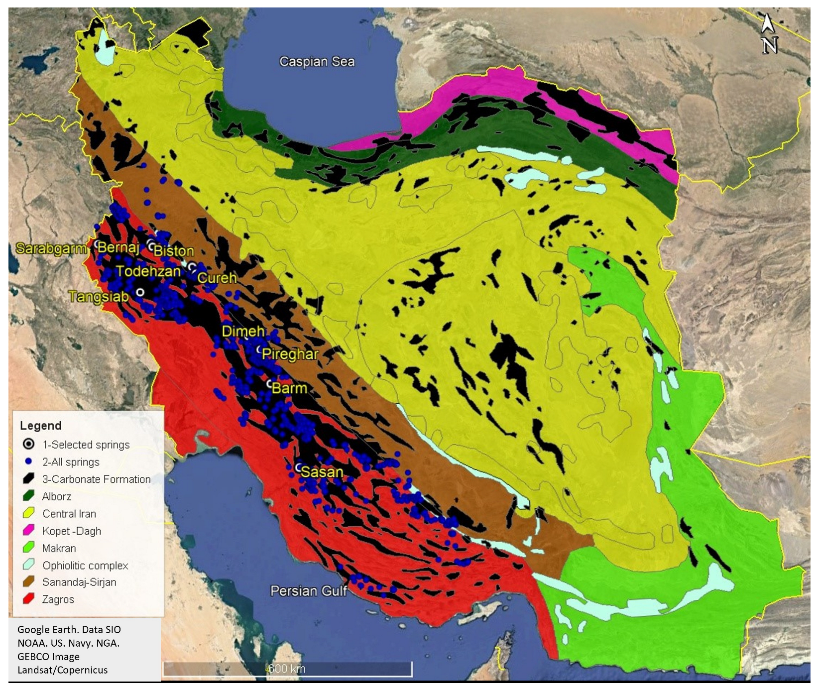
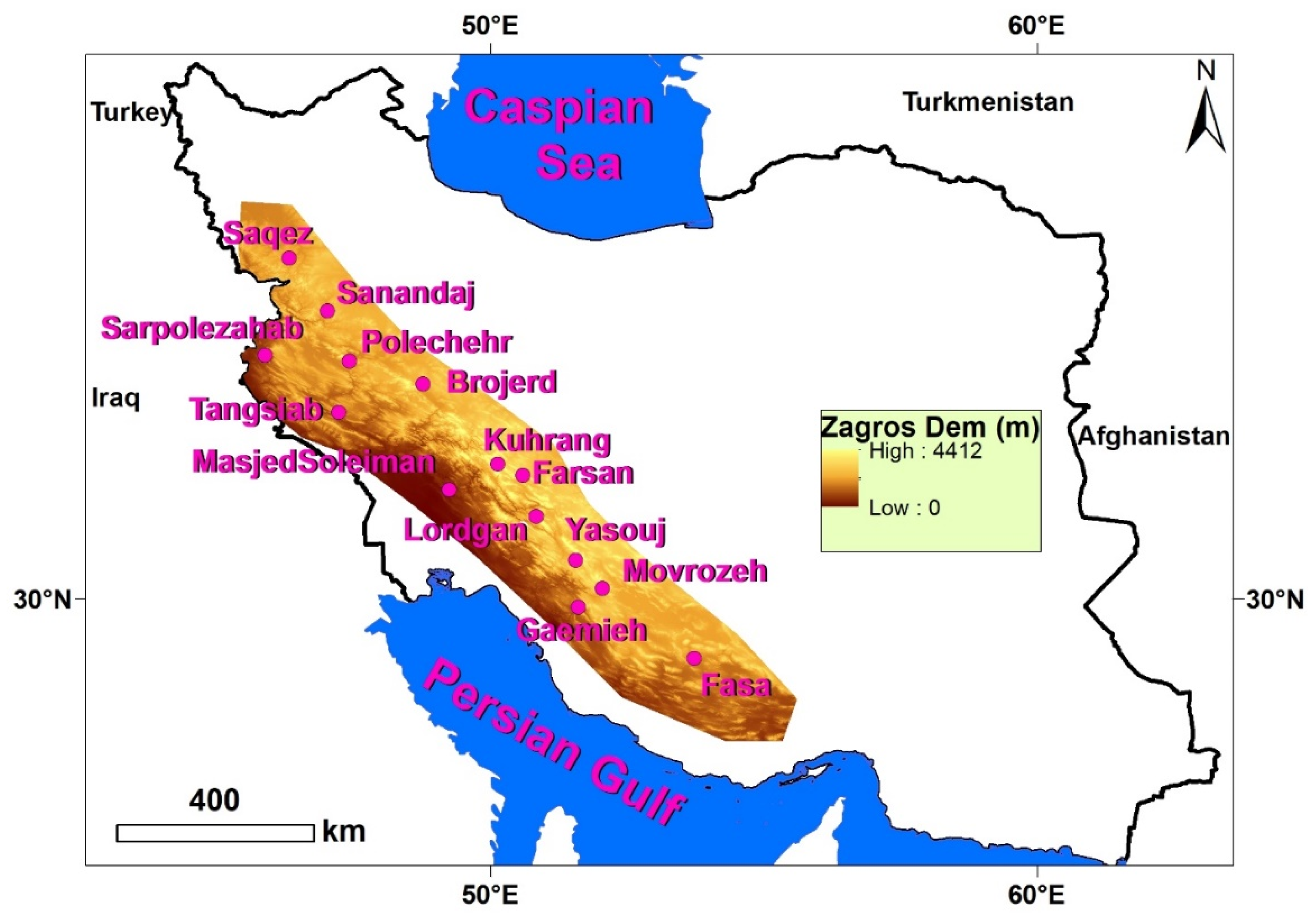
2. Study Area
3. Methodology
4. Results and Discussion
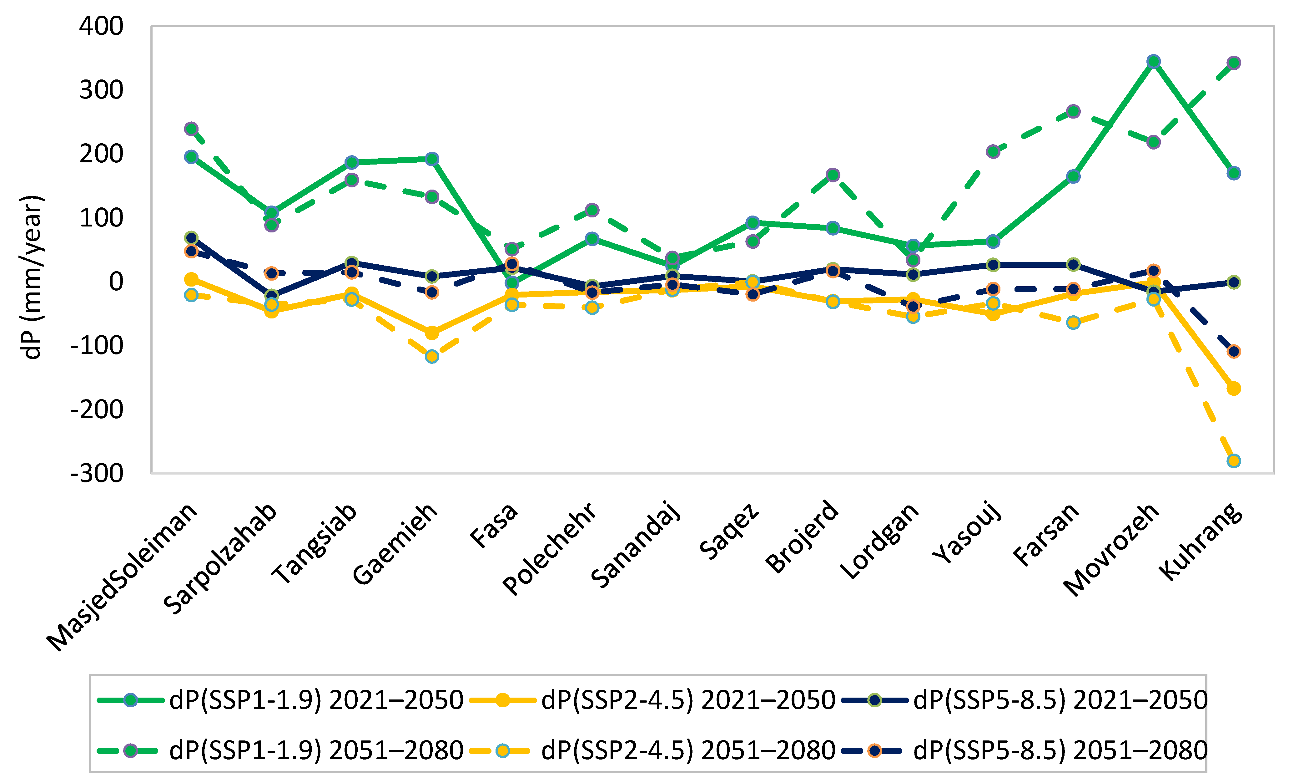
4.1. Precipitation under Climate Change
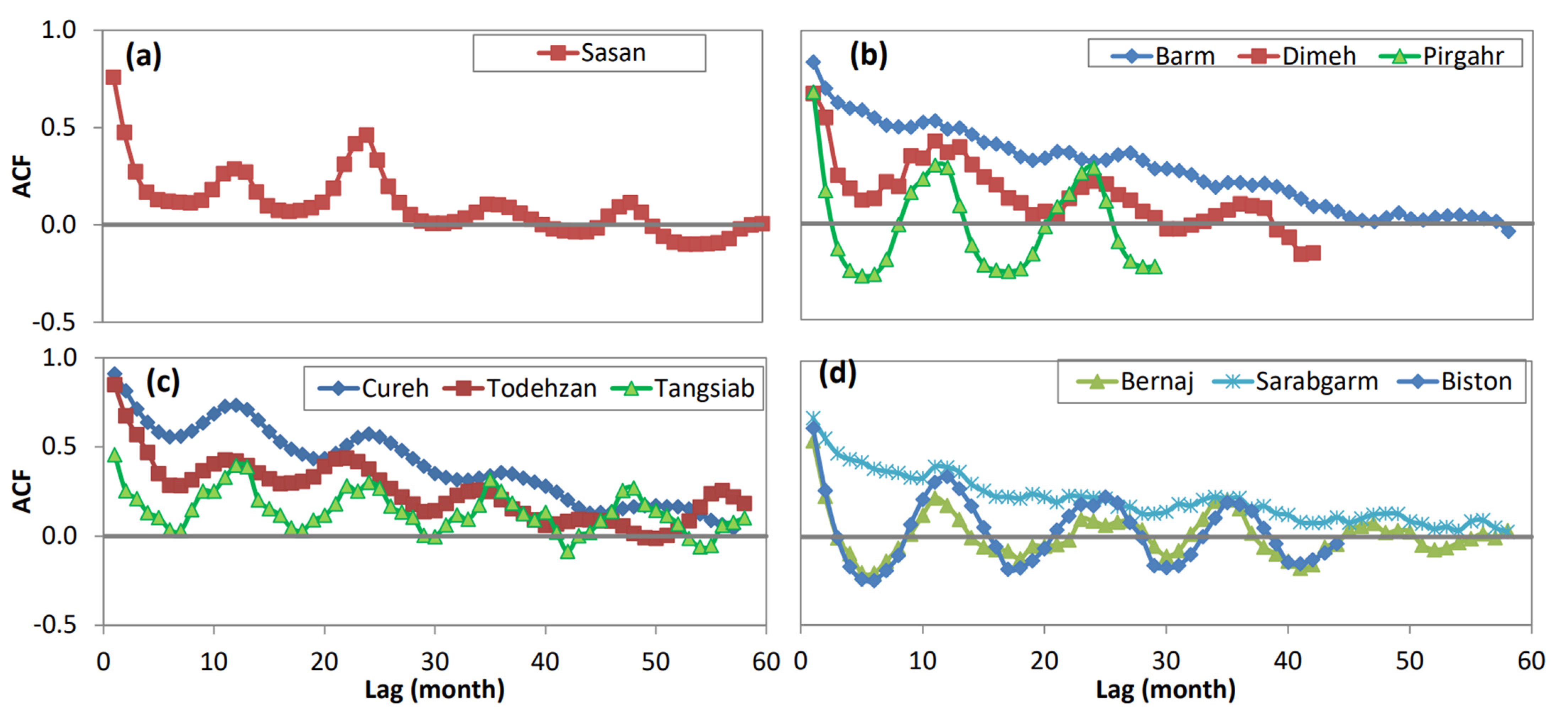
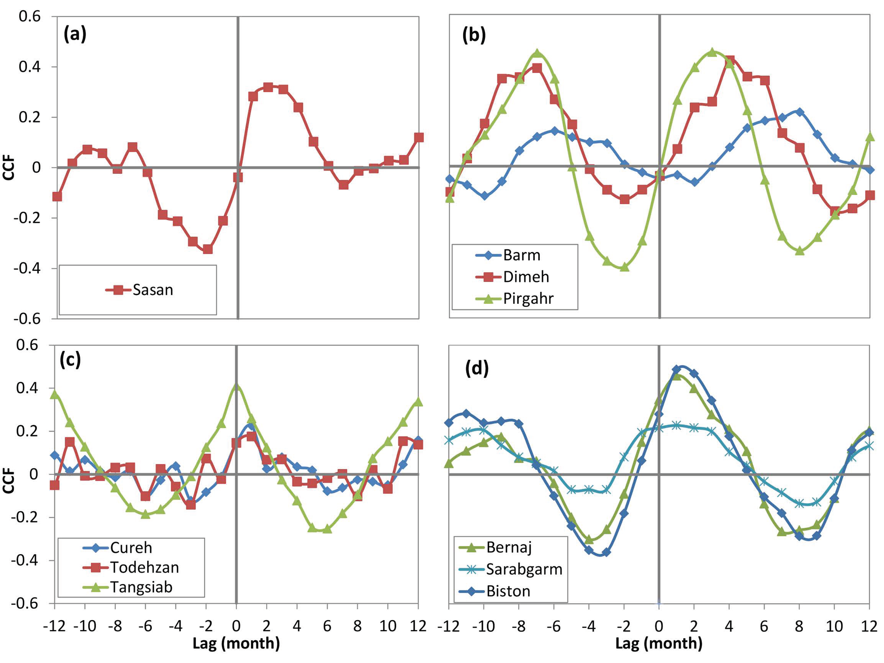
4.2. Time Series Analysis
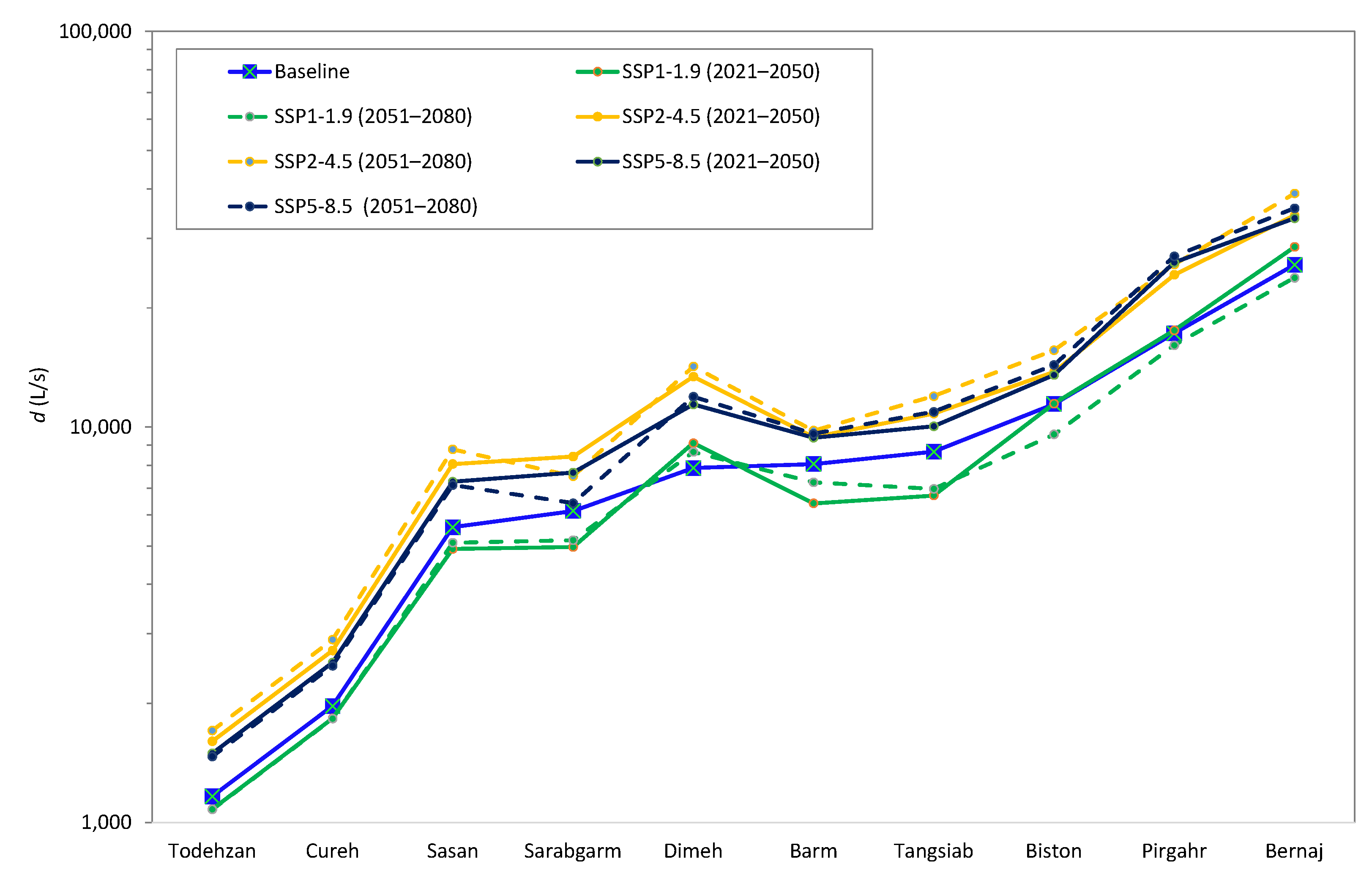
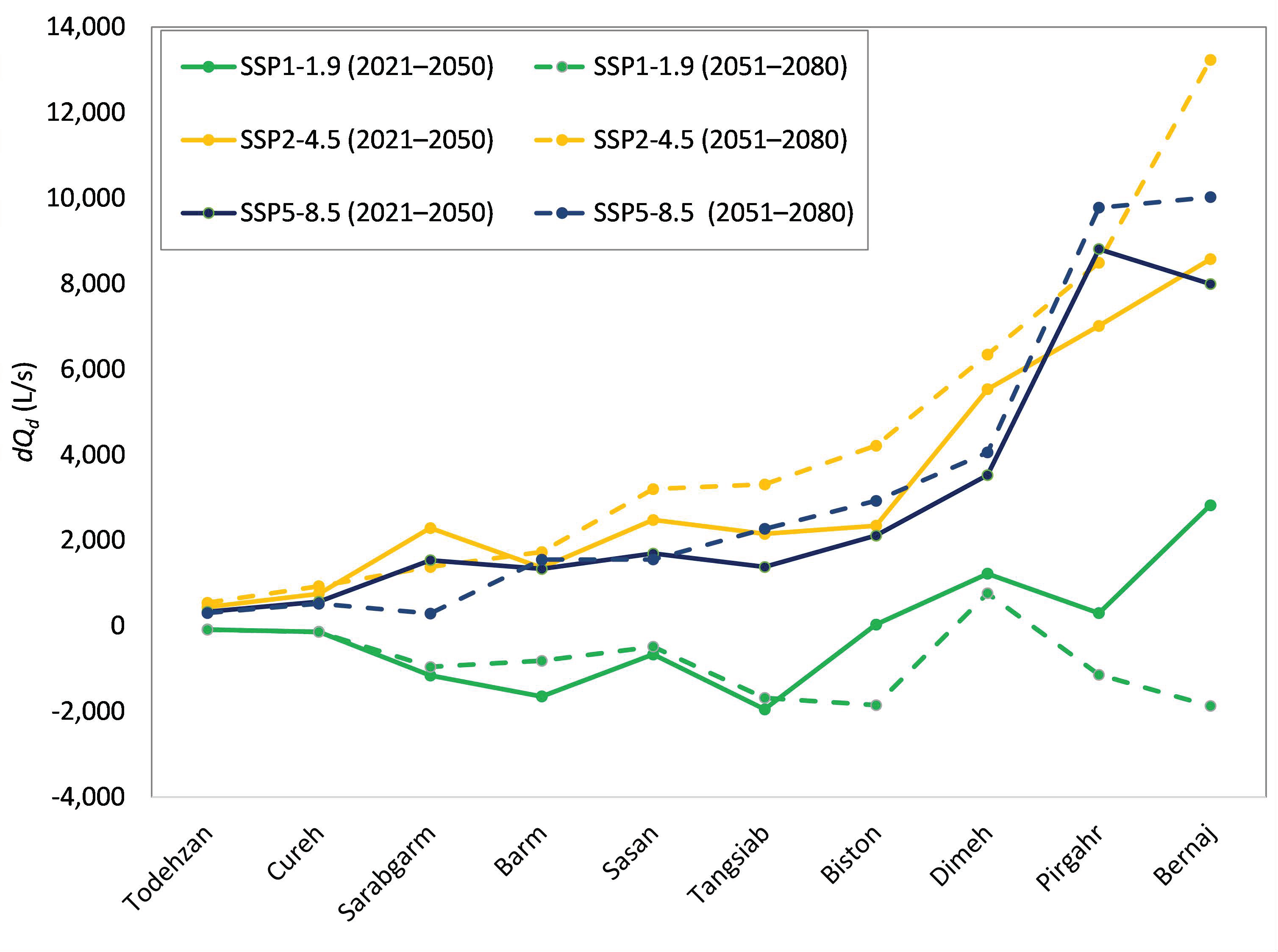
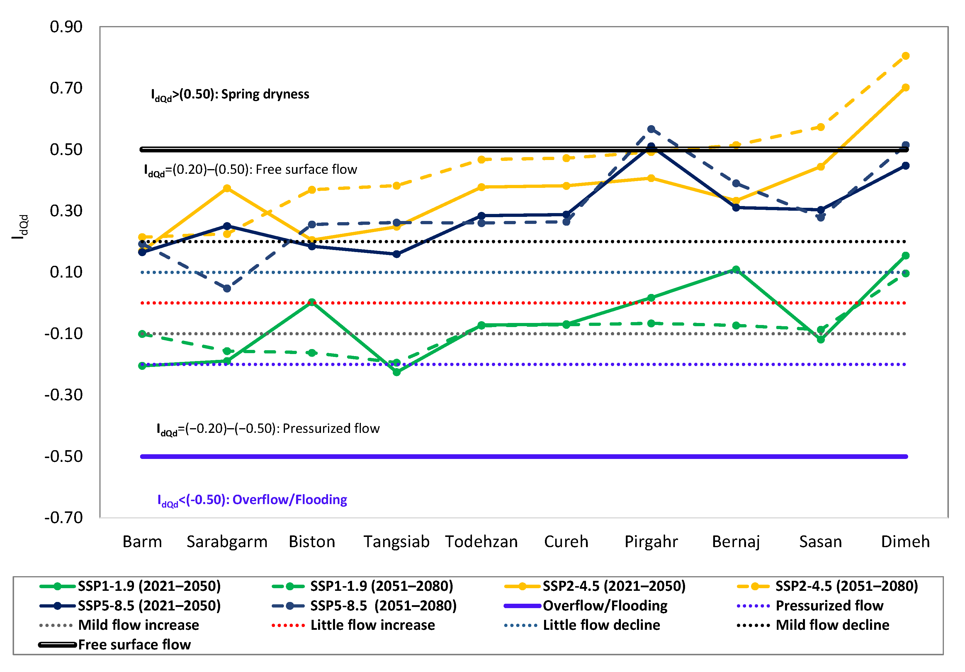
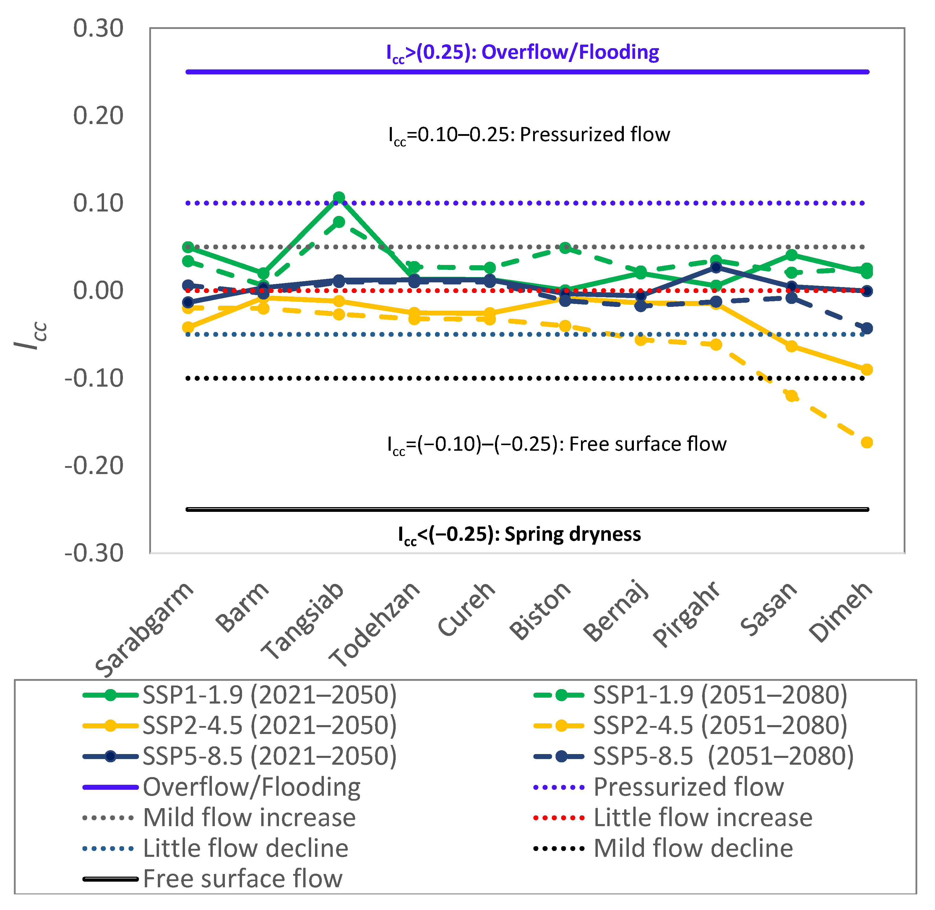
4.3. Flow Rate under Climate Change
4.4. Limitations and Uncertainties
5. Conclusions
Author Contributions
Funding
Institutional Review Board Statement
Informed Consent Statement
Data Availability Statement
Conflicts of Interest
Abbreviations
| ACF | autocorrelation analysis function |
| ANN | artificial neural network |
| CCF | cross correlation function |
| CGCM | coupled global climate model |
| CMIP6 | coupled model intercomparison project 6 |
| DEM | digital elevation model |
| GCM | general circulation models |
| GHGs | greenhouse gases |
| IPCC | intergovernmental panel on climate change |
| LARS-WG | Long Ashton Research Station weather generator |
| masl | meters above sea level |
| PCCF | partial cross correlation function |
| SDF | spectral density function |
| SSP | shared socio-economic pathway |
| SWAT | soil and water assessment tool |
| Notations | |
| the covariance function between rainfall and the springs flow rate | |
| Cxy (k) | the covariance function |
| d | square root of |
| dP | is the difference between the precipitation in the future climate change scenario (Pf) and the historical period (Pb) |
| variability of spring discharge from past to future | |
| variability index of spring discharge from past to future | |
| spring discharge variability over the historical data | |
| effect of precipitation and spring discharge change together | |
| the correlation coefficient between rainfall and the springs flow rate | |
| correlation between the elements of a series with other elements of the same series | |
| k | time lag |
| n | the length of a time series |
| N | the number of measurements |
| P | rainfall |
| Pb | precipitation in the historical period |
| Pf | precipitation in the future climate change scenario |
| Q | spring flow rate |
| Qmean | the average flow rate of the springs |
| Qt | the spring flow rate at any time |
| μx | the average of x |
| μy | the average of y |
| σx | the standard deviation of x |
| σy | the standard deviation of y |
| the standard deviation of the rainfall | |
| the standard deviation of the springs flow rate |
References
- Taylor, R.G.; Scanlon, B.; Döll, P.; Rodell, M.; Van Beek, R.; Wada, Y.; Longuevergne, L.; Leblanc, M.; Famiglietti, J.S.; Edmunds, M. Ground water and climate change. Nat. Clim. Chang. 2013, 3, 322–329. [Google Scholar] [CrossRef]
- Hartmann, A.; Jasechko, S.; Gleeson, T.; Wada, Y.; Andreo, B.; Barberá, J.A.; Brielmann, H.; Bouchaou, L.; Charlier, J.B.; Darling, W.G.; et al. Risk of groundwater contamination widely underestimated because of fast flow into aquifers. Proc. Natl. Acad. Sci. USA 2021, 118, e2024492118. [Google Scholar] [CrossRef] [PubMed]
- Stevanović, Z. Karst waters in potable water supply: A global scale overview. Environ. Earth Sci. 2019, 78, 662. [Google Scholar] [CrossRef]
- Quinlan, J.F.; Ewers, R.O. Subsurface drainage in the Mammoth Cave area. In Karst Hydrology; Springer: Boston, MA, USA, 1989; pp. 65–103. [Google Scholar]
- Hartmann, A.; Goldscheider, N.; Wagener, T.; Lange, J.; Weiler, M. Karst water resources in a changing world: Review of hydrological modeling approaches. Rev. Geophys. 2014, 52, 218–242. [Google Scholar] [CrossRef]
- Al-Charideh, A. Recharge rate estimation in the Mountain karst aquifer system of Figeh spring, Syria. Environ. Earth Sci. 2012, 65, 1169–1178. [Google Scholar] [CrossRef]
- Kresic, N.; Stevanovic, Z. (Eds.) Groundwater Hydrology of Springs: Engineering, Theory, Management and Sustainability; Butterworth-Heinemann: Waltham, MA, USA, 2009. [Google Scholar]
- Wu, P.; Tang, C.; Zhu, L.; Liu, C.; Cha, X.; Tao, X. Hydrogeochemical characteristics of surface water and groundwater in the karst basin, southwest China. Hydrol. Process. Int. J. 2009, 23, 2012–2022. [Google Scholar] [CrossRef]
- Gutiérrez, J.M.; San-Martín, D.; Brands, S.; Manzanas, R.; Herrera, S. Reassessing statistical downscaling techniques for their robust application under climate change conditions. J. Clim. 2013, 26, 171–188. [Google Scholar] [CrossRef]
- Semenov, M.A.; Barrow, E.M. A Stochastic Weather Generator for Use in Climate Impact Studies; User Man Herts: Hertfordshire, UK, 2002. [Google Scholar]
- Hassan, Z.; Shamsudin, S.; Harun, S. Application of SDSM and LARS-WG for simulating and downscaling of rainfall and temperature. Theor. Appl. Climatol. 2014, 116, 243–257. [Google Scholar] [CrossRef]
- IPCC. Summary for Policymakers. In Climate Change 2021: The Physical Science Basis. Contribution of Working Group I to the Sixth Assessment Report of the Intergovernmental Panel on Climate Change; Masson-Delmotte, V., Zhai, P., Pirani, A., Connors, S.L., Péan, C., Berger, S., Caud, N., Chen, Y., Goldfarb, L., Gomis, M.I., et al., Eds.; Cambridge University Press: Cambridge, UK, 2021. [Google Scholar]
- Eyring, V.; Bony, S.; Eyring Meehl, G.A.; Senior, C.A.; Stevens, B.; Stouffer, R.J.; Taylor, K.E. Overview of the Coupled Model Intercomparison Project Phase 6 (CMIP6) experimental design and organization. Geosci. Model Dev. 2016, 9, 1937–1958. [Google Scholar] [CrossRef]
- Dubois, E.; Doummar, J.; Pistre, S.; Larocque, M. Calibration of a lumped karst system model and application to the Qachqouch karst spring (Lebanon) under climate change conditions. Hydrol. Earth Syst. Sci. 2020, 24, 4275–4290. [Google Scholar] [CrossRef]
- Brouyère, S.; Carabin, G.; Dassargues, A. Climate change impacts on groundwater resources: Modelled deficits in a chalky aquifer, Geer basin, Belgium. Hydrogeol. J. 2004, 12, 123–134. [Google Scholar] [CrossRef]
- Pisinaras, V. Assessment of future climate change impacts in a Mediterranean aquifer. Glob. NEST J. 2016, 18, 119–130. [Google Scholar]
- Labat, D.; Ababou, R.; Mangin, A. Rainfall–runoff relations for karstic springs. Part II: Continuous wavelet and discrete orthogonal multiresolution analyses. J. Hydrol. 2000, 238, 149–178. [Google Scholar] [CrossRef]
- Charlier, J.B.; Ladouche, B.; Maréchal, J.C. Identifying the impact of climate and anthropic pressures on karst aquifers using wavelet analysis. J. Hydrol. 2004, 523, 610–623. [Google Scholar] [CrossRef]
- Pavlić, K.; Parlov, J. Cross-correlation and cross-spectral analysis of the hydrographs in the northern part of the Dinaric karst of Croatia. Geosciences 2019, 9, 86. [Google Scholar] [CrossRef]
- Denić-Jukić, V.; Lozić, A.; Jukić, D. An Application of Correlation and Spectral Analysis in Hydrological Study of Neighboring Karst Springs. Water 2020, 12, 3570. [Google Scholar] [CrossRef]
- Fiorillo, F.; Doglioni, A. The relation between karst spring discharge and rainfall by cross-correlation analysis (Campania, southern Italy). Hydrogeol. J. 2010, 18, 1881–1895. [Google Scholar] [CrossRef]
- Leone, G.; Pagnozzi, M.; Catani, V.; Ventafridda, G.; Esposito, L.; Fiorillo, F. A hundred years of Caposele spring discharge measurements: Trends and statistics for understanding water resource availability under climate change. Stoch. Environ. Res. Risk Assess. 2021, 35, 345–370. [Google Scholar] [CrossRef]
- Martín-Rodríguez, J.F.; Mudarra, M.; De la Torre, B.; Andreo, B. Towards a better understanding of time-lags in karst aquifers by combining hydrological analysis tools and dye tracer tests. Application to a binary karst aquifer in southern Spain. J. Hydrol. 2023, 621, 129643. [Google Scholar] [CrossRef]
- Abbaspour, K.C.; Faramarzi, M.; Ghasemi, S.S.; Yang, H. Assessing the impact of climate change on water resources in Iran. Water Resour. Res. 2009, 45. [Google Scholar] [CrossRef]
- Raeisi, E.; Kowsar, N. Development of Shahpour Cave, southern Iran. Cave Karst Sci. 1997, 24, 27–34. [Google Scholar]
- Vardanjani, H.K.; Bahadorinia, S.; Ford, D.C. An Introduction to Hypogene Karst Regions and Caves of Iran. In Hypogene Karst Regions and Caves of the World; Springer: Cham, Switzerland, 2017; pp. 479–494. [Google Scholar]
- Rostam Afshar, N.; Kazemi, H.; Nobahar, F. Quality Protection Legislations for Karst Water Resources. Iran-Water Resour. Res. 2010, 5, 56–58. [Google Scholar]
- Minoyi, M. The Role of Fractures in the Flow of Underground Water in the Karst Region of Shahu Mountains, Kurdistan. Master’s Thesis, Shahrood University of Technology, Shahrud, Iran, 2010. [Google Scholar]
- Zeydalinejad, N.; Nassery, H.R.; Alijani, F.; Shakiba, A. Forecasting the resilience of Bibitarkhoun karst spring, southwest Iran, to the future climate change. Model. Earth Syst. Environ. 2020, 6, 2359–2375. [Google Scholar] [CrossRef]
- Zeydalinejad, N.; Nassery, H.R.; Shakiba, A.; Alijani, F. Prediction of the karstic spring flow rates under climate change by climatic variables based on the artificial neural network: A case study of Iran. Environ. Monit. Assess. 2020, 192, 375. [Google Scholar] [CrossRef]
- Naderi, M.; Raeisi, E.; Zarei, M. The impact of halite dissolution of salt diapirs on surface and ground water under climate change, South-Central Iran. Environ. Earth Sci. 2016, 75, 708. [Google Scholar] [CrossRef]
- Peely, A.B.; Mohammadi, Z.; Raeisi, E. Breakthrough curves of dye tracing tests in karst aquifers: Review of effective parameters based on synthetic modeling and field data. J. Hydrol. 2021, 602, 126604. [Google Scholar] [CrossRef]
- Riedel, T.; Weber, T.K. The influence of global change on Europe’s water cycle and groundwater recharge. Hydrogeol. J. 2020, 28, 1939–1959. [Google Scholar] [CrossRef]
- Aghanabati, A. Geology of Iran; Organization of Geology and Mineral Explorations of Iran: Tehran, Iran, 2004. [Google Scholar]
- Moloudia, F.; Shokati, S. Assessment of Climate Change in Northern Zagros Forests using Stochastic Weather Generator; GeoConvention: Calgary, Canada, 2018. [Google Scholar]
- Hosseini, S.M.; Ataie-Ashtiani, B.; Simmons, C.T. Spring hydrograph simulation of karstic aquifers: Impacts of variable recharge area, intermediate storage and memory effects. J. Hydrol. 2017, 552, 225–240. [Google Scholar] [CrossRef]
- Dogančić, D.; Afrasiabian, A.; Kranjčić, N.; Đurin, B. Using Stable Isotope Analysis (δD and δ18O) and Tracing Tests to Characterize the Regional Hydrogeological Characteristics of Kazeroon County, Iran. Water 2020, 12, 2487. [Google Scholar] [CrossRef]
- Ford, D.; Williams, P.D. Karst Hydrogeology and Geomorphology; John Wiley & Sons: West Sussex, UK, 2007. [Google Scholar]
- Perne, M.; Covington, M.; Gabrovšek, F. Evolution of karst conduit networks in transition from pressurized flow to free-surface flow. Hydrol. Earth Syst. Sci. 2014, 18, 4617–4633. [Google Scholar] [CrossRef]
- Zoghbi, C.; Basha, H. Simplified physically based models for free-surface flow in karst systems. J. Hydrol. 2019, 578, 124040. [Google Scholar] [CrossRef]
- Mangin, A. Pour une meilleure connaissance des systèmes hydrologiques à partir des analyses corrélatoire et spectrale. J. Hydrol. 1984, 67, 25–43. [Google Scholar] [CrossRef]
- Raju, K.S.; Kumar, D.N. Review of approaches for selection and ensembling of GCMs. J. Water Clim. Chang. 2020, 11, 577–599. [Google Scholar] [CrossRef]
- Wang, H.M.; Chen, J.; Xu, C.Y.; Zhang, J.; Chen, H. A framework to quantify the uncertainty contribution of GCMs over multiple sources in hydrological impacts of climate change. Earths Future 2020, 8, e2020EF001602. [Google Scholar] [CrossRef]


| Spring | Mean Discharge Q (L/s) | Catchment Area (km2) | Q Trend | Meteorological Station | Elevation (m) | Rainfall P (mm/year) | P Trend |
|---|---|---|---|---|---|---|---|
| Todehzan | 158 | 171 | −0.01 | Brojerd | 1629 | 473 | 0.0003 |
| Cureh | 218 | 99.2 | −0.02 | Brojerd | 1629 | 473 | 0.0003 |
| Biston | 674 | 34.4 | −0.02 | Polechehr | 1270 | 372 | −0.00004 |
| Tangsiab | 1344 | 130 | −0.04 | Tangsiab | 900 | 394 | −0.0004 |
| Sasan | 1686 | 351 | −0.05 | Ghaemieh | 922 | 548 | −0.0007 |
| Pirgahr | 1818 | 72.1 | −0.12 | Farsan | 2062 | 414 | −0.0037 |
| Sarabgarm | 1824 | 62.9 | −0.06 | Sarpolezahab | 545 | 422 | −0.0011 |
| Bernaj | 1869 | 193 | −0.03 | Polechehr | 1270 | 372 | −0.00004 |
| Barm | 2183 | 556 | −0.05 | Lordgan | 1611 | 535 | −0.0009 |
| Dimeh | 2960 | 310 | −0.09 | Kuhrang | 2365 | 1309 | −0.0033 |
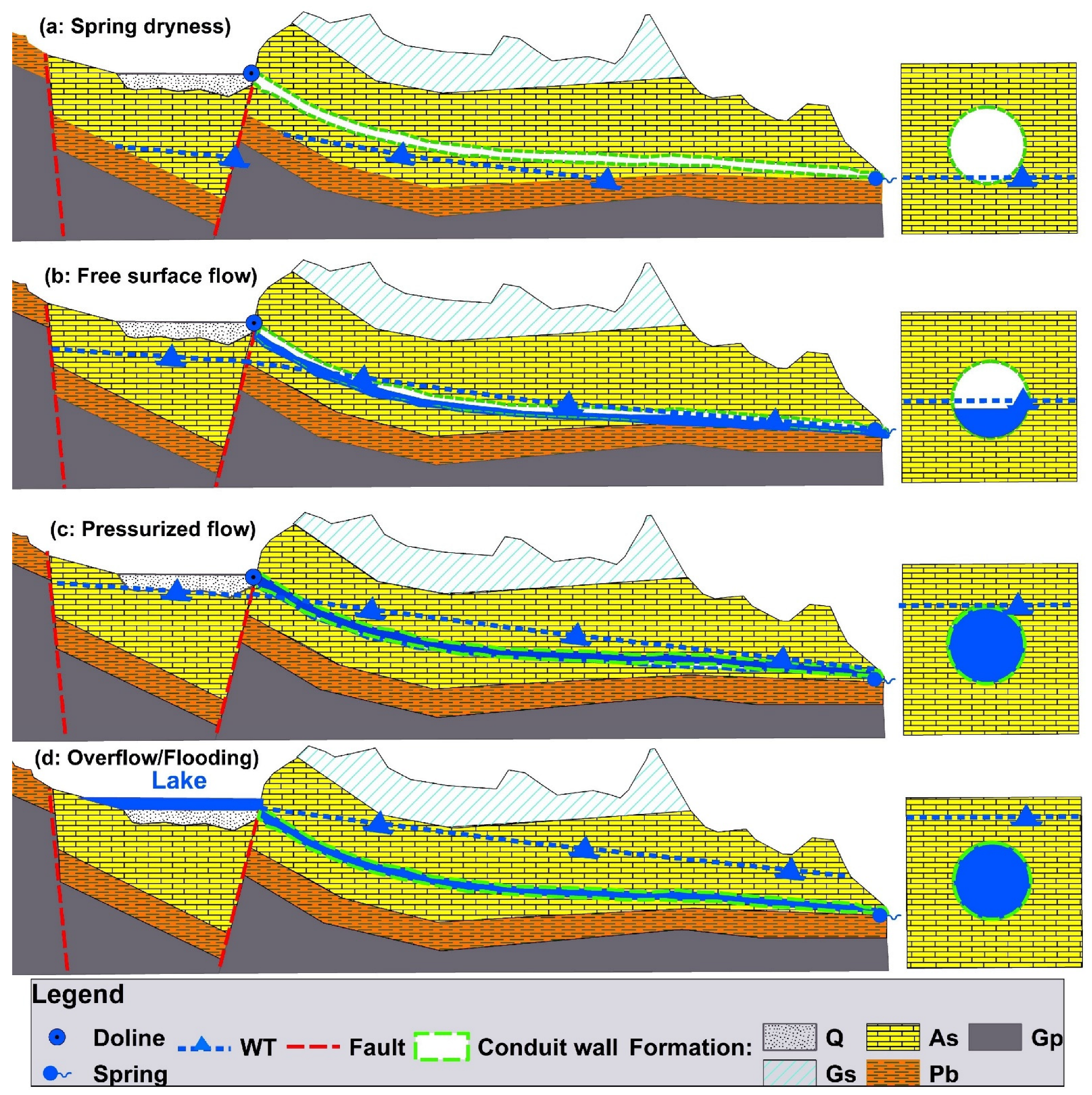
| Icc | Possible Corresponding Flow Conditions in Karst | Description | ||
|---|---|---|---|---|
| <0.50 | <(−0.50) | >0.25 | Overflow/Flooding | Groundwater flow is beyond conduit capacity; it recharges the matrix and the excess amount flows as runoff (back-flooding). |
| 0.50–0.80 | (−0.50)–(−0.20) | 0.10–0.25 | Pressurized flow | Groundwater flows in the whole cross section of conduits and it recharges the matrix. |
| 0.80–0.90 | (−0.20)–(−0.10) | 0.05–0.10 | Mild flow increase | The growth of groundwater flow is mild. |
| 0.90–1 | (−0.10)–0.00 | 0.00–0.05 | Little flow increase | There is no much difference with the previous flow conditions apart from a trivial flow rise. |
| 1–1.10 | 0.00–0.10 | (−0.05)–0.00 | Little flow decline | There is no much difference with the previous flow conditions apart from a trivial flow reduction. |
| 1.10–1.20 | 0.10–0.20 | (−0.05)–(−0.10) | Mild flow decline | The reduction in groundwater flow is mild |
| 1.20–1.50 | 0.20–0.50 | (−0.10)–(−0.25) | Free surface flow | Groundwater flows in some part of conduits and it discharges the matrix. |
| >1.50 | >0.50 | <(−0.25) | Spring dryness | The possibility of spring going dry is highly likely, especially in the event of low average rainfall and dominancy of conduit flow; soil-matrix flow may become dominant in case of soil layer existence. |
Disclaimer/Publisher’s Note: The statements, opinions and data contained in all publications are solely those of the individual author(s) and contributor(s) and not of MDPI and/or the editor(s). MDPI and/or the editor(s) disclaim responsibility for any injury to people or property resulting from any ideas, methods, instructions or products referred to in the content. |
© 2024 by the authors. Licensee MDPI, Basel, Switzerland. This article is an open access article distributed under the terms and conditions of the Creative Commons Attribution (CC BY) license (https://creativecommons.org/licenses/by/4.0/).
Share and Cite
Behrouj Peely, A.; Mohammadi, Z.; Sivelle, V.; Labat, D.; Naderi, M. A New Index to Assess the Effect of Climate Change on Karst Spring Flow Rate. Sustainability 2024, 16, 1326. https://doi.org/10.3390/su16031326
Behrouj Peely A, Mohammadi Z, Sivelle V, Labat D, Naderi M. A New Index to Assess the Effect of Climate Change on Karst Spring Flow Rate. Sustainability. 2024; 16(3):1326. https://doi.org/10.3390/su16031326
Chicago/Turabian StyleBehrouj Peely, Ahmad, Zargham Mohammadi, Vianney Sivelle, David Labat, and Mostafa Naderi. 2024. "A New Index to Assess the Effect of Climate Change on Karst Spring Flow Rate" Sustainability 16, no. 3: 1326. https://doi.org/10.3390/su16031326
APA StyleBehrouj Peely, A., Mohammadi, Z., Sivelle, V., Labat, D., & Naderi, M. (2024). A New Index to Assess the Effect of Climate Change on Karst Spring Flow Rate. Sustainability, 16(3), 1326. https://doi.org/10.3390/su16031326