
Comparing the Utility of Artificial Neural Networks (ANN) and Convolutional Neural Networks (CNN) on Sentinel-2 MSI to Estimate Dry Season Aboveground Grass Biomass

 ,
,  ,
,  ,
,  and
and
Abstract
1. Introduction
2. Methods
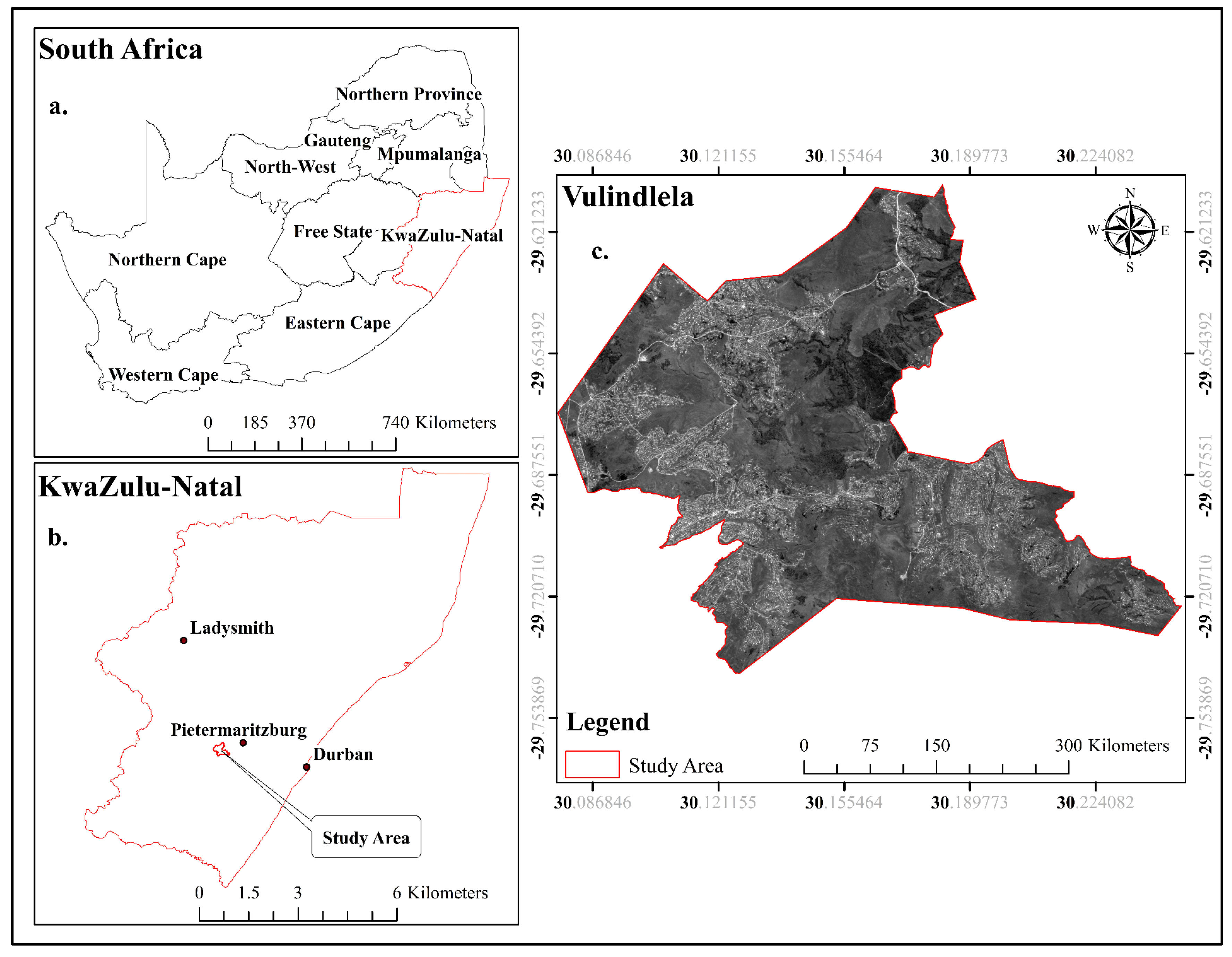
2.1. Study Area
2.2. Sentinel-2 MSI Satellite Imagery
2.3. Field Data Collection and Measurements
2.4. Vegetation Indices
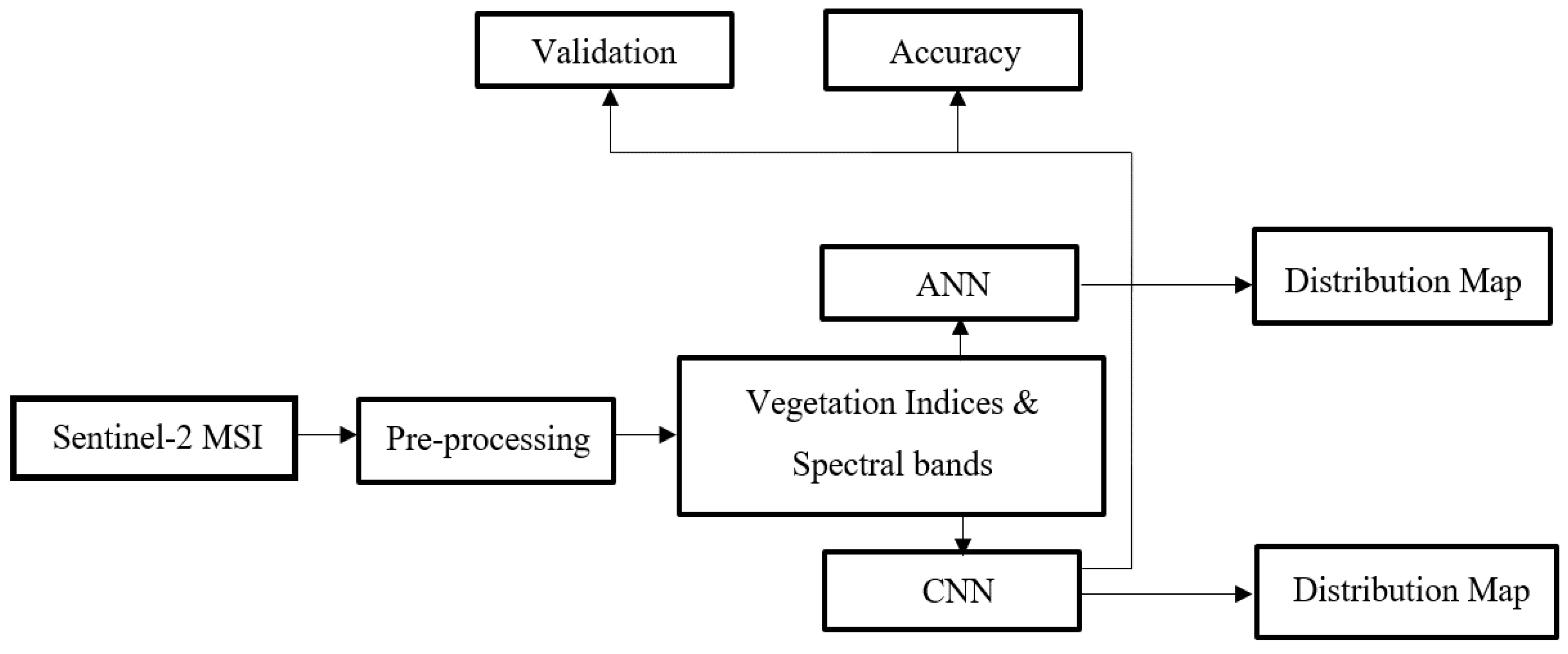
2.5. Statistical Analysis and Machine Learning
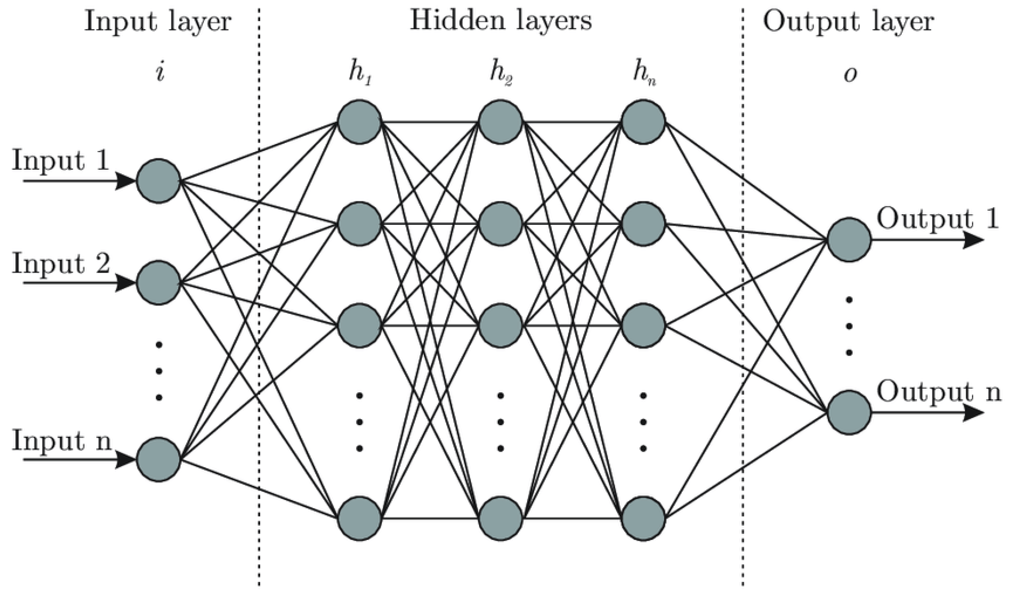
2.5.1. Artificial Neural Network (ANN)
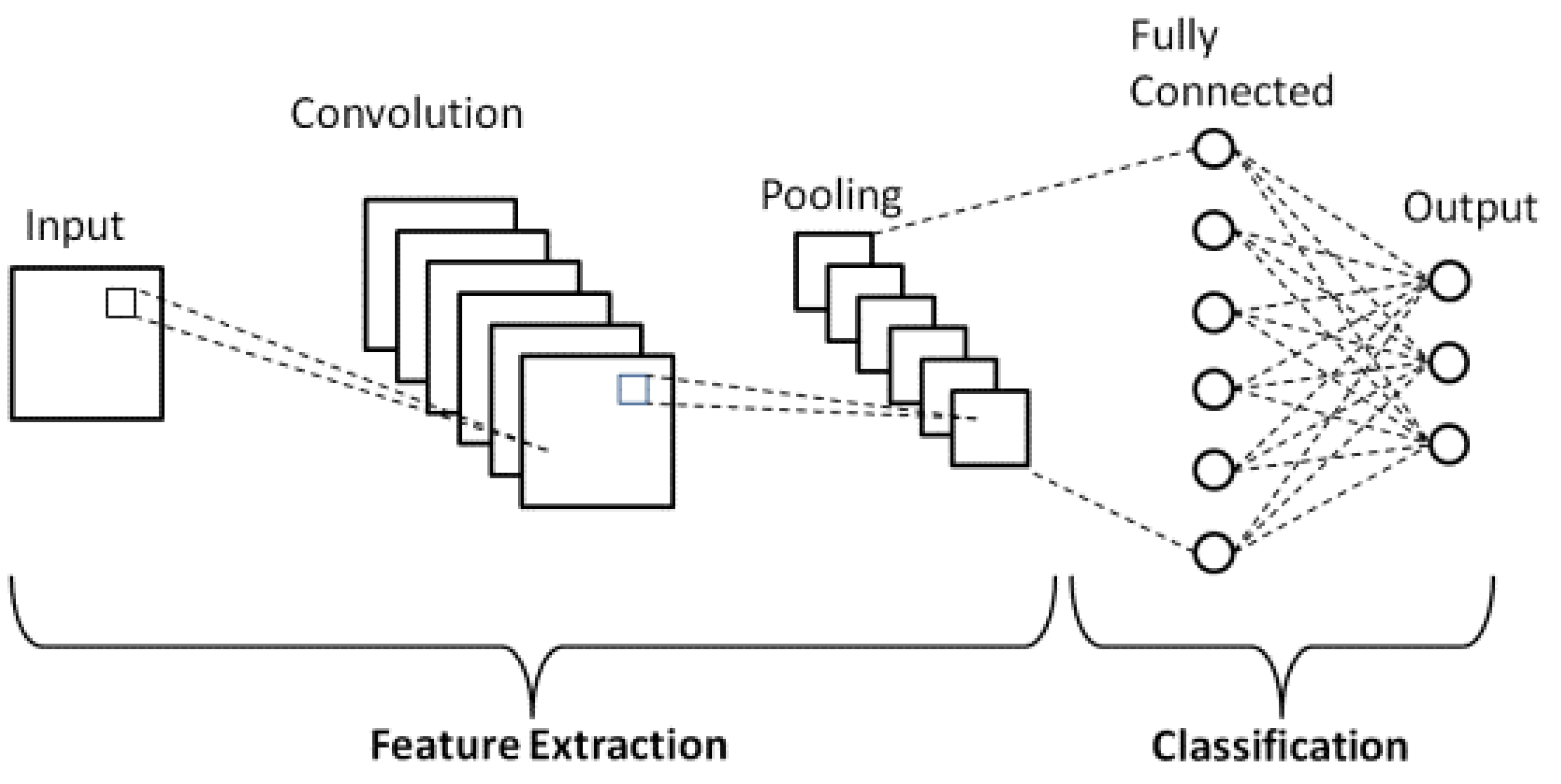
2.5.2. Convolutional Neural Network (CNN)
2.6. Accuracy Assessment
3. Results
3.1. Descriptive Statistics
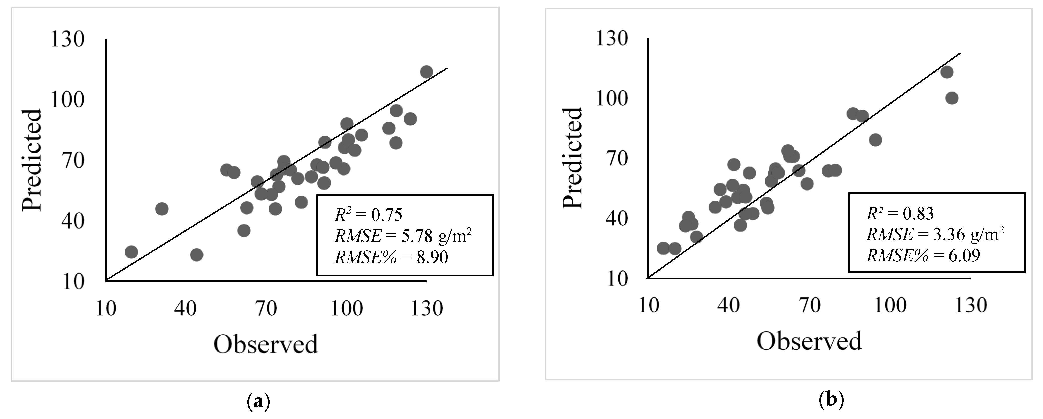
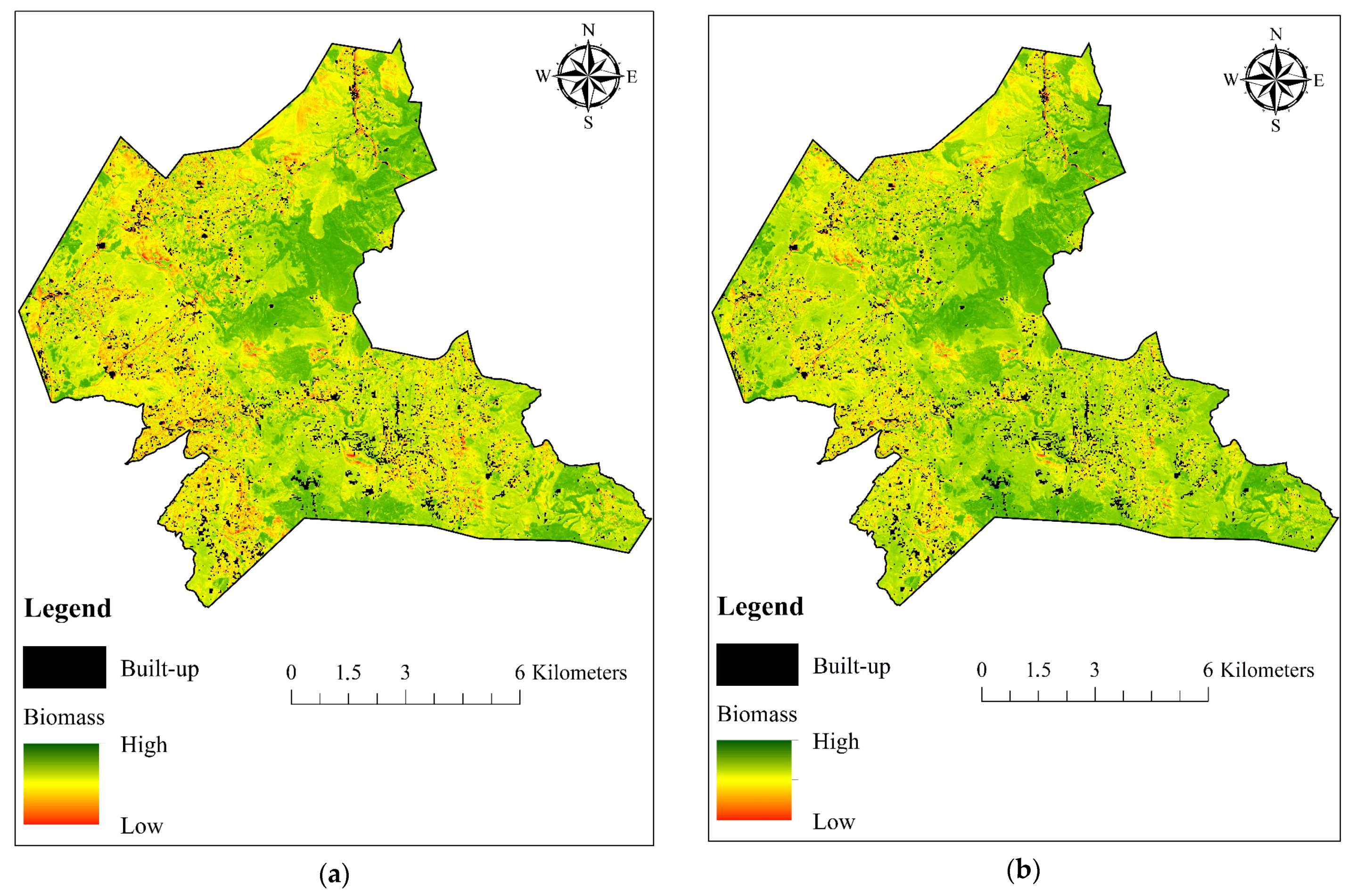
3.2. ANN vs. CNN
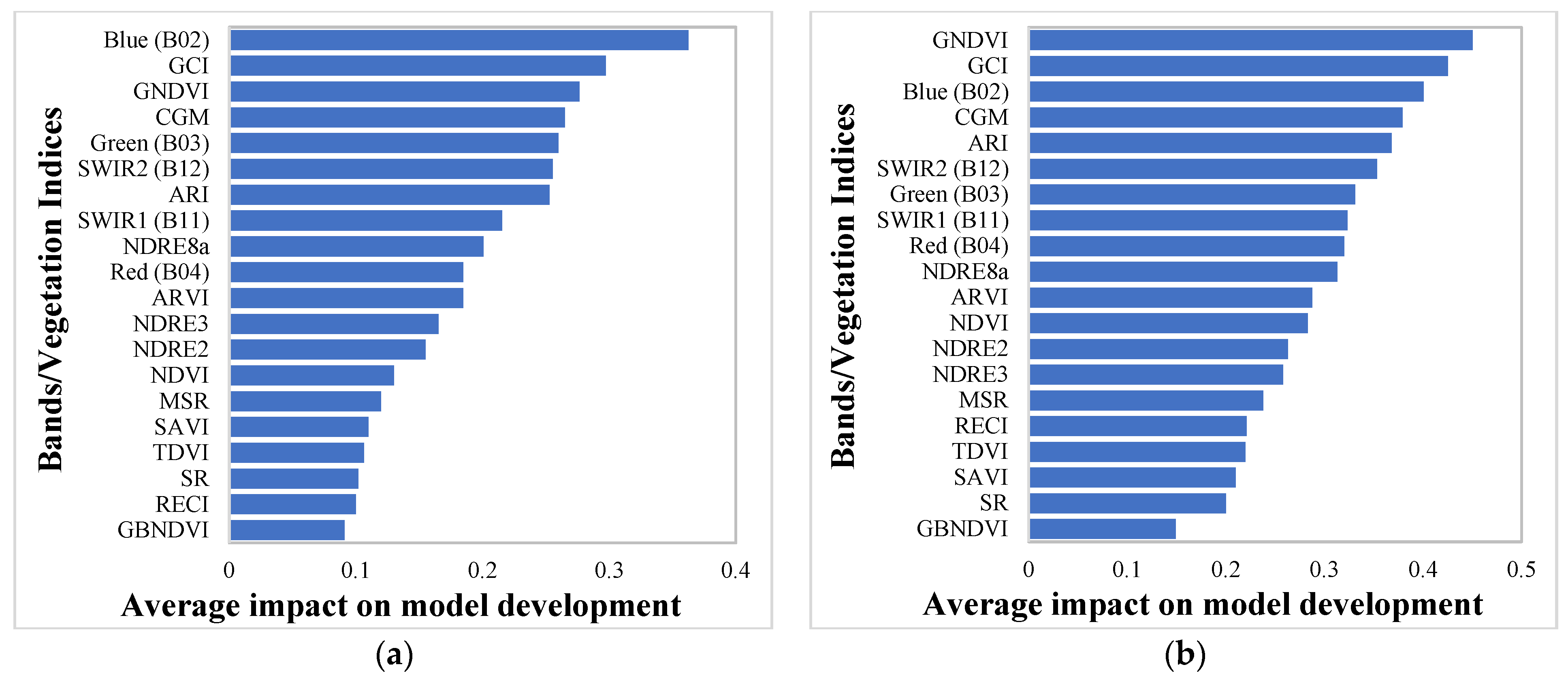
Sensitivity Analysis
4. Discussion
5. Conclusions
Author Contributions
Funding
Institutional Review Board Statement
Informed Consent Statement
Data Availability Statement
Acknowledgments
Conflicts of Interest
References
- Ali, I.; Greifeneder, F.; Stamenkovic, J.; Neumann, M.; Notarnicola, C. Review of Machine Learning Approaches for Biomass and Soil Moisture Retrievals from Remote Sensing Data. Remote Sens. 2015, 7, 16398–16421. [Google Scholar] [CrossRef]
- Mutanga, O.; Dube, T.; Ahmed, F. Progress in Remote Sensing: Vegetation Monitoring in South Africa. South Afr. Geogr. J. 2016, 98, 461–471. [Google Scholar] [CrossRef]
- Das, M.; Ghosh, S.K.; Chowdary, V.M.; Mitra, P.; Rijal, S. Statistical and Machine Learning Models for Remote Sensing Data Mining—Recent Advancements. Remote Sens. 2022, 14, 1906. [Google Scholar] [CrossRef]
- Mas, J.F.; Flores, J.J. The Application of Artificial Neural Networks to the Analysis of Remotely Sensed Data. Int. J. Remote Sens. 2008, 29, 617–663. [Google Scholar] [CrossRef]
- Jensen, R.R.; Hardin, P.J.; Yu, G. Artificial Neural Networks and Remote Sensing. Geogr. Compass 2009, 3, 630–646. [Google Scholar] [CrossRef]
- Liu, X.; Han, F.; Ghazali, K.H.; Mohamed, I.I.; Zhao, Y. A Review of Convolutional Neural Networks in Remote Sensing Image. In Proceedings of the 2019 8th International Conference on Software and Computer Applications, Penang, Malaysia, 19–21 February 2019; pp. 263–267. [Google Scholar]
- Zhu, X.X.; Tuia, D.; Mou, L.; Xia, G.-S.; Zhang, L.; Xu, F.; Fraundorfer, F. Deep Learning in Remote Sensing: A Comprehensive Review and List of Resources. IEEE Geosci. Remote Sens. Mag. 2017, 5, 8–36. [Google Scholar] [CrossRef]
- Kattenborn, T.; Leitloff, J.; Schiefer, F.; Hinz, S. Review on Convolutional Neural Networks (CNN) in Vegetation Remote Sensing. ISPRS J. Photogramm. Remote Sens. 2021, 173, 24–49. [Google Scholar] [CrossRef]
- Brodrick, P.G.; Davies, A.B.; Asner, G.P. Uncovering Ecological Patterns with Convolutional Neural Networks. Trends Ecol. Evol. 2019, 34, 734–745. [Google Scholar] [CrossRef]
- Palmer, A.; Short, A.; Yunusa, I.A. Biomass Production and Water Use Efficiency of Grassland in KwaZulu-Natal, South Africa. Afr. J. Range Forage Sci. 2010, 27, 163–169. [Google Scholar] [CrossRef]
- Vundla, T.; Mutanga, O.; Sibanda, M. Quantifying Grass Productivity Using Remotely Sensed Data: An Assessment of Grassland Restoration Benefits. Afr. J. Range Forage Sci. 2020, 37, 247–256. [Google Scholar] [CrossRef]
- Clementini, C.; Pomente, A.; Latini, D.; Kanamaru, H.; Vuolo, M.R.; Heureux, A.; Fujisawa, M.; Schiavon, G.; Del Frate, F. Long-term Grass Biomass Estimation of Pastures from Satellite Data. Remote Sens. 2020, 12, 2160. [Google Scholar] [CrossRef]
- Hoffman, T.; Vogel, C. Climate Change Impacts on African Rangelands. Rangelands 2008, 30, 12–17. [Google Scholar] [CrossRef]
- Soussana, J.-F.; Tallec, T.; Blanfort, V. Mitigating the Greenhouse Gas Balance of Ruminant Production Systems through Carbon Sequestration in Grasslands. Animal 2010, 4, 334–350. [Google Scholar] [CrossRef]
- Wei, J.; Cheng, J.; Li, W.; Liu, W. Comparing the Effect of Naturally Restored Forest and Grassland on Carbon Sequestration and Its Vertical Distribution in the Chinese Loess Plateau. PLoS ONE 2012, 7, e40123. [Google Scholar] [CrossRef]
- Masenyama, A.; Mutanga, O.; Dube, T.; Bangira, T.; Sibanda, M.; Mabhaudhi, T. A Systematic Review on the Use of Remote Sensing Technologies in Quantifying Grasslands Ecosystem Services. GIScience Remote Sens. 2022, 59, 1000–1025. [Google Scholar] [CrossRef]
- Sibanda, M.; Onisimo, M.; Dube, T.; Mabhaudhi, T. Quantitative Assessment of Grassland Foliar Moisture Parameters as an Inference on Rangeland Condition in the Mesic Rangelands of Southern Africa. Int. J. Remote Sens. 2021, 42, 1474–1491. [Google Scholar] [CrossRef]
- Fynn, R.; Morris, C.; Ward, D.; Kirkman, K. Trait–Environment Relations for Dominant Grasses in South African Mesic Grassland Support a General Leaf Economic Model. J. Veg. Sci. 2011, 22, 528–540. [Google Scholar] [CrossRef]
- Scott-Shaw, R.; Morris, C.D. Grazing Depletes Forb Species Diversity in the Mesic Grasslands of KwaZulu-Natal, South Africa. Afr. J. Range Forage Sci. 2015, 32, 21–31. [Google Scholar] [CrossRef]
- Masemola, C.; Cho, M.A.; Ramoelo, A. Sentinel-2 Time Series Based Optimal Features and Time Window for Mapping Invasive Australian Native Acacia Species in KwaZulu Natal, South Africa. Int. J. Appl. Earth Obs. Geoinf. 2020, 93, 102207. [Google Scholar] [CrossRef]
- Roffe, S.J.; Fitchett, J.M.; Curtis, C.J. Determining the Utility of a Percentile-Based Wet-Season Start-And End-Date Metrics across South Africa. Theor. Appl. Climatol. 2020, 140, 1331–1347. [Google Scholar] [CrossRef]
- EOS Data Analytics. Landviewer. Available online: https://eos.com/products/landviewer/ (accessed on 21 October 2021).
- Main-Knorn, M.; Pflug, B.; Louis, J.; Debaecker, V.; Müller-Wilm, U.; Gascon, F. Sen2Cor for Sentinel-2. In Proceedings of the Image and Signal Processing for Remote Sensing XXIII, Warsaw, Poland, 11–13 September 2017; p. 1042704. [Google Scholar]
- Shoko, C.; Mutanga, O.; Dube, T.; Slotow, R. Characterizing the Spatio-Temporal Variations of C3 and C4 Dominated Grasslands Aboveground Biomass in the Drakensberg, South Africa. Int. J. Appl. Earth Obs. Geoinf. 2018, 68, 51–60. [Google Scholar] [CrossRef]
- EOS Data Analytics. Sentinel 2 Satellite Images. Available online: https://eos.com/find-satellite/sentinel-2/ (accessed on 21 October 2021).
- Royimani, L.; Mutanga, O.; Odindi, J.; Sibanda, M.; Chamane, S. Determining the Onset of Autumn Grass Senescence in Subtropical Sour-Veld Grasslands Using Remote Sensing Proxies and the Breakpoint Approach. Ecol. Inform. 2022, 69, 101651. [Google Scholar] [CrossRef]
- Ma, J.; Li, Y.; Chen, Y.; Du, K.; Zheng, F.; Zhang, L.; Sun, Z. Estimating above Ground Biomass of Winter Wheat at Early Growth Stages Using Digital Images and Deep Convolutional Neural Network. Eur. J. Agron. 2019, 103, 117–129. [Google Scholar] [CrossRef]
- ESRI. Available online: www.esri.com (accessed on 18 October 2021).
- Huete, A.; Didan, K.; Miura, T.; Rodriguez, E.P.; Gao, X.; Ferreira, L.G. Overview of the Radiometric and Biophysical Performance of the MODIS Vegetation Indices. Remote Sens. Environ. 2002, 83, 195–213. [Google Scholar] [CrossRef]
- Huete, A.R. A Soil-Adjusted Vegetation Index (SAVI). Remote Sens. Environ. 1988, 25, 295–309. [Google Scholar] [CrossRef]
- Roujean, J.-L.; Breon, F.-M. Estimating PAR Absorbed by Vegetation from Bidirectional Reflectance Measurements. Remote Sens. Environ. 1995, 51, 375–384. [Google Scholar] [CrossRef]
- Chen, J.M. Evaluation of Vegetation Indices and a Modified Simple Ratio for Boreal Applications. Can. J. Remote Sens. 1996, 22, 229–242. [Google Scholar] [CrossRef]
- Fernández-Manso, A.; Fernández-Manso, O.; Quintano, C. Sentinel-2a Red-Edge Spectral Indices Suitability for Discriminating Burn Severity. Int. J. Appl. Earth Obs. Geoinf. 2016, 50, 170–175. [Google Scholar] [CrossRef]
- Santoso, H.; Gunawan, T.; Jatmiko, R.H.; Darmosarkoro, W.; Minasny, B. Mapping and Identifying Basal Stem Rot Disease in Oil Palms in North Sumatra with Quickbird Imagery. Precis. Agric. 2011, 12, 233–248. [Google Scholar] [CrossRef]
- Gitelson, A.A.; Merzlyak, M.N. Remote Estimation of Chlorophyll Content in Higher Plant Leaves. Int. J. Remote Sens. 1997, 18, 2691–2697. [Google Scholar] [CrossRef]
- Gamon, J.; Surfus, J. Assessing Leaf Pigment Content and Activity with a Reflectometer. New Phytol. 1999, 143, 105–117. [Google Scholar] [CrossRef]
- Kaufman, Y.J.; Tanre, D. Strategy for Direct and Indirect Methods for Correcting the Aerosol Effect on Remote Sensing: From Avhrr to Eos-Modis. Remote Sens. Environ. 1996, 55, 65–79. [Google Scholar] [CrossRef]
- Bannari, A.; Asalhi, H.; Teillet, P.M. Transformed Difference Vegetation Index (TDVI) for Vegetation Cover Mapping. In Proceedings of the IEEE International Geoscience and Remote Sensing Symposium, Toronto, ON, Canada, 24–28 June 2002; pp. 3053–3055. [Google Scholar]
- Tucker, C.J. Red and Photographic Infrared Linear Combinations for Monitoring Vegetation. Remote Sens. Environ. 1979, 8, 127–150. [Google Scholar] [CrossRef]
- Guerini Filho, M.; Kuplich, T.M.; Quadros, F.L.D. Estimating Natural Grassland Biomass by Vegetation Indices Using Sentinel 2 Remote Sensing Data. Int. J. Remote Sens. 2020, 41, 2861–2876. [Google Scholar] [CrossRef]
- Kobayashi, N.; Tani, H.; Wang, X.; Sonobe, R. Crop Classification Using Spectral Indices Derived from Sentinel-2a Imagery. J. Inf. Telecommun. 2020, 4, 67–90. [Google Scholar] [CrossRef]
- Clevers, J.G.; Gitelson, A.A. Remote Estimation of Crop and Grass Chlorophyll and Nitrogen Content Using Red-Edge Bands on Sentinel-2 and-3. Int. J. Appl. Earth Obs. Geoinf. 2013, 23, 344–351. [Google Scholar] [CrossRef]
- Yang, S.; Feng, Q.; Liang, T.; Liu, B.; Zhang, W.; Xie, H. Modeling Grassland Above-Ground Biomass Based on Artificial Neural Network and Remote Sensing in the Three-River Headwaters Region. Remote Sens. Environ. 2018, 204, 448–455. [Google Scholar] [CrossRef]
- Deb, D.; Singh, J.; Deb, S.; Datta, D.; Ghosh, A.; Chaurasia, R. An Alternative Approach for Estimating above Ground Biomass Using Resourcesat-2 Satellite Data and Artificial Neural Network in Bundelkhand Region of India. Environ. Monit. Assess. 2017, 189, 576. [Google Scholar] [CrossRef]
- Pires de Lima, R.; Marfurt, K. Convolutional Neural Network for Remote-Sensing Scene Classification: Transfer Learning Analysis. Remote Sens. 2020, 12, 86. [Google Scholar] [CrossRef]
- Schreiber, L.V.; Atkinson Amorim, J.G.; Guimarães, L.; Motta Matos, D.; Maciel da Costa, C.; Parraga, A. Above-ground Biomass Wheat Estimation: Deep Learning with UAV-based RGB Images. Appl. Artif. Intell. 2022, 36, 2055392. [Google Scholar] [CrossRef]
- Li, C.; Zhou, L.; Xu, W. Estimating Aboveground Biomass Using Sentinel-2 MSI Data and Ensemble Algorithms for Grassland in the Shengjin Lake Wetland, China. Remote Sens. 2021, 13, 1595. [Google Scholar] [CrossRef]
- Ali, I.; Cawkwell, F.; Dwyer, E.; Green, S. Modeling Managed Grassland Biomass Estimation by Using Multitemporal Remote Sensing Data—A Machine Learning Approach. IEEE J. Sel. Top. Appl. Earth Obs. Remote Sens. 2016, 10, 3254–3264. [Google Scholar] [CrossRef]
- Dong, L.; Du, H.; Han, N.; Li, X.; Zhu, D.e.; Mao, F.; Zhang, M.; Zheng, J.; Liu, H.; Huang, Z. Application of Convolutional Neural Network on Lei Bamboo above-Ground-Biomass (AGB) Estimation Using Worldview-2. Remote Sens. 2020, 12, 958. [Google Scholar] [CrossRef]
- Xie, Y.; Sha, Z.; Yu, M.; Bai, Y.; Zhang, L. A Comparison of Two Models with Landsat Data for Estimating above ground Grassland Biomass in Inner Mongolia, China. Ecol. Model. 2009, 220, 1810–1818. [Google Scholar] [CrossRef]
- Karila, K.; Alves Oliveira, R.; Ek, J.; Kaivosoja, J.; Koivumäki, N.; Korhonen, P.; Niemeläinen, O.; Nyholm, L.; Näsi, R.; Pölönen, I. Estimating Grass Sward Quality and Quantity Parameters Using Drone Remote Sensing with Deep Neural Networks. Remote Sens. 2022, 14, 2692. [Google Scholar] [CrossRef]
- Varela, S.; Zheng, X.-Y.; Njuguna, J.; Sacks, E.; Allen, D.; Ruhter, J.; Leakey, A.D. Deep Convolutional Neural Networks Exploit High Spatial and Temporal Resolution Aerial Imagery to Predict Key Traits in Miscanthus. AgriRxiv 2022, 20220405560. [Google Scholar] [CrossRef]
- Ramoelo, A.; Cho, M.A. Dry Season Biomass Estimation as an Indicator of Rangeland Quantity Using Multi-Scale Remote Sensing Data. 2014. Available online: http://pta-dspace-dmz.csir.co.za/dspace/handle/10204/7852 (accessed on 26 October 2021).
- Pang, H.; Zhang, A.; Kang, X.; He, N.; Dong, G. Estimation of the Grassland Aboveground Biomass of the Inner Mongolia Plateau Using the Simulated Spectra of Sentinel-2 Images. Remote Sens. 2020, 12, 4155. [Google Scholar] [CrossRef]
- Dusseux, P.; Guyet, T.; Pattier, P.; Barbier, V.; Nicolas, H. Monitoring of Grassland Productivity Using Sentinel-2 Remote Sensing Data. Int. J. Appl. Earth Obs. Geoinf. 2022, 111, 102843. [Google Scholar] [CrossRef]
- Muro, J.; Linstädter, A.; Magdon, P.; Wöllauer, S.; Männer, F.A.; Schwarz, L.-M.; Ghazaryan, G.; Schultz, J.; Malenovský, Z.; Dubovyk, O. Predicting Plant Biomass and Species Richness in Temperate Grasslands across Regions, Time, and Land Management with Remote Sensing and Deep Learning. Remote Sens. Environ. 2022, 282, 113262. [Google Scholar] [CrossRef]
- Ali, I.; Cawkwell, F.; Dwyer, E.; Barrett, B.; Green, S. Satellite Remote Sensing of Grasslands: From Observation to Management. J. Plant Ecol. 2016, 9, 649–671. [Google Scholar] [CrossRef]


| Band Number | Band Name | Central Wavelength (nm) | Bandwidth (nm) | Resolution (m) |
|---|---|---|---|---|
| 1 | Coastal aerosol | 442.3 | 20 | 60 |
| 2 | Blue | 492.1 | 65 | 10 |
| 3 | Green | 559 | 35 | 10 |
| 4 | Red | 665 | 30 | 10 |
| 5 | Red edge 1 | 703.8 | 15 | 20 |
| 6 | Red edge 2 | 739.1 | 15 | 20 |
| 7 | Red edge 3 | 779.7 | 20 | 20 |
| 8 | NIR | 833 | 115 | 10 |
| 8a | Red edge 8a | 864 | 20 | 20 |
| 9 | Water vapour | 943.2 | 20 | 60 |
| 10 | SWIR-Cirrus | 1376.9 | 30 | 60 |
| 11 | SWIR 1 | 1610.4 | 90 | 20 |
| 12 | SWIR 2 | 2185.7 | 180 | 20 |
| Vegetation Index | Abbreviation | Formula | Reference |
|---|---|---|---|
| Broadband VIs | |||
| Enhanced Vegetation Index | EVI | [29] | |
| Soil adjusted vegetation index | SAVI | [30] | |
| Normalised difference vegetation index | NDVI | [30] | |
| Renormalised difference vegetation index | RDVI | [31] | |
| Simple ratio | SR | [32] | |
| Modified simple ratio | MSR | [32] | |
| Green normalised difference vegetation index | GNDVI | [33] | |
| Green-blue normalised difference vegetation index | GBNDVI | [34] | |
| Chlorophyll green index | CGM | [35] | |
| Red-green ratio | RGR | [36] | |
| Atmospherically resistance vegetation index | ARVI | [37] | |
| Transformed difference vegetation index | TDVI | [38] | |
| Difference vegetation index | DVI | [39] | |
| Red edge VIs | |||
| Red edge 1 NDVI | NDVIRE1 | [24] | |
| Red edge 2 NDVI | NDVIRE2 | ||
| Red edge 3 NDVI | NDVIRE3 | ||
| Red edge 8a NDVI | NDVIRE8a | ||
| Red edge 1 SR | SRRE1 | ||
| Red edge 2 SR | SRRE2 | ||
| Red edge 3 SR | SRRE3 | ||
| Red edge 8a SR | SRRE8a | ||
| Normalised difference red edge 1 | NDRE1 | [40] | |
| Normalised difference red edge 2 | NDRE2 | ||
| Normalised difference red edge 3 | NDRE3 | ||
| Normalised difference red edge 8a | NDRE8a | ||
| Anthocyanin reflectance index | ARI | [41] | |
| Red edge chlorophyll index | RECl | [42] | |
| Green chlorophyll index | GCl | [42] | |
| Plant senescence reflective index | PSRI | [40] | |
| Browning reflective index | BRI | [41] |
| Model | Hyper-Parameters | Value |
|---|---|---|
| ANN | Number of hidden layers | 4 |
| Number of epochs | 50 | |
| Learning rate | 0.001 | |
| Activation Function | Sigmoid | |
| CNN | Kernel number | 32, 64, 128, 256, 512 |
| Size | 1 × 2 | |
| Max-pooling | 2 | |
| Number of epochs | 30 | |
| Learning rate | 0.001 | |
| Activation Function | ReLu |
| Period | n | Mean | Std. Dev | Min. | Max. | Range |
|---|---|---|---|---|---|---|
| Dry | 120 | 47.82 | 23.38 | 8.2 | 123.8 | 115.6 |
Disclaimer/Publisher’s Note: The statements, opinions and data contained in all publications are solely those of the individual author(s) and contributor(s) and not of MDPI and/or the editor(s). MDPI and/or the editor(s) disclaim responsibility for any injury to people or property resulting from any ideas, methods, instructions or products referred to in the content. |
© 2024 by the authors. Licensee MDPI, Basel, Switzerland. This article is an open access article distributed under the terms and conditions of the Creative Commons Attribution (CC BY) license (https://creativecommons.org/licenses/by/4.0/).
Share and Cite
Vawda, M.I.; Lottering, R.; Mutanga, O.; Peerbhay, K.; Sibanda, M. Comparing the Utility of Artificial Neural Networks (ANN) and Convolutional Neural Networks (CNN) on Sentinel-2 MSI to Estimate Dry Season Aboveground Grass Biomass. Sustainability 2024, 16, 1051. https://doi.org/10.3390/su16031051
Vawda MI, Lottering R, Mutanga O, Peerbhay K, Sibanda M. Comparing the Utility of Artificial Neural Networks (ANN) and Convolutional Neural Networks (CNN) on Sentinel-2 MSI to Estimate Dry Season Aboveground Grass Biomass. Sustainability. 2024; 16(3):1051. https://doi.org/10.3390/su16031051
Chicago/Turabian StyleVawda, Mohamed Ismail, Romano Lottering, Onisimo Mutanga, Kabir Peerbhay, and Mbulisi Sibanda. 2024. "Comparing the Utility of Artificial Neural Networks (ANN) and Convolutional Neural Networks (CNN) on Sentinel-2 MSI to Estimate Dry Season Aboveground Grass Biomass" Sustainability 16, no. 3: 1051. https://doi.org/10.3390/su16031051
APA StyleVawda, M. I., Lottering, R., Mutanga, O., Peerbhay, K., & Sibanda, M. (2024). Comparing the Utility of Artificial Neural Networks (ANN) and Convolutional Neural Networks (CNN) on Sentinel-2 MSI to Estimate Dry Season Aboveground Grass Biomass. Sustainability, 16(3), 1051. https://doi.org/10.3390/su16031051