Abstract
Both fertility policy and the healthy development of financial markets are important topics for sustainable economic and social development. By using the difference-in-difference (DID) model, this paper investigates how the universal two-child policy (UTCP) in China aiming to improve fertility affects household financial asset allocation, based on the China Family Panel Studies (CFPS) data from 2010 to 2018. The results show that the implementation of UTCP has a significant negative impact on household risk asset holdings. Specifically, the policy decreases the probability of households participating in the financial market by 3.1 percentage points, reduces the total value of risk assets held by 50.2%, and lowers the proportion of risk asset investment by 1.76 percentage points. Mechanism analysis suggests that the implementation of the policy has a significantly negative impact on labor market outcomes for women, which decreases household income and increases the time and effort spent on caring for children. As a result, the financial resources available for household financial asset investment are diminished, and the time for activities such as information gathering and financial asset transactions is squeezed out, ultimately leading to a decrease in household risk asset investment. Heterogeneity analysis reveals that households with self-employed wives (higher income instability), households without a co-resident status with grandparents (more time spent on childcare), and high-income households (stronger willingness to have more children) are more affected by the policy. This study provides new supplements on how fertility policies affect the allocation of household financial assets and proposes constructive suggestions on how to establish a comprehensive system of childcare welfare and alleviate the economic pressure of family childcare in developing countries.
1. Introduction
The continuous decline of the birth rate in China has gradually become a key issue and has attracted widespread attention and discussion from all sectors of society. It has led to increasingly prominent social and economic problems such as the decline of the demographic dividend [1], deepening aging, and insufficient pension payments, which are not conducive to sustainable social development [2]. Since the implementation of the “later, longer interval, and fewer” (The “later, longer interval, and fewer” policy is the one child policy implemented in China in the 1970s. The “later” means that people could be married after the age of 25 for males and 23 for females, the “long interval” means that the interval between two births is about 4 years, and the “fewer” means that a couple should not have more than two children) childbirth policy in the 1970s and the subsequent one-child policy, China’s birth rate has begun to decline significantly. As depicted in Figure 1, since the 1990s, China’s total fertility rate has been below the replacement level of 2.1 (The total fertility rate refers to the average number of children born to each couple. Internationally, 2.1 is commonly used as the population replacement level for generations). The low birth rate caused by the long-term population control policy, coupled with a continuous increase in life expectancy, has accelerated the aging process of China’s population. Consequently, China has become the country with the largest elderly population in the world. According to the World Health Organization’s “China Aging and Health National Assessment Report” published in 2016, the proportion of people aged 60 and above in China is projected to rise to 28% by 2040.
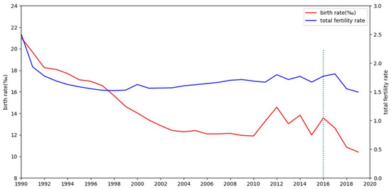
Figure 1.
Changes in China’s birth rate and total fertility rate from 1990 to 2019 (to avoid the impact of the COVID-19 pandemic, data from the year 2020 and beyond are not presented). Data source: China Statistical Yearbook and World Bank; Software: Python 3.10.
In response to the continuous decline in the fertility rate, China implemented the “conditional two-child” policy in 2014. This was followed by the “universal two-child” policy (UTCP) on 1 January 2016, which permits all families to have up to two children. As illustrated in Figure 1, the birth rate (birth rate is the ratio of the number of births to the average population in an area over a period of time (usually one year). It is used to reflect the level of population birth and is generally expressed in thousandths) increased significantly in 2016 and 2017, reaching 13.57‰ and 12.64‰ from 11.99‰ in 2015. These data suggest that the implementation of the UTCP has an impact on the size and structure of Chinese families by changing the number of children in a family, which will influence the economic and financial behavior of families.
Financial asset allocation is an important economic activity for households and a proper allocation of financial assets will enable households to earn more property income and facilitate the appropriate allocation of social capital [3]. Despite the increasing depth and breadth of household participation in China’s financial market in recent years, the overall participation rate and the diversity of financial products held remain relatively low. Statistics indicate that most households primarily hold risk-free financial assets such as cash and deposits, leading to a “limited participation puzzle” in the stock market. For instance, in 2019, the proportions of holding stocks, funds, and bonds were 4.4%, 1.3%, and 0.2%, respectively, and 70.5% of households with risky assets held only one type of financial product. In contrast, the corresponding proportions for American households were 15.2%, 9.0%, 8.6%, and 48.31%. Household financial asset allocation behavior not only determines the living standard and wealth accumulation of households at the micro level but also affects the vitality of the financial market at the macro level, thereby affecting social welfare and the long-term sustainable development of the society and economy. The impact of the implementation of the UTCP on household risk asset holdings, the underlying impact mechanism, and the differential impact based on various household characteristics are critical areas of this study. Understanding these aspects will shed light on how the relaxation of fertility policy affects the development of the financial market. To systematically assess the influence of fertility or fertility expectation on household financial asset allocation, we use the implementation of the UTCP in China as an exogenous shock to construct a difference-in-difference (DID) model for estimation, based on the China Family Panel Studies (CFPS) data from 2010 to 2018. Our findings indicate that the policy implementation has a significant negative impact on the risk assets holdings. Specifically, the policy reduces the probability of participating in the financial market by 3.1 percentage points, which is equivalent to 47.2% of the sample mean. Additionally, the policy leads to a 50.2% decrease in the total value of risk assets held and a 1.76 percentage points reduction in the proportion of risk asset investment, which is equivalent to 70.1% of the sample mean.
Our analysis of the mechanism is conducted from two perspectives. Firstly, we find that the implementation of the policy has a significantly negative impact on labor market outcomes for women, as confirmed in the literature [4,5]. This leads to a reduction in household income and consequently, a decrease in resources available for financial asset allocation, which results in a negative impact on financial market participation and risk asset investment. Secondly, the policy notably increases the time and effort households spend on childcare, which squeezes out the time available for gathering information and conducting financial asset transactions, further affecting household investment in risk assets [6].
Rich heterogeneity by household characteristics is discussed. First of all, considering the differences in income stability [7,8], based on the wife’s employment status in 2014, the sample is divided into “households with wife-employed” sub-sample and “households with wife-self-employed” sub-sample. We only find the UTCP significantly reduces the risk asset holdings for the “households with wife-self-employed” sub-sample. Further investigation finds that total household income declines more for the “households with wife-self-employed” sub-sample compared with the “households with wife-employed” sub-sample, indicating that the instability income is the reason for the decrease in risk asset holdings for these sub-samples. Secondly, considering the time and effort spent on childcare [8], which will squeeze out the time available for gathering information and conducting financial asset transactions, we divide the sample according to whether the households co-reside with grandparents in 2014. The results show that the policy does not have a significant impact on the financial asset investment decisions for households co-residing with grandparents, and has a significant negative impact on the risk asset investment for households not co-residing with grandparents. The former can receive help from the grandparents, greatly reducing the time spent by the couple on childcare and housework, so that household risk asset holdings are not significantly affected. Finally, we divide the sample into “high-income households” and “low-income households” based on whether the annual household income is above the sample mean in 2014. The results show that the implementation of the policy significantly reduces the total value of risk assets held for high-income households, and low-income households are not significantly affected. This may be because high-income households have a more aggressive response to the policy, leading to a significant reduction in their risk asset holdings.
This paper contributes to the literature in the following aspects. Firstly, in the literature, while scholars have pointed out that family structure and the number of children are important factors related to household financial asset allocation, the results are mixed [9,10,11,12,13,14]. Large studies deem that the increase in children number will have a significant impact on risk asset holdings, but little attention is paid to the situation in China. Our study provides further evidence to evaluate the impact of the number of children and household fertility decisions on risk asset holdings. The results show that the increase in the number of children will have a significantly negative effect on risk asset holdings, which is consistent with the studies of Loayza et al. (2000) [9], Kang and Hu (2021) [10], and so on. Furthermore, we focus on the intention effect, which not only includes the direct effect of having more children, but also the expectation effect. Secondly, given China’s vast population and status as the country with the largest elderly population, changes in China’s fertility policy will have profound impacts both domestically and globally. In addition to the impact of China’s fertility policy on sex ratio [15,16], population structure and economy [17], outcomes [18], labor supply [19], and household debt [20], our study combines fertility policy with a new field—household financial asset allocation decision, which greatly enriches the research on this topic. Both fertility policy and household financial asset allocation are important topics that affect sustainable economic development, and numerous studies have also established a close link between financial development and subsequent economic growth [21,22]. By a detailed mechanism analysis from the perspectives of household income, expenditure, and time and effort invested in childcare, we demonstrate the incompleteness of supporting measures for fertility policies in developing countries and its negative effect on financial market, which provides reference for further optimizing fertility policies.
The rest of this article is structured as follows. Section 2 provides a review of the relevant literature, followed by a description of data and variables in Section 3; Section 4 delves into the identification strategy and regression results; Section 5 conducts a mechanism analysis and Section 6 presents the results of heterogeneity analysis; Section 7 is dedicated to robustness tests; Section 8 includes the limitation and discussion; and Section 9 concludes and gives the suggestion.
2. Literature Review and Hypothesis
A large literature has extensively discussed the factors influencing the total amount and structure of household financial asset allocation. Those factors include demographic characteristics, like gender, age, education, income, and wealth [23,24,25,26,27], risk attitudes and background risks [28,29,30,31,32,33], and financial literacy and cognitive ability [34,35,36,37]. Factors like social capital [38,39,40] and social security policies [41,42] also have an impact on household financial asset allocation.
The adjustment of fertility policy will change the population size and structure of a family. For example, Ge and Shi (2023) finds that the implementation of UTCP significantly increased the possibility of having children [43]. And empirical evidence has long acknowledged that family size and structure are important factors in household financial asset decisions. Little studies deem that a larger family size or more children will increase the holding of risky assets in a specific period or condition For example, Love (2009) indicates that earlier in the life cycle, households with children hold riskier portfolio shares (by about 10 percentage points) than households without children, but the relationship reverses in retirement [13]. Bogan (2015) shows that the expectation of preparing expenses for children’s college education will increase the holding of risky assets in the current period to achieve wealth appreciation and smooth consumption [14]. Most scholars deem that a larger family size or more children will decrease the holding of risky assets. For example, Loayza et al. (2000) points out that the birth of a child can change the household’s consumption structure and savings level [9]. To ensure the life quality of the new child, the household’s consumption expenditure level will increase to a certain extent, which will reduce the household’s willingness to invest. Kang and Hu (2021) reaches a similar conclusion, stating that as the promotion of infants increases, the probability and proportion of household holding risk assets decrease [10]. Calvet et al. (2014) finds that larger households tend to choose conservative investment portfolios (lower proportion of risky assets in household wealth) because the number of adults and children reduces per capita wealth and the larger households have higher expenditure-wealth ratios and need to bear the risks brought about by the random demands of a large number of family members [11]. These effects encourage larger households to adopt prudent asset allocation. Raurich and Seegmuller (2019) concludes that households’ investment in their own education (human capital) is negatively related to the number of children individuals will have by establishing a savings-economic growth model [12], indicating that more children means more upbringing costs, which will have a certain crowding out effect on household risk asset investment. Meanwhile, theoretically, according to the life cycle theory of savings, in the younger stage, income is lower, the cost of raising children is higher, and household savings are lower in China [44]. As a part of savings, risk asset investment will also decrease due to an increase in the number of children. Based on the theoretical and empirical analysis, we propose the following hypothesis:
Hypothesis 1:
The UTCP will reduce the households’ risk asset holdings.
In addition, we can obtain some inspiration from the literature about how fertility policy affects labor market outcomes. Fertility is an important factor affecting women’s career development [6,45], and the increase in fertility rates has led to an unprecedented increase in conflicts between fertility and career development faced by women [46]. One is the direct effect of the coming of a new child. Cao (2019) finds the one-and-a-half-child policy reduces material labor supply in rural China [19], and Huang and Jin (2022) finds that the UTCP has significantly reduced women’s employment by 4.06% and reduced their labor income by 10.43% [47]. The other is the indirect or expected effect, which is the discrimination for expected family responsibilities, even though not having a new child. He et al. (2023) finds that after the implementation of UTCP, women are subject to labor market discrimination for their expected family responsibilities, and this discrimination works as the probability of material increases with age for women [48]. In summary, the increase in fertility leads to an increase in unemployment and income risk for women. Therefore, the fertility policy relaxation may put households exposed to the risk of declining labor income, which may reduce the resources available for financial asset allocation and directly lead to a decrease in risk asset holdings. Based on the analysis above, we propose the following hypothesis:
Hypothesis 2:
The UTCP will reduce the households’ risk asset holdings by affecting household labor income.
Further, it is a common view that taking care of babies requires a lot of time and effort, which may lead to a decreasing ability/desire to keep up with the latest news in the financial market and master the latest technologies [6]. An example is that the life cycle model of fertility and career choice considers that mothers derive utility over child quality, which is produced with parental time inputs. It explains the “motherhood penalty” by women moving to lower-paid jobs that are closer to home after having an infant, which proves that more time is needed to care for babies [49]. Wu (2022) suggests the maternal labor supply declines after the implementation of UTCP, and the reasons are that mothers have to spend more time taking care of children and the childcare provided by formal institutions is rare for children younger than three years old in China [50]. However, participating in the financial market is also a time-dependent activity. Over the past decade, the limited stock market participation puzzle has received a lot of attention in the literature, and one of its prevailing explanations is the existence of stock market participation costs. These costs include the time and effort necessary for updating financial knowledge and information, following the current trends in financial markets, determining the optimal portfolio, and so on [51,52,53]. Given the total time in one day is fixed, the time and effort spent on childcare may have a crowding-out effect on household risk asset investment. Therefore, we propose the following hypothesis:
Hypothesis 3:
The UTCP increases the time and effort spent on taking care of children, thus squeezing out time for financial asset allocation decisions and reducing household risk asset holdings.
3. Data and Variables
The data used in this study are from China Family Panel Studies (CFPS), which were conducted by the China Social Science Survey Center of Peking University and cover 25 provinces (autonomous regions, and municipalities directly under the central government) in mainland China, excluding Tibet, Qinghai, Ningxia, Xinjiang, and Inner Mongolia. Hence, the data are nationally representative. Detailed allocation of various household financial assets is included, making it suitable for our research. The data began in 2010, and the survey is conducted every two years. In our study, we used data from 2010 to 2018.
The universal two-child policy (UTCP), officially implemented on 1 January 2016, allows any couple to have two children. Before the UTCP, China introduced the “conditional two-child policy” in 2014, which means that couples could have two children if one of the parents is a single child. Therefore, the UTCP actually relaxes the birth restrictions for households where both spouses were not an only child, but has no effect on households where at least one of the spouses was an only child. We take households where both spouses were not an only child as the treatment group and households where at least one spouse was an only child as the control group to construct a DID model to evaluate the differences in household financial asset allocation between the two groups before and after the implementation of UTCP in 2016. The sample is limited to households where the wife was between 20 and 40 years old in 2016. The reason for restricting the sample based on the wife’s age rather than the husband’s age is that the wife’s age and physical condition directly determine whether the child can be born healthily; in contrast, the husband’s influence is relatively small. Meanwhile, the legal marriage age for women is 20 years in China, and the fertility of women tends to decline after the age of 40. In the robustness test, we further relax the upper limit of the wife’s age from 40 to 50 years old in 2016 year by year, and the results remain significantly negative. After dropping observations with missing key variables, our sample includes 5205 observations.
Part A of Table 1 presents the descriptive statistics for outcome variables. The outcome variables characterize various aspects of household risk asset holdings, including whether to participate in the financial market (”risk_asset”), which measures the extensive margin of household risk asset holdings, the total value of risk assets held (”ltotal_value”), and the proportion of risk asset investment (”risk_ratio”), which together measure the intensive margin of household risk asset holdings. Specifically, we define households holding one or more financial products (stocks, bonds, funds, trust products, and foreign exchange products) as participation in the financial market, and in this case, the variable “risk_asset” equals 1. If a household does not hold any of these financial assets, the variable “risk_asset” equals 0. As can be observed in Table 1, only 6.6% of the households in the sample participate in the financial market, indicating that overall, there is further room for improvement in the level of financial market participation. The variable “ltotal_value” represents the total value of risk assets held and is expressed as the logarithm of the sum of the total value of risk assets held plus one. Therefore, if a household does not hold any risk assets, i.e., does not participate in the financial market, then the variable equals 0. The variable “risk_ratio” refers to the proportion of the total value of risk assets held in the total value of all financial assets. It is calculated by dividing the total risk asset value by the sum of the total financial asset value plus one, where the financial assets consist of risk assets, cash, bank deposits, and money lent to others. The reason for adding one to the denominator is that some households may have no financial asset, resulting in a total risk asset value of 0 as well. In this case, directly dividing the total risk asset value by the total financial asset value would lead to missing data for those households. By adding one to the denominator, the value ”risk_ratio” for those households becomes 0, and we can keep more observations. On average, the proportion of risk asset investment in the sample is only 2.5%, indicating that households do not allocate much of their funds to the financial market.

Table 1.
Summary statistics.
In the Part B of Table 1, the variable “treat” indicates whether the household is a treatment group, which equals 1 if both spouses were not an only child, and 0 if at least one spouse was an only child. As the UTCP was officially implemented on 1 January 2016, the variable “post” represents whether the period is after the implementation of the policy, which equals 1 for years in and after 2016, and 0 for years before 2016.
The variables used in the mechanism analysis are shown in Part C of Table 1. Total household income (”ltotal_income”) consists of wage income, operating income, transfer income, property income, and other household income. Total household expenditure (”lexpense”) refers to the sum of consumption expenditure, transfer expenditure, security expenditure, and housing-related loan expenditure, with consumption expenditure (”lconsume_exp”) including expenses on food, clothing, housing, household equipment and daily necessities, transportation and communication, culture, education and entertainment, health and medical care, and other consumer-related expenses. Similarly, to keep more observations in the regression analysis, we add 1 to the above variables when taking the logarithm, in case it becomes missing data when directly taking the logarithm with a value of 0.
Variables related to time allocation include (1) housework time, “housework_w_wife” and “housework_w_hus” represent the average weekly time spent by the wife and husband on housework, respectively. The average weekly time spent doing the housework by wives is 17.80 h, which is much higher than the 8.86 h spent by husbands. This aligns with the traditional Chinese philosophy of “men are responsible for external affairs while women are responsible for internal affairs”; and (2) sleep time, “sleep_w_wife” and “sleep_w_hus” represent the average weekly sleep time of wife and husband, respectively. The average weekly sleep time for wives is 55.85 h, which is close to 54.64 h for husbands.
Variables used in the heterogeneity analysis include: (1) whether the wife was employed by others in 2014, (2) whether the household co-resided with grandparents in 2014, and (3) whether the household had a high income (higher than the sample average) in 2014. The statistics show that 39.8% of households with wife’s work employed by others, 39.4% of households co-resided with grandparents, and 53.5% of households were high-income households.
4. Identification Strategy and Regression Results
4.1. Empirical Strategy
We use the DID method to evaluate the impact of the UTCP on household risk asset holdings. In reference to Ge and Shi (2023) [43], the regression model is as follows:
where
and
represents the household, represents the year, and represents the province where the household is located. is the explained variable, including whether to participate in the financial market (risk_asset), the total value of risk assets held (ltotal_value), and the proportion of risk asset investment (risk_ratio). indicates whether the household is a treatment group, which equals 1 if both spouses in the household were not an only child, and equals 0 if at least one spouse in the household was an only child. represents whether the period is after the implementation of the policy, which equals 1 for years in and after 2016, and 0 for years before 2016. represents the household fixed effects, which control for the time-invariant and household-level unobserved variables, and represents the year-fixed effects. The household-year level variables include the ages of the wife and the husband. We do not control for other variables at the household-year level (such as education level, income level, and employment status of the couple) because: (1) variables that change with the household but do not change with time (such as education level, ethnic identity of a couple) have been controlled by the household fixed effect . (2) variables that change with time but do not change with the household have been controlled by the year-fixed effect. (3) if we control variables that are not determined before the implementation of the policy, they may be affected by the policy (such as income level, and employment status of the couple). Including these variables in the regression equation could introduce bias in the estimation results because they are bad controls proposed in Angrist and Pischke (2009) [54].
The variables and are perfectly collinear with and respectively, therefore, they cannot be included in the regression equation. To further control for the influence of changes in economic and social factors across different provinces on household risk asset holdings, we include the interactions between the linear term of the survey year and the province dummy variable, in the regression. represents the error term. Considering that disturbance terms of households within the same county may be correlated, this study clusters the regression standard errors at the county level.
is the coefficient of interest, which reflects the impact of the universal two-child policy on household risk asset holdings.
4.2. Baseline Results
Table 2 presents the regression results for the implementation of the UTCP on household risk asset holdings. Columns (1), (3), and (5) do not include the cross-term of the linear trend of year and the province dummy, while Columns (2), (4), and (6) include it. The results indicate that the policy implementation has a significantly negative impact on household risk asset holdings. Specifically, after the implementation of the UTCP, compared with the control group, the probability of participating in the financial market in the treatment group decrease by 3.1 percentage points, which is equivalent to 47.2% of the sample mean (0.0311/0.0659 × 100% = 47.2%), and the coefficient is significant at the 5% level. It measures the extensive margin of household risk asset holdings, and it is a big negative effect, compared with the sample mean. Meanwhile, the impact to the intensive margin of household risk asset holdings is also significant. The policy results in a 50.2% decrease in the total value of risk assets, and the coefficient is significant at the 1% level. Additionally, the policy reduces the proportion of risk asset investment by 1.76 percentage points, which is equivalent to 70.1% of the sample mean (0.0176/0.0251 × 100% = 70.1%), and the coefficient is significant at the 10% level. Overall, the implementation of the UTCP has a significant negative impact on household risk asset holdings.
Table 2.
The effect of the UTCP on household risk asset holdings.
The above discussion validates Hypothesis 1.
4.3. Parallel Trend Test
In this section, we show the results of the parallel trend test. The prerequisite for the validity of the DID model is that the parallel trend test needs to be satisfied, that is, the trends of the outcome variables in the control group and the treatment group should be consistent before the implementation of the UTCP. Similar to Keiser and Shapori (2019) [55] and Zhang and Zheng (2023) [56], we use an event study to verify it, and the regression model (1) is modified as follows:
The variable in Model (1) is replaced by the dummy variable for a range of survey years, where s is the survey year, taking the values of 2010, 2012, 2016, and 2018. Since the UTCP was implemented on 1 January 2016, the most recent year before policy implementation, i.e., 2014, is taken as the base year, the dummy variable for the year 2014 is removed, and the dummy variables for other years are multiplied by . The dummy variable for the survey year, , is not included in regression Equation (2) because they are completely collinear with and cannot be added to the regression.
Figure 2 shows the estimated coefficients of along with its 95% confidence intervals. Findings confirm that before the implementation of the policy, the coefficients are not significantly different from 0, indicating that we cannot reject the null hypothesis and that the treatment and control groups have the same trend of risk asset holdings before the UTCP. Only after the implementation of the policy was there a significant difference between the treatment and control group, which validates the parallel trend assumption is valid.
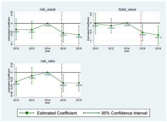
Figure 2.
Parallel trend test; Software: Stata 15.
In addition, the dynamic results show that the absolute values of the coefficients for the first two dependent variables in 2018 are greater than the corresponding values in 2016. This may be because the UTCP was implemented on 1 January 2016, and fewer households were affected by the policy in 2016, so the impact on financial asset allocation was not as great as that in 2018.
5. Mechanism Analysis
The baseline results show that the implementation of the UTCP reduces the probability of participating in the financial market as well as the total amount and proportion of risk assets held. In this section, we explore what causes the decrease in risk asset holdings.
5.1. Household Income and Household Expenditure
First, risk asset holdings, as an investment decision, is closely related to household budget constraints. If household income decreases or household expenditure increases, the resources available for investment will decline, and risk asset holdings may be affected. Large literature shows that fertility may have an impact on household income and expenditure. On one hand, the fertility behavior may lead to an unprecedented increase in conflicts between fertility and career development faced by women, which puts women in a disadvantaged position in the labor market, resulting in lower wages, reduced working hours, and increased unemployment [4,5,46] On the other hand, to ensure the life quality of the new child, the household’s consumption expenditure level will increase to a certain extent (Loayza et al., 2000) [9]. Therefore, we first analyze the impact of the UTCP on household income and household expenditure.
The outcome variables in Equation (1) are changed to variables representing total household income and household expenditure for regression, and the regression results are shown in Table 3. To save space, we only report the results after controlling for the linear trend of province × year. Column (1) reports the regression result for total household income. The UTCP significantly reduces total household income. On average, the policy reduces the total household income by 8.7%, and the coefficient is significant at the 5% level. The results are consistent with previous literature research. Columns (2) and (3) report the regression result for total household expenditure and consumption expenditure, respectively. The coefficients are both negative but insignificant. That is, we find the UTCP has a significant negative impact on total household income but does not have an impact on total household expenditure or consumption expenditure. The decrease in household income reduces the funds available for financial asset allocation, thereby reducing risk asset holdings.
Table 3.
The impact of the UTCP on household income and expenditure.
The above discussion validates Hypothesis 2.
5.2. Time Allocation
Apart from additional funds, time is also needed to gather information and conduct transactions for financial asset investment. The literature points out the existence of stock market participation costs, which include the time and effort necessary for updating financial knowledge and information, following the current trends in financial markets, determining the optimal portfolio, and so on [51,52,53]. Therefore, if the implementation of the UTCP affects the time allocation and changes the time input in financial asset investment, household financial asset allocation decisions will also be affected. Studies show that after an increase in fertility behavior, more time and effort is needed to take care of children [6,49,50], leading to an unprecedented increase in time pressure for families and less time and effort left for other activities (including finding information and trading stocks), which may lead to a reduction in household risk asset holdings. It would be perfect if we could test this channel by using the time spent in taking care of children. Unfortunately, the data used in this study do not have direct information on the time and effort spent on childcare. We choose the time spent on the housework and the sleep time as the proxy variable to measure the time and effort spent in caring for children because: (1) The time spent on the housework is available and it includes the time spent in preparing food, washing clothes, cleaning rooms and so on, which to some extent reflects the impact of taking care of children. (2) The sleep time is available and it is a consensus that taking care of a baby will sacrifice the sleep time of parents, especially mothers. (3) Furthermore, large literature has pointed out that intergenerational care can significantly lower young parents’ time in caring for children. In the following heterogeneity analysis, we find that the wife’s housework time for households not co-residing with grandparents significantly increase after the implementation of the UTCP, but it does not change significantly for households co-residing with grandparents, which indicates that it is reasonable to take the housework time as the proxy variable. Therefore, we use time spent in doing housework (We further investigated the impact of the UTCP on weekly main work hours and found that weekly main work hours of wife or husband did not significantly decrease after the policy was implemented, which means that the increase in housework time is not caused by the decrease in main work hours) to measure the impact of the UTCP on the time spent in caring for children and uses the sleep time to measure the impact of the policy on the effort spent on childcare.
- 1.
- The impact on time spent in caring for children: using housework time as a proxy variable
Columns (1) to (3) of Table 4 report the regression results for the impact of the UTCP on housework time. On average, compared with the control group, after the policy, the wife’s weekly housework time in the treatment group increases by 1.43 h, which is equivalent to 8.1% of the sample mean, and the coefficient is significant at the 10% level. The husband’s weekly housework time in the treatment group also increases, but the coefficient is small and not statistically significant. The total weekly housework time of the wife and husband is positive and insignificant, too. Overall, the results indicate that the implementation of the policy significantly affects wives’ weekly housework time, which, in turn, leads to a significant reduction in the time available for other activities.
Table 4.
The impact of the UTCP on housework time and sleep time.
- 2.
- The impact on effort caring for children: using sleep time as a proxy variable
We use sleep time as a proxy variable to measure the effort spent in caring for children. If the sleep time of household members decreases after the UTCP is implemented, it can be considered that caring for children takes more effort for household members (We do not believe that the following is logical: A reduction in sleep time implies more time for information gathering and thus a positive impact on household risk asset holdings). The regression results in columns (4) and (5) of Table 4 show that compared with the control group, after the policy, the wife’s sleep time in the treatment group significantly decreases. Specifically, the wife’s weekly sleep time decreases by 1.61 h on average, with the coefficient significant at the 5% level; and the impact on the husbands’ sleep time is insignificant. Therefore, it can be inferred that after the policy implementation, household members need to spend more time and effort on their children, reducing their time and effort devoted to other activities, especially investment, which requires more effort, thus significantly decreasing household risk asset holdings.
The above discussion validates Hypothesis 3.
6. Heterogeneity Analysis
The above analysis shows that after the implementation of the UTCP, the reduction in household income and the increased time and effort spent in caring for children are the reasons for the significant reduction in household risk asset holdings. However, different types of households may be affected differently in terms of household income, time, and effort, and thus, the degree of impact on household risk asset holdings may also vary. In this section, we analyze the heterogeneity impacts of the UTCP on different households.
6.1. Households with Wife Employed by Others versus Households with Wife Self-Employed
First, the type of work is related to the stability of household income. Self-employment work is more dependent on the input of time [57], whose income has more instability [58], and is often accompanied by a lack of social security [59]. Comprehensive social security is also an important factor affecting the risk assets holdings. When residents have one or more types of insurance, the uncertainty of future protective expenditures will be reduced, leading households to lean towards investing in risky financial assets [60,61]. Yener (2020) also finds that the deeper the investment depth of insurance, the wider the coverage of life security, and the higher the investment rate of households in risky financial assets such as stocks [62]. Therefore, we divide the sample into the “households with wife employed by others” sub-sample and “households with wife self-employed” sub-sample according to the wife’s employment type in the year 2014 to explore the heterogeneous impact of the UTCP on household risk asset holdings. The reasons for using the wife’s employment in 2014 are as follows: (1) women’s employment status and income are more likely to be affected during the process of pregnancy and caring for a child [7,8]. (2) by using data from 2014, it can be ensured that this variable is not affected by the implementation of the UTCP, thereby ensuring the exogenous of the control variables.
Part A and Part B of Table 5 show the regression results for the sub-samples of households with wife employed by others and self-employed, respectively. To save space, the results after controlling for the linear trend of province × year are presented. The regression results show that for the sub-sample of households with wife employed by others, the impact of the UTCP on the household risk asset holdings is negative but not statistically significant. In contrast, for the sub-sample of households with wife self-employed, on average, the UTCP reduces the probability of household participation in the financial market by 4.5 percentage points, equivalent to 2.23 times the sample mean (0.0445/0.020 = 2.23), with the coefficient significant at the 5% level; the total risk assets held decrease by 56.4%, with the coefficient significant at the 5% level; and the proportion of the total risk assets held in financial assets decreases by 3.41 percentage points, which is 4.26 times the sample mean (0.0341/0.008 = 4.26), with the coefficient significant at the 1% level. In summary, for the sample of households with wife self-employed, the UTCP significantly reduces household risk asset holdings.
Table 5.
The heterogeneous effect of the UTCP on households with wife’s different employment status.
Furthermore, we regress the total household income of the sub-samples, and the results are shown in Column (4). The total household income decreases significantly for both sub-samples, but the decline level is higher for households with wife self-employed than for households with wife employed by others. On the one hand, this may be due to the higher dependence on personal labor and time for the source of income for households with wives self-employed, which makes the impact of having or expecting to have a child on total household income greater (with a coefficient of −0.2145) and furthermore reduces the amount of household funds available for investment, thus reducing risk asset holdings. On the other hand, the risk preference may make sense because of the inherent greater volatility of income from self-employment compared to employed work. When taking into account the demand for cash flow for the various costs of raising children and the higher risk and uncertainty of investing in risk assets, households with wife self-employed reduce their risk asset holdings. For households with wife employed by others, although the total household income also decreases significantly, it does not affect household risk asset allocation decisions, probably because they have more comprehensive social security and the income is more stable.
6.2. Households Co-Residing versus Not Co-Residing with Grandparents
Next, we divide the sample according to whether households co-resided with grandparents in 2014. The previous findings suggest that more time and effort spent in caring for children is one of the reasons for the significant reduction in household risk asset holdings. A large literature has pointed out that intergenerational care can significantly lower young parents’ time in caring for children. Battistin et al. (2014) shows that delayed retirement has a negative impact on the fertility rate of young parents, mainly due to the fact that paternal retirement can increase the supply of care or time spent caring for grandchildren [63]. Based on research in the Chinese context, Maurer-Fazio et al. (2011) finds that when daughters live with their parents or parents-in-law, their labor force participation rate can increase by 12 percentage points, illustrating the positive role of intergenerational caregiving [64]. Li et al. (2015) also points out that the negative impact of fertility on parental labor supply can be alleviated through parenting services provided by grandparents [65]. Therefore, for households co-residing with grandparents, help from old people can greatly reduce the time spent by a couple on childcare and housework, thus making household financial asset allocation decisions different from those of households not co-residing with grandparents. To verify this conclusion, we regress the sub-samples divided by whether households co-resided with grandparents in 2014. The detailed regression results are presented in Table 6.
Table 6.
The heterogeneous effect of the UTCP on households that co-reside and do not co-reside with grandparents.
Part A and Part B of Table 6 show the regression results for the sub-samples of households co-residing with grandparents and households not co-residing with grandparents, respectively. For households co-residing with grandparents, the UTCP has no significant negative impact on risk asset holdings. In contrast, for households not co-residing with grandparents, on average, the policy leads to a 6.7 percentage point decrease in the probability of participating in the financial market, which is equivalent to 87.3% of the sample mean (0.0666/0.0763 = 0.8729), with the coefficient significant at the 1% level; the total risk assets held decrease by 98.5%, with the coefficient significant at the 1% level; and the risk assets proportion decreases by 4.4 percentage points, equal to 1.42 times the sample mean (0.0437/0.0308 = 1.4188), with the coefficient significant at the 5% level. The regression results show that only the risk asset holdings for households not co-residing with grandparents will be affected by the UTCP.
As we demonstrated in Hypothesis 3, the time and effort spent on childcare have a crowding-out effect on household risk asset investment. Therefore, only if we find that the time spent on housework for households not co-residing with grandparents increases after the UTCP, can we verify the validity of this hypothesis. Further, we regress the housework time and sleep time on the policy for each of the sub-samples, and the results are shown in Table 7. For households that co-reside with grandparents, neither the wife’s weekly housework time, the husband’s weekly housework time nor the total weekly housework time of the wife and husband is significant. The wife’s weekly sleep time decreases by an average of 2.32 h, with the coefficient significant at the 10% level, and the impact on the husband’s sleep time is not significant. In contrast, for households that do not co-reside with grandparents, the wife’s weekly housework time on average increases by 2.37 h, and the total weekly housework time increases by 2.66 h, with coefficients significant at the 10% level. The wife’s weekly sleep time decreases by 2.58 h, with the coefficients significant at the 10% level; and the impact on the husband’s sleep time is not significant. Overall, the results verify the validity of Hypothesis 3: households not co-residing with grandparents spend more time and effort on childcare after the implementation of the UTCP and accordingly spend less time on information gathering and financial asset investment, thereby negatively impacting risk asset holdings.
Table 7.
The heterogeneous effect of the UTCP on households co-residing and not co-residing with grandparents—weekly housework time and sleep time.
6.3. High-Income Households versus Low-Income Households
Finally, considering that households with different income may respond to the policy differently, we divide the households into “high-income households” and “low-income households” based on whether the annual household income in 2014 was higher than the sample average. The results are shown in Table 8.
Table 8.
The heterogeneous effect of the UTCP on high-income households versus low-income households.
The regression results show that the implementation of the policy causes the total value of risk assets held by high-income households to decrease by 50.7% but does not have a significant impact on risk asset holdings for low-income households. Furthermore, the total household income of high-income households decreased by 17.88% after the implementation of the policy, but it does not change significantly for low-income households. Considering the high cost of raising children, high-income households may have a more aggressive respond to the policy, leading to a significant reduction in their risk asset holdings.
7. Robustness Tests
7.1. Placebo Tests
The baseline results show that the UTCP has a significant negative impact on household risk assets holdings, but the above results still cannot rule out the possible role of other factors. Therefore, we perform a series of placebo tests to rule out the bias induced by omitted variables.
- 1.
- Regression using a sample of rural households
During the one-child policy period, not all households were limited to having only one child. For rural residents, families in which both spouses were rural residents and their first child was a girl could have a second child. Therefore, these rural households could have two children before the implementation of the UTCP, and thus, their household financial asset allocation decision should not change due to the implementation of the UTCP. That is, if there were no unobserved omitted variables, we expect the risk asset holdings would not be affected by the policy for rural households.
We manually obtain the requirement on the birth of a second child for rural residents in each province (in the early years of the implementation of the one-child policy, each province (municipality directly under the central government/autonomous region) had the following regulations on the birth of a second child for rural residents: (1) In 17 provinces (autonomous regions), namely Hebei, Shanxi, Inner Mongolia, Jilin, Hei-longjiang, Zhejiang, Anhui, Fujian, Jiangxi, Henan, Hubei, Hunan, Guangdong, Guizhou, Shaanxi, Gansu, and Qinghai, families in which the husband and wife were both rural residents and the first child was a girl were allowed to have a second child; (2) In three provinces (autonomous regions), namely Liaoning, Shan-dong, and Guangxi, a family in which the wife was a rural resident and the first child was a girl was allowed to have a second child; (3) In Yunnan, families in which one of the spouses was a rural resident were allowed to have a second child; and (4) In Xinjiang and Ningxia, families in which both spouses are rural residents may have a second child) and obtain a restricted sample of rural households with a sample size of 1759. The regression results using this sub-sample are shown in part A of Table 9. After controlling for the household fixed effects, survey year fixed effects, ages of the husband and wife, and the linear trend of province × survey year, none of the three outcome variables are significant, indicating that the UTCP has no impact on the household risk asset holdings of this group.
Table 9.
Placebo test using sample unaffected by the UTCP.
- 2.
- Households with two or more children before the policy implementation
In Part B of Table 9, we conduct a regression using a sample that only includes households that already had two or more children before the implementation of the UTCP. We find that these households do not respond significantly to the policy, which is again consistent with our expectations.
- 3.
- Regression with a falsified policy implementation time
Finally, we conduct a falsified policy implementation time analysis by assuming that the policy was implemented in early 2012 or early 2014. We estimate the policy effect using only the sample before the implementation of the UTCP. Since there was no policy implemented at that time, we expect the interaction terms of the falsified policy indicator to have no impact on households risk asset holdings. The results are shown in Table 10. The coefficients of the interaction terms in this case are not significant. Combining the results of the placebo tests above, we are confident in believing that the findings obtained in this study are indeed a result of the impact of the UTCP implemented in 2016.
Table 10.
Placebo test with a falsified policy implementation time.
7.2. Permutation Test
Figure 3 reports the results of the permutation test for the three outcome variables. We randomly assign each household in the sample to the treatment group and the control group, and then estimate the policy effect based on Equation (1). We repeat this exercise 2000 times. The distributions of the estimated policy effects on the three outcome variables are plotted in Figure 3. The dotted vertical line in the figure corresponds to the estimation results of the benchmark regression, and the P-value measures the proportion of the regression results from the 2000 regressions greater than benchmark regression results. The results show that none of the coefficients from the 2000 regressions exceed the coefficients from the benchmark regression (significant at the 1% level). Therefore, the findings of our study are not caused by random factors but are indeed the result of the impact of the UTCP.
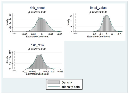
Figure 3.
Permutation test results; Software: Stata 15.
7.3. Regression Using Different Wife’s Age Samples in 2016
In the baseline regression, we restrict the sample to households whose wife were 20–40 years old in 2016. To show that the findings of our study are not affected by the specific age restriction, we relax the upper limit of the wife’s age from 40 years old to 50 years old year by year and conduct regression for each age sample using Equation (1). To save space, the results after controlling for the linear trend of province × year are presented. As shown in Table 11, the conclusions of this study do not change after the wife’s age is relaxed, and the UTCP still has a significant negative impact on risk asset holdings. Comparing the regression coefficients, we can find the absolute values of the coefficients decrease with the increase of the upper limit of the wife’s age. This may be because households with older wife are less inclined to have a second child and therefore household financial asset allocation decisions are less impacted.
Table 11.
Regression results using different wife’s age samples in 2016.
7.4. Controlling for More Individual and Household Level Pre-Determined Variables in 2014
The control group used in our study is the household where at least one of the spouses was an only child, while the treatment group is the household where neither spouse was an only child. To further eliminate the differences between the treatment and control groups, we further controlled for a series of cross-terms between individual and household level variables in 2014, and the variable of . These variables include: whether the wife worked in 2014, whether the husband worked in 2014, whether the couple had their own house in 2014, the household income in 2014, the wife’s health status in 2014, and the husband’s health status in 2014. By using data on the above variables in 2014, it can be ensured that these control variables are not affected by the implementation of the UTCP, thereby ensuring the exogenous of the control variables. And considering that the data of these variables are fixed in 2014 and will be absorbed by the household fixed effect if directly included in the regression, we multiply these variables with the variable . The corresponding regression results are shown in Table 12, and we can find the main results still be robust.
Table 12.
Regression results controlling for a series of cross-terms between individual and household level variables in 2014 and the variable of .
8. Limitation and Discussion
Although we have conducted a detailed analysis, there are still some areas that are worth exploring. One is the impact of children’s gender. Wei and Zhang (2011) proposes for the first time the concept of “competitive savings” to explain the rising savings rate of Chinese residents [66]. With the imbalance of gender ratio, families with boys are facing increasing pressure in the marriage market, so they will increase savings to increase their bargaining power in the marriage market. This example indicates that households with boys need to prepare more funds to help their children start a new family. Therefore, facing the relaxation of fertility policy, households with boys and households with girls may have different fertility desire, which may have differenteffect on the risk assets holdings. Furthermore, changes in risk attitude after the policy may be one of the channels. However, due to data availability limitations, we are unable to explore these issues. Finally, it should be pointed out that our conclusion is only a short-term effect. In the long run, the existence of this negative impact depends on the effectiveness of the fertility policy. If households do not have a big response to the fertility policy, apart from the weakening of direct effects from the increase in children, the expected effect will also weaken because when employers find that the fertility policy is not working, they will change their expectations and decrease the reproductive discrimination against female employees.
9. Conclusions and Suggestions
This study uses 2010–2018 CFPS data to estimate the impact of the UTCP on household financial asset allocation decisions using the DID method. We find that the implementation of the policy has a significant negative impact on household risk asset holdings. Specifically, the policy reduces the probability of participating in the financial market by 3.1 percentage points, which is equivalent to 47.2% of the sample average; it reduces the total value of risk assets held by 50.2% and decreases the proportion of risk asset investment by 1.76 percentage points, equivalent to 70.1% of the sample mean. The results of the mechanism analysis show that the decline in total household income and spending more time and effort caring for children are the two reasons for the decline in household risk asset holdings. Heterogeneity analysis indicates that the risk asset holdings of households with wife self-employed and households not co-residing with grandparents are more significantly affected by the policy and that high-income households respond more positively to the policy.
Both fertility policy and the healthy development of financial markets are important topics for sustainable economic and social development. Participating in the stock market is an important way to increase household property income, and diversified asset allocation has a positive effect on risk avoidance and long-term wealth accumulation for household total assets [14]. The purpose of relaxing the fertility policy is to increase the fertility rate, but our study finds that it has a negative effect on the labor market outcomes for women and household property income, which is not conducive to the long-term implementation of the policy. If related supporting policies are not introduced, it could reduce the effectiveness of fertility policies aimed at increasing birth rates. Simultaneously, it could negatively impact other household decisions, such as the household risk asset allocation studied in this paper, thereby reducing overall social welfare and the sustainability of economic development. Therefore, the government should vigorously introduce supporting policies in order to reduce the passive impact of households’ reproductive decisions on their financial asset allocation decision and achieve sustainable population growth. Policies aiming to improve employment security, enhance the household income level, establish a childcare welfare system, and ease the financial pressure on households to raise children may be effective.
Author Contributions
Conceptualization, Y.W. and R.G.; data curation, Y.W. and D.T.; formal analysis, Y.W.; funding acquisition, Y.W.; investigation, Y.W.; methodology, Y.W.; project administration, R.G.; software, Y.W. and W.G.; supervision, Y.W. and R.G.; validation, Y.W., R.G. and W.G.; visualization, Y.W. and R.G.; writing—original draft, Y.W.; writing—review and editing, Y.W. and W.G. All authors have read and agreed to the published version of the manuscript.
Funding
This research received no external funding.
Institutional Review Board Statement
Not applicable.
Informed Consent Statement
Not applicable.
Data Availability Statement
Publicly available datasets were analyzed in this study.
Conflicts of Interest
Author Yujie Wang was employed by the company Industrial and Commercial Bank of China. The remaining authors declare that the research was conducted in the absence of any commercial or financial relationships that could be construed as a potential conflict of interest.
References
- Bloom, D.E.; Canning, D.; Fink, G. Implications of population ageing for economic growth. Oxf. Rev. Econ. Policy 2010, 26, 583–612. [Google Scholar] [CrossRef]
- Liang, J.; Wang, H.; Lazear, E.P. Demographics and Entrepreneurship. J. Political Econ. 2018, 126, S140–S196. [Google Scholar] [CrossRef]
- Yuan, H.; Puah, C.H.; Yau, J.T. How Does Population Aging Impact Household Financial Asset Investment? Sustainability 2022, 14, 15021. [Google Scholar] [CrossRef]
- Jia, N.; Dong, X.-Y. Economic transition and the motherhood wage penalty in urban China: Investigation using panel data. Camb. J. Econ. 2012, 37, 819–843. [Google Scholar] [CrossRef]
- Killewald, A.; García-Manglano, J. Tethered lives: A couple-based perspective on the consequences of parenthood for time use, occupation, and wages. Soc. Sci. Res. 2016, 60, 266–282. [Google Scholar] [CrossRef] [PubMed]
- Kleven, H.; Landais, C.; Søgaard, J.E. Children and Gender Inequality: Evidence from Denmark. Am. Econ. J. Appl. Econ. 2019, 11, 181–209. [Google Scholar] [CrossRef]
- Greenhaus, J.H.; Beutell, N.J. Sources of Conflict Between Work and Family Roles. Acad. Manag. Rev. 1985, 10, 76–88. [Google Scholar] [CrossRef]
- Bauernschuster, S.; Schlotter, M. Public child care and mothers’ labor supply—Evidence from two quasi-experiments. J. Public Econ. 2015, 123, 1–16. [Google Scholar] [CrossRef]
- Loayza, N.; Schmidt-Hebbel, K.; Servén, L. Saving in Developing Countries: An Overview. World Bank Econ. Rev. 2000, 14, 393–414. [Google Scholar] [CrossRef]
- Kang, C.; Hu, R. Age structure of the population and the choice of household financial assets. Econ. Res. Ekon. Istraživanja 2022, 35, 2889–2905. [Google Scholar] [CrossRef]
- Calvet, L.E.; Sodini, P. Twin Picks: Disentangling the Determinants of Risk-Taking in Household Portfolios. J. Financ. 2014, 69, 867–906. [Google Scholar] [CrossRef]
- Raurich, X.; Seegmuller, T. Growth and bubbles: Investing in human capital versus having children. J. Math. Econ. 2019, 82, 150–159. [Google Scholar] [CrossRef]
- Love, D.A. The Effects of Marital Status and Children on Savings and Portfolio Choice. Rev. Financ. Stud. 2009, 23, 385–432. [Google Scholar] [CrossRef]
- Bogan, V.L. Household Asset Allocation, Offspring Education, and the Sandwich Generation. Am. Econ. Rev. 2015, 105, 611–615. [Google Scholar] [CrossRef]
- Ding, Q.J.; Hesketh, T. Family size, fertility preferences, and sex ratio in China in the era of the one child family policy: Results from national family planning and reproductive health survey. BMJ Clin. Res. Ed. 2006, 333, 371–373. [Google Scholar] [CrossRef]
- Zhou, Y. The Dual Demands: Gender Equity and Fertility Intentions After the One-Child Policy. J. Contemp. China Dang Dai Zhongguo 2018, 28, 367–384. [Google Scholar] [CrossRef]
- Huang, J.; Qin, D.; Jiang, T.; Wang, Y.; Feng, Z.; Zhai, J.; Cao, L.; Chao, Q.; Xu, X.; Wang, G.; et al. Effect of Fertility Policy Changes on the Population Structure and Economy of China: From the Perspective of the Shared Socioeconomic Pathways. Earth’s Future 2019, 7, 250–265. [Google Scholar] [CrossRef]
- Huang, W.; Lei, X.; Sun, A. Fertility Restrictions and Life Cycle Outcomes: Evidence from the One-Child Policy in China. Rev. Econ. Stat. 2021, 103, 694–710. [Google Scholar] [CrossRef]
- Cao, Y. Fertility and labor supply: Evidence from the One-Child Policy in China. Appl. Econ. 2019, 51, 889–910. [Google Scholar] [CrossRef]
- Deng, X.; Yu, M. Does the marginal child increase household debt?—Evidence from the new fertility policy in China. Int. Rev. Financ. Anal. 2021, 77, 101870. [Google Scholar] [CrossRef]
- Calvet, L.E.; Campbell, J.Y.; Sodini, P. Down or Out: Assessing the Welfare Costs of Household Investment Mistakes. J. Political Econ. 2007, 115, 707–747. [Google Scholar] [CrossRef]
- Levine, R. Financial Development and Economic Growth: Views and Agenda. J. Econ. Lit. 1997, 35, 688–726. [Google Scholar] [CrossRef]
- Mankiw, N.G.; Zeldes, S.P. The consumption of stockholders and nonstockholders. J. Financ. Econ. 1991, 29, 97–112. [Google Scholar] [CrossRef]
- King, M.A.; Leape, J.I. Wealth and portfolio composition: Theory and evidence. J. Public Econ. 1998, 69, 155–193. [Google Scholar] [CrossRef]
- Campbell, J.Y. Household Finance. J. Finance 2006, 61, 1553–1604. [Google Scholar] [CrossRef]
- Vaarmets, T.; Liivamägi, K.; Talpsepp, T. From academic abilities to occupation: What drives stock market participation? Emerg. Mark. Rev. 2019, 39, 83–100. [Google Scholar] [CrossRef]
- Dong, T.; Eugster, F.; Nilsson, H. Business school education, motivation, and young adults’ stock market participation. J. Account. Public Policy 2023, 42, 106958. [Google Scholar] [CrossRef]
- Grossman, S.J.; Laroque, G. Asset pricing and optimal portfolio choice in the presence of illiquid durable consumption goods. In National Bureau of Economic Research Cambridge; Cambridge University Press: Cambridge, UK, 1987. [Google Scholar] [CrossRef]
- Gollier, C.; Pratt, J.W. Risk Vulnerability and the Tempering Effect of Background Risk. Econometrica 1996, 64, 1109–1123. [Google Scholar] [CrossRef]
- Rosen, H.S.; Wu, S. Portfolio choice and health status. J. Financ. Econ. 2004, 72, 457–484. [Google Scholar] [CrossRef]
- Cocco, J.F. Portfolio Choice in the Presence of Housing. Rev. Financ. Stud. 2004, 18, 535–567. [Google Scholar] [CrossRef]
- Nadeem, M.A.; Qamar, M.A.J.; Nazir, M.S.; Ahmad, I.; Timoshin, A.; Shehzad, K. How Investors Attitudes Shape Stock Market Participation in the Presence of Financial Self-Efficacy. Front. Psychol. 2020, 11, 553351. [Google Scholar] [CrossRef] [PubMed]
- Niu, G.; Wang, Q.; Li, H.; Zhou, Y. Number of brothers, risk sharing, and stock market participation. J. Bank. Financ. 2020, 113, 105757. [Google Scholar] [CrossRef]
- Smith, J.P.; McArdle, J.J.; Willis, R. Financial Decision Making and Cognition in a Family Context. Econ. J. 2010, 120, F363–F380. [Google Scholar] [CrossRef]
- van Rooij, M.; Lusardi, A.; Alessie, R. Financial literacy and stock market participation. J. Financ. Econ. 2011, 101, 449–472. [Google Scholar] [CrossRef]
- Agarwal, S.; Mazumder, B. Cognitive Abilities and Household Financial Decision Making. Am. Econ. J. Appl. Econ. 2013, 5, 193–207. [Google Scholar] [CrossRef]
- Cheng, Y.-F.; Mutuc, E.B.; Tsai, F.-S.; Lu, K.-H.; Lin, C.-H. Social Capital and Stock Market Participation via Technologies: The Role of Households’ Risk Attitude and Cognitive Ability. Sustainability 2018, 10, 1904. [Google Scholar] [CrossRef]
- Hong, H.; Kubik, J.D.; Stein, J.C. Social Interaction and Stock-Market Participation. J. Financ. 2004, 59, 137–163. [Google Scholar] [CrossRef]
- Guiso, L.; Sapienza, P.; Zingales, L. Trusting the Stock Market. J. Financ. 2008, 63, 2557–2600. [Google Scholar] [CrossRef]
- Bricker, J.; Li, G. Credit Scores, Social Capital, and Stock Market Participation; Board of Governors of the Federal Reserve System: Washington, DC, USA, 2017. [Google Scholar] [CrossRef]
- Gomes, F.; Michaelides, A. Asset Pricing with Limited Risk Sharing and Heterogeneous Agents. Rev. Financ. Stud. 2008, 21, 415–449. [Google Scholar] [CrossRef]
- Ma, X. Social Insurances and Risky Financial Market Participation: Evidence from China. Emerg. Mark. Financ. Trade 2022, 58, 2957–2975. [Google Scholar] [CrossRef]
- Ge, R.; Shi, X. How does the universal two-child policy affect fertility behavior? China Econ. Q. Int. 2023, 3, 227–237. [Google Scholar] [CrossRef]
- Modigliani, F.; Cao, S.L. The Chinese Saving Puzzle and the Life-Cycle Hypothesis. J. Econ. Lit. 2004, 42, 145–170. [Google Scholar] [CrossRef]
- Lundborg, P.; Plug, E.; Rasmussen, A.W. Can Women Have Children and a Career? IV Evidence from IVF Treatments. Am. Econ. Rev. 2017, 107, 1611–1637. [Google Scholar] [CrossRef] [PubMed]
- Kilburn, M.; Datar, A. The Availability of Child Care Centers in China and Its Impact on Child Care and Maternal Work Decisions; RAND Corporation: Santa Monica, CA, USA, 2002; Available online: https://EconPapers.repec.org/RePEc:ran:wpaper:dru-2924-nih (accessed on 19 October 2023).
- Huang, Q.; Jin, X. The effect of the universal two-child policy on female labour market outcomes in China. Econ. Labour Relat. Rev. 2022, 33, 526–546. [Google Scholar] [CrossRef]
- He, H.; Li, S.X.; Han, Y. Labor Market Discrimination against Family Responsibilities: A Correspondence Study with Policy Change in China. J. Labor Econ. 2023, 41, 361–387. [Google Scholar] [CrossRef]
- Adda, J.; Dustmann, C.; Stevens, K. The Career Costs of Children. J. Political Econ. 2017, 125, 293–337. [Google Scholar] [CrossRef]
- Wu, X. Fertility and maternal labor supply: Evidence from the new two-child policies in urban China. J. Comp. Econ. 2022, 50, 584–598. [Google Scholar] [CrossRef]
- Khorunzhina, N. Structural estimation of stock market participation costs. J. Econ. Dyn. Control 2013, 37, 2928–2942. [Google Scholar] [CrossRef]
- Haliassos, M.; Bertaut, C.C. Why do so Few Hold Stocks? Econ. J. 1995, 105, 1110–1129. [Google Scholar] [CrossRef]
- Vissing-Jorgensen, A. Towards an Explanation of Household Portfolio Choice Heterogeneity: Nonfinancial Income and Participation Cost Structures; Econometric Society: Cleveland, OH, USA, 2000; Available online: https://EconPapers.repec.org/RePEc:ecm:wc2000:1102 (accessed on 19 October 2023).
- Angrist, J.D.; Pischke, J.-S. Mostly Harmless Econometrics: An Empiricist’s Companion; Princeton University Press: Princeton, NJ, USA, 2009. [Google Scholar] [CrossRef]
- Keiser, D.A.; Shapiro, J.S. Consequences of the Clean Water Act and the Demand for Water Quality. Q. J. Econ. 2018, 134, 349–396. [Google Scholar] [CrossRef]
- Zhang, L.; Xie, L.; Zheng, X. Across a few prohibitive miles: The impact of the Anti-Poverty Relocation Program in China. J. Dev. Econ. 2023, 160, 102945. [Google Scholar] [CrossRef]
- Hundley, G. Male/Female Earnings Differences in Self-Employment: The Effects of Marriage, Children, and the Household Division of Labor. ILR Rev. 2000, 54, 95–114. [Google Scholar] [CrossRef]
- Dolinsky, A.L.; Caputo, R.K. Health and Female Self-Employment. J. Small Bus. Manag. 2003, 41, 233–241. [Google Scholar] [CrossRef]
- Wang, J.; Cooke, F.L.; Lin, Z. Informal employment in China: Recent development and human resource implications. Asia Pac. J. Hum. Resour. 2016, 54, 292–311. [Google Scholar] [CrossRef]
- Jarraya, B.; Bouri, A. A Theoretical Assessment on Optimal Asset Allocations in Insurance Industry. Int. J. Financ. Bank. Stud. 2013, 2, 15. Available online: https://ssrn.com/abstract=2112995 (accessed on 19 October 2023).
- Goldman, D.; Maestas, N. Medical Expenditure Risk and Household Portfolio Choice. J. Appl. Econ. 2013, 28, 527–550. [Google Scholar] [CrossRef]
- Yener, H. Proportional reinsurance and investment in multiple risky assets under borrowing constraint. Scand. Actuar. J. 2020, 2020, 396–418. [Google Scholar] [CrossRef]
- Padula, M.; Battistin, E.; De Nadai, M. Roadblocks on the Road to Grandma’s House: Fertility Consequences of Delayed Retirement; C.E.P.R. Discussion Papers: Washington, DC, USA, 2014; Available online: https://EconPapers.repec.org/RePEc:cpr:ceprdp:9945 (accessed on 19 October 2023).
- Margaret, M.-F.; Rachel, C.; Lan, C.; Lixin, T. Childcare, Eldercare, and Labor Force Participation of Married Women in Urban China, 1982–2000. J. Hum. Resour. 2011, 46, 261. [Google Scholar] [CrossRef]
- Li, H.; Yi, J.; Zhang, J. Fertility, Household Structure, and Parental Labor Supply: Evidence from Rural China; Institute of Labor Economics (IZA): Bonn, Germany, 2015. [Google Scholar] [CrossRef]
- Wei, S.-J.; Zhang, X. The Competitive Saving Motive: Evidence from Rising Sex Ratios and Savings Rates in China. J. Polit. Econ. 2011, 119, 511–564. [Google Scholar] [CrossRef]
Disclaimer/Publisher’s Note: The statements, opinions and data contained in all publications are solely those of the individual author(s) and contributor(s) and not of MDPI and/or the editor(s). MDPI and/or the editor(s) disclaim responsibility for any injury to people or property resulting from any ideas, methods, instructions or products referred to in the content. |
© 2024 by the authors. Licensee MDPI, Basel, Switzerland. This article is an open access article distributed under the terms and conditions of the Creative Commons Attribution (CC BY) license (https://creativecommons.org/licenses/by/4.0/).