Cooperative Control of Distributed Drive Electric Vehicles for Handling, Stability, and Energy Efficiency, via ARS and DYC

Abstract

Distributed drive electric vehicles (DDEV), characterized by their independently drivable wheels, offer significant advantages in terms of vehicle handling, stability, and energy efficiency. These attributes collectively contribute to enhancing driving safety and extending the all-electric range for sustainable transportation. Nonetheless, the challenge persists in designing a control strategy that effectively coordinates the objectives of handling, stability, and energy efficiency under both lateral and longitudinal driving conditions. To this end, this paper proposes a cooperative control strategy for DDEVs, incorporating active rear steering (ARS) and direct yaw moment control (DYC) to enhance handling capabilities, stability, and energy efficiency. A stability boundary is delineated using an analytical expression that correlates with the front wheel steering angle, and an adjustment factor is introduced to quantify vehicle stability based on this input parameter. This factor aids in establishing a coordinated control reference for handling and stability. At the upper-level motion control layer, a model predictive control method is developed to track this reference and implement ARS and DYC for superior performance. Specifically, the rear lateral force serves as the control command for ARS, which is converted into a rear wheel steering angle using a tire inverse model. Meanwhile, the front lateral force is modeled as linear-time-varying to simplify calculations. At the lower-level torque allocation layer, the adjustment factor is utilized to balance tire workload rate and in-wheel motors’ (IWM) energy consumption, enabling efficient switching between energy consumption and driving stability targets, and the torque allocation is conducted to acquire the expected IWMs’ command. Both the upper and lower-level optimization problems are formulated as convex problems, ensuring efficient and effective solutions. Simulations verify the effectiveness of this strategy in improving handling, stability, and energy economy under DLC cases, while maintaining high computational efficiency.

1. Introduction

Electric vehicles (EV) have garnered immense interest as a sustainable mode of transportation and have seen rapid development in recent years [1]. As a novel type of EV chassis configuration, distributed drive electric vehicles (DDEV) offer notable advantages in enhancing vehicle handling stability, improving energy efficiency, and promoting road safety, thus yielding the promise of sustainable transportation. Equipped with independently drivable in-wheel motors (IWM) on each wheel, they can generate the additional yaw moment, named as direct yaw moment control (DYC), around the vehicle’s vertical centroid by adjusting the motor torque outputs, thereby maximizing tire adhesion utilization and improving vehicle maneuverability and driving stability [1,2]. Furthermore, DDEVs employ a fully electric drive train, making it crucial to optimize energy efficiency by reasonably distributing IWMs’ torques during both lateral and longitudinal driving, thus extending the all-electric range (AER) for transportation sustainability [3,4]. However, the control objectives of stability and energy economy may not align or even conflict under certain driving conditions, leading to control interference issues. Therefore, how to allocate motor torque reasonably and effectively coordinate control objectives is a pressing challenge.

Scholars have conducted a series of studies on the handling stability and energy efficiency control of DDEVs. In [5], an adaptive energy-efficient torque allocation (TA) strategy is proposed, and its input-state stability is proved. Here, the upper layer employs a sliding mode control algorithm for DYC to obtain the desired additional yaw moment, while the lower layer is designed to acquire the optimal torque commands of IWMs by an analytical expression for minimizing motor energy consumption. The results show that this strategy ensures vehicle yaw performance and achieves better control performance than the pseudo-inverse method. To further analyze the lateral and yaw motion in energy-efficient torque control, Filippis et al. [6] investigates the relationship between understeer characteristics, yaw moment, and system energy efficiency within a hierarchical control framework considering DYC. It is found that neutral steering is the most favorable vehicle steering state for achieving optimal vehicle energy efficiency. Based on this finding, Chatzikomis et al. [7] propose an energy-efficient TA (EETA) strategy targeting motor energy consumption, tire slip energy loss, and drive comfort. This strategy utilizes vehicle dynamics and battery data calibrated from real vehicles, employing fitting and analytical methods. Specifically, based on the analysis of vehicle understeer characteristics, the study adopts feedforward control to ensure the expected understeer characteristics for suboptimal energy economy and designs a feedback DYC method to guarantee vehicle stability under extreme conditions. The aforementioned studies primarily focus on stability and energy efficiency without considering the coordination between handling and stability. It is noteworthy that the desirable handling stability of DDEVs is mainly realized by tracking the vehicle sideslip angle reference (i.e., stability reference) or yaw rate reference (i.e., handling reference) for the driver’s expected vehicle motion behavior. However, under extreme conditions (typically high-speed, low-adhesion scenarios), vehicle tire forces yield strong nonlinearity, making it difficult to implement superior handling stability by solely following the stability reference or handling reference, which may even lead to vehicle instability [8]. For example, if the vehicle’s motion control reference is not ideally set or the vehicle’s handling performance is poor, and the tires slip when the vehicle is driving under extreme conditions, novice drivers may panic and perform incorrect steering operations, potentially causing traffic accidents.

To this end, to solve the multi-objective collaborative control problem of handling, stability, and energy economy, some researchers have proposed the concept of supervisory control strategies. These strategies involve designing state boundaries related to vehicle stability to assess the vehicle’s current driving state in real time and subsequently activate partial control functions or design control methods. In [9], a simplified $\beta -\dot{\beta }$ phase plane is applied to develop a fuzzy supervisory controller. Similarly, based on the classical stable region of the $\beta -\dot{\beta }$ phase plane, the decision-making layer determines the appropriate control strategy based on the current stability index, as illustrated in [10]. Recently, neural networks have also been introduced to identify different stability categories and sequentially activate predefined control schemes [11,12]. Other studies focus on optimizing the weight between different rules for DYC or DYC with active front steering (AFS), such as by minimizing longitudinal deceleration in [13] and adopting online model-based prediction in [14]. Compared with supervisory control strategies that activate control functions or control objectives, methods based on weight coefficients ensure smoother control function transitions and offer superior coordination potential. In [15], a vehicle stability criterion based on the two-line method of the $\beta -\dot{\beta }$ phase plane is proposed to assess the vehicle’s driving state online. An adjustment coefficient is established to adjust the tracking weights of the handling reference and stability reference, and the linear quadratic regulator (LQR) method is used for reference tracking to achieve desirable vehicle handling stability. Meanwhile, to improve the driving economy, based on optimal TA between the front and rear axles for energy efficiency, a dynamic TA (DTA) method regarding the vertical load of each wheel is designed, with the torque increment of each wheel as the control variable. However, the LQR method is inherently linear, and its control performance under extreme conditions where tire forces tend to saturate needs improvement. Additionally, the TA layer does not explicitly optimize the specific energy efficiency relationship of the IWMs, limiting its energy-saving potential. To improve the accuracy of vehicle stability assessment, Guo et al. [16] introduce yaw rate limits into the $\beta -\dot{\beta }$ phase plane for analysis. Given this, weight factors are designed to achieve a linear combination of the handling reference and stability reference through weighted summation, achieving the desired handling stability effect. Meanwhile, in the lower-level TA, the tire workload rate target and point tracking penalty target to optimize energy distribution between the front and rear axles are established, and the weight factors are used to switch between these two objectives, effectively improving driving economy. To further enhance the accuracy of the vehicle stability boundary, Chen et al. [10] define the stability region as an ellipse, although this method requires offline polynomial fitting for boundary verification, which is labor-intensive and limits its application.

Based on the above research, supervisory control strategies offer conciseness and ease of design in coordinating multi-objective control, with real-time assessment of vehicle stability boundaries or driving states being crucial. However, current methods generally employ or modify the traditional two-line method of the $\beta -\dot{\beta }$ phase plane, which requires offline analysis of phase plane trajectories and calibration of stability boundaries, making the design process cumbersome and labor-intensive. In terms of EETA, methods such as DTA [15] and tracking efficient operating points of optimal inter-axle energy efficiency [16] can improve energy savings to some extent but do not explicitly optimize the total energy consumption of each IWM under lateral and longitudinal driving conditions, limiting overall driving economy. Moreover, most current research on multi-objective control of handling stability and economy primarily involves DYC or AFS and DYC, with limited studies considering DDEVs with active rear steering (ARS) and DYC functionality. In fact, by introducing ARS, vehicles can achieve four-wheel steering, thereby providing more direct control over the rear wheel lateral force for preferable handling and stability; nevertheless, the introduction of ARS also complicates the design of control strategies.

Therefore, to foster the development of sustainable transportation, this paper proposes a coordinated control strategy for DDEVs with ARS and DYC, considering handling, stability, and energy economy objectives. To assess vehicle driving stability, this paper applies an analytical expression related to the front wheel steering angle to define the stability boundary. Given this, an adjustment factor is designed to quantitatively characterize the current vehicle stability based on the driver’s front wheel steering angle input. A handling–stability coordinated control reference is established based on the adjustment factor, achieving good handling and stability coordination. In the upper-level motion control, a model predictive control (MPC) method is developed to track the designed control reference and realize ARS and DYC to enhance vehicle control performance. Here, the rear lateral force is utilized as the control command, which is converted into a rear wheel steering angle command through an established tire inverse model, and to simplify calculations while ensuring model accuracy, the front lateral force is transformed into a linear time-varying (LTV) model via Taylor series expansion. In the lower-level TA layer, two objectives—tire workload rate and motor energy consumption of each IWM—are considered. The adjustment factor is used to weight and sum these two objectives, enabling switching between energy consumption and driving stability targets. Simulation results verify the effectiveness of the proposed strategy in improving the coordination of handling, stability, and energy economy under high-speed, high-adhesion, and low-adhesion lateral and longitudinal driving conditions. The specific contributions are as follows:

• This paper designs a handling–stability coordinated reference, effectively enhancing the coordination of vehicle handling and stability. Moreover, the stability assessment process with analytical expression of stability bounds only requires one decision variable (i.e., front wheel steering angle), and does not need calibration, making it simple and convenient to design and apply.
• Unlike other strategies, this paper introduces ARS control with DYC, providing higher control freedom and enhancing handling–stability performance potential, and moreover, in the lower-level TA layer, an explicit objective for motor energy consumption is considered and directly optimized to improve energy-saving effects.
• In MPC of upper-level control, to accommodate the real-time computation demands with guaranteed performance, the expected rear wheel lateral force ($F_{\mathrm{y}\mathrm{r},\mathrm{c}\mathrm{m}\mathrm{d}}$) and the additional yaw moment are selected as control variables. A tire inverse model is established to convert $F_{\mathrm{y}\mathrm{r},\mathrm{c}\mathrm{m}\mathrm{d}}$ into rear wheel steering angle commands, thereby accounting for the nonlinear characteristics of the rear wheel tires and simplifying the complexity of MPC. A linear time-varying (LTV) tire model is developed by performing a Taylor series expansion on the lateral force of the front wheels. Consequently, the upper level involves a convex optimization problem for linear MPC, which can be solved rapidly. Furthermore, to improve the computing efficiency of TA at lower level, the internal power of each motor is fitted to a quadratic convex equation with respect to torque; and ultimately, the formulated TA problem is also a convex optimization problem for fast solving.

The remainder of this paper is organized as follows. Section 2 introduces the powertrain and vehicle dynamics models. Section 3 describes the coordinated control strategy. Section 4 presents the simulation validation and analysis for the proposed strategy. Section 5 summarizes the main conclusions of the paper.

2. Model of DDEVs

2.1. Powertrain Model

DDEV is equipped with four IWMs for propulsion. With uniform performance across all four IWMs, the output power of a single IWM, i.e., $P_{\mathrm{m}\mathrm{o}\ast }$, can be expressed as

$$P_{\mathrm{m}\mathrm{o}\ast }=T_{\ast }{w}_{\ast }$$

(1)

where $T_{\ast }$ and $w_{\ast }$ denote the motor torque and rotational speed, respectively, and “*” indicates the position of the motor or corresponding wheel, which can be “f”, “r”, “fl”, “fr”, “rl”, and “rr”, corresponding to “front”, “rear”, “front-left”, “front-right”, “rear-left”, and “rear-right”, respectively. Neglecting the auxiliary power output from components such as air conditioning, the power coupling relationship between the battery and the four IWMs can be represented as

$$P_{\mathrm{b}\mathrm{i}}=P_{\mathrm{m}\mathrm{i}}={\sum }_{\ast =\mathrm{f}\mathrm{l},\mathrm{f}\mathrm{r},\mathrm{r}\mathrm{l},\mathrm{r}\mathrm{r}}{P}_{\mathrm{m}\mathrm{o}\ast }/{\eta }_{\mathrm{m}}{\left(T_{\mathrm{m}\ast },w_{\mathrm{m}\ast }\right)}^{\mathrm{s}\mathrm{i}\mathrm{g}\mathrm{n}\left(T_{\mathrm{m}\ast }\right)}={\sum }_{\ast =\mathrm{f}\mathrm{l},\mathrm{f}\mathrm{r},\mathrm{r}\mathrm{l},\mathrm{r}\mathrm{r}}\left(P_{\mathrm{m}\mathrm{o}\ast }+P_{\mathrm{m}\ast ,\mathrm{l}\mathrm{o}\mathrm{s}\mathrm{s}}\right)$$

(2)

where ${\eta }_{\mathrm{m}}\left(T_{\mathrm{m}\ast },w_{\mathrm{m}\ast }\right)$ is the motor efficiency mapping function related to $T_{\ast }$ and $w_{\ast }$, as illustrated in Figure 1. $P_{\mathrm{m}\mathrm{i}\ast }$ denotes the internal power of the motor, $P_{\mathrm{b}\mathrm{o}}$ represents the battery power output, and $P_{\mathrm{m}\ast ,\mathrm{l}\mathrm{o}\mathrm{s}\mathrm{s}}$ is the power loss in the motor.

The torque limit of the motor regarding rotational speed can be expressed as

$$\underset{\_}{T_{\mathrm{m}\ast }}⩽T_{\mathrm{m}\ast }⩽\overline{T_{\mathrm{m}\ast }}$$

(3)

where $\overline{()}$ and $\underset{\_}{()}$ are the upper and lower bounds of the corresponding variables, respectively.

The battery charging and discharging characteristics in this paper are modeled using a first-order internal resistance model, where the battery terminal voltage $U_{\mathrm{t}}$ can be calculated by

$$U_{\mathrm{t}}=U_{\mathrm{o}}-I_{\mathrm{b}}{R}_{\mathrm{o}}$$

(4)

where $U_{\mathrm{o}}$ and $R_{\mathrm{o}}$ represent the battery’s open-circuit voltage and internal resistance, respectively, and $I_{\mathrm{b}}$ is the battery current. The state of charge of the battery is determined by

$$SOC=SO{C}_{\mathrm{o}}-\int I_{\mathrm{b}}/\left(3600Q_{\mathrm{b}}\right)\mathrm{d}t$$

(5)

where $Q_{\mathrm{b}}$ is the battery capacity in unit of Ah. Combining (4), the battery output power $P_{\mathrm{b}\mathrm{o}}$ can be represented as

$$P_{\mathrm{b}\mathrm{o}}=U_{\mathrm{t}}{I}_{\mathrm{b}}=P_{\mathrm{b}\mathrm{i}}-P_{\mathrm{b},\mathrm{l}\mathrm{o}\mathrm{s}\mathrm{s}}$$

(6)

where $P_{\mathrm{b}\mathrm{i}}$ is the internal power of the battery, and $P_{\mathrm{b},\mathrm{l}\mathrm{o}\mathrm{s}\mathrm{s}}$ is the battery’s thermal loss, i.e., $P_{\mathrm{b},\mathrm{l}\mathrm{o}\mathrm{s}\mathrm{s}}={I_{\mathrm{b}}}^2{R}_{\mathrm{o}}$. It should be noted that, similar to the results in [16], the battery’s thermal loss is relatively small compared to the motor’s energy efficiency loss. Hence, the battery model presented here is only used in the validation model and not considered in the strategy.

2.2. Vehicle Dynamics Model

Using Newton’s method [17], the single-track model of lateral dynamics can be expressed as

$$m\left({\dot{v}}_{\mathrm{y}}+v_{\mathrm{x}}\gamma \right)=F_{\mathrm{y}\mathrm{f}}+F_{\mathrm{y}\mathrm{r}}$$

(7)

$$I_{\mathrm{z}}\dot{\gamma }=l_{\mathrm{a}}{F}_{\mathrm{y}\mathrm{f}}-l_{\mathrm{b}}{F}_{\mathrm{y}\mathrm{r}}+\Delta M_{\mathrm{z}}$$

(8)

where $v_{\mathrm{x}}$, $v_{\mathrm{y}}$, and $\gamma$, are the longitudinal velocity, lateral velocity, and yaw rate of the vehicle, respectively. $m$ is the vehicle mass, and $I_{\mathrm{z}}$ is the vehicle’s yaw inertia. $l_{\mathrm{a}}$ and $l_{\mathrm{b}}$ are the distances from the vehicle’s front and rear axles to the center of gravity (CoG), respectively. $F_{\mathrm{y}\ast }$ represents the lateral force of the vehicle regarding the wheel or axle indicated by “*”. $\Delta M_{\mathrm{z}}$ is the additional yaw moment generated by the torque of each IWM around the vehicle’s vertical axis of CoG. The vehicle’s sideslip angle $\beta$ is defined as $\mathrm{a}\mathrm{r}\mathrm{c}\mathrm{t}\mathrm{a}\mathrm{n}\left(v_{\mathrm{y}}/v_{\mathrm{x}}\right)\approx v_{\mathrm{y}}/v_{\mathrm{x}}$.

To calculate $F_{\mathrm{y}\mathrm{f}}$ and $F_{\mathrm{y}\mathrm{r}}$, the Magic Formula tire model [18] is selected, as expressed below:

$$F_{\mathrm{y}\ast }={\varphi }_{\mathrm{y}}\left({\displaystyle \frac{{\mu }_{\mathrm{o}}}{\mu }}{\alpha }_{\ast },\mu ,F_{\mathrm{z}\ast }\right)=D_{\mathrm{y}}\mathrm{s}\mathrm{i}\mathrm{n}\left\{C_{\mathrm{y}}\mathrm{a}\mathrm{r}\mathrm{c}\mathrm{t}\mathrm{a}\mathrm{n}\left[B_{\mathrm{y}}{\displaystyle \frac{{\mu }_{\mathrm{o}}}{\mu }}{\alpha }_{\ast }-E_{\mathrm{y}}\left(B_{\mathrm{y}}{\displaystyle \frac{{\mu }_{\mathrm{o}}}{\mu }}{\alpha }_{\ast }-\mathrm{a}\mathrm{r}\mathrm{c}\mathrm{t}\mathrm{a}\mathrm{n}\left(B_{\mathrm{y}}{\displaystyle \frac{{\mu }_{\mathrm{o}}}{\mu }}{\alpha }_{\ast }\right)\right)\right]\right\}$$

(9)

where $\mu$ is the tire-road friction factor. $B_{\mathrm{y}}$ and $D_{\mathrm{y}}$ are the tire cornering stiffness coefficient and peak coefficient, respectively, which are decided by

$$\left\{\begin{array}{c}{D}_{\mathrm{y}}=\left(\mu /{\mu }_{\mathrm{o}}\right)F_{\mathrm{z}\ast }\hfill \\ B_{\mathrm{y}}=C_{\mathrm{y}\mathrm{F}\mathsf{\alpha }}/\left(C_{\mathrm{y}}{D}_{\mathrm{y}}\right)\hfill \\ C_{\mathrm{y}\mathrm{F}\mathsf{\alpha }}=B_{\mathrm{y}}{C}_{\mathrm{y}}{D}_{\mathrm{y}}=c_{1}sin\left(2\mathrm{a}\mathrm{r}\mathrm{c}\mathrm{t}\mathrm{a}\mathrm{n}\left(F_{\mathrm{z}\ast }/c_2\right)\right)\hfill \end{array}\right.$$

(10)

where $F_{\mathrm{z}\ast }$ is the tire vertical force. $c_1$ and $c_2$ are the coefficients, and ${\mu }_{\mathrm{o}}=1$ is the rated tire-road friction factor of the tire. According to (9) and (10), the peak sideslip angle of the tire at different $\mu$ values can be expressed as $\overline{{\alpha }_{\ast }}=\left(\mu /{\mu }_{\mathrm{o}}\right)\overline{{\alpha }_{\mathrm{o}}}$, where $\overline{{\alpha }_{\mathrm{o}}}$ is the maximum sideslip angle of the tire at the tire-road friction factor ${\mu }_{\mathrm{o}}$. The sideslip angles of the tires on the front and rear axles, namely ${\alpha }_{\mathrm{f}}$ and ${\alpha }_{\mathrm{r}}$, can be calculated as

$${\alpha }_{\mathrm{f}}={\delta }_{\mathrm{f}}-\mathrm{a}\mathrm{r}\mathrm{c}\mathrm{t}\mathrm{a}\mathrm{n}\left({\displaystyle \frac{v_{\mathrm{y}}+l_{\mathrm{a}}\gamma }{v_{\mathrm{x}}}}\right)\approx {\delta }_{\mathrm{f}}-{\displaystyle \frac{v_{\mathrm{y}}+l_{\mathrm{a}}\gamma }{v_{\mathrm{x}}}}$$

(11)

$${\alpha }_{\mathrm{r}}={\delta }_{\mathrm{r}}-\mathrm{a}\mathrm{r}\mathrm{c}\mathrm{t}\mathrm{a}\mathrm{n}\left({\displaystyle \frac{v_{\mathrm{y}}-l_{\mathrm{b}}\gamma }{v_{\mathrm{x}}}}\right)\approx {\delta }_{\mathrm{r}}-{\displaystyle \frac{v_{\mathrm{y}}-l_{\mathrm{b}}\gamma }{v_{\mathrm{x}}}}$$

(12)

where ${\delta }_{\mathrm{f}}$ and ${\delta }_{\mathrm{r}}$ are the steering angle of front and rear axles, respectively. Since ARS control is considered in this paper, for the sake of concise expression, the front and rear axle wheel steering angles from feedbacks are hereinafter defined as ${\delta }_{\mathrm{f}}$ and ${\delta }_{\mathrm{r}}$, respectively, while ${\delta }_{\mathrm{r},\mathrm{c}\mathrm{m}\mathrm{d}}$ and $F_{\mathrm{y}\mathrm{r},\mathrm{c}\mathrm{m}\mathrm{d}}$ denote the desired rear axle wheel steering angle command and tire lateral force command, respectively.

3. Coordinated Control Strategy Design

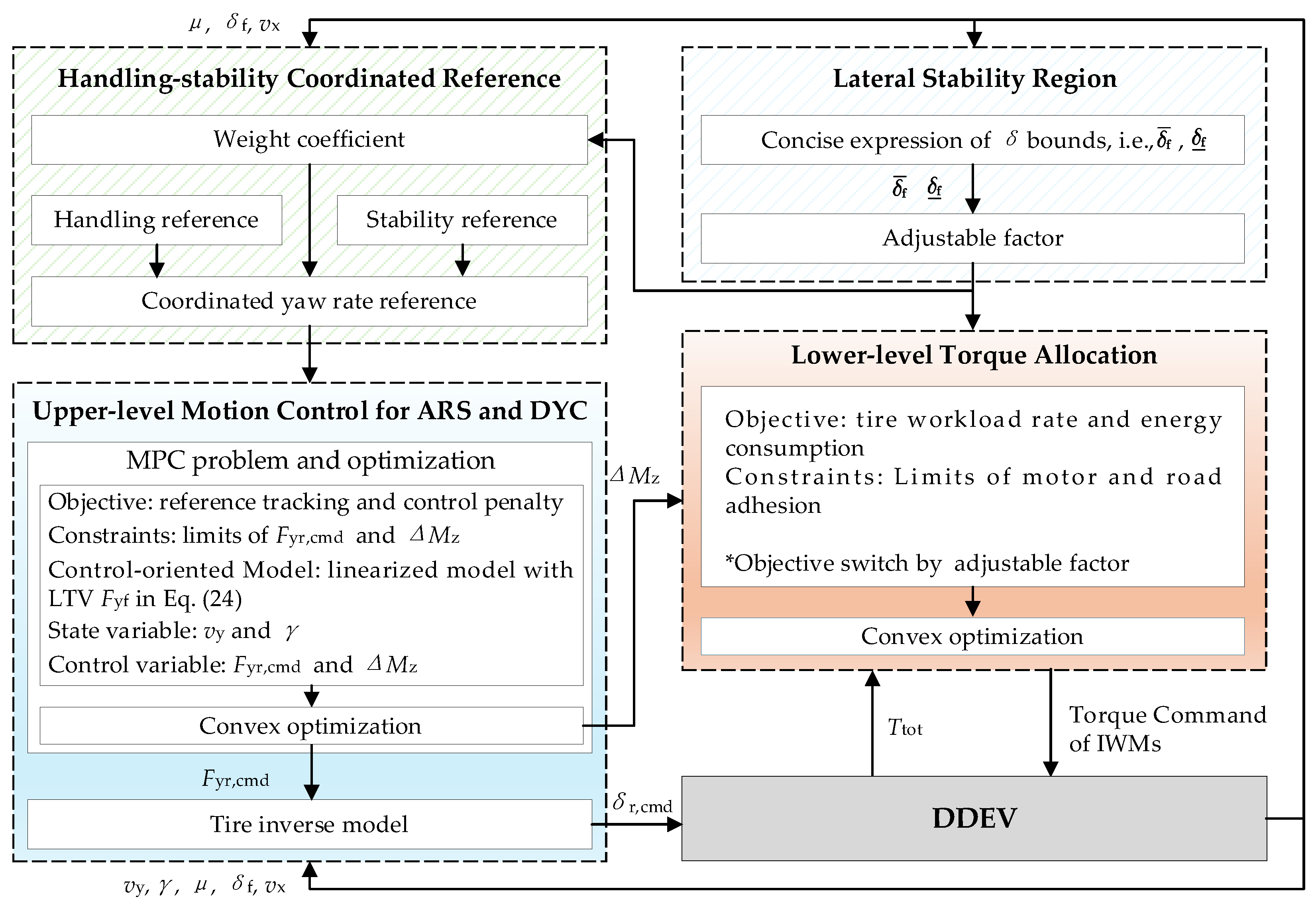
The framework of the proposed strategy is illustrated in Figure 2. Initially, the lateral stability region module assesses the vehicle’s current stability based on feedback $\mu$, ${\delta }_{\mathrm{f}}$, $v_{\mathrm{x}}$, and the established stability boundary, and the vehicle stability state is then quantitatively characterized as an adjustable factor. In the handling–stability coordinated reference module, weight coefficients are determined based on the adjustable factor, and a weighted sum of the handling reference and stability reference is calculated to formulate a combined handling and stability reference. At the upper-level motion control layer, an MPC method is developed for ARS and DYC. It targets tracking the control reference, with the rear wheel lateral force $F_{\mathrm{y}\mathrm{r},\mathrm{c}\mathrm{m}\mathrm{d}}$ and additional yaw moment $\Delta M_{\mathrm{z}}$ serving as control variables, and constraints are imposed based on the limits of the rear wheel lateral force and additional yaw moment. The optimization problem in this MPC is convex and thus can be solved rapidly. The calculated $F_{\mathrm{y}\mathrm{r},\mathrm{c}\mathrm{m}\mathrm{d}}$ is input into the tire inverse model, converted into a rear wheel steering angle command ${\delta }_{\mathrm{r},\mathrm{c}\mathrm{m}\mathrm{d}}$, and input to the vehicle to achieve ARS control. The calculated $\Delta M_{\mathrm{z}}$ is input into the lower-level TA module. In this module, as prerequisites of the total traction torque $T_{\mathrm{t}\mathrm{o}\mathrm{t}}$ and $\Delta M_{\mathrm{z}}$, the TA objectives of the tire workload rates and vehicle energy consumption are established, where the adjustable factor is used to switch between these two targets under stable and unstable conditions, achieving a synergy between energy efficiency and vehicle stability objectives. This optimization is also convex for fast solving with ease. Finally, the optimized torque commands are input to the IWMs to implement closed-loop control.

To achieve the coordination of handling, stability, and energy efficiency, the proposed strategy utilizes an upper motion controller to track the coordinated reference for handling and stability coordination. At the lower-level TA layer, considering tire workload rate optimization (for stability at the tire-ground contact interface) and motor energy efficiency objectives, a smooth transition between the two objectives is achieved through the designed adjustable factor. Ultimately, the goal of coordinated control of handling, stability, and energy efficiency for DDEV is realized. Specifically, the objective principle of this paper is to prioritize vehicle stability, followed by vehicle handling and energy efficiency. Vehicle stability is a prerequisite for ensuring driving safety, while vehicle handling enhances the driver’s driving experience. Furthermore, some studies [16] have shown that vehicle instability and sideslip can lead to extremely unreasonable motor torque output, significantly degrading vehicle energy efficiency. Additionally, research [7] has also indicated that in both lateral and longitudinal driving scenarios, a stable and well-manipulated neutral steering condition is conducive to energy savings for DDEVs. Therefore, this paper designed the control strategy with stability as the primary objective, and handling and energy efficiency as secondary objectives.

3.1. Concise Expression of Lateral Stability Region

Unlike traditional stability boundaries based on calibration, this paper conducted the design of stability region boundaries by the phase plane analysis results in [19,20]. From the $v_{\mathrm{y}}$-$\gamma$ phase plane analysis in [19,20], when a vehicle without ARS and DYC is in a critically unstable state, the upper boundaries of ${\alpha }_{\mathrm{f}}$, ${\alpha }_{\mathrm{r}}$, and $\gamma$ in the lateral motion models (7) and (8) will intersect at a saddle point on one side of the phase plane, and their lower boundaries will intersect at a saddle point on the other side. At this point, for both scenarios, three equality expressions can be obtained. Specifically, for the scenario where ${\alpha }_{\mathrm{f}}$, ${\alpha }_{\mathrm{r}}$, and $\gamma$ are all at their upper boundaries, according to (11) and (12), we can derive

$$\left\{\begin{array}{c}\overline{{\alpha }_{\mathrm{f}}}=\overline{{\delta }_{\mathrm{f}}}-arctan\left({\displaystyle \frac{\overline{v_{\mathrm{y}}}+l_{\mathrm{a}}\overline{\gamma }}{v_{\mathrm{x}}}}\right)\hfill \\ \overline{{\alpha }_{\mathrm{r}}}=arctan\left({\displaystyle \frac{l_{\mathrm{b}}\overline{\gamma }-\overline{v_{\mathrm{y}}}}{v_{\mathrm{x}}}}\right)\hfill \\ \overline{\gamma }=\mu g/v_{\mathrm{x}}\hfill \end{array}\right.$$

(13)

The three expressions above are all commonly used boundary conditions for vehicle stability. The former two are primarily to prevent the tire forces at the front and rear axles of the vehicle from entering the saturation region, which could lead to tire slip. The last condition is determined by the maximum lateral adhesion capability between the vehicle and the road surface, which is conducive to preventing vehicle sideslip.

Moreover, in (13), ${\delta }_{\mathrm{f}}$ is determined by the driver and can be regarded as an external disturbance, allowing us to discuss the stability of the vehicle in an uncontrolled scenario. Therefore, the stability boundaries discussed in this paper do not include ${\delta }_{\mathrm{r}}$ and $\Delta M_{\mathrm{z}}$. Here, $\overline{\gamma }$ adopted is based on the maximum lateral acceleration limit corresponding to adhesion [1], i.e., $\overline{\gamma }=\mu g/v_{\mathrm{x}}$, with $\overline{\gamma }=-\underset{\_}{\gamma }$. In (13), $\overline{{\alpha }_{\mathrm{f}}}$, $\overline{{\alpha }_{\mathrm{r}}}$, and $\overline{\gamma }$ are known under certain driving conditions. The first two expressions above only contain the variables $\overline{{\delta }_{\mathrm{f}}}$ and $\overline{v_{\mathrm{y}}}$, making them statically determinate. Since they both include $\overline{v_{\mathrm{y}}}$, we can replace one equation with the other to uniquely determine $\overline{\delta }$. Then, it yields:

$$\overline{{\alpha }_{\mathrm{f}}}=\overline{{\delta }_{\mathrm{f}}}-\mathrm{a}\mathrm{r}\mathrm{c}\mathrm{t}\mathrm{a}\mathrm{n}\left({\displaystyle \frac{l_{\mathrm{b}}\overline{\gamma }-v_{\mathrm{x}}\mathrm{t}\mathrm{a}\mathrm{n}\overline{{\alpha }_{\mathrm{r}}}+l_{\mathrm{a}}\overline{\gamma }}{v_{\mathrm{x}}}}\right)$$

(14)

Further, by simplifying and introducing $\overline{\gamma }=\mu g/v_{\mathrm{x}}$, we obtain:

$$\overline{{\delta }_{\mathrm{f}}}=\overline{{\alpha }_{\mathrm{f}}}+\mathrm{a}\mathrm{r}\mathrm{c}\mathrm{t}\mathrm{a}\mathrm{n}\left({\displaystyle \frac{\left(l_{\mathrm{a}}+l_{\mathrm{b}}\right)\mu g}{{v_{\mathrm{x}}}^2}}-\mathrm{t}\mathrm{a}\mathrm{n}\overline{{\alpha }_{\mathrm{r}}}\right)$$

(15)

Similarly, substituting $\underset{\_}{{\alpha }_{\mathrm{f}}}$, $\underset{\_}{{\alpha }_{\mathrm{r}}}$, and $\underset{\_}{\gamma }$ into (11) and (12), we obtain:

$$\underset{\_}{{\delta }_{\mathrm{f}}}=\underset{\_}{{\alpha }_{\mathrm{f}}}+\mathrm{a}\mathrm{r}\mathrm{c}\mathrm{t}\mathrm{a}\mathrm{n}\left({\displaystyle \frac{-\left(l_{\mathrm{a}}+l_{\mathrm{b}}\right)\mu g}{{v_{\mathrm{x}}}^2}}-\mathrm{t}\mathrm{a}\mathrm{n}\underset{\_}{{\alpha }_{\mathrm{r}}}\right)$$

(16)

The above calculation process corresponds to the critical instability scenario of the vehicle [19]. Therefore, by checking whether the current front wheel steering angle of the vehicle falls within the range of $\overline{{\delta }_{\mathrm{f}}}$ and $\underset{\_}{{\delta }_{\mathrm{f}}}$, the current driving stability of the vehicle can be assessed. Extremely, when the current front wheel steering angle is at $\overline{{\delta }_{\mathrm{f}}}$ or $\underset{\_}{{\delta }_{\mathrm{f}}}$, the vehicle is in a critical instability scenario or has a high risk of instability. Additionally, it should be noted that through (15) and (16), the stability boundaries (i.e., $\overline{{\delta }_{\mathrm{f}}}$ and $\underset{\_}{{\delta }_{\mathrm{f}}}$) can be calculated in real time, eliminating the need for offline calibration (i.e., predetermining the boundaries) and online interpolation used in most stability criterion methods. This helps reduce the workload in strategy development and the data caching burden of the controller. Based on (15) and (16), an adjustable factor ranging from 0 to 1 can be designed to quantitatively represent the current stability level:

$$\iota =\left\{\begin{array}{c}0, -0.2⩽\overline{\varpi }⩽0.2\hfill \\ 1.25\overline{\varpi }-0.25, 0.2<\overline{\varpi }⩽1\hfill \\ -1.25\overline{\varpi }-0.25, -1⩽\overline{\varpi }<-0.2\hfill \\ 1, \overline{\varpi }>1 or \overline{\varpi }<-1\hfill \end{array}\right.$$

(17)

where $\overline{\varpi }=\left(2{\delta }_{\mathrm{f}}-\left(\overline{{\delta }_{\mathrm{f}}}+\underset{\_}{{\delta }_{\mathrm{f}}}\right)\right)/\left(\overline{{\delta }_{\mathrm{f}}}-\underset{\_}{{\delta }_{\mathrm{f}}}\right)$ is a variable that normalizes ${\delta }_{\mathrm{f}}$ from $\underset{\_}{{\delta }_{\mathrm{f}}}$ to $\overline{{\delta }_{\mathrm{f}}}$ within the interval of −1 to 1. In (17), within a range of ±0.2 around the zero point on the $\overline{\varpi }$-axis, the value of $\iota$ is 0; from 0.2 to 1 on the $\overline{\varpi }$-axis, $\iota$ linearly increases from 0 to 1; from −1 to 0.2 on the $\overline{\varpi }$-axis, $\iota$ linearly decreases from 1 to 0; and for the $\overline{\varpi }$-axis, in the regions greater than 1 or less than −1, $\iota$ is set to 1. Moreover, a $\overline{\varpi }$-range of 0.4 centered at the zero point with $\iota$ of 0 is set in (17) mainly because the vehicle is considered to be stable when ${\delta }_{\mathrm{f}}$ has a small amplitude. Figure 3 shows the example illustrations about $\iota$ for varying $\overline{\varpi }$ and ${\delta }_{\mathrm{f}}$ by giving $\overline{{\delta }_{\mathrm{f}}}$ of 0.1 and $\underset{\_}{{\delta }_{\mathrm{f}}}$ of −0.05. It can be observed that as ${\delta }_{\mathrm{f}}$ changes, both $\overline{\varpi }$ and $\iota$ change as expected, and when ${\delta }_{\mathrm{f}}$ exceeds the range of $\underset{\_}{{\delta }_{\mathrm{f}}}$ to $\overline{{\delta }_{\mathrm{f}}}$, $\iota$ equals 1, indicating that the vehicle is in a critically unstable state. During the control period, real-time calculation of the adjustable factor $\iota$ can be performed using (15) to (17) based on feedback information of the front wheel steering angle, vehicle speed, and tire–road friction factor.

Remark 1. 

The phase plane state trajectory characteristics [19,20], (15), and (16), are derived from the open-loop analysis of a single-track vehicle model without ARS and DYC functionality (i.e., without inputs of${\delta }_{\mathrm{r}}$and$\Delta M_{\mathrm{z}}$). They can be adopted to assess the stability of the vehicle’s state but do not necessarily imply that a vehicle beyond these boundaries will definitely lose stability or be unable to return to a stable state. Specifically, when the vehicle’s front wheel steering angle exceeds the range encompassed by$\overline{{\delta }_{\mathrm{f}}}$and$\underset{\_}{{\delta }_{\mathrm{f}}}$, and with sufficient wheel adhesion still available, reasonable ARS and DYC control can be employed to maintain the vehicle in a stable state.

3.2. Handling-Stablity Coordinated Reference

In this paper, a yaw rate reference is established by linearly blending vehicle handling and stability references. Considering the vehicle in a steady state and using linear tire stiffness, the equilibrium points of models (7) and (8) are solved to obtain the handling reference of $\gamma$ and the stability reference of $\beta$ [21]. Additionally, to ensure lateral stability of the vehicle, the handling reference of $\gamma$ needs to be limited within $\pm \mu g/v_{\mathrm{x}}$ [1]. The resulting references are as follows:

$${\gamma }_{\mathrm{r}}=\mathrm{m}\mathrm{a}\mathrm{x}\left(\mathrm{m}\mathrm{i}\mathrm{n}\left({\displaystyle \frac{v_{\mathrm{x}}}{\left(l_{\mathrm{a}}+l_{\mathrm{b}}\right)\left(1+\sigma {v_{\mathrm{x}}}^2\right)}}{\delta }_{\mathrm{f}},\mu g/v_{\mathrm{x}}\right),-\mu g/v_{\mathrm{x}}\right)$$

(18)

$${\beta }_{\mathrm{r}}={\displaystyle \frac{l_{\mathrm{b}}-\frac{m}{l_{\mathrm{a}}+l_{\mathrm{b}}}\frac{l_{\mathrm{a}}}{C_{\mathrm{r}}}{v_{\mathrm{x}}}^2}{\left(l_{\mathrm{a}}+l_{\mathrm{b}}\right)\left(1+\sigma {v_{\mathrm{x}}}^2\right)}}{\delta }_{\mathrm{f}}$$

(19)

where ${\gamma }_{\mathrm{r}}$ is the handling reference, and ${\beta }_{\mathrm{r}}$ is the stability reference. $\sigma =m\left(l_{\mathrm{b}}{C}_{\mathrm{r}}-l_{\mathrm{a}}{C}_{\mathrm{f}}\right)/\left[{\left(l_{\mathrm{a}}+l_{\mathrm{b}}\right)}^2{C}_{\mathrm{f}}{C}_{\mathrm{r}}\right]$ is the stability coefficient, describing the steering characteristics of the vehicle. $C_{\mathrm{f}}$ and $C_{\mathrm{r}}$ are the linear tire stiffnesses of the front and rear wheels, respectively. It is noteworthy that the control reference here represents the expected vehicle handling and stability performance, i.e., the driver’s desired vehicle behavior, so the driver’s front wheel steering angle input ${\delta }_{\mathrm{f}}$ is applied for calculation. Herein, the coordinated control reference for handling and stability is defined as an expression related to $\gamma$, which is the weighted sum of (18) and (19), i.e., ${\gamma }_{\mathrm{h}-\mathrm{s}}={\gamma }_{\mathrm{r}}+W{\beta }_{\mathrm{r}}$. A real-time variable weight $W$ can be further developed in combination with (17) to enhance the coordinated effect of vehicle handling and stability. In this paper, $W$ is set as

$$W=\left\{\begin{array}{c}{\kappa }_{\mathrm{h}}, \iota =0\\ \left(-{\kappa }_{\mathrm{h}}+{\kappa }_{\mathrm{l}}\right)\iota +{\kappa }_{\mathrm{h}}, 0<\iota <1\\ {\kappa }_{\mathrm{l}}, \iota =1\end{array}\right.$$

(20)

where ${\kappa }_{\mathrm{l}}$ and ${\kappa }_{\mathrm{h}}$ are two coefficients. According to the zero dynamics analysis of the vehicle motion in [22], the range of weight coefficient values that can achieve the differentiation of zeroing the sideslip angle and yaw rate is $-v_{\mathrm{x}}/l_{\mathrm{r}}⩽W<-0.5$; specifically, as $W$ increases and approaches −0.5, ${\gamma }_{\mathrm{h}-\mathrm{s}}$ tends towards the handling target, while as $W$ decreases, ${\gamma }_{\mathrm{h}-\mathrm{s}}$ will approach the stability target. Therefore, to maximize the handling target as much as possible when the vehicle is driving stably ($\iota$ closes to 0), it is necessary to minimize the influence of ${\beta }_{\mathrm{r}}$ in ${\gamma }_{\mathrm{h}-\mathrm{s}}={\gamma }_{\mathrm{r}}+W{\beta }_{\mathrm{r}}$. Thus, this paper chooses ${\kappa }_{\mathrm{h}}$ as 0 in (20). When the vehicle is critically unstable, it is necessary to keep $W$ within $\left[-v_{\mathrm{x}}/l_{\mathrm{r}},-0.5\right]$ to ensure that the vehicle can effectively converge to the reference and maintain stability. Hence, ${\kappa }_{\mathrm{l}}$ is selected as −1.5 herein.

3.3. High Layer Control: Motion Control

In this paper, the upper-level motion control layer employs the MPC method for ARS and DYC. For ARS, unlike traditional studies that use the rear wheel steering angle command ${\delta }_{\mathrm{r},\mathrm{c}\mathrm{m}\mathrm{d}}$ for control, this paper adopts the desired front wheel lateral force $F_{\mathrm{y}\mathrm{r},\mathrm{c}\mathrm{m}\mathrm{d}}$ as the control variable to simplify the model complexity. $F_{\mathrm{y}\mathrm{r},\mathrm{c}\mathrm{m}\mathrm{d}}$ is then converted into ${\delta }_{\mathrm{r},\mathrm{c}\mathrm{m}\mathrm{d}}$ and input into the vehicle for AFS. By this manner, the nonlinear terms in the Magic Formula tire model (9) and the rear wheel sideslip angle Equation (11) can be avoided, enabling a linear relationship between the state derivatives and the control in MPC optimization. This simplifies the control complexity and contributes to improving computational efficiency in MPC. To carry out the above transformation from $F_{\mathrm{y}\mathrm{r},\mathrm{c}\mathrm{m}\mathrm{d}}$ to ${\delta }_{\mathrm{r},\mathrm{c}\mathrm{m}\mathrm{d}}$, a tire inverse model should be established first, as described below.

3.3.1. Tire Inverse Model

Based on the tire model (9), the rear wheel sideslip angle can be expressed as

$${\alpha }_{\mathrm{r}}={\mathsf{\Psi }}_{\mathrm{y}\_\mathrm{i}\mathrm{n}\mathrm{v}}\left(F_{\mathrm{y}\mathrm{r},\mathrm{c}\mathrm{m}\mathrm{d}},\mu ,F_{\mathrm{z}\mathrm{r}}\right)$$

(21)

where ${\mathsf{\Psi }}_{\mathrm{y}\_\mathrm{i}\mathrm{n}\mathrm{v}}\left(\right)$ denotes the inverse function of (9). This paper assumes that the controller can effectively ensure vehicle stability, so the actual tire lateral force can be limited within the unsaturated region, i.e., $\underset{\_}{{\alpha }_{\mathrm{r}}}⩽{\alpha }_{\mathrm{r}}⩽\overline{{\alpha }_{\mathrm{r}}}$. Hence, for a given group of $\mu$ and $F_{\mathrm{z}\mathrm{r}}$, a unique $F_{\mathrm{y}\mathrm{r},\mathrm{c}\mathrm{m}\mathrm{d}}$ within a peak lateral force range corresponds to a unique ${\alpha }_{\mathrm{r}}$, establishing the aforementioned mapping relationship.

Further, combining (12), we obtain:

$${\delta }_{\mathrm{r},\mathrm{c}\mathrm{m}\mathrm{d}}={\alpha }_{\mathrm{r}}+\mathrm{a}\mathrm{r}\mathrm{c}\mathrm{t}\mathrm{a}\mathrm{n}\left({\displaystyle \frac{v_{\mathrm{y}}-l_{\mathrm{b}}\gamma }{v_{\mathrm{x}}}}\right)$$

(22)

Integrating (21) and (22), the rear wheel steering angle input can be derived as

$${\delta }_{\mathrm{r},\mathrm{c}\mathrm{m}\mathrm{d}}={\mathsf{\Psi }}_{\mathrm{y}\_\mathrm{i}\mathrm{n}\mathrm{v}}\left(F_{\mathrm{y}\mathrm{r},\mathrm{c}\mathrm{m}\mathrm{d}},\mu ,F_{\mathrm{z}\mathrm{r}}\right)+\mathrm{a}\mathrm{r}\mathrm{c}\mathrm{t}\mathrm{a}\mathrm{n}\left({\displaystyle \frac{v_{\mathrm{y}}-l_{\mathrm{b}}\gamma }{v_{\mathrm{x}}}}\right)$$

(23)

In the above equation, the relationship in ${\mathsf{\Psi }}_{\mathrm{y}\_\mathrm{i}\mathrm{n}\mathrm{v}}\left(\right)$ can be obtained by iterating through all possible values of $F_{\mathrm{y}\mathrm{r},\mathrm{c}\mathrm{m}\mathrm{d}}$, $\mu$, and $F_{\mathrm{z}\mathrm{r}}$, and calculating the corresponding ${\alpha }_{\mathrm{r}}$, which is then recorded and saved as an interpolation table for online application. In this paper, the ranges for $F_{\mathrm{y}\mathrm{r},\mathrm{c}\mathrm{m}\mathrm{d}}$, $\mu$, and $F_{\mathrm{z}\mathrm{r}}$, are set to [$-\mu F_{\mathrm{z}\mathrm{r}}:10:\mu F_{\mathrm{z}\mathrm{r}}$], [0.2:0.1:1], and [0:500:8000], respectively. The established look-up table of ${\mathsf{\Psi }}_{\mathrm{y}\_\mathrm{i}\mathrm{n}\mathrm{v}}\left(\right)$ for $F_{\mathrm{z}\mathrm{r}}$ of 4000 N and 7000 N is shown in Figure 4. One can find that, when $\mu$ is constant, ${\alpha }_{\mathrm{r}}$ increases monotonically with an increasing rate as $F_{\mathrm{y}\mathrm{r},\mathrm{c}\mathrm{m}\mathrm{d}}$ increases, remaining constant after reaching the peak tire force corresponding to the maximum rear wheel sideslip angle. As $\mu$ increases, the maximum ${\alpha }_{\mathrm{r}}$ also increases, consistent with the characteristics of the Magic Formula tire model.

3.3.2. Predictive Controller for ARS and DYC

The MPC approach [23] for ARS and DYC is introduced in this section. To simplify calculations, the front wheel lateral force is linearized based on the Taylor expansion point ${\alpha }_{\mathrm{f}0}$, where ${\alpha }_{\mathrm{f}0}$ is the sideslip angle of front tires at the current time. Using the concept of LTV [24], the front wheel lateral force can be expressed as $F_{\mathrm{y}\mathrm{f},\mathrm{l}\mathrm{i}\mathrm{n}\mathrm{e}\mathrm{a}\mathrm{r}}=F_{\mathrm{y}\mathrm{f}0}+C_{\mathrm{f},\mathrm{l}\mathrm{i}\mathrm{n}\mathrm{e}\mathrm{a}\mathrm{r}}\left({\alpha }_{\mathrm{f}}-{\alpha }_{\mathrm{f}0}\right)$, where $F_{\mathrm{y}\mathrm{f}0}$ is the front wheel lateral force of ${\alpha }_{\mathrm{f}0}$, and $C_{\mathrm{f},\mathrm{l}\mathrm{i}\mathrm{n}\mathrm{e}\mathrm{a}\mathrm{r}}$ is the local cornering stiffness at ${\alpha }_{\mathrm{f}0}$. Based on $F_{\mathrm{y}\mathrm{f},\mathrm{l}\mathrm{i}\mathrm{n}\mathrm{e}\mathrm{a}\mathrm{r}}$, (7) and (8), the following state equations can be furnished:

$$\left\{\begin{array}{c}\dot{x}\left(t\right)=Ax\left(t\right)+Bu\left(t\right)+d_t\hfill \\ y\left(t\right)=Dx\left(t\right)\hfill \end{array}\right.$$

(24)

where $x={\left[v_{\mathrm{y}},\gamma \right]}^{\mathrm{T}}$, $u={\left[F_{\mathrm{y}\mathrm{r},\mathrm{c}\mathrm{m}\mathrm{d}},\Delta M_{\mathrm{z}}\right]}^{\mathrm{T}}$, $D=I_{2\times 2}$,

$$A=\left[\begin{array}{cc}-{\displaystyle \frac{C_{\mathrm{f},\mathrm{l}\mathrm{i}\mathrm{n}\mathrm{e}\mathrm{a}\mathrm{r}}}{m{v}_{\mathrm{x}}}}& -{\displaystyle \frac{C_{\mathrm{f},\mathrm{l}\mathrm{i}\mathrm{n}\mathrm{e}\mathrm{a}\mathrm{r}}{l}_{\mathrm{a}}}{m{v}_{\mathrm{x}}}}-v_{\mathrm{x}}\\ -{\displaystyle \frac{C_{\mathrm{f},\mathrm{l}\mathrm{i}\mathrm{n}\mathrm{e}\mathrm{a}\mathrm{r}}{l}_{\mathrm{a}}}{I_{\mathrm{z}}{v}_{\mathrm{x}}}}& -{\displaystyle \frac{C_{\mathrm{f},\mathrm{l}\mathrm{i}\mathrm{n}\mathrm{e}\mathrm{a}\mathrm{r}}{l_{\mathrm{a}}}^2}{I_{\mathrm{z}}{v}_{\mathrm{x}}}}\end{array}\right],B=\left[\begin{array}{cc}{\displaystyle \frac{1}{m}}& 0\\ -{\displaystyle \frac{l_{\mathrm{b}}}{I_{\mathrm{z}}}}& {\displaystyle \frac{1}{I_{\mathrm{z}}}}\end{array}\right],d_t=\left[\begin{array}{c}{\displaystyle \frac{1}{m}}{F}_{\mathrm{y}\mathrm{f}0}+{\displaystyle \frac{1}{m}}{C}_{\mathrm{f},\mathrm{l}\mathrm{i}\mathrm{n}\mathrm{e}\mathrm{a}\mathrm{r}}{\delta }_{\mathrm{f}}-{\displaystyle \frac{1}{m}}{C}_{\mathrm{f},\mathrm{l}\mathrm{i}\mathrm{n}\mathrm{e}\mathrm{a}\mathrm{r}}{\alpha }_{\mathrm{f}0}\\ {\displaystyle \frac{l_{\mathrm{a}}}{I_{\mathrm{z}}}}{F}_{\mathrm{y}\mathrm{f}0}+{\displaystyle \frac{l_{\mathrm{a}}}{I_{\mathrm{z}}}}{C}_{\mathrm{f},\mathrm{l}\mathrm{i}\mathrm{n}\mathrm{e}\mathrm{a}\mathrm{r}}{\delta }_{\mathrm{f}}-{\displaystyle \frac{l_{\mathrm{a}}}{I_{\mathrm{z}}}}{C}_{\mathrm{f},\mathrm{l}\mathrm{i}\mathrm{n}\mathrm{e}\mathrm{a}\mathrm{r}}{\alpha }_{\mathrm{f}0}\end{array}\right].$$

Using zero-order hold (ZOH) for model discretization with respect to the sampling step $t_{\mathrm{s}}$, there is

$$\left\{\begin{array}{c}x\left(k+1\right)=A_{\mathrm{d}}x\left(k\right)+B_{\mathrm{d}}u\left(k\right)+d_t\hfill \\ y\left(k\right)=Dx\left(k\right)\hfill \end{array}\right.$$

(25)

where $A_{\mathrm{d}}=e^{A{t}_{\mathrm{s}}}$, $B_{\mathrm{d}}={\int }_0^{t_{\mathrm{s}}}{e}^{A\tau }d\tau \cdot B$, and $d_t={\int }_0^{t_{\mathrm{s}}}{e}^{A\tau }d\tau \cdot d_t$. For desired handling and stability performance, the following control objective is set up,

$$J_{\mathrm{M}\mathrm{P}\mathrm{C}}={\sum }_{i=0}^{N_{\mathrm{p}}-1}Q{\left(\gamma \left(k+i|k\right)-{\gamma }_{\mathrm{h}-\mathrm{s}}\left(k+i|k\right)\right)}^2+{\sum }_{i=0}^{N_{\mathrm{p}}-1}R{\left(u\left(k+i|k\right)-u\left(k\right)\right)}^2$$

(26)

where $N_{\mathrm{p}}$ is the predictive horizon length. $Q$ and $R$ are weight matrices, respectively. Additionally, the control constraints are considered:

$$\underset{\_}{F_{\mathrm{y}\mathrm{r},\mathrm{c}\mathrm{m}\mathrm{d}}}⩽F_{\mathrm{y}\mathrm{r},\mathrm{c}\mathrm{m}\mathrm{d}}⩽\overline{F_{\mathrm{y}\mathrm{r},\mathrm{c}\mathrm{m}\mathrm{d}}}$$

(27)

$$\underset{\_}{\Delta M_{\mathrm{z}}}⩽\Delta M_{\mathrm{z}}⩽\overline{\Delta M_{\mathrm{z}}}$$

(28)

where the limits in (27) are equal to the peak lateral forces at $\overline{{\alpha }_{\mathrm{r}}}$ and $\underset{\_}{{\alpha }_{\mathrm{r}}}$, respectively. For the above optimization problem, it should be noted: firstly, since the designed handling and stability reference already considers the vehicle stability requirements, no state constraints related to vehicle stability are included here; and secondly, based on (24) and (26), the objective expression is linear with respect to the control variable $u$ (the optimized variable), and the constraints (27) and (28) are affine functions, hence this is a convex optimization problem that can be solved quickly. In this paper, the widely used convex optimization method, interior point method (IPM), is selected for real-time optimization of the MPC problem.

In each control period, the MPC optimization is performed to output the desired $F_{\mathrm{y}\mathrm{r},\mathrm{c}\mathrm{m}\mathrm{d}}$ and $\Delta M_z$. $F_{\mathrm{y}\mathrm{r},\mathrm{c}\mathrm{m}\mathrm{d}}$ is then converted into a rear wheel steering angle command ${\delta }_{\mathrm{r},\mathrm{c}\mathrm{m}\mathrm{d}}$ via the tire inverse model (23) and input to the vehicle, while $\Delta M_z$ is transmitted to the lower level as a generalized control force for TA optimization.

Remark 2. 

Generally, when the vehicle is in a steady driving state (with unsaturated tire forces), the trajectories of the vehicle’s motion states$\gamma$and$\beta$are close to the control references (18) and (19), respectively, signifying that the tracking deviation of$\gamma$in the aforementioned MPC problem is small and the control variable$u$is close to 0 [18]. That is, when the vehicle is driving stably, whether the upper-level motion control optimizes motor efficiency has a minor impact on the overall vehicle economy [16]. Therefore, in this paper, the upper level does not introduce motor efficiency optimization terms with strongly nonlinear expressions to simplify the control problem. Instead, motor efficiency optimization is considered at the TA layer.

Remark 3. 

For MPC, as the prediction horizon increases, the accuracy of the linear state update equation may become slightly inadequate, potentially affecting control effects. Conversely, using a nonlinear state equation (such as if this paper considered a nonlinear tire model) would enhance the accuracy of the future state trajectory within the prediction horizon but at a significant computational cost. Therefore, this paper adopts a compromise approach by selecting the rear-axle tire force as the control input and representing the front-wheel lateral force in an LTV manner to establish a linear control-oriented model (24). The rear-axle tire force control input is then converted into a rear-wheel steering angle command using a tire inverse model (23). This approach can restore the nonlinear relationship of the rear-axle tire lateral force as much as possible. Meanwhile, the front-wheel lateral force is approximated using Taylor series expansion at the current state point, which helps reduce model errors and improve control performance. Given this, an MPC optimization problem is formulated in (26) to (28), and its convex optimization properties are demonstrated. Consequently, the proposed MPC controller can achieve high computational efficiency.

3.4. Lower Layer Control: Torque Allocation

For the desirable vehicle motion, the TA layer should satisfy the generalized control force requirement, namely,

$$\vartheta =B_{\vartheta }\nu$$

(29)

where $\vartheta ={\left[T_{\mathrm{t}\mathrm{o}\mathrm{t}},\Delta M_{\mathrm{z}}\right]}^{\mathrm{T}}$ is the generalized control force vector, and $\nu ={\left[T_{\mathrm{f}\mathrm{l}},T_{\mathrm{f}\mathrm{r}},T_{\mathrm{r}\mathrm{l}},T_{\mathrm{r}\mathrm{r}}\right]}^{\mathrm{T}}$ is the vector composed of torque commands for each IWM. $B_{\vartheta }$ is written as

$$B_{\vartheta }={\displaystyle \frac{1}{r_{\mathrm{w}}}}\left[\begin{array}{cccc}1& 1& 1& 1\\ -{\displaystyle \frac{d_{\mathrm{t}}}{2}}& {\displaystyle \frac{d_{\mathrm{t}}}{2}}& -{\displaystyle \frac{d_{\mathrm{t}}}{2}}& {\displaystyle \frac{d_{\mathrm{t}}}{2}}\end{array}\right]$$

To maximize tire stability margin, the objective function for minimizing tire workload rate [20] is given by

$$J_{\mathrm{w}\mathrm{o}\mathrm{r}\mathrm{k}\mathrm{l}\mathrm{o}\mathrm{a}\mathrm{d}}={\sum }_{\ast =\mathrm{f}\mathrm{l},\mathrm{f}\mathrm{r},\mathrm{r}\mathrm{l},\mathrm{r}\mathrm{r}}{\displaystyle \frac{{T_{\ast }}^2}{{r_{\mathrm{w}}}^2{\mu }^2{F_{\mathrm{z}\ast }}^2}}$$

(30)

Besides, motor efficiency optimization needs to be considered at the lower level, with the goal of minimizing the sum of internal powers of each motor, expressed as

$$J_{\mathrm{e}\mathrm{n}\mathrm{e}\mathrm{r}\mathrm{g}\mathrm{y}}={\sum }_{\ast =\mathrm{f}\mathrm{l},\mathrm{f}\mathrm{r},\mathrm{r}\mathrm{l},\mathrm{r}\mathrm{r}}{P}_{\mathrm{m}\mathrm{i}\ast }$$

(31)

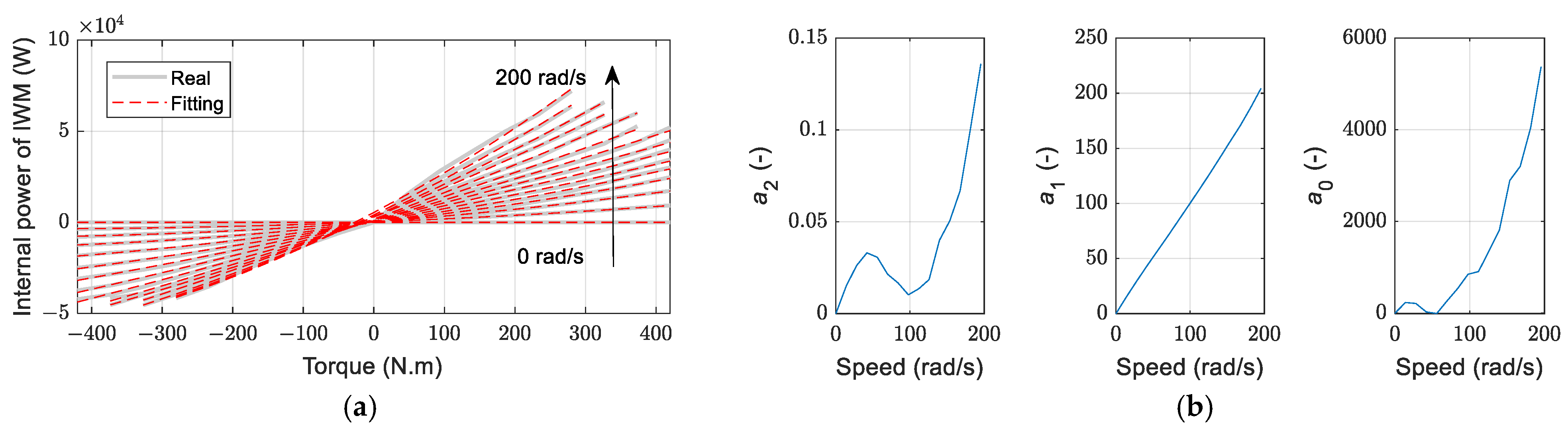
Since the motor efficiency curve at a certain speed generally exhibits an approximately concave shape (see Figure 1), according to (2), a quadratic expression can be used to fit $P_{\mathrm{m}\mathrm{i}\ast }$ for model complexity simplification, resulting in

$$P_{\mathrm{m}\mathrm{i}\ast }=a_2\left(w_{\ast }\right)\times {T_{\ast }}^2+a_1\left(w_{\ast }\right)\times T_{\ast }+a_0\left(w_{\ast }\right)$$

(32)

where $a_2\left(w_{\ast }\right)$, $a_1\left(w_{\ast }\right)$, and $a_0\left(w_{\ast }\right)$ are fitting coefficients at a speed $w_{\ast }$. The fitting results and fitting coefficients of (32) are depicted in Figure 5. From Figure 5a, Equation (32) can fit the model relationship between $T_{\ast }$ and $P_{\mathrm{m}\mathrm{i}\ast }$ with high accuracy, making it suitable for controller design. In each control period of the TA, we have $w_{\ast }\approx v_{\mathrm{x}}/r_{\mathrm{w}}$, which can be calculated from the feedback $v_{\mathrm{x}}$. In other words, before each optimization of TA, $w_{\ast }$ is known and constant, so the fitting coefficients can be calculated using the relationship in Figure 5b for energy consumption optimization.

To coordinate the targets of vehicle stability and energy efficiency, the adjustable factor $\iota$ that represents the current vehicle stability status is employed to establish the following weighted sum form of the TA optimization objective:

$$J_{\mathrm{T}\mathrm{A}}=\iota J_{\mathrm{w}\mathrm{o}\mathrm{r}\mathrm{k}\mathrm{l}\mathrm{o}\mathrm{a}\mathrm{d}}+\rho \left(1-\iota \right)J_{\mathrm{e}\mathrm{n}\mathrm{e}\mathrm{r}\mathrm{g}\mathrm{y}}$$

(33)

where $\rho$ is a coefficient less than 1 to balance the magnitude differences between $J_{\mathrm{w}\mathrm{o}\mathrm{r}\mathrm{k}\mathrm{l}\mathrm{o}\mathrm{a}\mathrm{d}}$ and $J_{\mathrm{e}\mathrm{n}\mathrm{e}\mathrm{r}\mathrm{g}\mathrm{y}}$. Combining the analysis in Section 3.1, Equation (33) enables switching between the stability and energy efficiency control objectives. 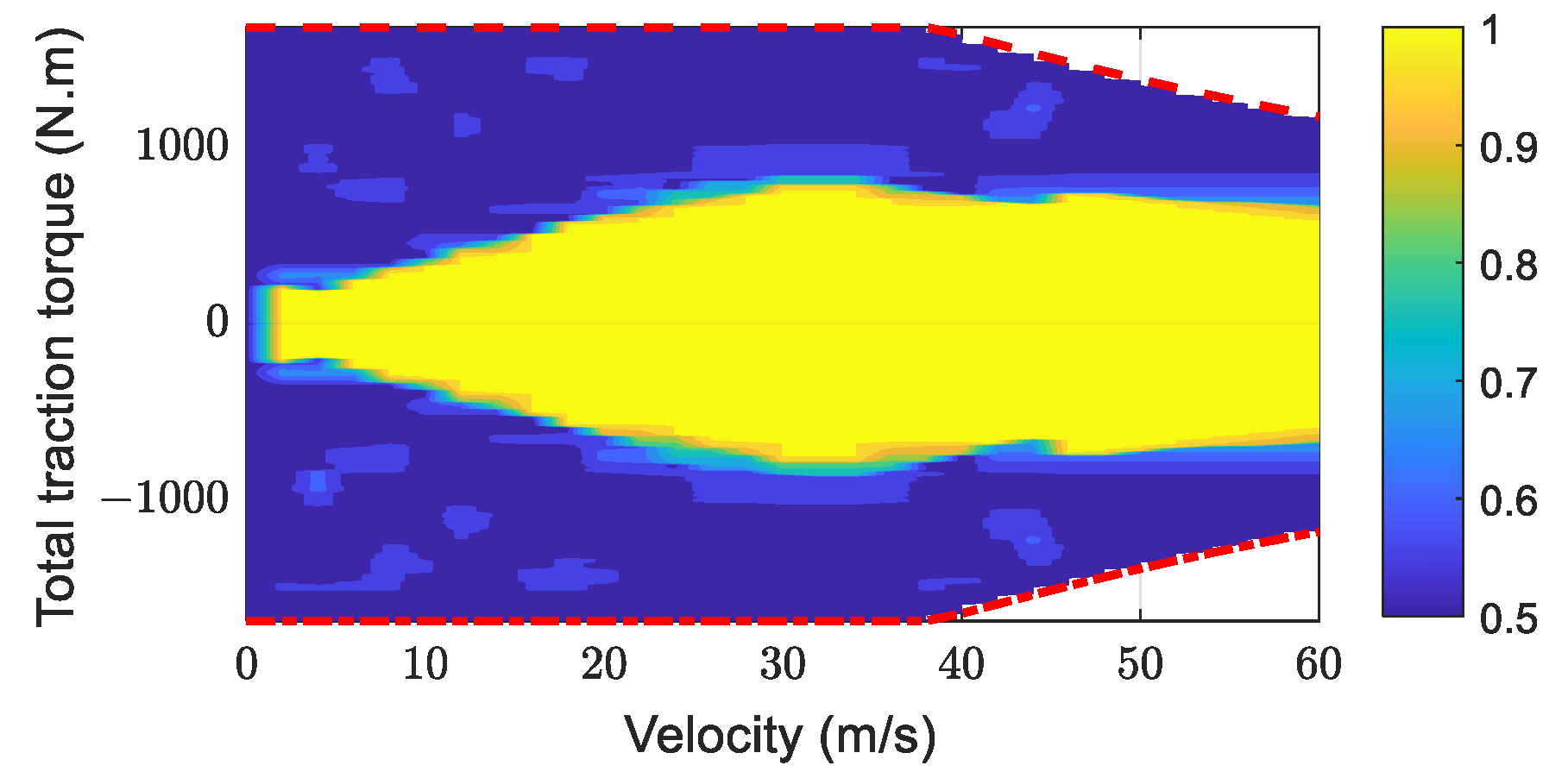Specifically, when the vehicle is critically unstable, $\iota$ is 1, and only the term $J_{\mathrm{w}\mathrm{o}\mathrm{r}\mathrm{k}\mathrm{l}\mathrm{o}\mathrm{a}\mathrm{d}}$ remains in (33) to maximize vehicle stability as much as possible. The constraints for the TA problem are arranged as

$$\vartheta =B_{\vartheta }\nu$$

(34)

$$\mathrm{m}\mathrm{a}\mathrm{x}\left(\underset{\_}{T_{\ast }},-r_{\mathrm{w}}\sqrt{{\left(\mu F_{\mathrm{z}\ast }\right)}^2-{F_{\mathrm{y}\ast }}^2}\right)⩽T_{\ast }⩽\mathrm{m}\mathrm{i}\mathrm{n}\left(\overline{T_{\ast }},r_{\mathrm{w}}\sqrt{{\left(\mu F_{\mathrm{z}\ast }\right)}^2-{F_{\mathrm{y}\ast }}^2}\right),\ast =\mathrm{f}\mathrm{l},\mathrm{f}\mathrm{r},\mathrm{r}\mathrm{l},\mathrm{r}\mathrm{r}$$

(35)

In (35), the first term inside the brackets represents the physical limit of motor torque, and the second term represents the torque constraints for each IWM calculated inversely from the tire adhesion ellipse (i.e., allowable adhesion limit) expression ${F_{\mathrm{x}\ast }}^2+{F_{\mathrm{y}\ast }}^2⩽{\mu }^2{F_{\mathrm{z}\ast }}^2$ [18] to prevent tire slip.

For the TA problem above, all variables except the optimized variables (i.e., torque commands) can be determined before optimization. The optimization objective is a linear combination of $J_{\mathrm{w}\mathrm{o}\mathrm{r}\mathrm{k}\mathrm{l}\mathrm{o}\mathrm{a}\mathrm{d}}$ and $J_{\mathrm{e}\mathrm{n}\mathrm{e}\mathrm{r}\mathrm{g}\mathrm{y}}$. $J_{\mathrm{w}\mathrm{o}\mathrm{r}\mathrm{k}\mathrm{l}\mathrm{o}\mathrm{a}\mathrm{d}}$ is a convex function, and since $a_2\left(w_{\ast }\right)$ is greater than 0 across the entire range of $w_{\ast }$, $J_{\mathrm{e}\mathrm{n}\mathrm{e}\mathrm{r}\mathrm{g}\mathrm{y}}$ is also a convex function. Therefore, the optimization objective (33) in TA is convex. As for the constraints, both (34) and (35) are affine functions. Thus, the formulated TA problem herein is a convex optimization problem that can be solved quickly using the IPM.

4. Simulation Validations and Discussions

In this paper, the proposed strategy was validated through a co-simulation platform of MATLAB/Simulink and CarSim [25], and a laptop computer with a Core(TM) i9 processor at 2.2 GHz and 32 GB of RAM was delegated. The main parameters of the DDEV and control strategy are listed in

Table 1. Parameters for DDEV and control strategy.

Item	Value	Unit
Vehicle mass	1412	kg
Distance from CoG to front axle	1.015	m
Distance from CoG to rear axle	1.895	m
Wheel track	1.675	m
Wheel radius	0.308	m
Yaw inertia	1536.7	kg·m2
Predictive horizon length	10	/
Control step	0.02	s

. It should be noted that for MPC, a longer prediction horizon can provide more dynamic information about the model, allowing the MPC to “look ahead” further and potentially improve control performance to some extent. However, this also increases the computational burden. Conversely, a shorter prediction horizon results in less information being obtained about future state trajectories, which may limit the optimization effect, but it enhances computational efficiency. Referring to research on MPC-based vehicle control [1], this paper selected a prediction horizon of 10, as this parameter was sufficient for the controller to adjust the vehicle’s state under high-speed extreme conditions.

To fully validate the proposed method, comparisons were made with no control (named “nCTR”), EETA, and LQR-DTA strategies. Specifically, the nCTR strategy adopts an equal TA method, where the total traction torque is evenly distributed to each IWM. The EETA method, derived from [16], involves offline calibration of the optimal energy-efficiency front-to-rear axle TA ratio for different $T_{\mathrm{t}\mathrm{o}\mathrm{t}}$ and $v_{\mathrm{x}}$ values, followed by online interpolation and equal distribution of the calculated front/rear axle torque to both sides’ IWMs. The mapping relations of front-to-rear axle TA ratios in this paper is shown in Figure 6. Compared with the first two methods, LQR-DTA introduces ARS and DYC functionalities. Building upon the strategy of DYC and TA [15] that considers both energy efficiency and handling stability, we additionally incorporated the ARS function into the LQR controller. That is, the upper-level control in the LQR-DTA herein uses ${\delta }_{\mathrm{r},\mathrm{c}\mathrm{m}\mathrm{d}}$ and $\Delta M_{\mathrm{z}}$ as control commands to achieve simultaneous ARS and DYC. At the lower-level layer, a DTA method is employed, which primarily involves calculating the total torque for the left and right sides of the DDEV based on $T_{\mathrm{t}\mathrm{o}\mathrm{t}}$ and $\Delta M_{\mathrm{z}}$, and then distributing the torque of the front and rear IWM on one side according to the vehicle’s static load distribution. This strategy achieves superior handling stability and economy when only applying DYC at the upper level [15]. Therefore, we modified the LQR-DTA method with ARS for comprehensive comparison.

The double lane change (DLC) drive cycle [26] was employed for testing, with two driving scenarios set up as (1) Case 1: velocity of 100 km/h and tire-road friction factor of 0.8; (2) Case 2: velocity of 90 km/h, and tire-road friction factor of 0.4. The reference path adopted herein is illustrated in Figure 7. It is from the software CarSim, and with four aggressive turning operations. Under this driving cycle, tests were conducted at speeds of 90 km/h and 100 km/h on both high and low adhesion road surfaces in this paper, which meet the requirements for extreme driving scenarios involving high speeds or/and low adhesion road surfaces, allowing for a comprehensive and effective validation of the proposed strategy.

4.1. Coordinated Control Reference, Adjustable Factor, and Weight

Figure 8 shows the results of yaw rate reference, adjustable factor, and weight coefficient by the proposed strategy under Case 1 and Case 2 drive cycles. As shown in Figure 8b,c, during cornering, as the front wheel angle increases to the stability limits defined by (15) and (16), the adjustable factor gradually increases from 0 to 1. Specifically, the adjustable factor reaches its maximum value, closest to 1, at the four steering time points in DLC, indicating that the vehicle is prone to instability at these moments. As the adjustable factor increases, the weight coefficient decreases from 0 to −1.5 to minimize the amplitude of the yaw rate reference (see the red line in the yaw rate plot) and ensure stable vehicle operation. With this operating mechanism, the proposed yaw rate reference is almost equal to the handling reference when the vehicle is stable, and reduces the yaw rate reference amplitude for drive stability when the vehicle is near the stability limit. This facilitates the coordination of vehicle handling and stability, as illustrated in Figure 8a,b. In summary, the proposed control reference can effectively achieve the switch between handling and stability references in time, consistent with expectations.

4.2. Performance Under Case 1 and Case 2

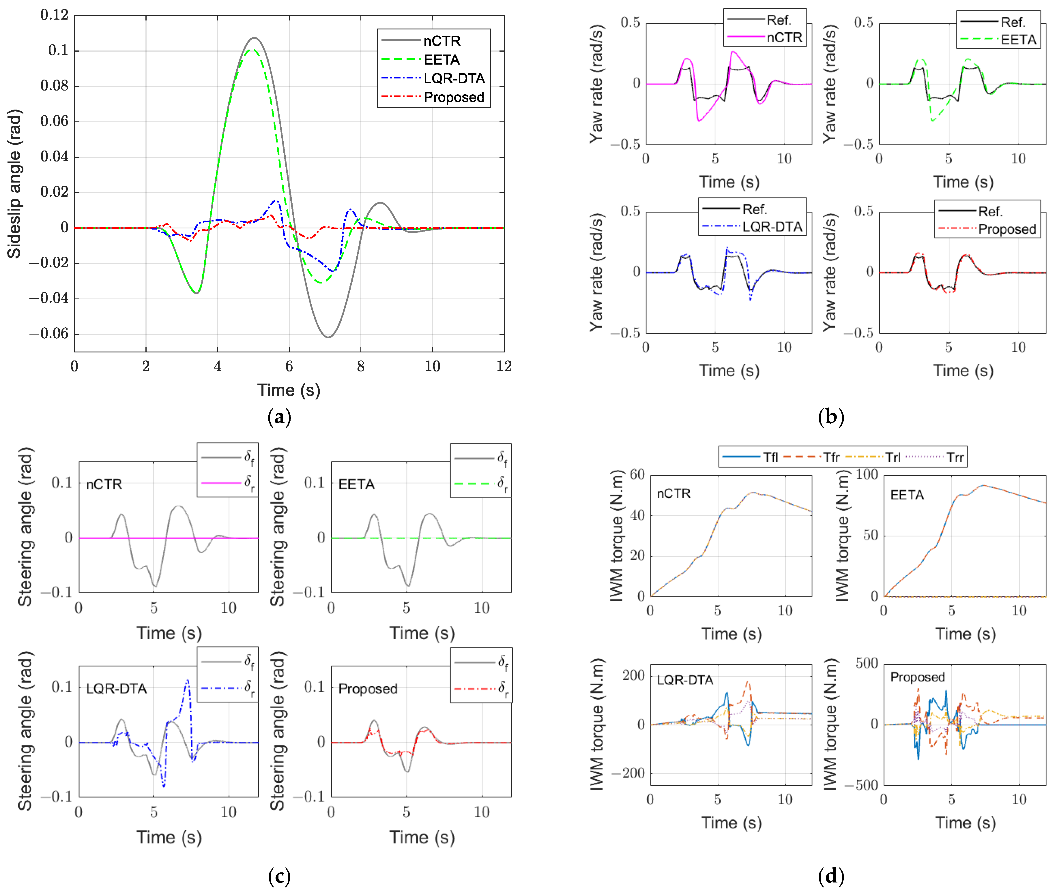
Figure 9 illustrates the performance of nCTR, EETA, LQR-DTA, and the proposed strategy under Case 1 conditions. As shown in Figure 9a, compared with the nCTR and EETA without ARS and DYC functionalities, LQR-DTA and the proposed strategy exhibited smaller sideslip angles, indicating superior stability. Figure 9b demonstrates that the proposed strategy, leveraging a tire inverse model for ARS control, effectively considers rear wheel nonlinearity in MPC, enhancing control performance and achieving higher tracking accuracy than other strategies. As shown in Figure 9c, the driver’s front wheel steering angle input and rear wheel steering command amplitudes for the LQR-DTA method are larger and yield more pronounced jitter than those of the proposed strategy. This is primarily due to LQR-DTA’s use of a linear tire model for both front and rear axle lateral forces, which, during steering under DLC conditions, cannot adapt tire force nonlinearity, making it difficult to immediately eliminate tracking errors caused by model discrepancies. In contrast, the proposed strategy incorporates a tire inverse model and linearizes the front wheel lateral force using the LTV approach, minimizing errors arising from front and rear wheel lateral force models. During straight-line driving in Case 1, the vehicle operated in a steady state, with the optimal torque distribution for instantaneous energy consumption being front-wheel drive, as shown in Figure 6. Consequently, in Figure 9d, the EETA strategy utilizes only the front axle IWMs for propulsion. The IWMs’ torque of the proposed strategy also transitioned to front-wheel drive after around 7 s, demonstrating its adaptability to optimal energy efficiency demands during stable straight-line driving.

Figure 10 presents the performance of nCTR, EETA, LQR-DTA, and the proposed strategy under Case 2 conditions. Compared with the results for Case 1 in Figure 9, the results under Case 2 on a low-adhesion surface were significantly more aggressive. Under this drive cycle, the proposed strategy still implemented the smallest sideslip angle amplitude, indicating the best stability. Besides, compared to other strategies, the smallest yaw rate reference tracking error and a smoother actual yaw rate are conducted by the proposed strategy. Figure 10c yields that due to its use of a linear rear wheel lateral force model, the LQR-DTA method generates larger rear wheel steering command amplitudes during cornering under DLC conditions. By contrast, the proposed strategy produces smaller, smoother rear wheel steering commands.

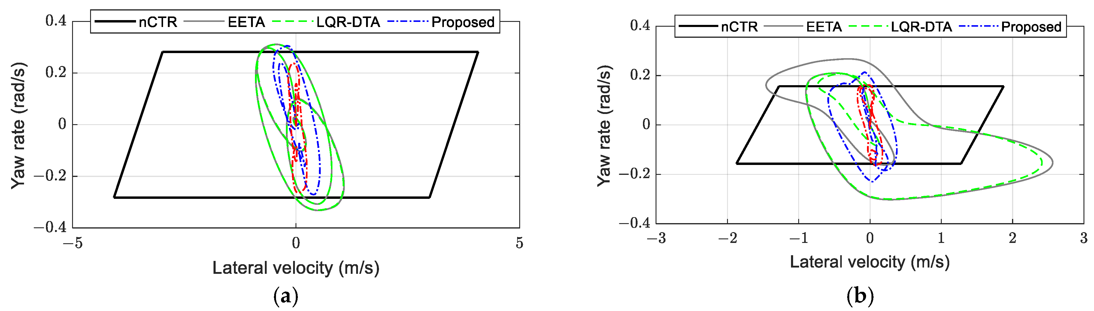
Combining Figure 9 and Figure 10 for analysis, under both scenarios, the smallest sideslip angle amplitude and the smallest driver’s front wheel steering angle input are realized by the proposed strategy, indicating the superior coordinated effects in vehicle handling and stability. Further, Figure 11 shows the phase plane state trajectories of each strategy under both DLC drive cycles. It can be observed that the trajectory of the proposed strategy is closer to the origin of the coordinate system, demonstrating the more desirable stability. Compared with the results for Case 1, under the more extreme conditions of Case 2, the trajectory variation ranges of the nCTR, EETA, and LQR-DTA methods increased significantly, reducing vehicle handling and stability. However, owing to the proposed strategy’s ability to assess vehicle stability in real time, determine handling and stability coordination references, and achieve the expected reference tracking accuracy, it exhibited similar phase trajectory performance in Case 2 to that in Case 1.

4.3. Index Analysis of Handling, Stablity, Energy Efficency, and Computation

To comprehensively validate the performance, this section further evaluates handling, stability, energy consumption, and computation time, with the following quantitative indexes defined:

• Handling Indicator:

$$I_{\mathrm{h}\mathrm{a}\mathrm{n}\mathrm{d}\mathrm{l}\mathrm{i}\mathrm{n}\mathrm{g}}=\int \left|\delta \right|\mathrm{d}t$$

(36)

For a vehicle with desirable handling, the driver requires less operational/working load to achieve the expected vehicle behavior. Therefore, the handling is assessed by the integral of the absolute value of the driver’s front wheel steering angle with respect to time. A smaller value of $I_{\mathrm{h}\mathrm{a}\mathrm{n}\mathrm{d}\mathrm{l}\mathrm{i}\mathrm{n}\mathrm{g}}$ indicates better vehicle handling.

2.

Stability Indicator:

$$I_{\mathrm{s}\mathrm{t}\mathrm{a}\mathrm{b}\mathrm{i}\mathrm{l}\mathrm{i}\mathrm{t}\mathrm{y}}=\int \iota \mathrm{d}t$$

(37)

As described in Section 3.2, when the vehicle is at risk of instability or has already lost stability, the adjustable factor $\iota$ will increase to 1. Thus, vehicle stability can be evaluated using (37). That is, a smaller value of $I_{\mathrm{s}\mathrm{t}\mathrm{a}\mathrm{b}\mathrm{i}\mathrm{l}\mathrm{i}\mathrm{t}\mathrm{y}}$ indicates better vehicle stability.

3.

Energy Consumption Indicator:

$$I_{\mathrm{e}\mathrm{n}\mathrm{e}\mathrm{r}\mathrm{g}\mathrm{y}}=\int P_{\mathrm{m}\mathrm{i}}\mathrm{d}t$$

(38)

The energy consumption is evaluated by the integral of the sum of the internal powers of the vehicle’s four IWMs in terms of time.

Based on the above three indexes, the results of each strategy under Case 1 and Case 2 conditions were calculated and are illustrated in Figure 12. In both cases, the proposed strategy illustrated the optimum performance in handling, stability, and energy consumption. Instead, nCTR, which uses an equal TA approach, performed poorly on all indicators. In particular, the LQR-DTA strategy showed higher values for energy consumption and stability indexes under Case 1 conditions. This was mainly because, firstly, handling and stability were generally conflicting, and under this scenario, LQR-DTA prioritizes handling at the cost of energy consumption; and secondly, although the DTA TA method contributes to energy savings, it does not explicitly optimize energy consumption minimization as in the proposed strategy, leaving room for further energy-saving potential.

Furthermore, if $1/I_{\mathrm{e}\mathrm{n}\mathrm{e}\mathrm{r}\mathrm{g}\mathrm{y}}$ is taken as an indicator to roughly compare the AER mileages, and the AER of the proposed strategy is considered as the unit value of 1, then the results for the nCTR, EETA, and LQR-DTA strategies under Case 1 and Case 2 are respectively as follows. (1) Case 1: 0.9174, 0.9737, and 0.9083; (2) Case 2: 0.7758, 0.8734, and 0.9191. That is, assuming the vehicle operates under Case 1 and Case 2 conditions for an extended period, the proposed strategy improved the AER mileage by more than 2.63% and 8.09% compared with the other strategies, with maximum improvements of 9.17% and 22.42% (compared with nCTR and LQR-DTA, which only consider handling–stability control). Given the above, the proposed strategy can effectively enhance the motor energy efficiency of DDEVs, contributing to an increase in the vehicle’s AER.

Figure 13 presents the single-step CPU computation time results of the proposed strategy under Case 1 and Case 2. In both cases, the computation time for both the upper and lower layers of the proposed strategy was less than 0.008 s, and most of the time, it took only about 0.003 s or less, demonstrating high computational efficiency. Specifically, before 2 s in both cases, the computation time in upper and lower layers was relatively low. This is primarily because the vehicle is traveling in the straight-line phase of the DLC at this stage, resulting in no error in the yaw rate reference tracking for the upper layer, and meanwhile in the lower layer, the changes in the vehicle’s generalized control forces are not significant. Thus, the number of optimization iterations for two layers is low, leading to short computation times. Quantitatively,

Table 2. Calculation time of proposed strategy.

Drive Cycle	Layer	Calculation Time
		Maximum	Mean
Case 1	Upper (MPC)	0.0068 s	0.0025 s
	Lower (TA)	0.0042 s	0.0011 s
Case 2	Upper (MPC)	0.0066 s	0.0025 s
	Lower (TA)	0.0032 s	0.001 s

lists the CPU computation times for the upper and lower layers of the proposed strategy. Under both Case 1 and Case 2 conditions, the computation time for each control period of the proposed strategy’s upper and lower layers was less than the sampling time of 0.02 s. This is primarily because the optimization problems in both the upper and lower control layers are formulated as convex optimization problems, ensuring high computational efficiency. In summary, the proposed strategy in this paper demonstrates favorable potential for real-time application.

5. Conclusions

This paper introduces a coordinated control strategy for DDEVs equipped with ARS and DYC, with the objective of enhancing handling performance, stability, and energy economy. An analytical expression, derived from the front wheel steering angle, delineated the stability boundary. Furthermore, an adjustment factor was introduced to quantify the current vehicle stability status, serving as a reference for optimal coordination in handling and stability control. At the upper-level motion control layer, an MPC approach was employed to track this reference and implement both ARS and DYC. Specifically, the rear lateral force was utilized as the control command, which was then converted into a rear wheel steering angle using a predefined tire inverse model. Meanwhile, the front lateral force was modeled as an LTV system to enhance computational efficiency in the MPC optimization process. At the TA layer, the adjustment factor was leveraged to balance tire workload rate and IWMs’ energy consumption, enabling seamless transitions between energy consumption optimization and driving stability targets. Notably, both the upper and lower-level optimization problems presented in this paper are convex, facilitating efficient solution methodologies. Simulation results validated the effectiveness of the proposed strategy under various road adhesion conditions, demonstrating improved coordination among handling, stability, and energy efficiency in a computationally efficient manner.

The results indicate that the proposed yaw rate reference can effectively maintain stability requirements when the vehicle approaches instability, thanks to the specifically designed stability bounds, adjustable factor, and weight coefficient. When compared with the nCTR, EETA, and LQR-DTA methods, the proposed strategy exhibited superior performance in tracking the yaw rate reference with minimal errors and achieved the smallest sideslip angle under both Case 1 and Case 2, thereby demonstrating superior driving handling and stability. In terms of the evaluated indexes, the proposed strategy also yielded optimal results in handling, stability, and energy efficiency among the four methods. Specifically, the rough comparisons between AER mileage were conducted for Case 1 and Case 2 conditions, and the proposed strategy improved the AER mileage by more than 2.63% and 8.09% compared with others, with maximum improvements of 9.17% and 22.42%, respectively. Therefore, the proposed strategy significantly enhances the motor energy efficiency of DDEVs compared with methods that only consider handling and stability control, thereby benefiting to extending the AER mileage. Additionally, the maximum computational time per sample step for the proposed strategy was around 0.0065 s for the upper-level MPC and 0.004 s for the lower-level TA, significantly less than the sample time of 0.02 s, suggesting its potential for real-time application.

Future work will primarily focus on enhancing the robustness of the control algorithm. Considering the upper and lower-layer architecture presented in this paper, to improve the robustness of the controller in scenarios involving sensor disturbances, vehicle model errors, and other factors, robust control methods such as tube MPC and H-infinity methods can be developed for the upper layer targeting DYC issues, while robust control allocation methods can be employed in the lower layer for torque distribution design. Additionally, to adapt to the trend of vehicle intelligence and autonomy, plans are in place to expand and further refine the proposed strategy by incorporating application scenarios such as vehicle-to-vehicle (V2V) communication and autonomous driving.