
Ecological Restoration and Zonal Management of Degraded Grassland Based on Cost–Benefit Analysis: A Case Study in Qinghai, China


Abstract
:1. Introduction
2. Study Area and Data
2.1. Study Area
2.2. Data Sources
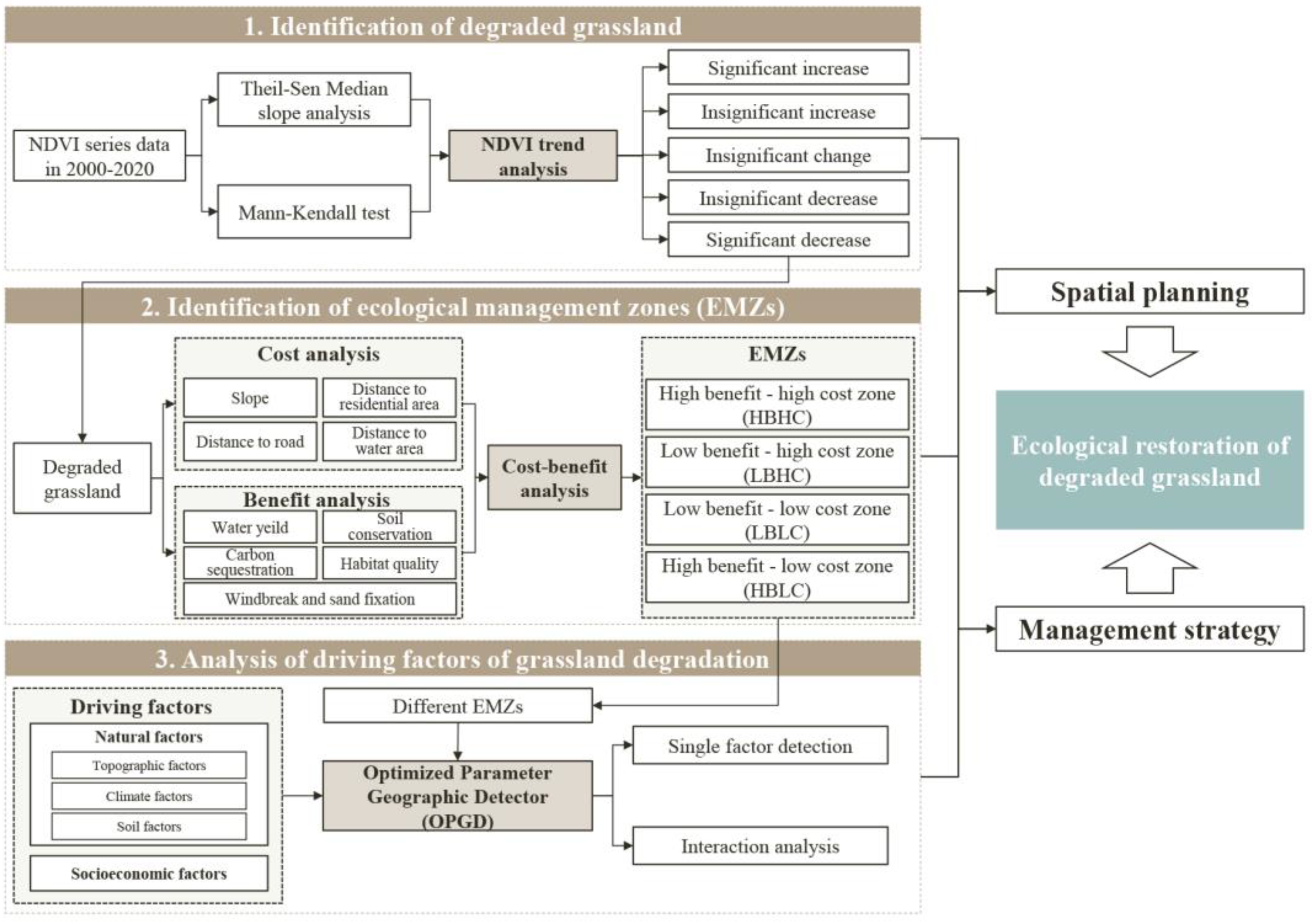
3. Methods
3.1. NDVI Trend Analysis of Grasslands
3.2. Identification of EMZs Based on Cost–Benefit Analysis
3.2.1. Cost Analysis
3.2.2. Benefit Analysis
3.2.3. Identification of EMZs
3.3. Analysis of Driving Factors for Grassland Degradation Using OPGD
3.3.1. Selection of Driving Factors
3.3.2. OPGD Model
4. Result
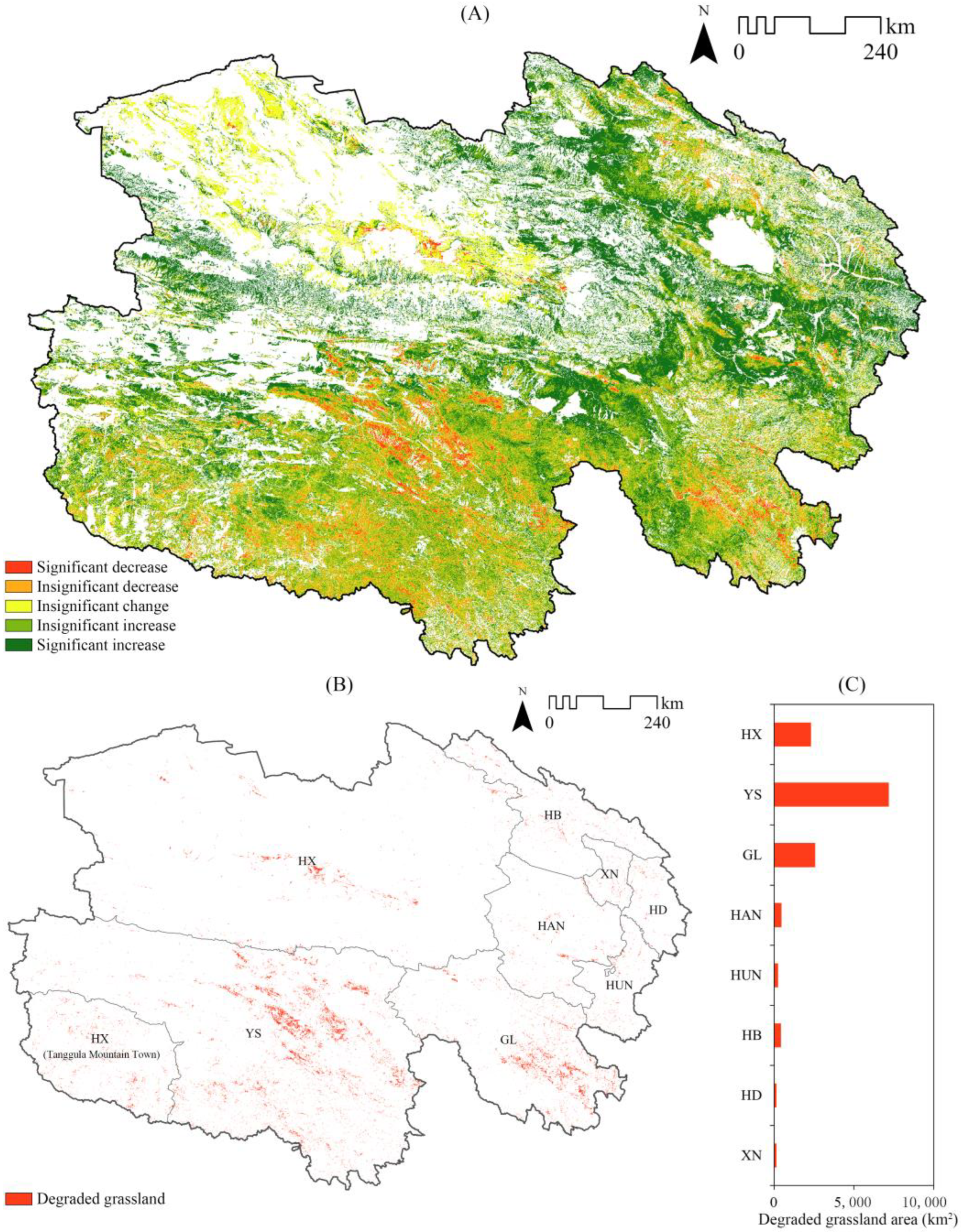
4.1. Identification of Degraded Grasslands
4.1.1. Trends of Grassland NDVI
4.1.2. Spatial Distribution of Degraded Grasslands
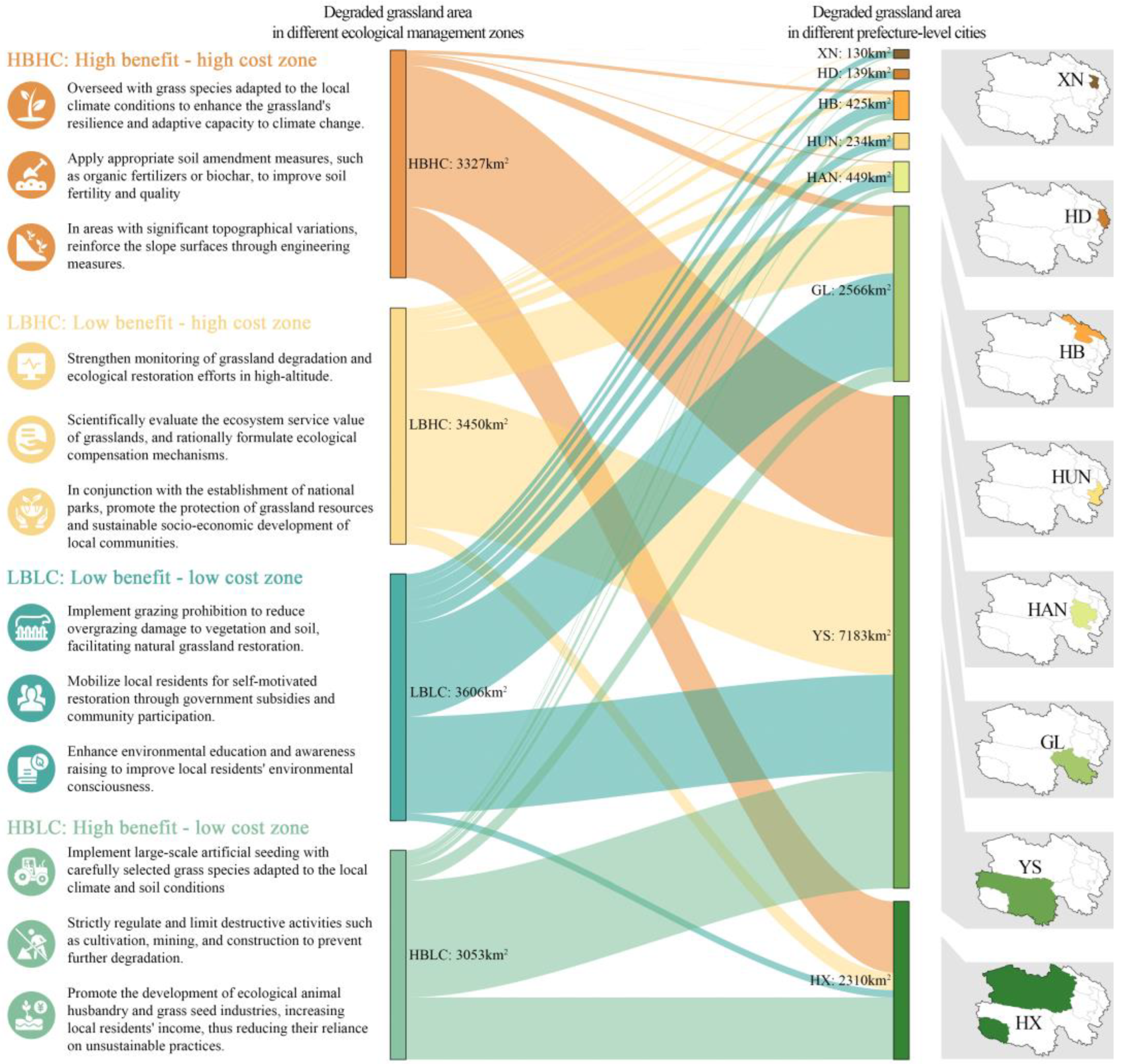
4.2. Identification of EMZs for Degraded Grasslands
4.2.1. EMZs for Degraded Grasslands Based on Cost–Benefit Analysis
4.2.2. Distribution of EMZs in Different Prefecture-Level Cities
4.3. Analysis of Driving Factors of Grassland Degradation in Different EMZs
4.3.1. The Impact of Different Driving Factors on Grassland Degradation
4.3.2. Interaction of Driving Factors
5. Discussion
5.1. Comparison of the Impact of Driving Factors on Grassland Degradation
5.2. Insights for Spatial Planning and Management Strategies for Degraded Grasslands
5.3. Strengths, Limitations, and Future Directions
6. Conclusions
Supplementary Materials
Author Contributions
Funding
Data Availability Statement
Conflicts of Interest
References
- O’Mara, F.P. The role of grasslands in food security and climate change. Ann. Bot. 2012, 110, 1263–1270. [Google Scholar] [CrossRef] [PubMed]
- Wilsey, B.J. The Biology of Grasslands; Oxford University Press: Oxford, UK, 2018. [Google Scholar]
- Du, Q.; Sun, Y.; Guan, Q.; Pan, N.; Wang, Q.; Ma, Y.; Li, H.; Liang, L. Vulnerability of grassland ecosystems to climate change in the Qilian Mountains, northwest China. J. Hydrol. 2022, 612, 128305. [Google Scholar] [CrossRef]
- Raiesi, F.; Riahi, M. The influence of grazing exclosure on soil C stocks and dynamics, and ecological indicators in upland arid and semi-arid rangelands. Ecol. Indic. 2014, 41, 145–154. [Google Scholar] [CrossRef]
- Schaub, S.; Finger, R.; Leiber, F.; Probst, S.; Kreuzer, M.; Weigelt, A.; Buchmann, N.; Scherer-Lorenzen, M. Plant diversity effects on forage quality, yield and revenues of semi-natural grasslands. Nat. Commun. 2020, 11, 768. [Google Scholar] [CrossRef]
- Bao, T.; Xi, G. Impact of grassland storage balance management policies on ecological vulnerability: Evidence from ecological vulnerability assessments in the Selinco region of China. J. Clean. Prod. 2023, 426, 139178. [Google Scholar] [CrossRef]
- Ye, T.; Liu, W.; Chen, S.; Chen, D.; Shi, P.; Wang, A.; Li, Y. Reducing livestock snow disaster risk in the Qinghai–Tibetan Plateau due to warming and socioeconomic development. Sci. Total Environ. 2022, 813, 151869. [Google Scholar] [CrossRef]
- Dong, S. Revitalizing the grassland on the Qinghai–Tibetan Plateau. Grassl. Res. 2023, 2, 241–250. [Google Scholar] [CrossRef]
- Wang, S.; Dai, E.; Jia, L.; Wang, Y.; Huang, A.; Liao, L.; Cai, L.; Fan, D. Assessment of multiple factors and interactions affecting grassland degradation on the Tibetan Plateau. Ecol. Indic. 2023, 154, 110509. [Google Scholar] [CrossRef]
- Li, C.; de Jong, R.; Schmid, B.; Wulf, H.; Schaepman, M.E. Changes in grassland cover and in its spatial heterogeneity indicate degradation on the Qinghai-Tibetan Plateau. Ecol. Indic. 2020, 119, 106641. [Google Scholar] [CrossRef]
- Zhou, W.; Yang, H.; Huang, L.; Chen, C.; Lin, X.; Hu, Z.; Li, J. Grassland degradation remote sensing monitoring and driving factors quantitative assessment in China from 1982 to 2010. Ecol. Indic. 2017, 83, 303–313. [Google Scholar] [CrossRef]
- Zhang, M.; Zhang, F.; Guo, L.; Dong, P.; Cheng, C.; Kumar, P.; Johnson, B.A.; Chan, N.W.; Shi, J. Contributions of climate change and human activities to grassland degradation and improvement from 2001 to 2020 in Zhaosu County, China. J. Environ. Manag. 2023, 348, 119465. [Google Scholar] [CrossRef] [PubMed]
- Wang, Z.; Wang, Y.; Liu, Y.; Wang, F.; Deng, W.; Rao, P. Spatiotemporal characteristics and natural forces of grassland NDVI changes in Qilian Mountains from a sub-basin perspective. Ecol. Indic. 2023, 157, 111186. [Google Scholar] [CrossRef]
- Gao, W.; Zheng, C.; Liu, X.; Lu, Y.; Chen, Y.; Wei, Y.; Ma, Y. NDVI-based vegetation dynamics and their responses to climate change and human activities from 1982 to 2020: A case study in the Mu Us Sandy Land, China. Ecol. Indic. 2022, 137, 108745. [Google Scholar] [CrossRef]
- Purevdorj, T.; Tateishi, R.; Ishiyama, T.; Honda, Y. Relationships between percent vegetation cover and vegetation indices. Int. J. Remote Sens. 1998, 19, 3519–3535. [Google Scholar] [CrossRef]
- Zhao, Y.; Chang, C.; Zhou, X.; Zhang, G.; Wang, J. Land use significantly improved grassland degradation and desertification states in China over the last two decades. J. Environ. Manag. 2024, 349, 119419. [Google Scholar] [CrossRef]
- Li, J.; Huang, L.; Cao, W.; Wang, J.; Fan, J.; Xu, X.; Tian, H. Benefits, potential and risks of China’s grassland ecosystem conservation and restoration. Sci. Total Environ. 2023, 905, 167413. [Google Scholar] [CrossRef]
- Liu, G.; Deng, X.; Zhang, F. The spatial and source heterogeneity of agricultural emissions highlight necessity of tailored regional mitigation strategies. Sci. Total Environ. 2024, 914, 169917. [Google Scholar] [CrossRef]
- Wang, Z.; Gao, Y.; Zhang, X.; Li, L.; Li, F. Integrating historical patterns and future trends for ecological management zone identification and validation: A case study in Beijing, China. Sci. Total Environ. 2024, 927, 172249. [Google Scholar] [CrossRef]
- Liu, G.; Zhang, F. Land zoning management to achieve carbon neutrality: A case study of the Beijing–Tianjin–Hebei urban agglomeration, China. Land 2022, 11, 551. [Google Scholar] [CrossRef]
- Shao, Q.; Liu, S.; Ning, J.; Liu, G.; Yang, F.; Zhang, X.; Niu, L.; Huang, H.; Fan, J.; Liu, J. Remote sensing assessment of the ecological benefits provided by national key ecological projects in China during 2000–2019. J. Geogr. Sci. 2023, 33, 1587–1613. [Google Scholar] [CrossRef]
- Cao, S.; Xia, C.; Suo, X.; Wei, Z. A framework for calculating the net benefits of ecological restoration programs in China. Ecosyst. Serv. 2021, 50, 101325. [Google Scholar] [CrossRef]
- Yin, R.; Yin, G. China’s primary programs of terrestrial ecosystem restoration: Initiation, implementation, and challenges. Environ. Manag. 2010, 45, 429–441. [Google Scholar] [CrossRef] [PubMed]
- Zhao, H.; Wei, D.; Wang, X.; Hong, J.; Wu, J.; Xiong, D.; Liang, Y.; Yuan, Z.; Qi, Y.; Huang, L. Three decadal large-scale ecological restoration projects across the Tibetan Plateau. Land Degrad. Dev. 2024, 35, 22–32. [Google Scholar] [CrossRef]
- Cao, S.; Liu, Y.; Su, W.; Zheng, X.; Yu, Z. The net ecosystem services value in mainland China. Sci. China Earth Sci. 2018, 61, 595–603. [Google Scholar] [CrossRef]
- Xu, D.; Wang, Y.; Wang, Z. Linking priority areas and land restoration options to support desertification control in northern China. Ecol. Indic. 2022, 137, 108747. [Google Scholar] [CrossRef]
- Zhao, Y.; Liu, S.; Liu, H.; Wang, F.; Dong, Y.; Wu, G.; Li, Y.; Wang, W.; Tran, L.-S.P.; Li, W. Multi-objective ecological restoration priority in China: Cost-benefit optimization in different ecological performance regimes based on planetary boundaries. J. Environ. Manag. 2024, 356, 120701. [Google Scholar] [CrossRef]
- Dong, Z.; Bian, Z.; Jin, W.; Guo, X.; Zhang, Y.; Liu, X.; Wang, C.; Guan, D. An integrated approach to prioritizing ecological restoration of abandoned mine lands based on cost-benefit analysis. Sci. Total Environ. 2024, 924, 171579. [Google Scholar] [CrossRef]
- Wang, H.; Tian, F.; Wu, J.; Nie, X. Is China forest landscape restoration (FLR) worth it? A cost-benefit analysis and non-equilibrium ecological view. World Dev. 2023, 161, 106126. [Google Scholar] [CrossRef]
- Lin, Y.; Chen, Q.; Huang, F.; Xue, X.; Zhang, Y. Identifying ecological risk and cost-benefit value for supporting habitat restoration: A case study from Sansha Bay, southeast China. Ecol. Process. 2023, 12, 20. [Google Scholar] [CrossRef]
- Wang, C.; Liu, Y.; Liu, X.; Qiao, W.; Zhao, M. Valuing ecological restoration benefits cannot fully support landscape sustainability: A case study in Inner Mongolia, China. Landsc. Ecol. 2023, 38, 3289–3306. [Google Scholar] [CrossRef]
- Bardgett, R.D.; Bullock, J.M.; Lavorel, S.; Manning, P.; Schaffner, U.; Ostle, N.; Chomel, M.; Durigan, G.; L Fry, E.; Johnson, D. Combatting global grassland degradation. Nat. Rev. Earth Environ. 2021, 2, 720–735. [Google Scholar] [CrossRef]
- Feng, Y.; Zhu, J.; Zhao, X.; Tang, Z.; Zhu, J.; Fang, J. Changes in the trends of vegetation net primary productivity in China between 1982 and 2015. Environ. Res. Lett. 2019, 14, 124009. [Google Scholar] [CrossRef]
- Liu, G.; Zhang, F. How do trade-offs between urban expansion and ecological construction influence CO2 emissions? New evidence from China. Ecol. Indic. 2022, 141, 109070. [Google Scholar] [CrossRef]
- Liu, X.; Zhang, J.; Zhu, X.; Pan, Y.; Liu, Y.; Zhang, D.; Lin, Z. Spatiotemporal changes in vegetation coverage and its driving factors in the Three-River Headwaters Region during 2000–2011. J. Geogr. Sci. 2014, 24, 288–302. [Google Scholar] [CrossRef]
- Li, Z.; Huffman, T.; McConkey, B.; Townley-Smith, L. Monitoring and modeling spatial and temporal patterns of grassland dynamics using time-series MODIS NDVI with climate and stocking data. Remote Sens. Environ. 2013, 138, 232–244. [Google Scholar] [CrossRef]
- Yan, H.; Ran, Q.; Hu, R.; Xue, K.; Zhang, B.; Zhou, S.; Zhang, Z.; Tang, L.; Che, R.; Pang, Z. Machine learning-based prediction for grassland degradation using geographic, meteorological, plant and microbial data. Ecol. Indic. 2022, 137, 108738. [Google Scholar] [CrossRef]
- Wang, J.F.; Li, X.H.; Christakos, G.; Liao, Y.L.; Zhang, T.; Gu, X.; Zheng, X.Y. Geographical detectors-based health risk assessment and its application in the neural tube defects study of the Heshun Region, China. Int. J. Geogr. Inf. Sci. 2010, 24, 107–127. [Google Scholar] [CrossRef]
- Du, Z.; Yu, L.; Chen, X.; Gao, B.; Yang, J.; Fu, H.; Gong, P. Land use/cover and land degradation across the Eurasian steppe: Dynamics, patterns and driving factors. Sci. Total Environ. 2024, 909, 168593. [Google Scholar] [CrossRef]
- Li, C.; Qiao, W.; Gao, B.; Chen, Y. Unveiling spatial heterogeneity of ecosystem services and their drivers in varied landform types: Insights from the Sichuan-Yunnan ecological barrier area. J. Clean. Prod. 2024, 442, 141158. [Google Scholar] [CrossRef]
- Song, Y.; Wang, J.; Ge, Y.; Xu, C. An optimal parameters-based geographical detector model enhances geographic characteristics of explanatory variables for spatial heterogeneity analysis: Cases with different types of spatial data. GIScience Remote Sens. 2020, 57, 593–610. [Google Scholar] [CrossRef]
- Li, S.; Yu, D.; Li, X. Exploring the impacts of ecosystem services on human well-being in Qinghai Province under the framework of the sustainable development goals. J. Environ. Manag. 2023, 345, 118880. [Google Scholar] [CrossRef] [PubMed]
- Li, X.L.; Perry, G.; Brierley, G.; Sun, H.Q.; Li, C.H.; Lu, G.X. Quantitative assessment of degradation classifications for degraded alpine meadows (heitutan), Sanjiangyuan, western China. Land Degrad. Dev. 2014, 25, 417–427. [Google Scholar] [CrossRef]
- Arrogante-Funes, P.; Osuna, D.; Arrogante-Funes, F.; Álvarez-Ripado, A.; Bruzón, A.G. Uncovering NDVI time trends in Spanish high mountain biosphere reserves: A detailed study. J. Environ. Manag. 2024, 355, 120527. [Google Scholar] [CrossRef] [PubMed]
- Ali, R.O.; Abubaker, S.R. Trend analysis using Mann-Kendall, Sen’s slope estimator test and innovative trend analysis method in Yangtze River basin, China. Int. J. Eng. Technol. 2019, 8, 110–119. [Google Scholar]
- Miyasaka, T.; Okuro, T.; Miyamori, E.; Zhao, X.; Takeuchi, K. Effects of different restoration measures and sand dune topography on short-and long-term vegetation restoration in northeast China. J. Arid Environ. 2014, 111, 1–6. [Google Scholar] [CrossRef]
- Cao, S. Impacts of China’s large-scale ecological restoration program on society and the environment. China Popul. Resour. Environ. 2012, 22, 101–108. [Google Scholar]
- Chen, J.; Wang, Y.; Sun, J.; Li, R.; Wang, Y.; Fu, Y.; Zhang, J.; Huo, H.; Liang, E. Cost-effective priorities for prefectural biodiversity and ecosystem service conservation planning on the Qinghai-Tibet Plateau. Ecol. Indic. 2023, 156, 111122. [Google Scholar] [CrossRef]
- Li, K.; Hou, Y.; Fu, Q.; Randall, M.T.; Andersen, P.S.; Qiu, M.; Skov-Petersen, H. Integrating decision-making preferences into ecosystem service conservation area identification: A case study of water-related ecosystem services in the Dawen River watershed, China. J. Environ. Manag. 2023, 340, 117972. [Google Scholar] [CrossRef]
- Li, K.; Hou, Y.; Andersen, P.S.; Xin, R.; Rong, Y.; Skov-Petersen, H. Identifying the potential areas of afforestation projects using cost-benefit analysis based on ecosystem services and farmland suitability: A case study of the Grain for Green Project in Jinan, China. Sci. Total Environ. 2021, 787, 147542. [Google Scholar] [CrossRef]
- Mao, C.; Ren, Q.; He, C.; Qi, T. Assessing direct and indirect impacts of human activities on natural habitats in the Qinghai-Tibet Plateau from 2000 to 2020. Ecol. Indic. 2023, 157, 111217. [Google Scholar] [CrossRef]
- Zhao, Z.; Dai, E. Vegetation cover dynamics and its constraint effect on ecosystem services on the Qinghai-Tibet Plateau under ecological restoration projects. J. Environ. Manag. 2024, 356, 120535. [Google Scholar] [CrossRef] [PubMed]
- Zhao, M.; Running, S.W. Drought-induced reduction in global terrestrial net primary production from 2000 through 2009. Science 2010, 329, 940–943. [Google Scholar] [CrossRef] [PubMed]
- Wackernagel, M.; Hanscom, L.; Jayasinghe, P.; Lin, D.; Murthy, A.; Raven, P. The importance of resource security for poverty eradication. Nat. Sustain. 2021, 4, 731–738. [Google Scholar] [CrossRef]
- Zhang, X.; Fan, H.; Sun, L.; Liu, W.; Wang, C.; Wu, Z.; Lv, T. Identifying regional eco-environment quality and its influencing factors: A case study of an ecological civilization pilot zone in China. J. Clean. Prod. 2024, 435, 140308. [Google Scholar] [CrossRef]
- Liu, L.; Zhang, Y.; Bai, W.; Yan, J.; Ding, M.; Shen, Z.; Li, S.; Zheng, D. Characteristics of grassland degradation and driving forces in the source region of the Yellow River from 1985 to 2000. J. Geogr. Sci. 2006, 16, 131–142. [Google Scholar] [CrossRef]
- Yuan, L.; Chen, X.; Wang, X.; Xiong, Z.; Song, C. Spatial associations between NDVI and environmental factors in the Heihe River Basin. J. Geogr. Sci. 2019, 29, 1548–1564. [Google Scholar] [CrossRef]
- Gong, X.; Li, Y.; Wang, X.; Zhang, Z.; Lian, J.; Ma, L.; Chen, Y.; Li, M.; Si, H.; Cao, W. Quantitative assessment of the contributions of climate change and human activities on vegetation degradation and restoration in typical ecologically fragile areas of China. Ecol. Indic. 2022, 144, 109536. [Google Scholar] [CrossRef]
- Ma, X.; Asano, M.; Tamura, K.; Zhao, R.; Nakatsuka, H.; Wang, T. Physicochemical properties and micromorphology of degraded alpine meadow soils in the Eastern Qinghai-Tibet Plateau. Catena 2020, 194, 104649. [Google Scholar] [CrossRef]
- Lai, C.; Li, C.; Peng, F.; Xue, X.; You, Q.; Zhang, W.; Ma, S. Plant community change mediated heterotrophic respiration increase explains soil organic carbon loss before moderate degradation of alpine meadow. Land Degrad. Dev. 2021, 32, 5322–5333. [Google Scholar] [CrossRef]
- Wei, D.; Zhao, H.; Zhang, J.; Qi, Y.; Wang, X. Human activities alter response of alpine grasslands on Tibetan Plateau to climate change. J. Environ. Manag. 2020, 262, 110335. [Google Scholar] [CrossRef]
- González-García, A.; Palomo, I.; González, J.A.; López, C.A.; Montes, C. Quantifying spatial supply-demand mismatches in ecosystem services provides insights for land-use planning. Land Use Policy 2020, 94, 104493. [Google Scholar] [CrossRef]
- Zhang, Y.; Zhao, X.; Gong, J.; Luo, F.; Pan, Y. Effectiveness and driving mechanism of ecological restoration efforts in China from 2009 to 2019. Sci. Total Environ. 2024, 910, 168676. [Google Scholar] [CrossRef] [PubMed]
- Guo, Y.; Li, R.; Yang, Y.; Ma, J.; Zheng, H. Integrating future grassland degradation risk to improve the spatial targeting efficiency of payment for ecosystem services. J. Environ. Manag. 2022, 317, 115490. [Google Scholar] [CrossRef] [PubMed]
- Liu, T.; Yu, L.; Chen, X.; Wu, H.; Lin, H.; Li, C.; Hou, J. Environmental laws and ecological restoration projects enhancing ecosystem services in China: A meta-analysis. J. Environ. Manag. 2023, 327, 116810. [Google Scholar] [CrossRef]
- Scotton, M. Mountain grassland restoration: Effects of sowing rate, climate and soil on plant density and cover. Sci. Total Environ. 2019, 651, 3090–3098. [Google Scholar] [CrossRef]


| Data Type | Data Format | Data Source | Spatial Resolution |
|---|---|---|---|
| Land use/land cover | Raster | RESDC. a | 30 m |
| Normalized Difference Vegetation Index | Raster | USGS. b | 500 m |
| Digital elevation model | Raster | GDCP. c | 1 km |
| Precipitation | Raster | RESDC. a | 1 km |
| Temperature | Raster | RESDC. a | 1 km |
| Evapotranspiration | Raster | RESDC. a | 1 km |
| Soil organic carbon | Raster | TPDC. d | 1 km |
| Cation exchange capacity | Raster | TPDC. d | 1 km |
| Clay fraction | Raster | TPDC. d | 1 km |
| GDP | Raster | RESDC. a | 1 km |
| Population density | Raster | RESDC. a | 1 km |
| Nighttime lighting index | Raster | TPDC. d | 1 km |
| Grazing intensity | Raster | TPDC. d | 1 km |
| Road, water area, residential area | Shapfile | NBGD. e | / |
| ES | Model | Calculation Method |
|---|---|---|
| Water yield | Water yield services are calculated using the Water Yield (WY) module of the InVEST model. | |
| where Y(x) is the annual water yield (mm); AET(x) is the annual actual evapotranspiration (mm); and p(x) is the annual precipitation (mm). | ||
| Carbon sequestration | As the basis of ecosystem material and the energy cycle, net primary productivity (NPP) can directly reflect the carbon storage capacity of vegetation [53]. This study uses NPP to represent carbon sequestration services. | The NPP data used in this study were obtained from the MOD17A3HGF annual composite datasets from the United States Geological Survey (www.usgs.gov). The datasets have a 500 m spatial resolution. |
| Soil conservation | Soil conservation services are calculated using the Sediment Delivery Ratio (SDR) module of the InVEST model. | |
| where SC is the actual soil conservation (t/ha); R is the rainfall erosivity (MJ·mm·(ha·h)−1); K is the soil erodibility (t·h·(MJ·mm)−1); LS is the slope length–gradient factor, which is calculated from the DEM data in the model with reference to the InVEST model manual; C is the vegetation cover management factor; and p is the support practice factor. | ||
| Habitat quality | Habitat-quality services are calculated by the Habitat Quality (HQ) module of the InVEST model. | |
| where Qxj is the habitat quality index of raster x in LULC type j; Hj is the habitat suitability of LULC type j; Dxj is the threatened degree of raster x in LULC type j; k is the half-saturation constant; and z is the model default value. | ||
| Windbreak and sand fixation | The Revised Wind Erosion Equation Model (RWEQ) can estimate regional soil wind erosion over extended time periods with high spatial and temporal resolution [28] and is used in this study to evaluate windbreak and sand fixation services. | |
| where WSF is annual sand fixation per unit area (kg/m2); SLQ is the potential amount of wind erosion of non-vegetation cover; and SL is the actual wind erosion. |
| Type | Driving Factors | Abbreviation | |
|---|---|---|---|
| Natural factors | Topographic factors | Altitude | ALT |
| Topographic relief index | TRI | ||
| Climate factors | Precipitation | PRE | |
| Temperature | TEM | ||
| Evapotranspiration | EVP | ||
| Soil factors | Soil organic carbon | SOC | |
| Cation exchange capacity | CEC | ||
| Clay content | CLAY | ||
| Socioeconomic factors | GDP | GDP | |
| Population density | POP | ||
| Nighttime lighting index | NLI | ||
| Grazing intensity | GRI | ||
Disclaimer/Publisher’s Note: The statements, opinions and data contained in all publications are solely those of the individual author(s) and contributor(s) and not of MDPI and/or the editor(s). MDPI and/or the editor(s) disclaim responsibility for any injury to people or property resulting from any ideas, methods, instructions or products referred to in the content. |
© 2024 by the authors. Licensee MDPI, Basel, Switzerland. This article is an open access article distributed under the terms and conditions of the Creative Commons Attribution (CC BY) license (https://creativecommons.org/licenses/by/4.0/).
Share and Cite
Wang, Z.; Li, F.; Xie, D.; Jia, J.; Cheng, C.; Lv, J.; Jia, J.; Jiang, Z.; Li, X.; Suo, Y. Ecological Restoration and Zonal Management of Degraded Grassland Based on Cost–Benefit Analysis: A Case Study in Qinghai, China. Sustainability 2024, 16, 11123. https://doi.org/10.3390/su162411123
Wang Z, Li F, Xie D, Jia J, Cheng C, Lv J, Jia J, Jiang Z, Li X, Suo Y. Ecological Restoration and Zonal Management of Degraded Grassland Based on Cost–Benefit Analysis: A Case Study in Qinghai, China. Sustainability. 2024; 16(24):11123. https://doi.org/10.3390/su162411123
Chicago/Turabian StyleWang, Ziyao, Feng Li, Donglin Xie, Jujie Jia, Chaonan Cheng, Jing Lv, Jianhua Jia, Zhe Jiang, Xin Li, and Yuxia Suo. 2024. "Ecological Restoration and Zonal Management of Degraded Grassland Based on Cost–Benefit Analysis: A Case Study in Qinghai, China" Sustainability 16, no. 24: 11123. https://doi.org/10.3390/su162411123
APA StyleWang, Z., Li, F., Xie, D., Jia, J., Cheng, C., Lv, J., Jia, J., Jiang, Z., Li, X., & Suo, Y. (2024). Ecological Restoration and Zonal Management of Degraded Grassland Based on Cost–Benefit Analysis: A Case Study in Qinghai, China. Sustainability, 16(24), 11123. https://doi.org/10.3390/su162411123