Article

WQI Improvement Based on XG-BOOST Algorithm and Exploration of Optimal Indicator Set

1
College of Architecture and Civil Engineering, Beijing University of Technology, Beijing 100124, China
2
Technical Centre for Soil, Agriculture and Rural Ecology and Environment, Ministry of Ecology and Environment, Beijing 100012, China
3
Hebei Institute of Water Resources, Shijiazhuang 050051, China
4
College of Water Sciences, Beijing Normal University, Beijing 100875, China
*
Authors to whom correspondence should be addressed.
Sustainability 2024, 16(24), 10991; https://doi.org/10.3390/su162410991
Submission received: 9 November 2024 / Revised: 9 December 2024 / Accepted: 11 December 2024 / Published: 14 December 2024

Abstract

:
This paper takes a portion of the Manas River Basin in Xinjiang Province, China, as an example and proposes an improved traditional comprehensive water quality index (WQI) method using Extreme Gradient Boosting (XG-BOOST) to analyze the groundwater quality levels in the region. Additionally, XG-BOOST is used to screen the existing dataset of ten water quality indicators, including fluoride (F), chlorine (Cl), nitrate (NO), sulfate (SO), silver (Ag), aluminum (Al), iron (Fe), lead (Pb), selenium (Se), and zinc (Zn), from 246 monitoring points, in order to find the dataset that optimizes model training performance. The results show that, in the selected study area, water quality categorized as “GOOD” and “POOR” accounts for the majority, with “GOOD” covering 48.7% of the area and “POOR” covering 31.6%. Regions with water quality classified as “UNFIT” are mainly distributed in the central–eastern parts of the study area, located in parts of the Changji Hui Autonomous Prefecture. Comparatively, water quality in the western part of the study area is better than that in the eastern part, while areas with “EXCELLENT” water quality are primarily distributed in the southern parts of the study area. The optimal water quality indicator dataset consists of five indicators: Cl, NO, Pb, Se, and Zn, achieving an accuracy of 98%, RMSE = 0.1414, and R2 = 0.9081.

1. Introduction

Groundwater resources have long been an important source of water supply and have become an important source of drinking water and domestic water for residents in urban and rural areas [1]. However, under the influence of unprecedented modernization, characterized by economic development, urbanization, and population explosion, groundwater resources are becoming more vulnerable to pollution [2]. Groundwater quality assessment is the basis of groundwater management and the key to controlling water pollution and improving water resources’ management.
Currently, there are numerous methods for groundwater quality assessment both domestically and internationally, which can mainly be divided into two categories: single-factor evaluation methods [3,4], and multi-factor comprehensive evaluation methods. As the name suggests, the single-factor evaluation methods evaluate groundwater quality based on only one indicator, comparing the selected indicator with its standard value. If the evaluation indicator exceeds its standard value, it indicates that the water sample does not meet the water quality requirements. Common single-factor evaluation methods include the mean value method, the extreme value method, and others. Although single-factor evaluation methods are simple to operate, they lack a comprehensive evaluation of all indicators, leading to less thorough assessment results. In contrast, multi-factor evaluation methods assign different weights based on the influence of each evaluation indicator on water quality and derive a comprehensive score, from which water quality assessment results are ranked and obtained. Common multi-factor evaluation methods include the Nemerow index method [5,6,7], comprehensive water quality index evaluation method, set pair analysis method [8,9], principal component analysis method [10], and so on.
In this paper, the comprehensive water quality index (WQI) method, a multi-factor evaluation method, was selected to evaluate groundwater quality, having been used by many researchers to evaluate groundwater quality in the study area. For instance, I. D. U. H. Piyathilake et al. [11] used the WQI method to assess and categorize the drinking water quality in Uva Province (UP), exploring the relationship between drinking water quality and the incidence of chronic kidney disease in the province. Frsat Abdullah Ababakr [12] and others used the WQI to evaluate groundwater quality and its variations in the city of Erbil, combining it with Geographic Information Systems (GISs) to map the spatial distribution of groundwater quality in the city, and analyzing the impact of kriging and Inverse Distance Weighting (IDW) interpolation methods on the final results. The results showed that kriging improved predictive accuracy compared to IDW. Asif Mahmud et al. [13] and M.M. Rahman et al. [14] also used the WQI method to investigate drinking water quality in the city of Khulna and five villages in Thakurgaon District, Bangladesh, and created spatial distribution maps. The WQI evaluation method assesses multiple groundwater quality indicators, providing a more comprehensive and reliable evaluation result. However, its calculation process is complex, and the indicator weighting process lacks objectivity, while the selection and weighting of indicators directly affect the rationality of the water quality evaluation. Recognizing this limitation, many researchers have chosen to combine the WQI method with other approaches to enhance the accuracy and reliability of evaluation results. Some scholars have combined the WQI with groundwater chemistry analysis methods for water quality assessment. For example, Mohamed Elsayed Gabr et al. [15] used a combination of WQI evaluation and groundwater chemistry methods (Gibbs diagram and Piper diagram) to study whether groundwater in the Dairut region of Upper Egypt is suitable for drinking and irrigation. Similarly, Gopal Krishan et al. [16] combined the WQI method with traditional hydrogeochemical analysis and ion ratio diagrams to analyze pre-monsoon and post-monsoon groundwater quality changes in the Mewat region of Haryana State, explaining and verifying the causes of groundwater quality changes through groundwater chemistry analysis. The results indicated that most groundwater in the region is unsuitable for drinking. Some researchers have utilized mathematical models to support WQI methods in regional water quality analysis. Md Galal Uddin et al. [17] employed a data-driven root mean square (RMS) model to evaluate groundwater quality near the Bay of Bengal in coastal Bangladesh, demonstrating that the RMS-WQI model exhibited minimal uncertainty in predicting WQI scores, effectively providing accurate assessments of global water quality in coastal areas. Akram Seif et al. [18] applied Monte Carlo simulations based on WQI evaluations, using posterior probability density functions (PDFs) to randomly generate weights and investigate uncertainties in the entire water quality index calculation process for the Kerman aquifer in Iran.
The WQI evaluation method assesses multiple groundwater quality indicators simultaneously, providing a more comprehensive and reliable evaluation result. The WQI evaluation method mainly consists of four steps: indicator selection, indicator scoring, indicator weighting, and aggregation. Among these, the selection of indicators and the determination of their weights are usually based on expert knowledge and experience. However, this can lead to subjectivity in determining the importance of water quality indicators, potentially overlooking indicators with greater influence. This lack of objectivity can affect the accuracy and reliability of the evaluation results, which, in turn, may reduce the effectiveness of groundwater management. In addition to combining the WQI with other methods to improve accuracy, researchers have also focused on the rapid development of artificial intelligence and computer technology in recent years to address the deficiencies of the WQI evaluation method itself. Machine learning (ML) offers advantages such as high computational speed, the ability to replace manual processing of large datasets, independence from complete physical and chemical mechanisms, and spatiotemporal continuous prediction, making it a promising approach for improving traditional WQI-based water quality assessment methods [19,20,21,22]. Xin Wang et al. [23] developed a WQI–Bayesian Model Averaging (BMA) model based on Bayesian methods, integrating multiple WQI models for comprehensive groundwater quality evaluation, and used the extreme gradient boosting algorithm to systematically assign weights to sub-indicator functions and calculate aggregate functions, thus avoiding the time and computational costs of parameter optimization. S. Vijay et al. [24] combined the WQI evaluation method with artificial neural networks to predict water quality indices for water samples collected from 1,944 different wells around the Vellore region, reducing manual computation time while improving accuracy. A. Gibrilla et al. [25] studied the groundwater quality of Birimian rocks, Cape Coast granites, and the Densu River using the WQI and multivariate statistical methods to determine their suitability for drinking and irrigation. Their study used cluster analysis and principal component analysis with varimax rotation as tools to verify and explain the chemical characteristics of the water quality. In this study, concentration data for ten indicators, including fluoride (F), chlorine (Cl), nitrate (NO), sulfate (SO), silver (Ag), aluminum (Al), iron (Fe), lead (Pb), selenium (Se), and zinc (Zn), from 246 monitoring points in the research area, were used to calculate the water quality index at each point using an XG-BOOST improved WQI model. A spatial distribution map of the water quality index was created with the help of GISs, and the optimal water quality indicator dataset for the research area was selected based on model performance. The novel contributions of this study are as follows:
(1)
Recent studies combining machine learning with the WQI evaluation method for water quality assessment have primarily focused on surface water quality in rivers and lakes. Research on groundwater quality using similar approaches is still evolving. This study evaluated the groundwater quality in a portion of the Manas River Basin in Xinjiang using an XG-BOOST improved WQI model, providing a reference for similar groundwater quality assessments.
(2)
The weight determination process in the XG-BOOST improved WQI model was replaced by machine algorithms, reducing reliance on experts and experience, and decreasing the likelihood of important indicators being overlooked due to subjective weighting. This improved the objectivity of the evaluation.
(3)
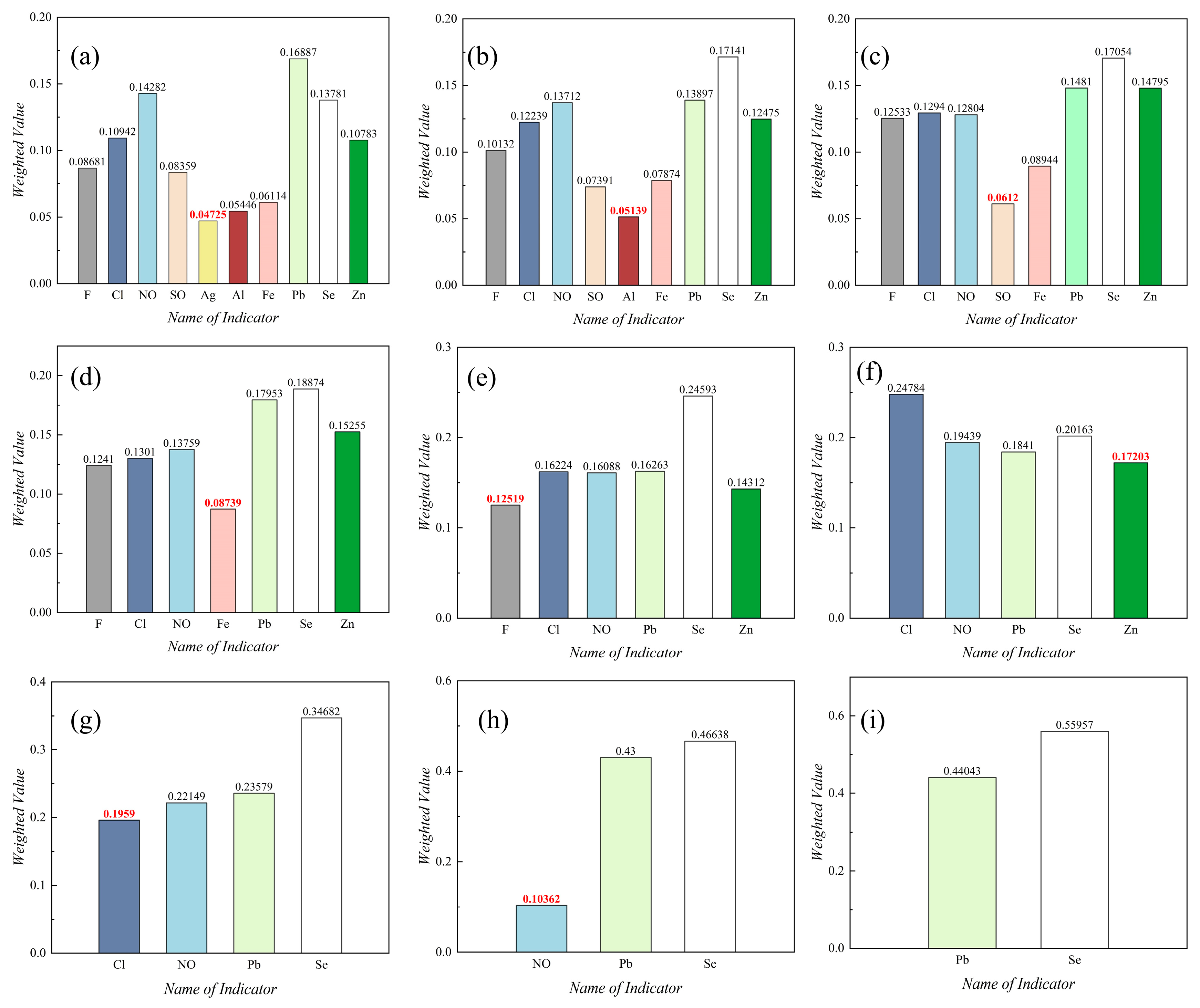
Using XG-BOOST to screen the ten water quality indicators in the study area, removing the indicator with the lowest weight value in each iteration, and observing its impact on the evaluation results and the prediction model. This process helps identify the optimal indicator dataset that maximizes model performance. This approach can explore the impact of indicator selection on the simulation results of the XG-BOOST model and the water quality evaluation outcomes.
(4)
The Manas River Basin is located in the northwest of China, within an arid climate zone. Groundwater is the main water source for daily life, production, and agricultural irrigation in the Xinjiang Manas River Basin. Due to the regional environmental background and long-term human activities, groundwater pollution is severe. Therefore, assessing the groundwater quality in this region is crucial for developing groundwater protection measures and has significant importance for the rational planning, management, and utilization of local groundwater resources.

2. Materials and Methods

2.1. Study Area Description

The study area of this research was selected from part of the Manas River Basin in Xinjiang Province. It was obtained by checking the map according to the area where the selected monitoring sites are located. This is because of the limitation of the monitoring sites, and if the whole basin was taken as the study area, it would lead to the over-concentration of the monitoring sites, which would ultimately result in a large deviation from the actual situation through the interpolation by GIS. The locations of the specific study areas are shown in Figure 1a,b.
The Manas River Basin is located at 84°44′~86°50′ E and 43°4′~46°0′ N, situated on the southern edge of the Junggar Basin. It extends eastward from the Taxi River to the Anjihai River in the west, originating in the Tianshan Mountains to the south and flowing northward into the desert. The overall terrain slopes from south to north and is divided into three zones: the southern mountainous and hilly area, the central oasis plain area, and the northern desert area [26]. The Manas River Basin has a mid-temperate continental arid climate, characterized by strong evaporation and low precipitation. Annual precipitation increases with elevation, and the average annual temperature ranges from 5.0 to 7.5 °C. The Manas River is the largest inland river in terms of water volume and length in the Junggar Basin, and its tributary-formed deltas have been extensively cultivated into farmland.
The Manas River Basin is located in the piedmont depression zone of the northern Tianshan Fold Belt, mainly consisting of Quaternary Upper Pleistocene and Holocene basins, with widespread distribution of bedrock, sandy conglomerates, clay, and siltstone throughout the basin. The general flow direction of surface water and groundwater in the Manas River Basin is from south to north, and the hydrogeological conditions are distinctly zonal, influenced by topography, geological structure, and stratigraphic lithology. The mountainous areas are mainly characterized by bedrock fissure water, primarily recharged by glacial meltwater and rainfall. From alluvial fans to alluvial plains, the dominant water type is Quaternary loose rock pore water, mainly recharged by vertical infiltration of surface runoff, and it discharges into downstream plains in the form of subsurface flow [26]. South of National Highway 312, the piedmont plain has a single-structure unconfined aquifer composed of coarse sand and gravel, featuring a rich pore structure and good permeability. North of the highway, the low plain area has a multi-layer structure of unconfined and confined aquifers, with unconfined aquifers and shallow confined aquifers within a depth of 100 m, and deep confined aquifers below 100 m, predominantly consisting of gravel, cobbles, sand and gravel, or sand layers [27].

2.2. Data Sources

This study originated from the application of key technologies for constructing ecological security patterns and risk control in the Luanhe River Basin to the Manas River Basin in Xinjiang. After the study commenced, groundwater sampling was conducted in the Manas River Basin, resulting in the acquisition of water quality indicator data for this research. The data include the concentration of ten indicators—F, Cl, NO, SO, Ag, Al, Fe, Pb, Se, and Zn—from 246 monitoring points in the Manas River Basin. The specific locations of the monitoring points are shown in Figure 1c.

2.3. WQI Evaluation Method

The WQI evaluation includes the following four main steps: (1) the process of water quality indicator selection, (2) the process of sub-indicator evaluation, (3) the process of water quality indicator assignment, and (4) the process of aggregating and calculating the water quality index.

2.3.1. Indicator Selection

Ten water quality indicators, F, Cl, NO, SO, Ag, Al, Fe, Pb, Se, and Zn, were selected for this study at all of the monitoring sites. The specifics on the screening of the indicators are described in Section 2.5 (Screening of the Optimal Set of Water Quality Indicators).

2.3.2. Sub-Indicator Evaluation

In this study, the sub-indicator evaluation scores are calculated by the following equation [28]:
C i j = ( V i j P i j ) × 100
where i denotes the ith monitoring location, j denotes the jth water quality indicator, C denotes the evaluation score of each sub-indicator, Vij denotes the concentration data of the jth water quality indicator at the ith testing location, and Pj denotes the maximum allowable value of the jth water quality indicator.
The maximum allowable value of each indicator in this study is based on the “Standards for Drinking Water Quality” (GB 5749-2022 [29]); the specific maximum allowable value of each water quality indicator in the standard is shown in Table 1.
During the data processing, it was found that some water quality indicators had undetected concentration values. In such cases, the concentration value for the indicator at the monitoring point was replaced with the maximum allowable concentration value for that indicator as specified in Table 1.

2.3.3. Water Quality Indicator Assignment

The traditional process of assigning water quality indicators relies on expert knowledge and experience and lacks objectivity. In this study, the XG-BOOST algorithm was used to assign water quality indicators, and the specific principles of the methodology are described in Section 2.4 (XG-BOOST Model).

2.3.4. Water Quality Indices Aggregation

Aggregation refers to the process of aggregating all of the water quality indicators of a monitoring site according to the scores and weights of the sub-indicators through the aggregation function to obtain the water quality index of the monitoring site. The aggregation function of this study is shown in the following formula:
W Q I i = j = 1 n C i j w j ,
where WQI denotes the water quality index obtained from aggregation, i denotes the ith monitoring site, j denotes the jth water quality indicator, n denotes the number of water quality indicators, Cij denotes the indicator score of the jth water quality indicator at the ith monitoring site, and w denotes the weight of the water quality indicator.
After calculation, the water quality indices for the 246 monitoring points were obtained. Using GISs, spatial interpolation was then performed to generate a spatial distribution map of the water quality indices for the study area. The interpolated water quality indices were then classified into different levels, with the specific index intervals and levels shown in Table 2 [28].

2.4. XG-BOOST Model

The AUC-ROC (Area Under the Receiver Operating Characteristic Curve) is an evaluation parameter that reflects the learning performance of a model. The closer the AUC is to 1, the better the model’s performance, as it correctly predicts 0 as 0 and 1 as 1. The closer the AUC is to 0, the more the model tends to predict 0 as 1 and 1 as 0. In fact, an AUC value closer to 0 or 1 clearly reflects the relationship between predicted and true values. However, when the AUC = 0.5, the model has the worst performance, as it lacks the ability to distinguish between classes. Using the AUC as the comparison standard, the learning performance of four machine learning models—XG-BOOST, Support Vector Machine (SVM), Random Forest, and Decision Tree—was compared based on the original dataset (which includes water quality data from 246 monitoring points with ten water quality indicators). The results were as follows: XG-BOOST: AUC = 0.91, Support Vector Machine: AUC = 0.87, Random Forest: AUC = 0.87, Decision Tree: AUC = 0.85, indicating that XG-BOOST had the best learning performance in this study. Therefore, based on the dataset used in this research, the XG-BOOST algorithm was selected to improve the traditional WQI water quality evaluation method.

2.4.1. Model Inputs

The concentration values of each water quality indicator from the 246 monitoring points were used as inputs for the XG-BOOST model. Additionally, water quality status was used as another input item. Determining the water quality status of each monitoring point involves comparing the concentration data of each indicator at the point with the maximum allowable concentration values in Table 1. If the concentrations of all monitored indicators at a point are below the maximum allowable values, the water quality status input for that point is assigned a binary value of “0”, indicating “unpolluted”. If at least one water quality indicator at a point has a concentration exceeding the maximum allowable value, the water quality status input for that point is assigned a binary value of “1”, indicating “polluted” [30]. Detailed input data, including the concentration values of the ten water quality indicators and the water quality status for the 246 monitoring points, are provided in the Supplementary Materials (Table S1).

2.4.2. Model Validation

The XG-BOOST model requires different training and testing groups during its operation. The purpose of the training group is to establish the relationship between the input water quality indicator concentrations and the water quality status, while the testing group uses the relationship learned through machine learning to predict the water quality status based on the water quality indicator concentrations. The predicted values are then compared with the actual values to evaluate the model’s learning effectiveness. In this study, the input data were randomly divided into two groups: 80% of the monitoring station input data served as the training group, and 20% as the testing group. The simplest way to evaluate model performance is by using a single training dataset and a single testing dataset. However, this can lead to high variance and overfitting [30]. Overfitting is a major problem in machine learning algorithms, where the model learns too well on the training data, capturing noise and random fluctuations rather than the underlying true relationships, resulting in poor performance on new, unseen data. Causes of overfitting may include excessive model complexity, a small amount of training data, and high data noise, among others.

2.4.3. Model Evaluation Criteria

After completing the training and testing of the XG-BOOST model, it is necessary to evaluate the model’s performance and effectiveness, which typically relies on several metrics. In this study, the root-mean-square error (RMSE), coefficient of determination (R-squared, R2), and accuracy were calculated based on the model inversion results. RMSE represents the root-mean-square error between the predicted values and the actual values, providing a more intuitive measure of error: the smaller the value, the better. R2 describes the proportion of variance in the dependent variable that is explained by the model, with values ranging between 0 and 1; the closer to 1, the better the model’s fit [31]. Accuracy refers to the degree to which the predicted water quality status from the testing group matches the actual values based on the relationships learned from the training group. The closer this value is to 100%, the better the model’s learning and prediction accuracy. The methods for calculating RMSE and R2 are shown in the following formulae [31]:
R M S E = 1 n i = 1 n ( y i y ^ i ) 2 ,
R 2 = 1 i = 1 n ( y i y ^ i ) 2 i = 1 n ( y i y ¯ ) 2 ,
where n denotes the number of input data, yi denotes the true value, y ^ i is the predicted value of the model, and y ¯ denotes the mean value.
Another metric is the AUC-ROC (Area Under the Receiver Operating Characteristic Curve), which measures the performance of a classification problem at various threshold settings. The ROC curve is a probability curve, and the AUC indicates the degree of separability. The closer the AUC is to 1, the better the model’s performance, meaning it can predict 0 as 0 and 1 as 1. Conversely, an AUC close to 0 indicates that the model is closer to predicting 0 as 1 and 1 as 0. In fact, AUC values closer to 0 or 1 clearly reflect the relationship between the predicted values and the actual values. However, when the AUC = 0.5, the model performs poorly because it has no discriminative capability.
Additionally, the training loss curve (LOSS curve) is an important tool for evaluating the training effectiveness of a machine learning model. By observing the LOSS curve, it is possible to determine whether the model is learning correctly and whether overfitting or underfitting issues are present. If the loss value gradually decreases as the training iterations increase, it usually indicates that the model is learning effectively and the training is proceeding well. If the LOSS curve fluctuates or stops decreasing, it may suggest overfitting or an unstable training process. If the loss value continues to decrease for the training set but begins to increase for the validation set, it indicates overfitting. If both the training and validation set loss values remain high, it suggests underfitting, and further model adjustments are needed.
In summary, after one iteration using XG-BOOST, five standard parameters for evaluating the learning performance of the model can be obtained: RMSE, R2, accuracy, AUC, and LOSS. When RMSE is smaller, R2 is larger, accuracy is higher, the AUC is closer to 0 or 1, and LOSS gradually decreases with minimal fluctuations, it indicates that the model’s learning performance in this iteration has reached its best. In other words, the water quality indicator set at this point is the optimal indicator dataset that achieves the best learning performance for the model.

2.4.4. Determination of Indicator Weights

XG-BOOST is an improved version of the Gradient Boosting Decision Tree (GBDT) and operates on similar principles. Both work by building decision trees and integrating the multiple decision trees obtained from training. The primary difference lies in the definition of the objective function. XG-BOOST introduces the concept of decision tree complexity into the GBDT loss function. The formula for its objective function is as follows:
O b j ( t ) = i = 1 n l ( y i , y ^ i ) + i = 1 t Ω ( f t ) ,
y ^ i ( t ) = t = 1 t f t ( x i ) ,
y ^ i ( t ) = y ^ i ( t 1 ) + f t ( x i ) ,
where obj is the XG-BOOST objective function, f t ( x i ) is the output of the tth tree, y ^ i ( t ) is the current output of the model, y i is the actual result, l is the LOSS function, i = 1 t Ω ( f t ) is the complexity of the number, i denotes the ith tree, n denotes that a total of n decision trees were trained, and t denotes that the current output is the tth tree.
By incorporating complexity into the objective function, removing constant terms, and applying the second-order Taylor expansion, the final simplified and optimized objective function is given by the following formula:
O b j ( t ) = j = 1 T [ G j w j + 1 2 ( H j + λ ) w j 2 ] + γ T ,
where T is the number of leaf nodes of the decision tree; G j denotes the cumulative sum of first-order partial derivatives of the samples contained in leaf node j, a constant; H j denotes the cumulative sum of second-order partial derivatives of the samples contained in leaf node j, a constant; w j denotes the value of the weights of leaf node j; and λ and γ are both parameters at the time of the model input.
According to the above equation, it can be seen that the weight value of the leaf node is the optimal solution for solving the quadratic equation, which can be obtained according to the rooting formula or after the first-order derivation.
w j = G j H j + λ
The above is the principle of XG-BOOST to calculate the weight value of each water quality indicator to influence the water quality status.

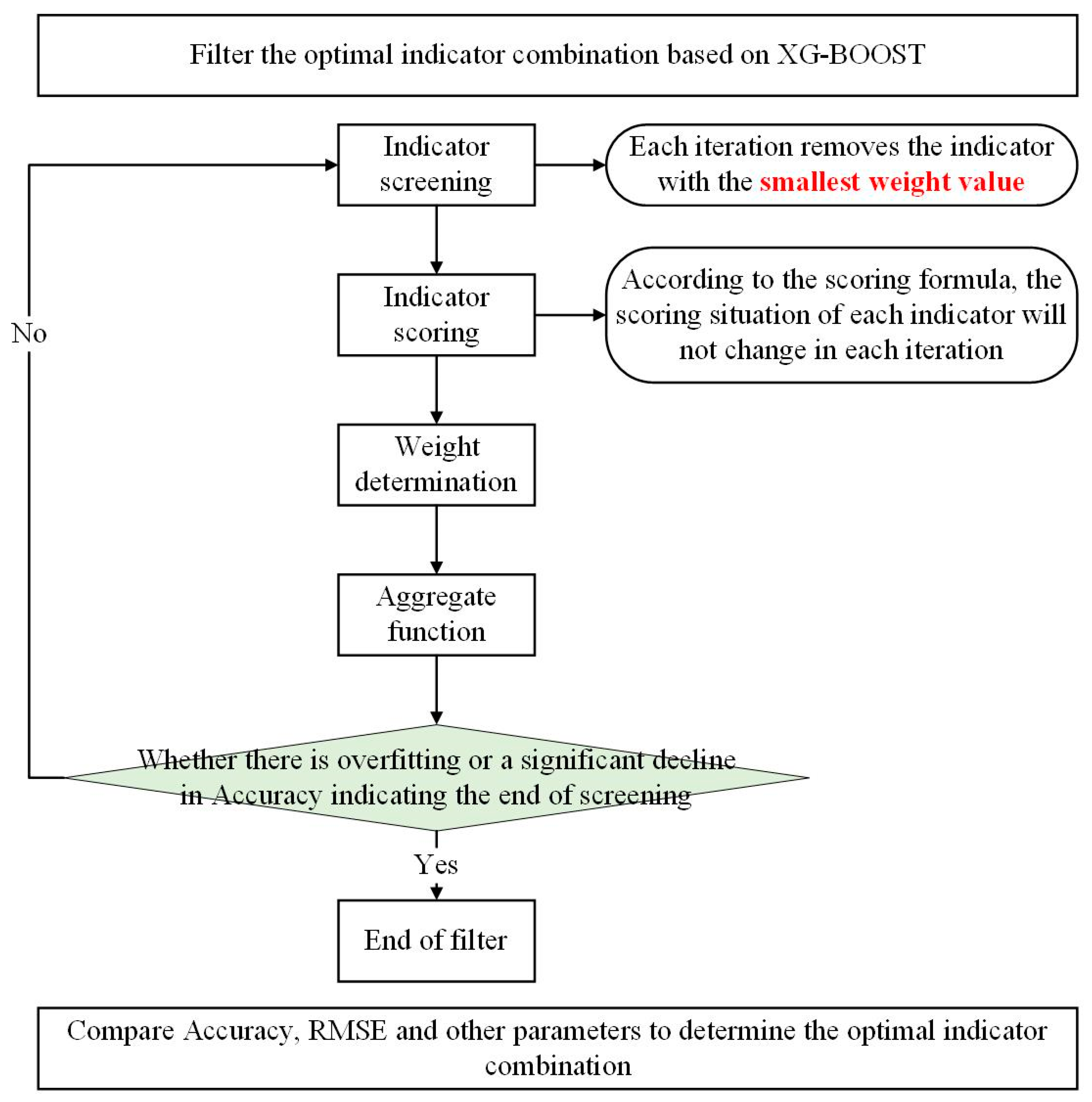
2.5. Screening of the Optimal Set of Water Quality Indicators

When utilizing the WQI evaluation method for water quality assessment, it contains four steps: indicator screening, sub-indicator scoring, assignment, and aggregation. Among these, the processes of indicator screening and assignment greatly influence the results of the water quality evaluation. By using XG-BOOST to determine the weights of the water quality indicators, we improved the process that has traditionally relied on expert knowledge and experience, which has often led to a lack of objectivity in the evaluation results. The following research focuses on the impact of indicator selection on the evaluation results.
In this study, the screening of indicators was carried out so as to select the optimal water quality indicator dataset, and the specific process was as follows (Figure 2):
(1)
Input the concentration data of the ten indicators and water quality status into XG-BOOST to obtain the weight values for each indicator, as well as evaluation metrics such as RMSE, R2, and accuracy under the ten-indicator scenario. Additionally, other standard metrics like the AUC-ROC curve will be obtained.
(2)
Remove the indicator with the smallest weight and determine whether its removal affects the water quality status. If there is a change in water quality status, modify the input water quality status for the corresponding monitoring point, and recalculate using XG-BOOST.
(3)
Continue this process until clear signs of overfitting or other issues arise, at which point the screening ends.
(4)
Compare the model evaluation metrics after each round of screening to comprehensively select the optimal indicator dataset.
(5)
Create spatial distribution maps of the water quality index for each dataset, and analyze the impact of indicator selection on water quality assessment.

3. Results

The following subsections include a description of the results of the experiment and their interpretation, which were the basis for the conclusions drawn.

3.1. WQI Water Quality Analysis

Concentration values of ten water quality indicators at 246 monitoring sites and water quality status (see Table S1 in the Supplementary Materials) were input into the XG-BOOST model, and results such as indicator weights were obtained through training and testing.

3.1.1. Sub-Indicator Scoring

According to the calculation formula for sub-indicators, the scores for ten water quality indicators at 246 monitoring points were computed, and the results are presented in Figure 3. From Formula (1), we can see that when a sub-indicator score is less than 100, it indicates that the concentration of that indicator at the point is below the maximum allowable value specified in the standard, meaning that the concentration is within acceptable limits. Conversely, when the sub-indicator score exceeds 100, it signifies that the concentration of that indicator at the point is above the maximum allowable value, and the more the score exceeds 100, the more severe the excess concentration.
From Figure 3, we can observe that none of the 246 monitoring points showed exceedances for Ag, while SO exceeded allowable values at only a few points. In contrast, Zn, Se, and Pb had significantly more exceedance points compared to the other indicators, with some points for NO and Zn having the highest exceedance multiples among the indicators. Specifically, NO exhibited exceedances as high as 200 times the allowable value at certain points.

3.1.2. Indicator Assignment

After training and testing with XG-BOOST, the relative importance of the ten water quality indicators on the water quality status can be calculated, and these values are used as the weights for each indicator. The specific weighting results are shown in Table 3. From the results, it can be observed that, among the ten water quality indicators, Ag has the smallest weight, indicating that it has the least influence on the water quality status.
The evaluation parameters for the learning performance of the XG-BOOST model are accuracy = 92%, R2 = 0.3355, and RMSE = 0.2828. This indicates a relatively high accuracy for this learning process, suggesting that the predicted water quality status closely matches the actual values based on the learned relationships between the independent and dependent variables. However, the low correlation (R2 value) implies poor model fitting. The small RMSE value indicates a low margin of error. Additionally, the AUC-ROC curve (Figure 4a) and the LOSS curve (Figure 4b) are shown in Figure 4. From the figures, it can be seen that the AUC value is 0.91, indicating relatively accurate predictions, correctly predicting “1” as “1” and “0” as “0”. The slight fluctuations observed during the decline in the LOSS curve suggest that the training process may be somewhat unstable.

3.1.3. Aggregation

After multiplying the indicator weights by the indicator scores for each monitoring point and summing them, the water quality index for that point was obtained. The calculation results are shown in the Supplementary Materials. Using the Geographic Information System (GIS), the water quality indices for each point were imported, and spatial interpolation was performed. Before spatial interpolation, data analysis was conducted using the exploratory data analysis tools in the geostatistical analysis module of the GIS. The exploratory data analysis involved two tools: histogram analysis, and normal QQPlot distribution. Histogram analysis can be used to check data distribution and identify outliers, while the normal QQPlot distribution is used to assess the normality of the data. The closer the distribution is to a straight line, the more the data follow a normal distribution. In the exploratory data analysis, a log transformation was applied to the data. After taking the logarithm of the water quality index data, it showed a clear normal distribution (see Figure 5c). Moreover, through a comparison of Figure 5d,e, it is evident that the data fit better after the log transformation. For data that exhibit normal characteristics, kriging interpolation is generally used for spatial interpolation. In this study, ordinary kriging interpolation was employed. After interpolating the water quality index data, a classification was performed, and the results are shown in Figure 5a.
Figure 5a shows that the water quality of the study area was assessed by ten water quality indicators, and the water quality of the area was mostly “GOOD” and “POOR”. The proportion of the area under “GOOD” and “POOR” was 48.7%, while the proportion of the area under “POOR” was 31.6%. The area with “UNFIT” water quality was mainly distributed in the east–central part of the study area, which is located in part of the Changji Hui Autonomous Prefecture, and the water quality in the western part of the study area was relatively better than that in the eastern part of the study area, while the area with “EXCELLENT” water quality was mainly distributed in the southern part of the study area.

3.2. Optimal Dataset Screening

After iteration, each time the indicator with the smallest weight is eliminated, check whether the water quality status changes, and synchronize the model input data for modification. Each iteration can obtain a set of calculation results containing the weights, evaluation criteria parameters, evaluation criteria graph lines, and the corresponding water quality index. After the ninth iteration, eliminating eight indicators, the model training shows an obvious overfitting phenomenon, and the iteration is over. Each iteration of the weighting results is shown in Figure 6.
From Figure 6, we can observe that, after the first iteration, Ag had the smallest weight and was thus removed first. As shown in the original dataset (Supplementary Materials, Table S1), Ag does not exceed the allowable limit at any monitoring point, so its removal does not affect the “water quality status” input for the next iteration. After removing Ag, the second iteration revealed that Al had the smallest weight, so it was removed next. The original dataset (Supplementary Materials, Table S1) shows that Al exceeds the limit at 17 points, with only Al exceeding the limit at the point whose serial number is 5. Therefore, its removal changes the water quality status input from 1 to 0 for this point. Other monitoring points have other indicators exceeding the limits, so their water quality status remains unaffected.
After removing Ag and Al, SO had the smallest weight and was thus removed in the third iteration. According to the original dataset (Supplementary Materials, Table S1), SO exceeds the limit at three points, but all three also have other indicators exceeding the limits, so removing SO does not affect the “water quality status” input for subsequent iterations. After removing Ag, Al, and SO, Fe had the smallest weight and was removed in the fourth iteration. The original dataset (Supplementary Materials, Table S1) indicates that Fe exceeds the limit at 30 monitoring points, with three points—serial numbers 2, 6, and 229—only having Fe exceed the limit. Thus, removing Fe changes their water quality status from 1 to 0, while the other points have other indicators exceeding the limits, so their water quality status remains unchanged.
After removing the Ag, Al, SO, and Fe indicators, it can be observed that the weight value of F was the smallest. Therefore, in the fifth step, the F indicator was removed. According to the original dataset (Supplementary Materials, Table S1), there are 27 monitoring points where F exceeds the standard. Among them, at monitoring point 246, only the F indicator exceeded the standard. Thus, the removal of the F indicator impacted the water quality status, changing it from 1 to 0. For other points, since there were other indicators exceeding the standard, the water quality status remained unchanged.
After removing the Ag, Al, SO, Fe, and F indicators, it was noted that the weight value of Zn was the smallest. Therefore, in the sixth step, the Zn indicator was removed. According to the original dataset (Supplementary Materials, Table S1), there are 83 monitoring points where Zn exceeds the standard. Among these, a total of 25 monitoring points had only the Zn indicator exceeding the standard. Therefore, the removal of the Zn indicator affected the water quality status, changing it from 1 to 0. For the other points, since there were other indicators exceeding the standard, the water quality status remained unchanged.
After removing Ag, Al, SO, Fe, F, and Zn, Cl had the smallest weight and was removed in the seventh iteration. The original dataset (Supplementary Materials, Table S1) shows that Cl exceeds the limit at 57 points, with 19 points having only Cl exceed the limit. Thus, removing Cl changes their water quality status from 1 to 0, while the other points have other indicators exceeding the limits, so their water quality status remains unchanged. After removing Ag, Al, SO, Fe, F, Zn, and Cl, NO had the smallest weight and was removed in the eighth iteration. According to the original dataset (Supplementary Materials, Table S1), NO exceeds the limit at 57 points, with 32 points having only NO exceed the limit. Thus, removing NO changes their water quality status from 1 to 0, while the other points have other indicators exceeding the limits, so their water quality status remains unchanged.
After removing Ag, Al, SO, Fe, F, Zn, Cl, and NO, the remaining two indicators resulted in an accuracy of 100%, an RMSE of 0, and an R2 of 1.0. Based on other evaluation curves, we deduced that this phenomenon might be caused by excessive indicator removal, leading to a reduced dataset and the inability of the training group to properly learn the relationship between dependent and independent variables, resulting in overfitting. Thus, indicator selection ended at this point, and the next step involved comparing evaluation criteria to select the optimal indicator set.

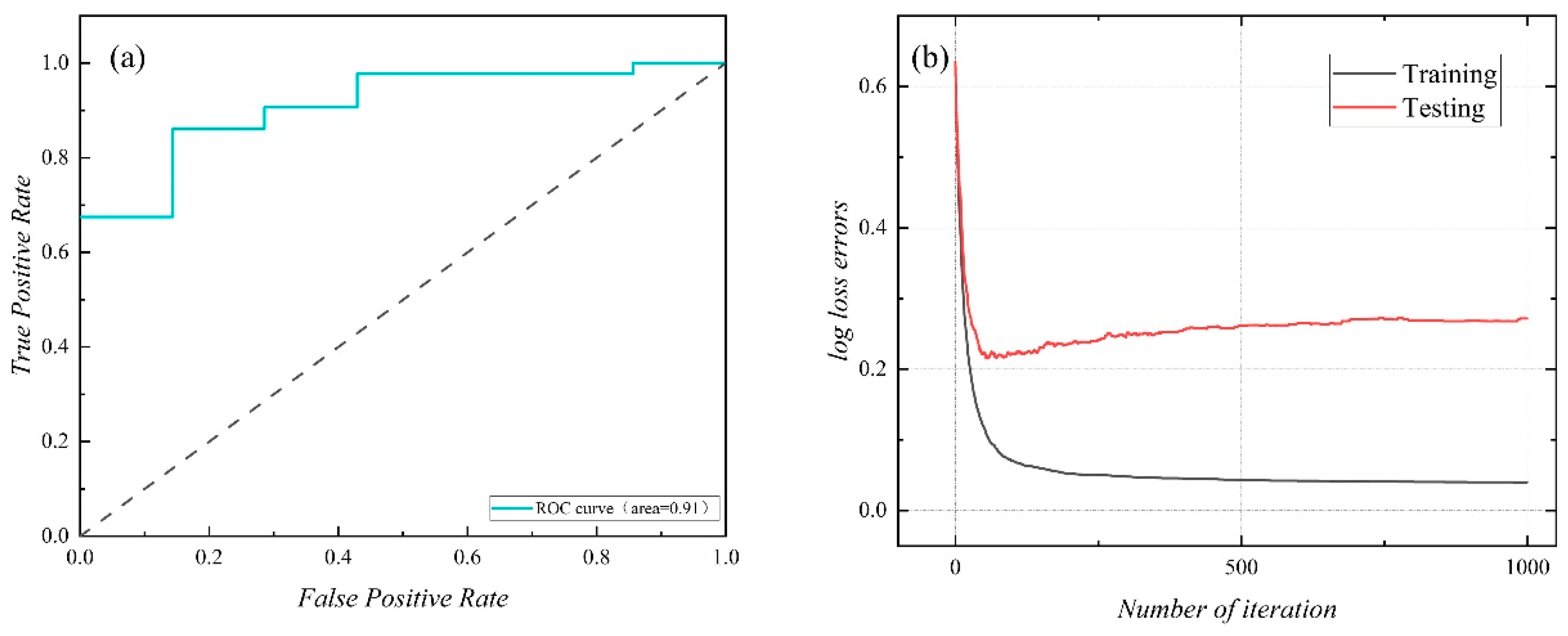
3.2.1. Evaluation Criteria

After the elimination of water quality indicators by XG-BOOST, the evaluation criteria, including three evaluation parameters (accuracy, RMSE, and R2) and two evaluation graph lines (AUC-ROC and LOSS), were used to comprehensively screen the optimal water quality indicator dataset so that the XG-BOOST model predicted the best effect and model performance.
  • Evaluation parameters:
The evaluation parameters obtained from each data iteration are shown in Table 4 and Figure 7, where accuracy is presented as a decimal rather than a percentage for ease of presentation.
As shown in Table 4, there is no clear trend in the changes in various evaluation parameters as the number of indicators decreases, indicating that the model’s performance does not exhibit a simple linear change with the variation in the number of indicators. Additionally, aside from the potential overfitting scenario in the final iteration, it is noteworthy that, during the sixth iteration, after removing five water quality indicators—Ag, Al, SO, Fe, and F—the accuracy reached a maximum of 98%, RMSE reached a minimum of 0.1414, and R2 reached a maximum of 0.9081. This means that, at this point, the model achieved the highest prediction accuracy, the smallest error, and the best fitting performance.
2.
AUC-ROC curve:
The AUC values obtained from each data iteration are shown in Table 4, and the AUC-ROC curves are displayed in Figure 8. First, in terms of trends, the model’s discriminative ability does not show a simple upward or downward trend as the number of indicators decreases. Second, in terms of values, the AUC values for all nine iterations are greater than 0.5, indicating that XG-BOOST maintained a discriminative effect in these training sessions. The best discriminative effect was achieved in the eighth iteration, after removing seven water quality indicators, with an AUC of 0.98. Additionally, the fourth iteration (after removing three indicators) and the sixth iteration (after removing five indicators) also showed relatively good discriminative effects, with an AUC of 0.97.
3.
LOSS curve:
The LOSS curves obtained from each data iteration are shown in Figure 9. From the figure, it can be seen that, on the one hand, the training effectiveness of the model does not show a simple improvement or deterioration trend as the number of indicators decreases. At the early stages of training, the LOSS values generally decrease as the number of training iterations increases, indicating that the model is in a learning state. In the second iteration, however, the LOSS value for the validation set starts to rise after the initial training phase, possibly due to overfitting. In the ninth iteration, the LOSS value for the validation set is even lower than that of the training set, suggesting a possible occurrence of overfitting, likely due to the excessive removal of water quality indicators and the reduced amount of data. On the other hand, during the sixth iteration, after removing five water quality indicators, the LOSS curve continues to decrease, with relatively minor fluctuations compared to other iterations. This indicates that, based solely on training loss, the model achieved its best performance in the sixth iteration, demonstrating good training effectiveness.

3.2.2. Comprehensive Evaluation

Based on a comprehensive assessment using the three evaluation parameters—accuracy, RMSE, and R2—along with the AUC-ROC and LOSS curves, the results indicate that the optimal indicator dataset for maximizing the performance of the XG-BOOST model was achieved in the sixth iteration, after removing Ag, Al, SO, Fe, and F. The remaining dataset included five water quality indicators: Cl, NO, Pb, Se, and Zn. This conclusion was drawn because, in the sixth iteration, the accuracy reached a maximum of 98%, the RMSE reached a minimum of 0.1414, and R2 reached a maximum of 0.9081, indicating the highest prediction accuracy, the smallest error, and the best fitting performance. Although the AUC value was 0.97, slightly lower than the highest value of 0.98 from the eighth iteration, the difference was minimal. Additionally, during the sixth iteration, the LOSS curve showed a continuous decline, with less fluctuation compared to other iterations, indicating optimal model performance and good training effectiveness in terms of training loss. This comprehensive judgment leads to the final result.

3.3. Comparative Results of Water Quality Analysis

After each data iteration, the water quality index distribution map of the response dataset can also be obtained according to the different values of the indicator weights, and the results of the analysis are shown in Figure 10.
From the water quality index distribution map, it can be seen that, if the indicator dataset from the sixth iteration is taken as the optimal dataset, the model achieves its best training performance at this stage. The water quality interpolation results for the other iterations are slightly more favorable compared to the sixth iteration. During the sixth iteration, the proportion of the area classified as having “UNFIT” water quality was the highest, and the area classified as “VERY POOR” was also at its highest proportion. In contrast, by the ninth iteration, the water quality was only classified as “EXCELLENT” and “GOOD”, further indicating a potential occurrence of overfitting, leading to overly optimistic water quality results.

4. Discussion

This study improved the traditional WQI water quality evaluation method, which heavily relied on expert knowledge and experience to determine the weight of water quality indicators, thus leading to a lack of objectivity in the evaluation results. After the first iteration of the original dataset, it was found that accuracy = 92%, R2 = 0.3355, and RMSE = 0.2828, indicating that the accuracy of this learning process is relatively high. That is, the model’s predicted water quality state is close to the true values, with a small discrepancy. However, the correlation is low, suggesting that the model’s fitting effect is not ideal. The small RMSE value indicates that the error is minimal. Although the evaluation standards did not all reach their optimal state after the first iteration, during the selection of the optimal indicator dataset, there were instances where all evaluation standards performed well. This suggests that the XG-BOOST model can effectively learn the relationships between various water quality indicators and the water quality state, and it can make predictions with relatively high accuracy. However, the learning and prediction results are related to the selection of the water quality indicators. In other words, the XG-BOOST model improves the traditional WQI water quality evaluation method and is applicable to the water quality indicator dataset of the study area, enhancing the objectivity and scientific nature of the evaluation results.
Secondly, the results of the groundwater quality study in certain areas of the Manas River Basin in Xinjiang show that the regions where water quality is classified as “UNFIT” are mainly located in the central and eastern parts of the study area, particularly in some areas of the Changji Hui Autonomous Prefecture. Relatively speaking, the western part of the study area has better water quality compared to the eastern part. The areas with “EXCELLENT” water quality are mainly found in the southern part of the study area. Groundwater in the regions classified as “EXCELLENT” and “GOOD” meets the national drinking water standards and should primarily focus on protection to prevent source and process pollution from deteriorating the water quality. Groundwater in the areas with “POOR”, “VERY POOR”, and “UNFIT” water quality does not meet the national drinking water standards and is unsuitable for consumption. Therefore, groundwater in these areas should focus on remediation, adopting measures such as reducing pollution sources to optimize the regional water quality and prevent further deterioration. These findings are expected to be applied to the actual protection and management of local groundwater, providing practical guidance for the evaluation and management of the groundwater environment in the area, and contributing to the sustainable development of local groundwater resources. Additionally, the use of the XG-BOOST model to improve the traditional WQI water quality evaluation method offers a new approach and reference for groundwater quality evaluation in other regions, leading to a deeper development of machine learning methods in groundwater quality assessment.
In the WQI evaluation process, in addition to improving the weighting process through the XG-BOOST model, the impact of indicator selection on the WQI evaluation results was also studied. By combining the XG-BOOST model with the WQI method, the optimal indicator dataset that achieved the best model performance was identified from the ten collected indicators (Cl, NO, Pb, Se, and Zn). This dataset resulted in a maximum accuracy of 98%, a minimum RMSE of 0.1414, and a maximum R2 of 0.9081. In other words, at this point, the model’s prediction accuracy reached its highest level, with the smallest error and the best fitting performance. The AUC was 0.97, and during the sixth iteration, the LOSS curve continued to decline, with less noticeable oscillation compared to other iterations, indicating optimal model performance in terms of training loss and good training results. Additionally, a comparison was made of the water quality classification results aggregated from various indicator datasets during the selection process. It was found that, based on this study’s dataset, the other indicator datasets showed less favorable water quality evaluation results compared to the optimal indicator dataset. However, there are also issues that need further study and discussion:
  • The results of this analysis are based on data from ten water quality indicators and 246 monitoring points. It remains uncertain whether selecting an optimal indicator dataset based on more water quality indicators in the region would yield the same results as this study. However, regardless of whether the same results can be obtained, the method of improving the traditional WQI with XG-BOOST has been proven effective for assessing groundwater quality. In the future, this method can be applied to more datasets to verify whether the results are consistent.
  • The selection of the optimal water quality dataset in this study was primarily based on evaluation criteria to determine the final results. Therefore, the causes of any anomalies, such as significant fluctuations in the LOSS curve during each iteration of the selection process, were not thoroughly analyzed, and only possible causes were speculated. Future research could focus on how to effectively analyze and address model overfitting when using XG-BOOST to improve the traditional WQI method for water quality assessment.
  • In this study, spatial interpolation was used in the process of investigating the spatial distribution of water quality indices using GISs. However, only an appropriate spatial interpolation method was selected based on the characteristics of the data distribution, without an in-depth exploration of how different spatial interpolation methods impact the results of the spatial distribution of water quality indices. Additionally, this study did not investigate how to choose different interpolation methods based on factors such as the amount of data and the characteristics of their distribution. This could be explored as a research topic in the future for further analysis and validation.
  • The main focus of this study is on analyzing the current status of regional groundwater quality. Equally important as the current situation are the potential factors that contribute to the deterioration of water quality. Changes in these factors, such as land-use type, climate change, and changes in pollution sources, will affect the future state of groundwater quality. This could be explored as a future research direction, focusing on predicting groundwater quality under changing conditions.

Supplementary Materials

The following supporting information can be downloaded at https://www.mdpi.com/article/10.3390/su162410991/s1: Table S1: Data table of concentration of ten water quality indicators at 246 monitoring points. Table S2: Water quality index calculation results. Table S3: The optimal indicator set. Figure S1: Indicator weights and spatial distribution of water quality levels in the optimal indicator dataset.

Author Contributions

Conceptualization, J.L. and Q.C.; data curation, W.Y. (Wenchao Yuan); formal analysis, J.L.; methodology, W.Y. (Weifeng Yue); project administration, D.Z.; software, W.Y. (Wenchao Yuan); supervision, W.Y. (Weifeng Yue); validation, J.L., Q.C. and W.Y. (Weifeng Yue); visualization, J.L.; writing—original draft, J.L.; writing—review and editing, J.L. All authors have read and agreed to the published version of the manuscript.

Funding

This research was funded by Research on Key Technologies of Ecological Security Pattern Construction and Risk Control in Luanhe River Basin, grant number 21373904D.

Institutional Review Board Statement

Not applicable.

Informed Consent Statement

Not applicable.

Data Availability Statement

The original contributions presented in this study are included in the article/Supplementary Materials; further inquiries can be directed to the corresponding authors.

Acknowledgments

The authors would like to give thanks for the provision of data for this research within the projects “Research on Key Technologies of Ecological Security Pattern Construction and Risk Control in Luanhe River Basin”.

Conflicts of Interest

The authors declare no conflicts of interest. The funders had no role in the design of the study; in the collection, analyses, or interpretation of data; in the writing of the manuscript; or in the decision to publish the results.

References

  1. Li, P.-Y.; Hui, Q.; Wu, J.H. Application of Set Pair Analysis Method Based on Entropy Weight in Groundwater Quality Assessment—A Case Study in Dongsheng City, Northwest China. J. Chem. 2010, 8, 851–858. [Google Scholar] [CrossRef]
  2. Li, P.; Wu, J.; Qian, H. Groundwater quality assessment based on rough sets attribute reduction and TOPSIS method in a semi-arid area, China. Environ. Monit. Assess. 2011, 184, 4841–4854. [Google Scholar] [CrossRef]
  3. Liyan, Y.; Xiaoyan, L. Application of Single-Factor Evaluation Method and Canadian Water Quality Index Method in Water Source Quality Evaluation—Taking the “Thousand Tons for Ten Thousand People” Drinking Water Source of Jiuquan City as an Example. China Resour. Compr. Util. 2021, 39, 48–51. [Google Scholar]
  4. Weina, G.; Lin, L.; Qin, H.; Tao, L. Exploration and Application of Single-Factor Index Method in Drinking Water Quality Evaluation. Water Supply Drain. 2016, 52, 150–154. [Google Scholar]
  5. Su, K.; Wang, Q.; Li, L.; Cao, R.; Xi, Y.; Li, G. Water quality assessment based on Nemerow pollution index method: A case study of Heilongtan reservoir in central Sichuan province, China. PLoS ONE 2022, 17, e0273305. [Google Scholar] [CrossRef] [PubMed]
  6. Zhang, Q.; Feng, M.; Hao, X. Application of Nemerow Index Method and Integrated Water Quality Index Method in Water Quality Assessment of Zhangze Reservoir. IOP Conf. Ser. Earth Environ. Sci. 2018, 128, 012160. [Google Scholar] [CrossRef]
  7. Zhang, X.F.; Xiao, C.L.; Li, Y.Q.; Song, D.F. Water Environmental Quality Assessment and Protection Strategies of the Xinlicheng Reservoir, China. Appl. Mech. Mater. 2014, 501–504, 1863–1867. [Google Scholar] [CrossRef]
  8. Zhao, K. Set Pair Analysis and Its Preliminary Application. Exploration of Nature 1994. Available online: https://kns.cnki.net/KCMS/detail/detail.aspx?dbcode=CJFN&dbname=CJFDN7904&filename=DZRT401.011 (accessed on 11 February 2024).
  9. Wang, H.L.; Zhang, J.F.; Lei, H.Y.; Lv, L.L.; Fu, T.T.; Li, H.F. Evaluation of Groundwater Resource Utilization in Mining Subsidence Areas in Henan Based on AHP-Set Pair Analysis Method. People’s Yellow River 2024, 46, 72–77+89. [Google Scholar]
  10. Fan, Z.J.; Wei, X.; Li, J.W.; Zhou, Y.L. Research Progress on Groundwater Drinking Water and Irrigation Water Quality Evaluation Methods. Groundwater 2022, 44, 10–15. [Google Scholar]
  11. Piyathilake, I.D.U.H.; Ranaweera, L.V.; Udayakumara, E.P.N.; Gunatilake, S.K.; Dissanayake, C.B. Assessing groundwater quality using the Water Quality Index (WQI) and GIS in the Uva Province, Sri Lanka. Appl. Water Sci. 2022, 12, 72. [Google Scholar] [CrossRef]
  12. Ababakr, F.A. Spatio-temporal variations of groundwater quality index using geostatistical methods and GIS. Appl. Water Sci. 2023, 13, 206. [Google Scholar] [CrossRef]
  13. Mahmud, A. Assessment of groundwater quality in Khulna city of Bangladesh in terms of water quality index for drinking purpose. Appl. Water Sci. 2020, 10, 1–14. [Google Scholar] [CrossRef]
  14. Rahman, M.M. Investigation of groundwater and its seasonal variation in a rural region in Natore, Bangladesh. Heliyon 2024, 10, e32991. [Google Scholar] [CrossRef]
  15. Gabr, M.E. Groundwater quality evaluation for drinking and irrigation uses in Dayrout city Upper Egypt. Ain Shams Eng. J. 2020, 12, 327–340. [Google Scholar] [CrossRef]
  16. Krishan, G. Integrated approach for the investigation of groundwater quality through hydrochemistry and water quality index (WQI). Urban Clim. 2022, 47, 101383. [Google Scholar] [CrossRef]
  17. Uddin, M.G.; Rana, M.M.S.P.; Diganta, M.T.M.; Bamal, A.; Sajib, A.M.; Abioui, M.; Shaibur, M.R.; Ashekuzzaman, S.; Nikoo, M.R.; Rahman, A.; et al. Enhancing groundwater quality assessment in coastal area: A hybrid modeling approach. Heliyon 2024, 10, e33082. [Google Scholar] [CrossRef] [PubMed]
  18. Seifi, A.; Dehghani, M.; Singh, V.P. Uncertainty analysis of water quality index (WQI) for groundwater quality evaluation_ Application of Monte-Carlo method for weight allocation. Ecol. Indic. 2020, 117, 106653. [Google Scholar] [CrossRef]
  19. El-Magd, S.A.A. Integrated machine learning–based model and WQI for groundwater quality assessment: ML, geospatial, and hydro-index approaches. Environ. Sci. Pollut. Res. 2023, 30, 53862. [Google Scholar]
  20. Huang, Y.; Wang, C.; Wang, Y.; Lyu, G.; Lin, S.; Liu, W.; Niu, H.; Hu, Q. Application of machine learning models in groundwater quality assessment and prediction: Progress and challenges. Front. Environ. Sci. Eng. 2024, 18, 29. [Google Scholar] [CrossRef]
  21. Zegaar, A.; Ounoki, S.; Telli, A. Machine Learning for Groundwater Quality Classification: A Step Towards Economic and Sustainable Groundwater Quality Assessment Process. Water Resour. Manag. 2024, 38, 621–637. [Google Scholar] [CrossRef]
  22. Singha, S.S.; Singha, S.; Pasupuleti, S.; Venkatesh, A.S. Knowledge-driven and machine learning decision tree-based approach for assessment of geospatial variation of groundwater quality around coal mining regions, Korba district, Central India. Environ. Earth Sci. 2022, 81, 36. [Google Scholar] [CrossRef]
  23. Wang, X.; Tian, Y.; Liu, C. Assessment of groundwater quality in a highly urbanized coastal city using water quality index model and bayesian model averaging. Front. Environ. Sci. 2023, 11, 1086300. [Google Scholar] [CrossRef]
  24. Vijay, S. Prediction of Water Quality Index in Drinking Water Distribution System Using Activation Functions Based Ann. Water Resour. Manag. 2021, 35, 535–553. [Google Scholar] [CrossRef]
  25. Gibrilla, A.; Bam, E.K.P.; Adomako, D.; Ganyaglo, S.; Osae, S.; Akiti, T.T.; Kebede, S.; Achoribo, E.; Ahialey, E.; Ayanu, G.; et al. Application of Water Quality Index (WQI) and Multivariate Analysis for Groundwater Quality Assessment of the Birimian and Cape Coast Granitoid Complex: Densu River Basin of Ghana. Water Qual. Expo. Health 2011, 3, 63–78. [Google Scholar] [CrossRef]
  26. Kang, W.H.; Zhou, Y.Z.; Lei, M.; Han, S.B.; Zhou, J.L. Distribution and Co-Enrichment Mechanism of Arsenic, Fluoride, and Iodine in Groundwater in the Manas River Basin, Xinjiang. China Environ. Sci. 2024, 44, 3832–3842. [Google Scholar]
  27. Kang, W.; Zhou, Y.; Zhou, J.; Jiang, F.; Han, S.; Remy; Liu, J. Distribution Characteristics, Source Analysis, and Health Risk Assessment of Inorganic Components in Groundwater in the Plain Area of the Manas River Basin, Xinjiang. Environ. Sci. 2024, 1–16. [Google Scholar] [CrossRef]
  28. Krishnamoorthy, N.; Thirumalai, R.; Sundar, M.L.; Anusuya, M.; Kumar, P.M.; Hemalatha, E.; Prasad, M.M.; Munjal, N. Assessment of underground water quality and water quality index across the Noyyal River basin of Tirupur District in South India. Urban Clim. 2023, 49, 101436. [Google Scholar] [CrossRef]
  29. GB 5749-2022; Standards for Drinking Water Quality. Jingtai County People’s Government: Baiyin, China, 2022. Available online: https://www.jingtai.gov.cn/zfxxgk/bmhxzxxgk/xzfzcbmzsjgml/xwsjkj/fdzdgknr/jzsshyysszjc/art/2024/art_927619b8e82b48689300d36232d739c1.html (accessed on 1 December 2024).
  30. Uddin, M.G.; Nash, S.; Rahman, A.; Olbert, A.I. A comprehensive method for improvement of water quality index (WQI) models for coastal water quality assessment. Water Res. 2022, 219, 118532. [Google Scholar] [CrossRef] [PubMed]
  31. Liu, Q.; Wang, Z.; Xu, H.; Lian, W.; Chen, Y. PM2.5 Concentration Inversion Based on Particle Swarm Optimized XG-Boost Model. Environ. Sci. 2024, 49, 1–16. [Google Scholar] [CrossRef]
Figure 1. Map of the study area: (a) Location map of the study area in China. (b) Location map of the study area in Xinjiang Province, and elevation images of Xinjiang Province. (c) Images of the study area, and distribution of monitoring site locations in the study area.
Sustainability 16 10991 g001
Figure 2. Flowchart for screening the optimal water quality indicator dataset.
Sustainability 16 10991 g002
Figure 3. Plots of the results: (aj) Scatterplots of the scores for the sub-indicators F, Cl, NO, SO, Ag, Al, Fe, Pb, Se, and Zn, respectively. The color indicator bar on the right side of the figure represents the range of different sub-indicator scores. When the sub-indicator score is less than 100, the scatter points are green, indicating that the concentration of the sub-indicator at this monitoring point has not exceeded the maximum allowable standard value. When the sub-indicator score is greater than 100 but less than 200, the scatter points are blue; when the score is greater than 200 but less than 500, the scatter points are yellow; when the score is greater than 500 but less than 1000, the scatter points are orange; and when the score is greater than 1000, the scatter points are red. That is, except for the green scatter points, all other colors represent an exceedance of the standard, and the higher the color indicator bar, the more severe the exceedance.
Sustainability 16 10991 g003
Figure 4. (a) AUC-ROC curve; (b) LOSS curve.
Sustainability 16 10991 g004
Figure 5. Exploratory analysis and spatial distribution map of water quality index: (a) Distribution of water quality in the study area. (b) Histogram of data exploration before subjecting the water quality index data to log computation. (c) Histogram of data exploration after subjecting the water quality index data to log computation. (d) Fitted plot of data exploration before subjecting the water quality index data to log computation. (e) Fitted plot of data exploration after subjecting the water quality index data to log computation.
Sustainability 16 10991 g005
Figure 6. Iterative water quality indicator weight plots for XG-BOOST run data: (ai) the weight values of each indicator obtained from model training when 0–8 water quality indicators are removed, respectively. The red letter in each figure represents the weight value of the water quality indicator with the least weight in the results of this data iteration, that is, the indicator will be eliminated before the next data iteration.
Sustainability 16 10991 g006
Figure 7. Spider web diagram of evaluation parameters.
Sustainability 16 10991 g007
Figure 8. AUC-ROC curves obtained from each iteration of the data. Panels (ai) represent the results of the first through ninth iterations, respectively. The first iteration refers to the XG-BOOST algorithm applied to the original dataset. The second iteration refers to the calculation performed after removing the indicator Ag, which had the lowest weight in the first iteration. The third iteration refers to the calculation performed after removing the indicator Al, which had the lowest weight in the second iteration, resulting in a dataset with two indicators removed. This process continued as follows: the fourth iteration refers to the calculation performed after removing the indicators Ag, Al, and SO; the fifth iteration refers to the calculation after removing Ag, Al, SO, and Fe; the sixth iteration refers to the calculation after removing Ag, Al, SO, Fe, and F; the seventh iteration refers to the calculation after removing Ag, Al, SO, Fe, F, and Zn; the eighth iteration refers to the calculation after removing Ag, Al, SO, Fe, F, Zn, and Cl; and the ninth iteration refers to the calculation after removing Ag, Al, SO, Fe, F, Zn, Cl, and NO. The area value in the bottom right corner of each chart represents the AUC value, and the dashed line in the figure indicates AUC = 0.5.
Sustainability 16 10991 g008
Figure 9. Training LOSS plots from (ai) represent the results of the plots obtained from the first through ninth iterations of data, respectively. The first iteration refers to the calculation using the XG-BOOST algorithm on the original dataset. The second iteration refers to the calculation after removing the indicator Ag, which had the lowest weight in the first iteration. The third iteration refers to the calculation after removing the indicator Al, which had the lowest weight in the second iteration, resulting in a dataset with two indicators removed. This process continued as follows: the fourth iteration refers to the calculation after removing the indicators Ag, Al, and SO; the fifth iteration refers to the calculation after removing Ag, Al, SO, and Fe; the sixth iteration refers to the calculation after removing Ag, Al, SO, Fe, and F; the seventh iteration refers to the calculation after removing Ag, Al, SO, Fe, F, and Zn; the eighth iteration refers to the calculation after removing Ag, Al, SO, Fe, F, Zn, and Cl; and the ninth iteration refers to the calculation after removing Ag, Al, SO, Fe, F, Zn, Cl, and NO.
Sustainability 16 10991 g009
Figure 10. Distribution of water quality indices: (ai) The interpolated plots of water quality indices obtained from the first through ninth iterations of data, respectively. The first iteration refers to the calculation using the XG-BOOST algorithm on the original dataset. The second iteration refers to the calculation after removing the indicator Ag, which had the lowest weight in the first iteration. The third iteration refers to the calculation after removing the indicator Al, which had the lowest weight in the second iteration, resulting in a dataset with two indicators removed. This process continued as follows: the fourth iteration refers to the calculation after removing the indicators Ag, Al, and SO; the fifth iteration refers to the calculation after removing Ag, Al, SO, and Fe; the sixth iteration refers to the calculation after removing Ag, Al, SO, Fe, and F; the seventh iteration refers to the calculation after removing Ag, Al, SO, Fe, F, and Zn; the eighth iteration refers to the calculation after removing Ag, Al, SO, Fe, F, Zn, and Cl; and the ninth iteration refers to the calculation after removing Ag, Al, SO, Fe, F, Zn, Cl, and NO. The rings in the lower left corner of each plot show the percentage of the study area occupied by each water quality class, and their colors are the same as those represented by the water quality classes in the interpolated plots, with blue denoting “EXCELLENT”, green denoting “GOOD”, yellow denoting “POOR”, orange denoting “VERY POOR”, and red denoting “UNFIT”.
Sustainability 16 10991 g010
Table 1. Maximum allowable values for water quality indicator concentrations. Unit: mg/L.
Indicator
Number
Name of IndicatorMaximum Allowable Concentration (Standard)
1F1
2Cl250
3NO10
4SO250
5Ag0.05
6Al0.2
7Fe0.3
8Pb0.01
9Se0.01
10Zn1
Table 2. Water quality index grading scale.
Serial NumberWater Quality Index IntervalRank
1<50EXCELLENT
250–100GOOD
3101–200POOR
4201–300VERY POOR
5>300UNFIT
Table 3. Ten water quality indices’ assignment results table.
Serial NumberName of IndicatorWeighted Value
1F0.08680517
2Cl0.10941678
3NO0.14282118
4SO0.08359309
5Ag0.04725126
6Al0.05445521
7Fe0.06113945
8Pb0.16887292
9Se0.13781276
10Zn0.10783219
Table 4. Table of evaluation parameters.
Exclusion Metrics and Number of IterationsAccuracyRMSER2AUC
(1)0.920.28280.33550.91
Ag (2)0.740.50990.51520.81
Al (3)0.820.42430.06440.93
SO (4)0.960.20.66780.97
Fe (5)0.920.28280.4580.96
F (6)0.980.14140.90810.97
Zn (7)0.90.31620.54040.96
Cl (8)0.960.20.82170.98
NO (9)1011
Note: The first column of the table represents the iteration number and the water quality indicators removed from the dataset during each iteration. For example, “(1)” indicates the first iteration, where the dataset used was the original dataset, with no indicators removed; “Ag (2)” indicates the second iteration, where the water quality indicator Ag was removed because it had the lowest weight in the first iteration; “Al (3)” indicates the third iteration, where the water quality indicator Al was removed because it had the lowest weight in the second iteration. By this point, both Ag and Al had been removed from the dataset. This process continued accordingly for the subsequent iterations.
Disclaimer/Publisher’s Note: The statements, opinions and data contained in all publications are solely those of the individual author(s) and contributor(s) and not of MDPI and/or the editor(s). MDPI and/or the editor(s) disclaim responsibility for any injury to people or property resulting from any ideas, methods, instructions or products referred to in the content.

