Short-Term Output Scenario Generation of Renewable Energy Using Transformer–Wasserstein Generative Adversarial Nets-Gradient Penalty

Abstract

As renewable energy sources are becoming more widely integrated into the modern power system, the uncertainties within this system are becoming increasingly prominent. It is crucial to accurately describe the uncertainties in renewable energy output for the effective planning, scheduling, and control of power systems. For this purpose, the aim of this paper is to introduce a method for generating short-term output scenarios for renewable energy sources based on an improved Wasserstein Generative Adversarial Nets-Gradient Penalty. First, a Deep Neural Network structure inspired by the Transformer algorithm is developed to capture the temporal characteristics of renewable energy outputs. Then, combined with the advantage of the data generation of the Wasserstein Generative Adversarial Nets-Gradient Penalty, the Transformer–Wasserstein Generative Adversarial Nets-Gradient Penalty is proposed to generate short-term renewable energy output scenarios. Finally, experimental validation is conducted on open-source wind and photovoltaic datasets from the U.S. National Renewable Energy Laboratory, where the performance of the proposed model in generating renewable energy output scenarios across various aspects (i.e., individual sample representation, expectation and variance, probability density function, cumulative distribution function, power spectral density, autocorrelation coefficient, and pinball loss) is assessed. The results show that our method outperforms the Wasserstein Generative Adversarial Nets-Gradient Penalty, Variational Autoencoder, Copula function, and Latin Hypercube Sampling models in the abovementioned evaluation indicators, providing a more precise probability distribution representation of realistic short-term renewable energy outputs.

1. Introduction

In order to achieve the goal of sustainable development, industry is attempting to transition from fossil energy to renewable and clean energy markets worldwide [1]. The rapid expansion of renewable energy sources, such as wind and photovoltaic (PV) power, is crucial in achieving the goal of “carbon neutrality”, and they are beneficial in coping with climate change and solving the energy crisis [2]. With the advancement of modern power systems, the integration of wind power and PV into the grid continues to increase. The fluctuating nature and limited predictability of these renewable sources pose significant challenges to the reliability of power system operations and the decision-making process for energy dispatch [3]. Therefore, it is essential to explore modeling techniques that accurately capture the uncertainty associated with wind and PV power.

Currently, studies evaluating the characteristics of renewable energy output mainly focus on the interval and scenario methods. From the perspective of optimizing dispatch decisions, the scenario method is more stable compared to the interval method [4]. Specifically, the scenario method effectively captures the uncertainty inherent in renewable energy and reflects the temporal and spatial dependencies in their generation [5], which is crucial for the economic dispatch of renewable energy [6] and the composition of unit groups [7,8].

For scenario methods, model-driven statistical probability and data-driven artificial intelligence (AI) probability models are the two primary methodologies employed in modeling scenarios for renewable energy output. For reading convenience, a literature review of the different types of methods is summarized in Table 1. The following summarizes the scenario generation methods (which have been employed in some practical applications in the electricity field) of the model-driven statistical probability models: the Markov chain approach, the scenario tree generation technique, and the time-series method [7,9,10,11,12]. Based on the probability distribution of historical data, ref. [7] generated a scenario tree to describe the dependencies between different stages in multi-stage stochastic mixed-integer programming, reflecting the uncertainty in auxiliary service market demand and photovoltaic output, and it was used to formulate a day-ahead unit commitment optimization strategy. Ref. [12] generated source-load scenarios based on the Markov chain method for energy stochastic collaborative optimization. These methodologies presume an uncertainty in wind power and PV outputs as a statistical model with a known probability distribution, and they derive specific parameters of the probability model from the historical data of their scenarios. Then, these probability distribution models are sampled through a sampling method such as Latin Hypercube Sampling (LHS), Monte Carlo Sampling (MCS), and Copula-based Sampling (CS) [13] to generate specific wind power and PV output scenarios. Ref. [14] proposed a sampling model combining LHS and Cholesky decomposition for probabilistic load flow evaluations of the power system. By comparing them with traditional sampling methods, it was proven that this hybrid method is robust and flexible and that it can be effectively applied to other probabilistic problems of power systems such as renewable energy scenario generation. Ref. [15] introduced a Markov Chain Monte Carlo (MCMC) to directly generate a synthetic time series of wind power output. Ref. [16] used the Copula function to describe the spatial and temporal characteristics of wind power output, generated random numbers by sampling, and combined the inverse sampling process utilizing the cumulative distribution function that reflects the characteristics of the prediction error probability to generate wind power output scenarios similar to the actual operating data of Jeju Island. However, due to significant meteorological influences and the complex spatiotemporal coupling between multiple sites, wind power and PV outputs exhibit a strong time-varying nonlinear correlation. Most existing statistical probability models, which consider only a single feature of renewable energy outputs, fail to comprehensively and accurately capture the various correlations and uncertainties in wind power and PV scenarios. Furthermore, these methods either require strong statistical assumptions or detailed empirical data and complex mathematical modeling, making direct application challenging, limiting generalizability, and restricting the diversity of the scenarios generated.

With the rapid advancement of AI algorithms in recent years, the research on data-driven-based probabilistic models for modeling the uncertainty in renewable energy output has gradually garnered widespread attention. Currently, the machine learning algorithms for wind and PV scenario generation predominantly encompass Autoregressive Moving Average Models (ARMAs) [17], Variational Autoencoders (VAEs) [18,19], Normalizing Flows (NFs) [20], and Generative Adversarial Networks (GANs) [21,22,23,24,25]. Generative models such as VAEs, NFs, and GANs are utilized in unsupervised learning to train Deep Neural Networks (DNNs) by learning the pattern of existing data and generating new samples that fit the distribution of the real data. Compared to traditional supervised learning, which struggles with fitting probability distributions and requires large volumes of labeled data, generative models have a pronounced advantage in renewable energy output scenario generation. An improved VAE was utilized in Ref. [18] to characterize the uncertainty of PV outputs and generate its scenarios for the optimal configuration model. Ref. [19] combined the Multi-Collinearity Reduction (MCLR) technique and Conditional VAE (CVAE) to propose a Bayesian generative DNN to generate more accurate source-load random scenarios for the calculation of probabilistic optimal power flow. Ref. [20] proposed NF to generate PV, wind power, and load scenarios. However, VAEs necessitate intricate variational inference to maximize the evidence lower bound, and NFs require strictly invertible design structures [26]. Therefore, the model limitations make VAEs and NFs lack the capability to assess probability distributions accurately, which results in a lower quality of sample generation [27]. The unsupervised architectures of GANs avoid the cumbersome process of manually labeling renewable energy output data or meteorological data, providing superior sample generation performance. Consequently, the current research on renewable energy output scenario generation primarily focuses on the application and enhancement of GANs. Conditional WGANs have been applied to wind power and PV scenario generation in Ref. [21], using training data with weather events or temporal markers within a year to generate scenarios under various conditions. The Davies–Bouldin Index (DBI) was leveraged in Ref. [22] to determine the optimal number of clusters for the renewable energy output scenarios generated by the Wasserstein Generative Adversarial Nets-Gradient Penalty (WGAN-GP) before applying K-Medoids to obtain a set of typical scenarios. The introduction of interpretable latent space into a controllable GAN in Ref. [23] enabled the generation of controllable scenarios encompassing a wide range of statistical properties while being capable of producing new generated scenarios different from known samples. Ref. [24] proposed an improved GAN combined with variational inference (GAN-VI) for renewable energy scenario generation by enhancing traditional GANs with variational inference operation. Ref. [25] employed the principle of maximizing mutual information to improve the VAEGAN model and achieve the generation of controllable scenarios of renewable energy output covering various kinds of output statistical characteristics and with specific preference characteristics. Nevertheless, GANs face challenges in convergence and stability during the training process [28], as well as the mode-collapse issue, which leads to the poor diversity of the generated sample, limited generalization ability, and challenges in covering the entire real data distribution [29]. Moreover, the current GAN-based research predominantly relies on the architecture of the deep Convolutional Neural Network (CNN). CNNs, extracting data features through convolutional kernels, are particularly adept at processing two-dimensional data like images due to their strong capability of capturing local features. However, their convolutional kernels typically have a limited view of a small feature area, which potentially leads to the loss of local details in renewable energy output scenarios. Therefore, it is necessary to explore a method to improve the capabilities of capturing temporal data features and addressing the processing of long-distance dependency relationships among data in the research of scenario generation.

The Transformer is a powerful algorithm that enables the model to weigh the importance of separate parts of the input data relative to each other, thus providing a dynamic method to pay attention to the correlation between information [30]. Its mechanism of action is advantageous in processing time-series data, which has been applied to the prediction of renewable energy output. Ref. [31] proposed a CNN–Long Short-Term Memory (LSTM) Transformer model to extract the spatial and temporal features of the PV output and used Transformer to generate the predicted output results from these features. A data filtering wind and PV output forecasting method based on Transformer was presented in Ref. [32], where the Savitzky–Golay and Local Outlier Factor filters were used to preprocess the data for reducing noise, as well as predicting the renewable output through combining Transformer in the prediction model. Based on the above analysis, this paper proposes a scenario generation approach based on an enhanced WGAN-GP model for short-term renewable energy outputs. Integrating the strengths of the Transformer framework in sequential data feature extraction to construct the neural network architecture of the WGAN-GP generator, the Transformer-WGAN-GP (TWGAN-GP) model is introduced to augment the capability of the generation model in extracting internal features of time-series data. The generator of TWGAN-GP accepts the noise and employs Transformer for embedding its positional features, extracting temporal features, and adjusting data dimensions to generate the output scenarios of renewable energy. Following this, the discriminator distinguishes between the generated and real scenarios. This cycle is iterated for the optimization training of the model until the model is able to attain a precise alignment with the probability distribution of real output scenarios, thereby improving the quality of the generated scenarios.

This paper is structured as follows: Section 2 introduces the proposed TWGAN-GP model; the case studies and results based on an open-source wind power and PV dataset are presented in Section 3; finally, the main conclusions are summarized in Section 4.

Table 1. Literature review on scenario generation.

Generation Model Type	Model		Reference	Shortages in Scenario Generation
Model-Driven Statistical Probability Models	Modeling Methods	Markov Chain Approach	[8,9,10,12]	(1) Insufficient ability to capture various correlations and uncertainties in renewable energy output; (2) Difficulty in direct application and generalizability.
		Scenario Tree Generation Technique	[7]
		Time-Series Method	[11]
	Sampling Methods	LHS	[14]
		MCS	[15]
		CS	[16]
Data-Driven Artificial Intelligence Probability Models	ARMA		[17]	The low fitting ability of the model.
	VAE		[18,19]	Model limitation of intricate variational inference.
	NF		[20]	Model limitation of strictly invertible design structure.
	GANs	Conditional WGAN	[21]	(1) Shortage of generation diversity and generalization to cover the authentic distribution; (2) CNN-based architecture is relatively weak in extraction of temporal properties.
		WGAN-GP	[22]
		Controllable GAN	[23]
		GAN-VI	[24]
		VAEGAN	[25]

Table 1. Literature review on scenario generation.

Generation Model Type	Model		Reference	Shortages in Scenario Generation
Model-Driven Statistical Probability Models	Modeling Methods	Markov Chain Approach	[8,9,10,12]	(1) Insufficient ability to capture various correlations and uncertainties in renewable energy output; (2) Difficulty in direct application and generalizability.
		Scenario Tree Generation Technique	[7]
		Time-Series Method	[11]
	Sampling Methods	LHS	[14]
		MCS	[15]
		CS	[16]
Data-Driven Artificial Intelligence Probability Models	ARMA		[17]	The low fitting ability of the model.
	VAE		[18,19]	Model limitation of intricate variational inference.
	NF		[20]	Model limitation of strictly invertible design structure.
	GANs	Conditional WGAN	[21]	(1) Shortage of generation diversity and generalization to cover the authentic distribution; (2) CNN-based architecture is relatively weak in extraction of temporal properties.
		WGAN-GP	[22]
		Controllable GAN	[23]
		GAN-VI	[24]
		VAEGAN	[25]

2. TWAGN-GP: A New Method for Short-Term Output Scenario Generation of Renewable Energy

A scenario of renewable energy output can be depicted through a definitive output curve. Assuming that $x_t$, where $t=1,2,3,\dots ,T$ are the renewable energy output values over time, have been observed at a certain renewable energy station, then $\mathit{x}=\left\{x_t\right\}$ can be regarded as an output scenario. The real probability distribution of $\mathit{x}$, denoted as $P_{\mathrm{Data}}$, is unknown and challenging to model due to its intricate spatiotemporal correlations.

To accurately describe the characteristics of renewable energy output scenarios, it is imperative to establish an appropriate model to precisely fit the probability distribution of $P_{\mathrm{Data}}$ and obtain an approximate distribution. Subsequently, by sampling from the approximate distribution, scenario generation is accomplished. Therefore, this paper introduces the TWGAN-GP model for the generation of renewable energy output scenarios. 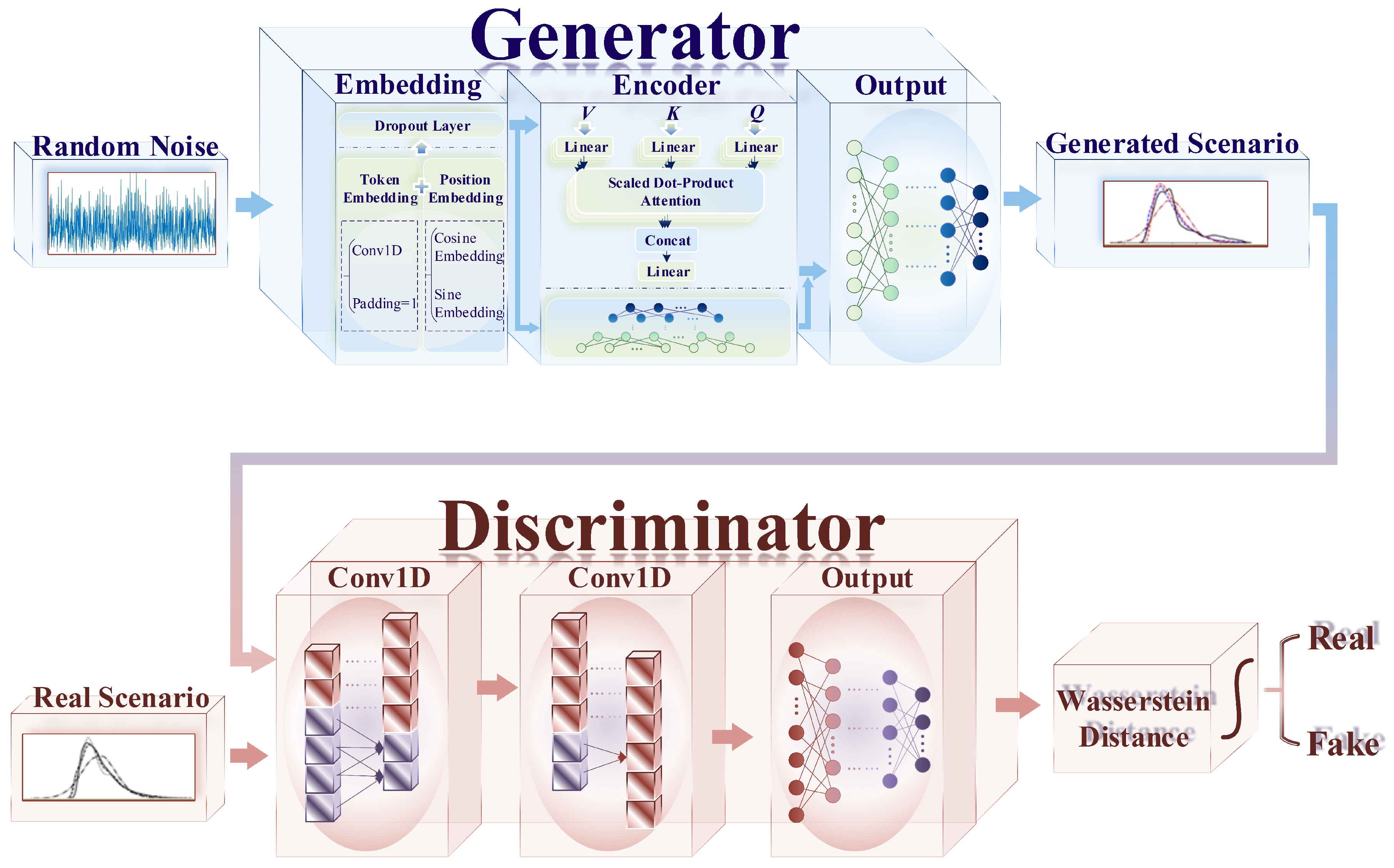Based on the WGAN-GP framework [33], the model is designed to incorporate a Transformer algorithm within the generator’s neural network architecture, which is illustrated in Figure 1.

The specific steps for generating renewable energy output scenarios based on the TWGAN-GP model are as follows:

• Collect and preprocess a substantial history dataset of renewable energy output;
• Input noise sampling from a Gaussian distribution into the generator to generate renewable energy output scenarios;
• Input both the model-generated and real output scenarios into the discriminator and then assess their resemblance based on the Wasserstein distance metric;
• Continuously optimize the generator and discriminator, ultimately achieving the effective generation of renewable energy output scenarios by the generator.

2.1. WGAN-GP: Integral Structure

The architecture of WGAN-GP primarily consists of the generative and discriminative units, which correspond to the model’s generator and discriminator, respectively.

• Generator: This generates samples based on noise data. It randomly samples noise data as its input from a Gaussian distribution, aiming to generate an output that closely mimics the distribution of real samples in the training set.
• Discriminator: This determines whether the received data are created by the generator. It is designed to differentiate between the real and the generated samples from the generator, with the goal of identifying the false data as accurately as possible.

Specifically, the generator takes a noise vector z as input, which is sampled from a recognized Gaussian distribution $P_{\mathrm{Noise}}$. Noise z is transformed by the generator into a set of random variables y, representing generated renewable energy output scenarios and belonging to a distribution denoted as $P_{\mathrm{Generate}}$, i.e., $y\sim P_{\mathrm{Generate}}$. The closer $P_{\mathrm{Generate}}$ is to $P_{\mathrm{Data}}$, the better the generated scenarios are at simulating the real scenarios.

$P_{\mathrm{Generate}}$ and $P_{\mathrm{Data}}$ are input into the discriminator concurrently and output a loss function value $W(P_{\mathrm{Data}},P_{\mathrm{Generate}})$ to measure the extent to which the generated samples $P_{\mathrm{Generate}}$ belong to the real samples $P_{\mathrm{Data}}$. Optimizing the model involves improving both the generator’s capacity to generate outputs that closely resemble real scenarios and the discriminator’s ability to determine the authenticity of the generated data. Throughout the training process, the discriminator continuously enhances its ability to maximize the differentiation between the generated and real data. The outcomes from the discriminator guide the generator in producing renewable energy output scenarios that more closely resemble real data. In the original GAN model, the procedure represented as a two-player game is characterized by a minimax strategy [34] as follows:

$$\underset{G}{\min }\underset{D}{\max }{V}_{\mathrm{ob}}(G,D)={\mathrm{E}}_{x\sim P_{\mathrm{Data}}}\left[\log D\left(x\right)\right]+{\mathrm{E}}_{y\sim P_{\mathrm{Generate}}}\left[\log (1-D\left(y\right))\right]$$

(1)

where the objective function of the discriminator is denoted as $V_{\mathrm{ob}}(G,D)$. It is worth noting that within Expression (1), the optimization problem for the discriminator is identical to the calculation of the Jensen–Shannon (JS) divergence between $P_{\mathrm{Generate}}$ and $P_{\mathrm{Data}}$. In most cases, where the distributions of generated and real samples do not overlap, the JS divergence may not effectively distinguish the distance between them but result in a consistent value-$\log 2$. This means that the JS divergence can only measure whether two distributions are similar, yet it falls short of quantifying the extent of their variance. In the context of renewable energy output scenario generation, it is essential for the generator to learn the real scenario distributions. If JS divergence is to be employed in the discriminator’s loss function, the model will exhibit a pronounced risk of gradient vanishing during the back-propagation process, generating a singular power distribution mode with the highest probability by the generator, thus leading to a decrease in the variety of generated samples. In order to address the challenges in training and mode-collapse issues caused by the application of JS divergence, WGAN-GP adopts the Wasserstein distance [35,36] as the discriminator’s loss function, which is defined as

$$\mathrm{W}(P_{\mathrm{Data}},P_{\mathrm{Generate}})=\underset{\gamma \in \Gamma (P_{\mathrm{Data}},P_{\mathrm{Generate}})}{\inf }{E}_{(x,y)\sim \gamma }\left[\right||x-y\left|\right|]$$

(2)

where the set $\Gamma (P_{\mathrm{Data}},P_{\mathrm{Generate}})$ consists of the joint distribution $\gamma (x,y)$ with marginal distributions of $P_{\mathrm{Generate}}$ and $P_{\mathrm{Data}}$. Sampling $(x,y)\sim \gamma$ is carried out from every potential joint distribution $\gamma (x,y)$ to acquire a real sample x and generated sample y before computing their distance $\left|\right|x-y\left|\right|$. Then, the Wasserstein distance is gained by taking the lower bound of the expectation of distances among samples across all potential joint distributions. The application of the Wasserstein distance is equal to resolving an optimal transport problem [27], namely, discovering the minimal distance required for the transportation of converting the distribution of generated scenarios $P_{\mathrm{Generate}}$ into the distribution of $P_{\mathrm{Data}}$. It computes the distance between $P_{\mathrm{Generate}}$ and $P_{\mathrm{Data}}$ directly even when they do not overlap, accurately delineating the discrepancy between their distributions and providing a precise training direction for the generator to fit a real distribution.

Additionally, the model proposed in this paper applies a gradient penalty factor as a substitute for enforcing Lipschitz constraints by directly constraining the gradient norm of the discriminator’s output relative to its input. In comparison with the weight-clipping method initially proposed by the WGAN, the approach of the gradient penalty factor for Lipschitz constraints can mitigate the difficulty of optimization and prevents the discriminator from exhibiting a pathological value surface [36]. The objective function of the discriminator is

$${WG}_{\mathrm{ob}}(G,D)=\underset{D}{\max }\{{\mathrm{E}}_{x\sim P_{\mathrm{Data}}}\left[D\left(x\right)\right]-{\mathrm{E}}_{y\sim P_{\mathrm{Generate}}}\left[D\left(y\right)\right]-\lambda {\mathrm{E}}_{x^{\prime }\sim P_{\mathrm{Penalty}}}\left[{({\left|\right|{\nabla }_{x^{\prime }}D\left(x^{\prime }\right)\left|\right|}_2-1)}^2\right]\}$$

(3)

where the gradient penalty term is calculated as $\lambda {\mathrm{E}}_{x^{\prime }\sim P_{\mathrm{Penalty}}}\left[{({\left|\right|{\nabla }_{x^{\prime }}D\left(x^{\prime }\right)\left|\right|}_2-1)}^2\right]$ and $\lambda$ represents the penalty coefficient. $P_{\mathrm{Penalty}}$ is defined as uniform sampling along the line connecting pairs of points from $P_{\mathrm{Data}}$ to $P_{\mathrm{Generate}}$. Sampling $x^{\prime }$ from the probability distribution $P_{\mathrm{Penalty}}$ is expressed as $x^{\prime }\sim P_{\mathrm{Penalty}}$. Additionally, ${\nabla }_{x^{\prime }}D\left(x^{\prime }\right)$ is the derivative (gradient) of the discriminator’s output $D\left(x^{\prime }\right)$ with respect to its input $x^{\prime }$.

2.2. Transformer: Temporal Characterization

At present, the generators and discriminators in most GAN-based models aim to utilize the CNN architecture. The CNN excels in the domain of image processing due to its ability to extract data features through the convolutional kernels. However, it falls slightly short in its ability to capture the timing characteristics, considering that the scenario data in this study are time series, which exhibit strong temporal correlations and long-distance dependencies. Meanwhile, the self-attention mechanism within Transformer [37] is capable of calculating feature correlations between any two positions, proving more effective in processing long sequential time-series data compared to models like the CNN and LSTM. Consequently, this study enhances the structure of the generator’s internal network based on the Transformer algorithm, enabling it to better capture the long-distance dependencies between renewable energy output scenarios.

The specific structure of Transformer is depicted in the generator section of Figure 1. Combined with the specific characteristics of the actual demand, which need to generate scenarios from noise data without the demand for a full encoding–decoding process, only the encoding component of Transformer is utilized. As the core modules, Embedding and Encoder, respectively, implement a representation of the input data and the Multi-Head Self-Attention (MHSA) mechanism. The output of MHSA is connected to a Multi-Layer Fully Connected Neural Network (MLFCNN). The residual network between Embedding and the Feedforward network is employed to effectively extract and utilize data feature information. The extracted results are ultimately combined with the output of MHSA and fed into the Output module, where the data dimensions are adjusted via an MLFCNN and accomplish the generation of renewable energy output scenarios.

2.2.1. Input Data Representation—Embedding Module

In order to enhance the ability of Transformer to precisely capture the temporal correlations among wind power and PV scenarios, positional encoding to the renewable energy output data is performed as follows:

$$X_{\mathrm{Embedding}}^{\mathrm{T}}=X+PE\left(X\right)$$

(4)

where X represents the original time series, $X_{\mathrm{Embedding}}^{\mathrm{T}}$ is the renewable energy data after time embedding, and $PE\left(X\right)$ signifies position embedding, which is expressed by the following equation:

$$\left\{\begin{array}{c}P{E}_{(\mathrm{position},2j)}\left(X\right)=\sin \left({\displaystyle \frac{\mathrm{position}}{{\mathrm{10,000}}^{2j/d_{\mathrm{model}}}}}\right)\hfill \\ P{E}_{(\mathrm{position},2j+1)}\left(X\right)=\cos \left({\displaystyle \frac{\mathrm{position}}{{\mathrm{10,000}}^{2j/d_{\mathrm{model}}}}}\right)\hfill \end{array}\right.$$

(5)

where position denotes the absolute position of this element within the time series, $d_{\mathrm{model}}$ represents the dimension of $PE\left(X\right)$, $2j$ stands for the dimensional size of the feature vector associated with even numbers, and $2j+1$ corresponds to the size of the feature vector related to odd numbers (i.e., $2j\le d_{\mathrm{model}}$, $2j+1\le d_{\mathrm{model}}$).

2.2.2. MHSA—Encoder Module

The $X_{\mathrm{Embedding}}^{\mathrm{T}}$ obtained by the Embedding module is multiplied by the weight matrices $W_{\mathrm{Q}}$, $W_{\mathrm{K}}$, and $W_{\mathrm{V}}$ to yield the corresponding vectors Q, K, and V. MHSA is realized by dot product mapping between Q, K, and V. The computation process is as follows:

$$\mathrm{Attention}(Q,K,V)=\mathrm{softmax}\left({\displaystyle \frac{Q{K}^{\mathrm{T}}}{\sqrt{d_{Key}}}}\right)V$$

(6)

First, a dot product is calculated between Q and K for the weight of similarity, which is then divided by $\sqrt{d_{\mathrm{Key}}}$, where $d_{\mathrm{Key}}$ represents the dimension of vector Key, to prevent excessively large outcomes. Then, a softmax function normalizes these results to a probability distribution. After that, the normalized weight is multiplied by the value corresponding to the key to obtain the weight sum representation. Within the MHSA framework, the process above is replicated for each attention head. Mapping Q, K, and V through n distinct linear transformations before concatenating various attentions, a linear transformation is performed in the end. The formula is presented below:

$$\mathrm{MultiHead}(Q,K,V)=\mathrm{Concat}({\mathrm{head}}_1,{\mathrm{head}}_2,\dots ,{\mathrm{head}}_n)W_{\mathrm{O}}$$

(7)

$${\mathrm{head}}_j=\mathrm{Attention}(Q{W}_{\mathrm{Q},j},K{W}_{\mathrm{K},j},V{W}_{\mathrm{V},j})$$

(8)

where $W_{\mathrm{Q},j}\in R^{d_{\mathrm{model}}\times d_{\mathrm{Key}}}$, $W_{\mathrm{K},j}\in R^{d_{\mathrm{model}}\times d_{\mathrm{Key}}}$, $W_{\mathrm{V},j}\in R^{d_{\mathrm{model}}\times d_{\mathrm{Value}}}$, $W_O\in R^{n{d}_{\mathrm{Value}}\times d_{\mathrm{model}}}$, $d_{\mathrm{Value}}$ denotes the dimension of vector V, and n is the number of attention heads, while $\mathrm{Concat}(·)$ stands for the operation of concatenating output vectors from these heads into a long vector in sequence.

Noting that the generator of TWGAN-GP employs a Transformer architecture for its internal algorithm, the network of the discriminator integrates two CNNs with an MLFCNN. The input of the generator is Gaussian noise. When the data enter the generator, the generator first embeds feature and positional information through the Embedding module before they are concatenated and input into the Encoder module for MHSA calculation. In the meantime, the splicing result from the Embedding module goes through an MLFCNN as well. The operations are performed multiple times before two results from the Encoder module are input into the Output module together to adjust the dimension of data through an MLFCNN and to map the data to the generated renewable energy output scenario distribution. The discriminator receives both real and generated output scenarios, with the data processing through two sequential CNNs and entering into the Output module where the MLFCNN adjusts the dimension of the data to produce the Wasserstein distance, reflecting the authenticity of renewable energy scenarios.

3. Case Study

For the case study, 44,895 samples are derived from the California 2006 Photovoltaic Output Dataset [38] and the Wind Integration National Dataset (WIND) [39], both of which are accessible to the public from the National Renewable Energy Laboratory (NREL). The collected samples are preprocessed with a random division process that splits them into training and test sets in a ratio of 8:2. The experimental platform is developed on a Linux server, equipped with an RTX 3090 GPU (24 GB) and CUDA version 11.3. The programming is conducted in Python version 3.9, with PyTorch 1.11.0 serving as the deep learning platform.

Table 2. Hyper-parameters of TWGAN-GP model.

Hyper-Parameters	Wind Power	PV
Dimension of Transformer Embedding Layer	128	128
Dimension of Transformer Feedforward Layer	256	1024
Number of Attention Heads	8	4
Sequence Length	24	24
Gradient Penalty Weight	10	10
Learning Rate	0.0001	0.0001
Batch Size	256	256
Noise Dimension	100	100

gives the hyper-parameters for TWGAN-GP. To analyze the efficacy of the proposed model, WGAN-GP and VAE are selected for comparison. In addition, considering that TWGAN-GP, like WGAN-GP and VAE, belongs to the data-driven model mentioned in the introduction, the Copula function and LHS, two classic model-driven methods, are introduced for comparative experiments to ensure the analysis is more convincing and comprehensive. The chosen dataset, on the one hand, is used to train and optimize TWGAN-GP, WGAN-GP, and VAE and, on the other hand, is employed to fit the distribution parameters of the prior distributions selected by the Copula function and LHS, respectively. Then, each model produces 10,000 samples of renewable energy output scenarios for the effectiveness assessment.

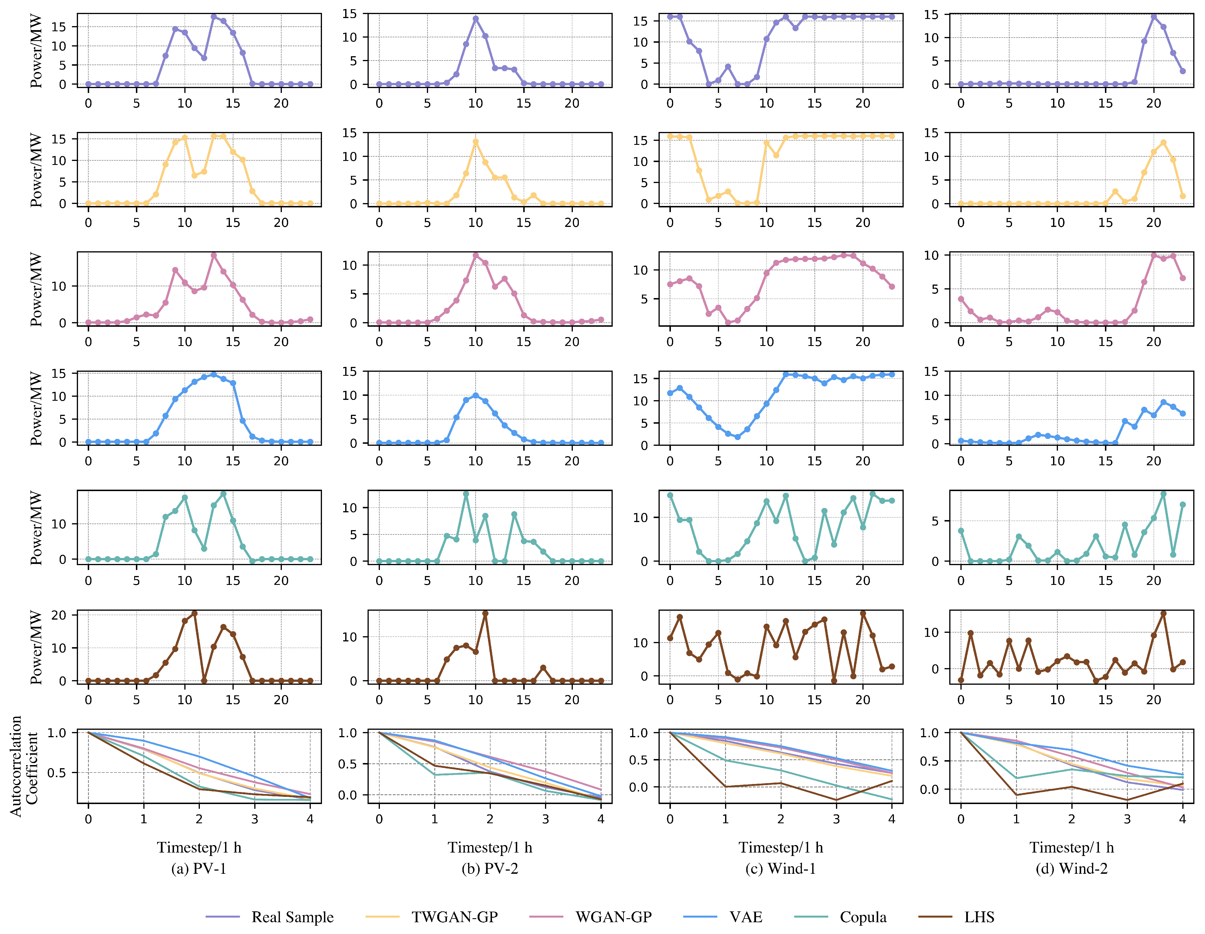
First, a qualitative comparison focusing on the perspective of individual samples of model-generated scenarios is conducted in Figure 2. Two output curves are extracted from the real wind power and PV output scenarios. Then, the output samples with the shortest Euclidean distance to the real samples are selected from the scenario sets generated by TWGAN-GP, WGAN-GP, VAE, the Copula function, and LHS before calculating their temporal correlations correspondingly. Figure 2a,b compare the curves of real PV output samples with the selected scenarios generated by each model according to the closest Euclidean distance, as well as their respective temporal correlations. Similarly, Figure 2c,d show the same comparison for wind power output scenarios. It is evident that, in comparison to WGAN-GP, VAE, the Copula function, and LHS, TWGAN-GP, whose generated output curves more closely resemble those of the real scenarios, outperforms in capturing the fluctuation and uncertainty characteristics of wind power and PV outputs. Additionally, TWGAN-GP presents a much closer alignment with real samples in terms of temporal correlation.

The following content describes a comprehensive comparison of model performance based on various evaluation indexes: expectation and variance, the probability density function (PDF), the cumulative distribution function (CDF), power spectral density (PSD), temporal correlation, and pinball loss. It is worth mentioning that, unlike the general supervised learning models whose calculation of indicators for evaluating their performance involves a comparison of the difference between the model output and the label of the corresponding single real sample one by one, the main task of our scenario generation model is to fit the probability distribution of the real dataset. Since the training and test sets are sampled from the same data source, they conform to the same distribution so that their various statistical indexes are consistent as well. Therefore, the following analyses basically focus on contrasting the ability of renewable energy scenarios generated by each model to fit the statistical characteristics and distributional properties of real samples from the perspective of curve and quantitative data analyses.

3.1. Expectation and Variance

In statistics, the dissimilarity of the moment can measure the similarity of two probability distributions. This study uses expectation to reflect the average output level of the scenario set and variance to assess the variety within samples. By comparing these metrics of each scenario set, the adaptability of each scenario generation model to describe the average statistical characteristics and output fluctuation characteristics of the real renewable energy output can be measured, respectively. Assume that the scenario set $\mathbf{Y}=\left\{{\mathit{y}}_i\right\},i=1,2,3,\dots ,N$ contains N scenarios, denoted as ${\mathit{y}}_i=\left\{y_t\right\},t=1,2,3,\dots ,T$. $y_t$ is the feature value of scenario ${\mathit{y}}_i$ at a given time t. The time dimension of each scenario is symbolized as T. The formulas of expectation and variance are as follows:

$$\mathit{\mu }={\displaystyle \frac{{\sum }_{i=1}^N{\mathit{y}}_i}{N}}$$

(9)

$${\mathit{\sigma }}^2={\displaystyle \frac{{\sum }_{i=1}^N{({\mathit{y}}_i-\mathit{\mu })}^2}{N}}$$

(10)

where $\mathit{\mu }$ represents the expectation, while $\mathit{\sigma }$ denotes the standard deviation of the scenario set.

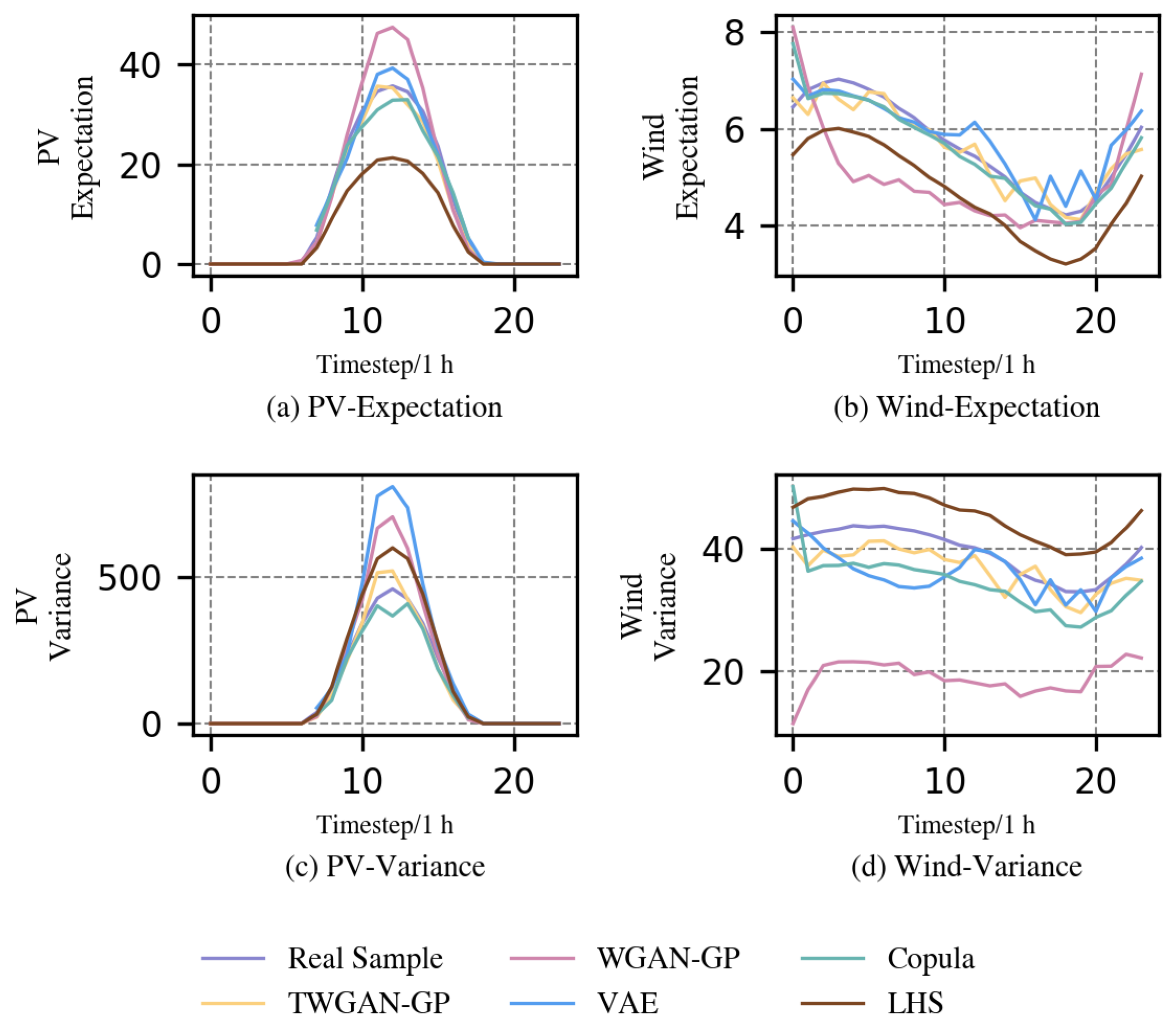
Figure 3 depicts the expectations and variances of the real scenarios and the generated scenarios of each model. First, it is evident that LHS and WGAN-GP generally do not perform well in every chart of Figure 3 in comparison with other models, which means both of them lack the ability to follow the statistical properties of expectation and variance of renewable energy output scenarios. In terms of expectation, the curve of the Copula function in the wind power scenarios basically coincides with the expectation of the real sample, while TWGAN-GP shows the best fitting ability for the real wind power samples in the PV scenarios. TWGAN-GP and the Copula function follow the variance–characteristic curve of the real PV scenarios in a similar way, and both show the best fitting ability among all models. Under the variance indicator of the wind power scenarios, the Copula function performs relatively poorly, especially during the starting time step, where there is a large numerical gap with the real samples. VAE demonstrates the lowest performance in terms of PV variance. Moreover, it is noticed that for wind power scenarios, compared to the poorer fitting ability of VAE to real samples at certain time points (e.g., the significant fluctuation in the expectation curve of VAE after 10 h; completely opposite trends in the variance curve of VAE to that of the real sample during the period of 1–12 h), the curve of TWGAN-GP, despite some minor fluctuations, still aligns more closely overall with the trend of real scenarios. In general, although VAE and the Copula function also have excellent performance in some cases, they show poor effects in some special results. By contrast, the scenario data generated by TWGAN-GP show a very appropriate description of the real samples in terms of both expectation and variance, whether in the situation of wind power or PV. Hence, Figure 3 demonstrates the capability of TWGAN-GP to create more authentic scenarios for renewable energy output.

3.2. PDF

The PDF quantifies the consistency and accuracy between the generated and real scenarios by outlining the probability of the output of renewable energy near a specific power point. The PDF curves can directly display the distribution differences among different scenario sets at each output point [21]. The calculation process of the PDF is as follows:

• Divide the power range covered by the scenario set into M equal-width intervals, with each interval width denoted as $\Delta m$ and the center point of the interval denoted as $\Delta m_i$;
• Calculate the number of times the data in the scenario set appear in the interval $\Delta m$, denoted as $f_i,i=1,2,3,\dots ,M$;
• Calculate the PDF as

  $$\mathrm{PDF}(\Delta m_i)={\displaystyle \frac{f_i}{S·\Delta m}}$$

  (11)

  where S is the total number of samples in the scenario set, while $\mathrm{PDF}(\Delta m_i)$ signifies the probability density of the scenario set at $\Delta m_i$.

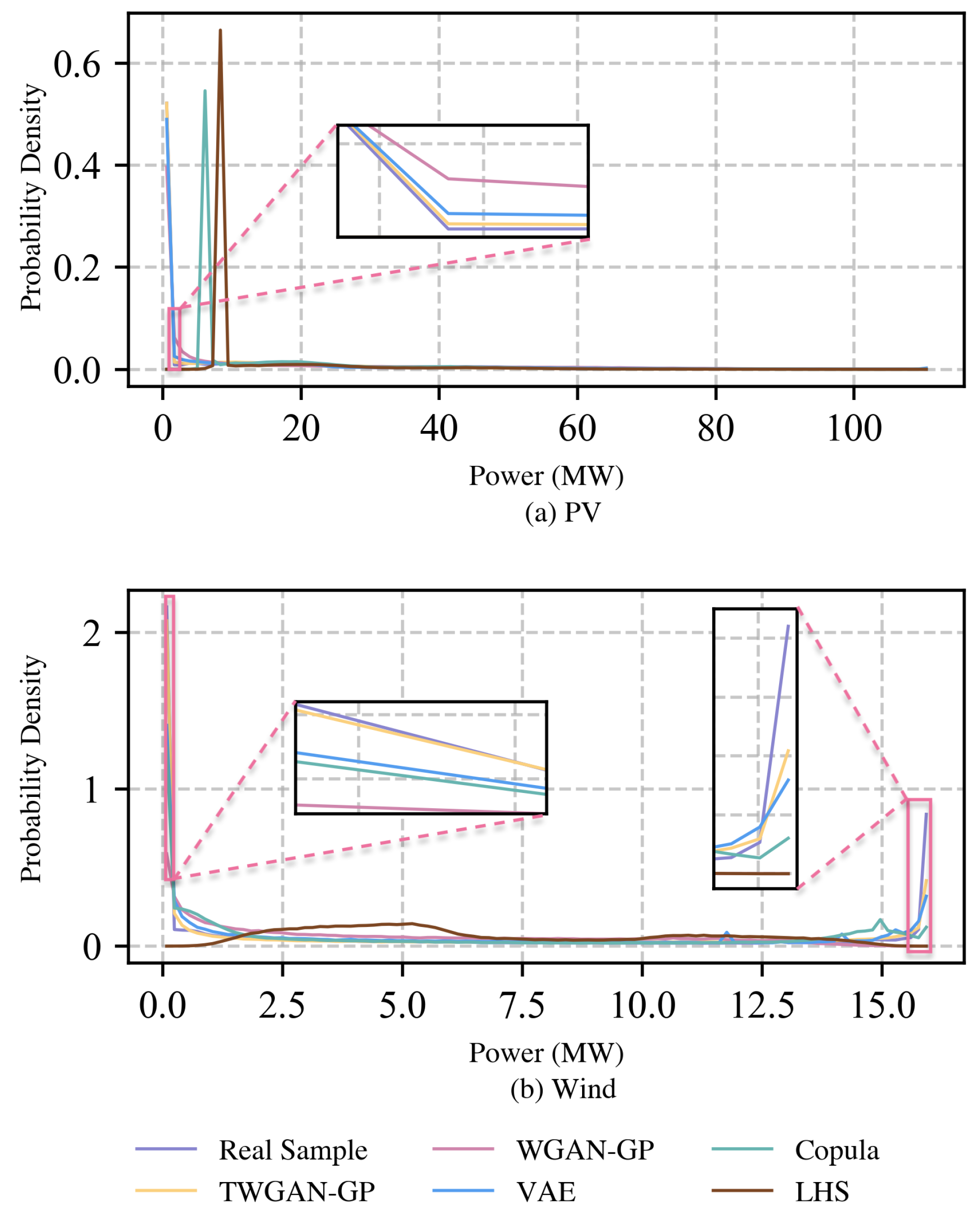
Figure 4 illustrates the PDF curves of real renewable energy output scenarios and those generated by different models, with (a) pertaining to PV and (b) to wind power. To facilitate a comparative observation of the efficacy of model-generated scenario sets from the perspective of probability density, Figure 4 presents detailed examinations of the PDF curves for PV output within the power range of 1.4∼2.0 MW and the probability density interval of 0∼0.12, as well as wind power output within the power ranges of 0.08∼0.16 and 15.5∼15.97 MW and the probability density intervals of 0.45∼2.2 and −0.05∼0.9. It is worth mentioning that the choice of −0.05 is made for the convenient observation of WGAN-GP and LHS, whose PDF curves corresponding to the wind power scenarios are infinitely close to zero within the power range of 15.5∼15.97 MW. First, a very clear phenomenon that can be easily observed from the big-view diagram is that the PDFs of two model-driven probability models, the Copula function and LHS, in the PV scenario are quite poor, with their probability density peaks at 6 and 8 MW, respectively, which are absent in the probability density distribution curve of the real samples. In the case of wind power, the fitting capacity of the scenarios generated by LHS is still significantly inferior to that of other models. In comparison, the PDF curve of the Copula function, except for the small bump near 15 MW, has better overall performance, but it is still not as good as the dataset generated by the data-driven model in following the real scenarios in terms of the PDF indicator. Then, from the magnified views of the PDF curves within the power interval of 1.4∼2.0 MW and probability density interval of 0∼0.12 for PV scenarios, and that within the power interval of 0.08∼0.16 MW and probability density interval of 0.45∼2.2 for wind power scenarios, it is evident that the PDF curve of the generation scenarios of the proposed TWGAN-GP model is infinitely close to that of real scenarios in both intervals. By contrast, the WGAN-GP and VAE exhibit slight deficiencies. Although the performance of TWGAN-GP in wind power scenarios within the power range of 15.5∼15.97 MW and the probability density interval of −0.05∼0.9 is slightly inferior to the presentation in the two aforementioned intervals, it still outperforms other comparative models. From the perspective of the PDF, the model proposed in this paper can generate scenarios that better match the authentic probability distributions of PV and wind power outputs compared to the comparison models, representing the benefits brought by Transformer in capturing the temporal features of renewable energy output scenarios. Notably, in three principal intervals, the traditional WGAN-GP exhibits the poorest PDF performance among three data-driven probability models presented here, which also shows that the advancement of WGAN-GP has a significant positive effect on improving its performance.

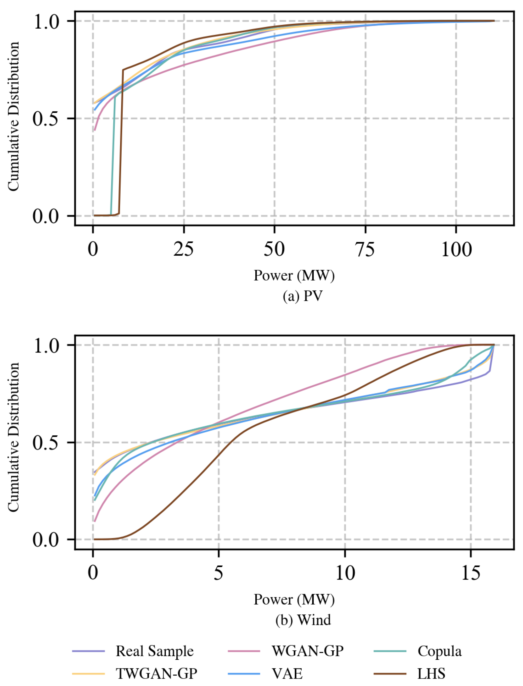
3.3. CDF

The CDF is the integral of the PDF. It can fully describe the probability distribution of a scenario dataset, thereby evaluating the model’s capacity to simulate the real renewable energy output by comparing the distribution differences between the scenarios they generated and the real output samples. The calculation formula of the CDF is as follows:

$${\displaystyle \mathrm{CDF}(\Delta m_i)=\sum _{j=1}^i\mathrm{PDF}(\Delta m_j)·\Delta m}$$

(12)

where $\mathrm{CDF}(\Delta m_i)$ represents the cumulative distribution value of the scenario set at $\Delta m_i$.

The CDF curve of all scenario datasets under the PV scene is given in Figure 5a, while Figure 5b presents the results in the wind power scene. It is seen that, in PV scenario generation, the two model-based methods perform clearly more poorly than the data-driven models, as, in the starting power range of 0∼20 MW, the CDF curves of the Copula function and LHS show a clear inconsistency compared to the others and even exhibit a CDF result of 0 in the range of 0∼10 MW. As for the data-driven models, in the 0∼50 MW power range, compared with WGAN-GP, TWGAN-GP and VAE both almost show a great ability to follow the general shape of real samples. However, when the power increases to 50 MW, the advantage of TWGAN-GP is clearer. Excluding the range after about 90 MW where all CDFs reach 1.0, it can be seen that the fitting effect of TWGAN-GP on the real PV output is relatively excellent when generating PV scenarios. It cannot be ignored that in the wind power scene, the Copula function shows an excellent ability to fit the probability distribution of the real scenario output, although the performance of LHS is still poor, with the 0 probability value occurring in the range of 0∼1.5 MW. Within 0∼10 MW, the CDF curves of the TWGAN-GP-generation and real wind power datasets are basically completely overlapped. After that, as the power increases, the curves of TWGAN-GP and VAE are consistent, where there are slight deviations from the real samples. It is worth noting that in the three data-driven models, whether in the wind power or PV scenarios, the ability of WGAN-GP to describe the probability distribution of real samples is overall inferior. Based on the analysis above, in terms of the CDF index, the performance of TWGAN-GP indicates a positive effect of improving its simulation ability for the marginal distributions of real renewable energy output with the help of Transformer.

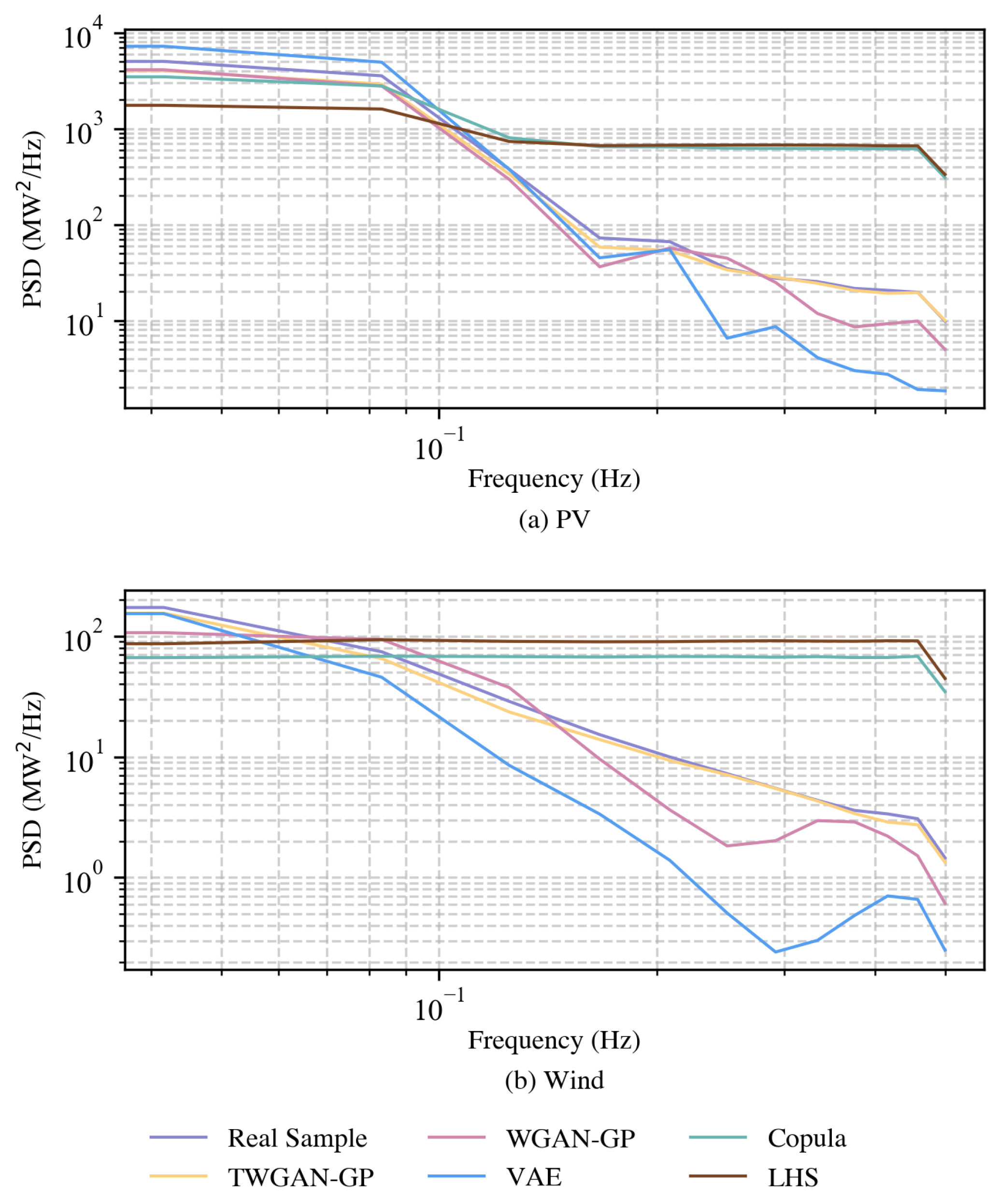
3.4. PSD

To more comprehensively verify the effectiveness and accuracy of the TWGAN-GP model in generating renewable energy output scenarios, in addition to the time-domain analysis for datasets, this study also considers applying the PSD indicator to measure the similarity of frequency-domain characteristics between the generated scenarios and the real samples. PSD is a measure of the mean square value of power within a unit frequency band, reflecting the power distribution characteristics of the time series, the renewable energy output in this study, in the frequency aspect. Its calculation process involves, first, calculating PSD for each time-series dataset with the Welch method:

$$\mathrm{PSD}\left(f\right)={\displaystyle \frac{1}{N}}{\left|\mathcal{F}\left(x\left(t\right)\right)\right|}^2$$

(13)

where $\mathcal{F}\left(x\right(t\left)\right)$ is the Fourier transform of the time series $x\left(t\right)$, and N is the number of time steps. Then, the PSD of all samples is averaged as

$${\displaystyle \overline{{\mathrm{PSD}}_{\mathrm{Real}}}\left(f\right)=\frac{1}{n}\sum _{i=1}^n{\mathrm{PSD}}_{\mathrm{Real},i}\left(f\right)}$$

(14)

$${\displaystyle \overline{{\mathrm{PSD}}_{\mathrm{Generate}}}\left(f\right)=\frac{1}{m}\sum _{j=1}^m{\mathrm{PSD}}_{\mathrm{Generate},j}\left(f\right)}$$

(15)

where n and m are the number of samples of real and generated data, respectively.

The corresponding results of the PSD calculation are plotted in Figure 6. From the frequency-domain perspective, the Copula function and LHS hardly follow the power distribution features of real scenarios. Although the trends of three data-driven models are basically consistent with the real samples, the ability of TWGAN-GP to capture the power distribution characteristics of the real samples in the frequency domain is still evident since its PSD curve is nearly coincident with that of the real one. Compared to the comparison models, TWGAN-GP shows a better ability to fit real samples in terms of the PSD index.

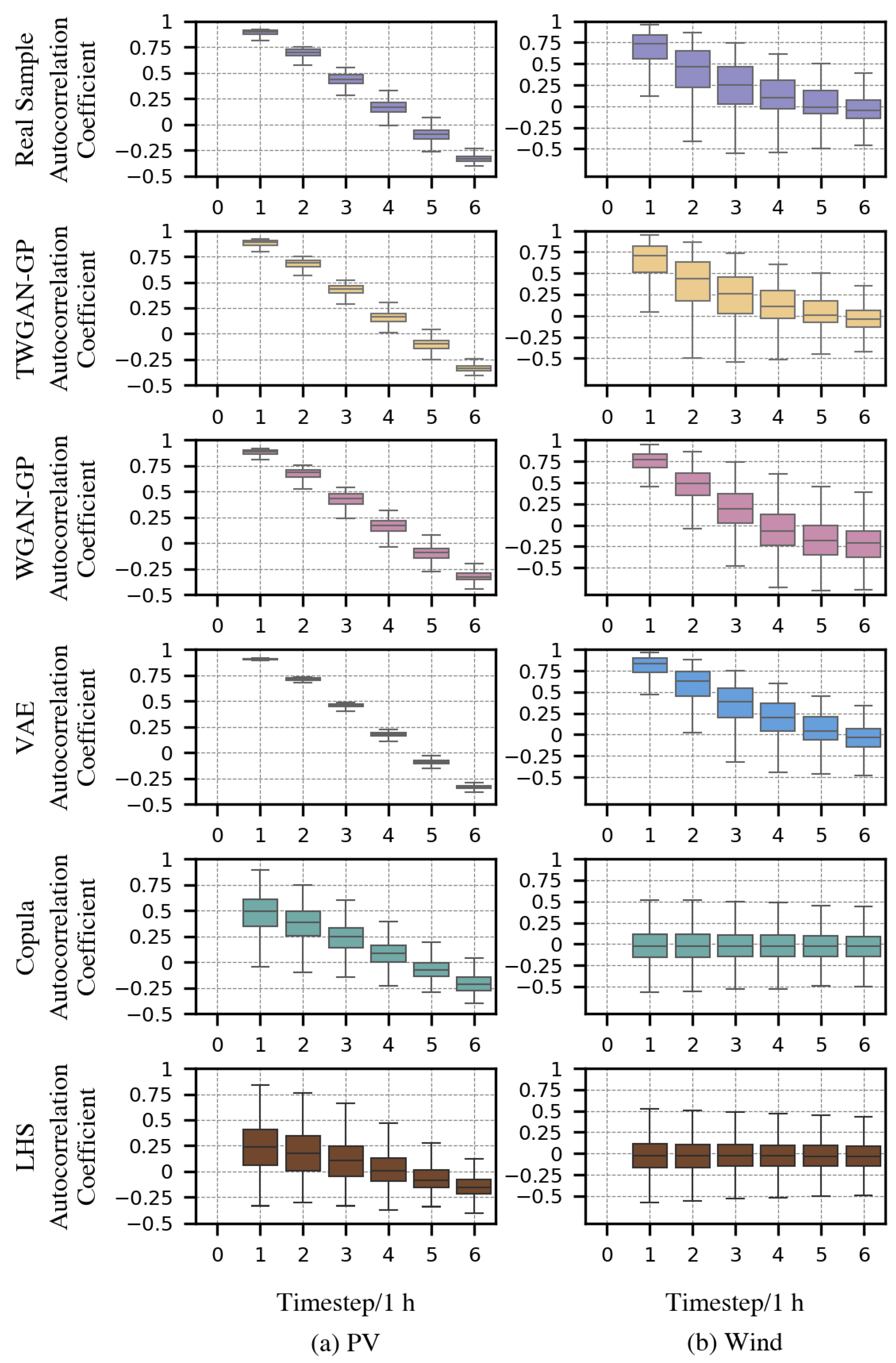
3.5. Temporal Correlation

Renewable energy displays a certain level of temporal correlation at various moments. To gauge the modeling effect of different models on the temporal correlation of renewable energy output, the autocorrelation coefficient $\mathrm{Y}\left(\xi \right)$ is employed in this study. This coefficient reflects the internal time-series characteristics of the dataset by calculating the correlation between two renewable energy outputs at different lag time points. Therefore, by analyzing the size and changing features of the autocorrelation coefficients, and assessing the alignment between generated and real scenarios in terms of temporal correlation, the quality of the generated scenarios can be evaluated. The formula is as follows:

$$\mathrm{Y}\left(\xi \right)={\displaystyle \frac{\mathrm{E}\left[(y_t-\mu )(y_{t+\xi }-\mu )\right]}{{\sigma }^2}}$$

(16)

where $y_t$ is the value of renewable energy output at time t, $\xi$ represents the lag time of the output scenario, $\mu$ signifies the expectation of renewable energy outputs, and their standard deviation is represented as $\sigma$.

Figure 7a,b depict boxplots of the autocorrelation coefficients relating to real and model-generation scenarios of PV and wind power at various lag times, respectively. It is observed that the Copula function and LHS are worst in describing the autocorrelation coefficient of real scenarios, which signifies that they can hardly capture any time correlation features of real samples. Especially in the wind power situation, their boxplots barely change with the variance in the lag time. This almost indicates that the scenarios they generated completely ignore the simulation of internal time correlation properties of renewable energy output. For data-driven models, it is apparent that the performance of PV scenarios generated by VAE in terms of temporal correlation is suboptimal, evidenced by a noticeable discrepancy in its boxplot in comparison with the temporal correlation pattern of real data. Meanwhile, in the case of wind power scenarios at lag times 1∼4, the autocorrelation coefficient distributions of VAE present clear differences at the upper/lower margins, upper/lower quartiles, and median part against the boxplots of real scenarios. As for WGAN-GP, in PV scenarios, the distribution of the autocorrelation coefficient significantly differs from the real scenarios at the sixth lag, where its upper and lower edge ranges are substantially larger than those of the real one. For wind power scenarios, its corresponding autocorrelation coefficients at lag times 1, 2, 4, 5, and 6 are clearly distinct from real scenarios as well. Conversely, TWGAN-GP possesses a higher capability in mirroring the temporal correlations of both the wind power and PV output observed in the real scenario set. Compared with WAGN-GP, it is reasonable to believe that the reason TWGAN-GP outperforms in fitting the temporal correlation of real scenarios is because of the support of the Transformer algorithm.

In addition to visually observing the temporal correlation between various datasets in boxplots, the Kolmogorov–Smirnov (K-S) statistical test is conducted to quantify the significance of the disparities between the autocorrelation coefficient distribution of the datasets from each generative model and the real samples. The results reveal that at the 5 and $10\%$ significance levels, TWGAN-GP, WGAN-GP, and VAE can pass the K-S test, while the Copula function and LHS cannot, which also demonstrates that, even in a statistical sense, there is no notable dissimilarity between the time-dependent feature distribution of data generated by TWGAN-GP and that of the real samples at the 5 and $10\%$ significance levels, indicating a strong correlation.

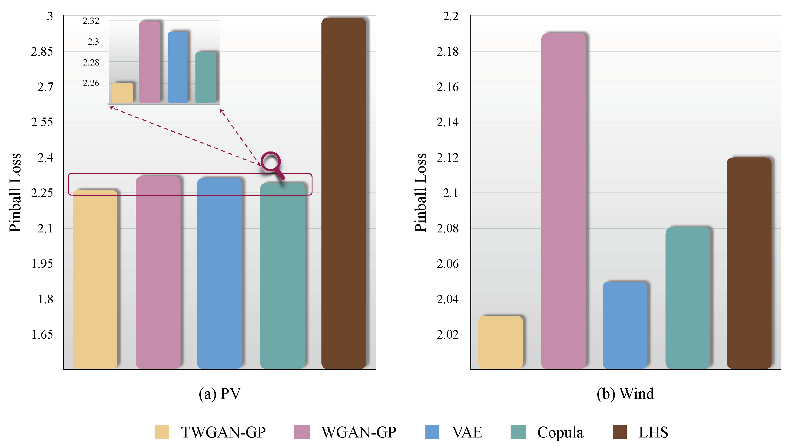
3.6. Pinball Loss

The pinball loss calculates the error between renewable energy generation scenarios and real scenarios based on quantiles. Unlike the expectation and variance, it can focus on any position in the distribution through different quantiles, providing a more comprehensive quantitative evaluation of the accuracy and effectiveness of the generated scenario distribution. A smaller pinball loss indicates a more accurate and effective generation. The computation process for the pinball loss is

$$P(M,N)=\left\{\begin{array}{c}{\displaystyle \frac{{\sum }_{i=1}^q({\beta }_i-1)(M_{\mathrm{Real}}-N_{{\beta }_i})}{q},M_{\mathrm{Real}}<N_{{\beta }_i}}\hfill \\ {\displaystyle \frac{{\sum }_{i=1}^q{\beta }_i(M_{\mathrm{Real}}-N_{{\beta }_i})}{q},M_{\mathrm{Real}}>N_{{\beta }_i}}\hfill \end{array}\right.$$

(17)

$$P={\displaystyle \frac{{\sum }_{t=1}^{T}P(M_t,N_t)}{T}}$$

(18)

where $P(M_t,N_t)$ signifies the value of pinball loss in the renewable energy scenario at a specific moment t, $M_{\mathrm{Real}}$ is the real output value of PV and wind power, and $N_{{\beta }_i}$ represents the value of the renewable energy output corresponding to the $i^{th}$ quantile. q indicates the number of quantiles, and ${\beta }_i$ represents the i-th quantile.

In this study, the pinball loss index is set to four quantiles, which are 20, 40, 60, and 80%. By calculating the pinball loss on each quantile and weighted summation, the comparison results of Figure 8 are obtained. Figure 8a shows the bar chart of pinball loss for TWGAN-GP, WGAN-GP, VAE, the Copula function, and LHS in PV scenarios, while Figure 8b shows the bar chart of pinball loss for various models in the wind power scenarios. It is clear that in the PV scenarios, LHS has a significantly larger pinball loss, which is $2.99$ compared with other models whose values of pinball loss are basically distributed around $2.3$. Furthermore, we locally amplify the pinball loss histograms of TWGAN-GP, WGAN-GP, VAE, and the Copula function to highlight their discrepancies. In the zoomed-in diagram, we can clearly see the superiority of TWGAN-GP, with the smallest pinball loss of $2.26$. Under the case of wind power, WGAN-GP reveals the highest pinball loss, which is $2.19$, while the scenario dataset generated by TWGAN-GP still outperforms among the five models as expected, with a value of $2.03$, the lowest pinball loss. This illustrates that the improvement in the algorithm in the WGAN-GP generator based on Transformer has enhanced the accuracy and effectiveness of WGAN-GP in generating renewable energy output scenarios.

The above results indicate that compared to the traditional models in all indicators, the proposed model generates more accurate short-term renewable energy output scenarios, demonstrating better performance.

4. Conclusions

In response to the challenging issue of modeling the uncertainty and randomness in renewable energy output, this paper proposes TWGAN-GP, which improves the performance of GANs in generating sequential data by integrating the Transformer architecture with the WGAN-GP framework. Through a detailed comparative analysis of the performance of generation models with two classic data-driven methods, WGAN-GP and VAE, and two traditional model-driven models, the Copula function and LHS, based on an open-source wind power and PV dataset, the effectiveness and precision of TWGAN-GP are confirmed according to several evaluation indicators. In contrast to the four comparison models mentioned above, TWGAN-GP has comparative advantages in single-sample feature comparison, expectation and variance, the PDF, the CDF, PSD, the autocorrelation coefficient, and pinball loss, and it is capable of generating scenarios that better match the real renewable energy output.

The renewable energy output scenarios generated by TWGAN-GP can effectively assist power operators in exhibiting more authentic output characteristics of renewable energy stations. For its possible practical applications in the real-world energy sector and modern power system, the following practical recommendations are given:

• On the one hand, the renewable energy output scenarios generated by TWGAN-GP can be used for a more precise analysis of the actual power balance situations in the power system across distinct time and space, providing more reliable support for power operators to make investment plans. For example, when making investment decisions for the location and capacity of transformers or energy storage equipment, the generated scenarios with more authentic properties can provide more precise information for decision makers, thereby improving the operational efficiency for operators.
• On the other hand, combined with the massive renewable energy output scenarios generated by TWGAN-GP, which can provide strong data support, the training of data-based optimization scheduling and planning models can be more effectively conducted. This helps the data-driven models learn and capture the uncertainty and randomness of renewable energy output more accurately, thereby enhancing the reliability and generalization ability of the decision-making solutions they provide and improving the intelligence level of system scheduling.

However, there are still limitations in TWGAN-GP:

• This study focuses on modeling the temporal characteristics of renewable energy output. However, in real situations, the outputs among multiple renewable plants in the power system are not only temporally correlated but also spatially correlated. Therefore, the model proposed in this paper is not suitable for collective scenario generation between various plants. The following research aims to integrate the Conditional GAN method into TWGAN-GP to improve its generation performance in the abovementioned case.
• It is worth noting that TWGAN-GP is a deep learning-based model. In the case of newly built renewable plants with insufficient historical data, it is not easy to train TWGAN-GP effectively. Therefore, the next step is to work on the scenario generation of renewable plants with insufficient data based on transfer learning and TWGAN-GP.