
Remote Sensing of Residential Landscape Irrigation in Weber County, Utah: Implications for Water Conservation, Image Analysis, and Drone Applications


Abstract
1. Introduction
2. Materials and Methods
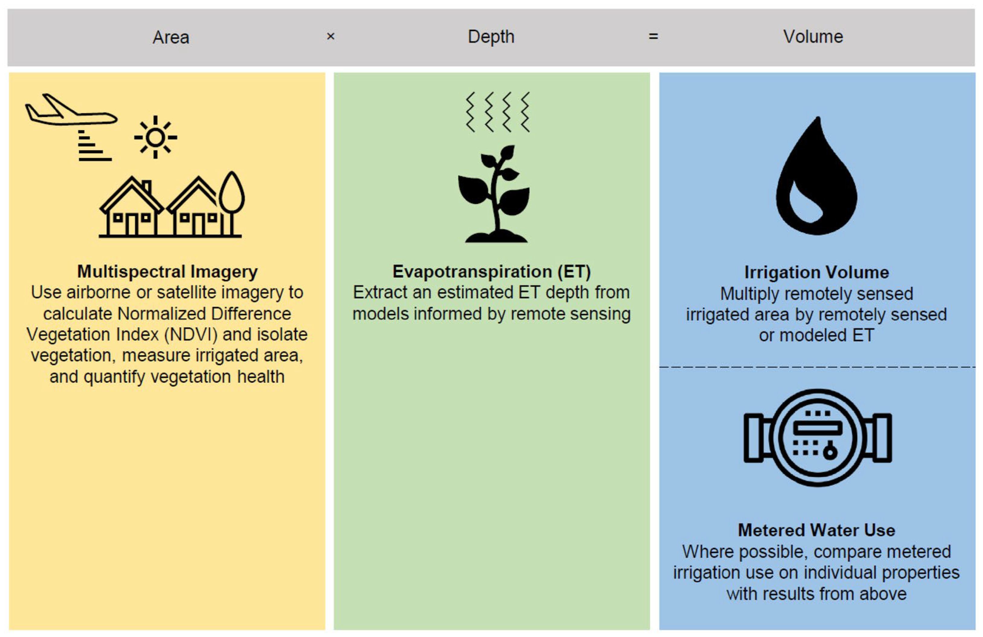
2.1. General Approach with AIRS
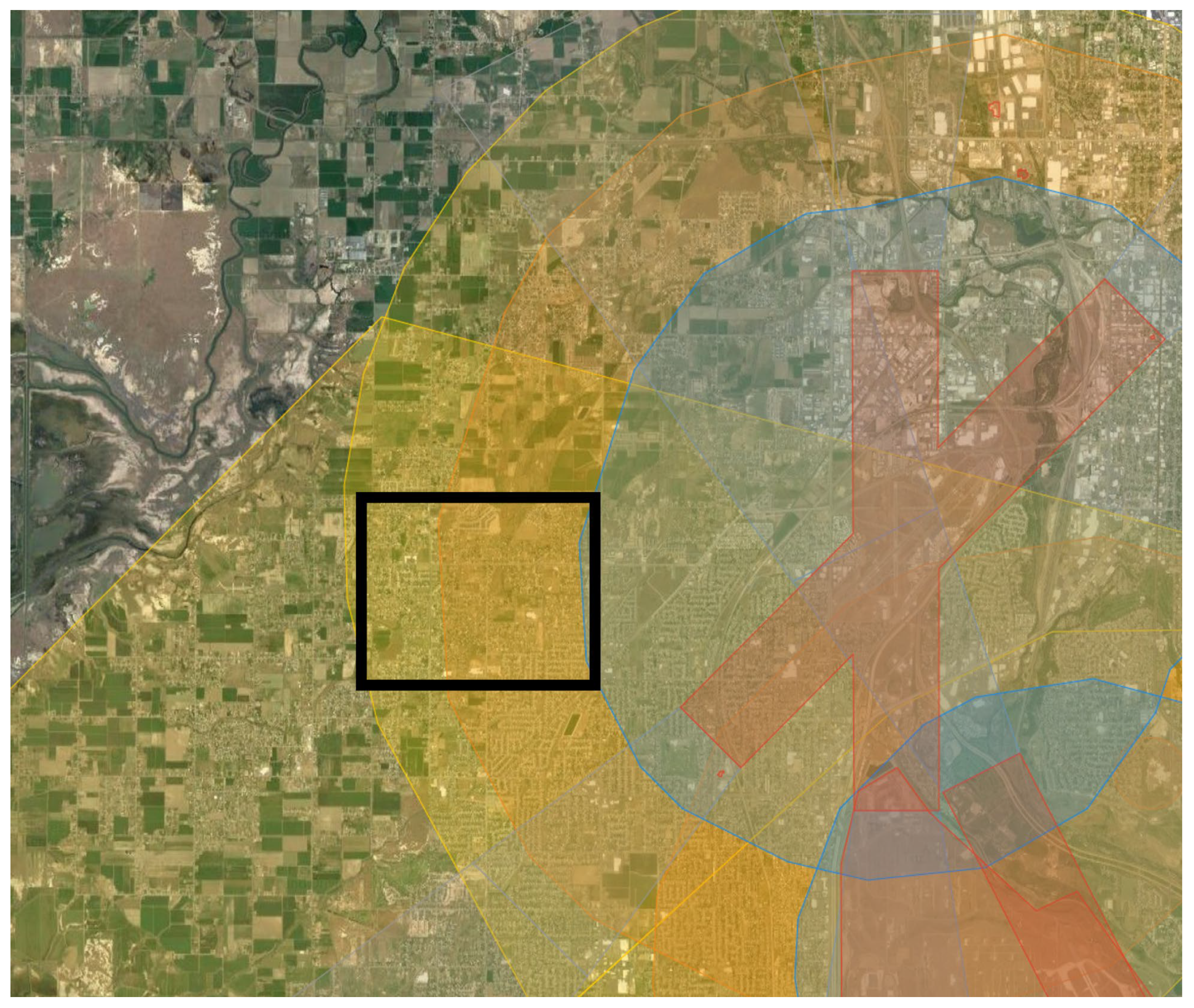
2.2. Study Area
2.3. Data
2.3.1. Aerial Imagery
2.3.2. Water Use Data
2.3.3. Evapotranspiration Data
2.4. Data Processing
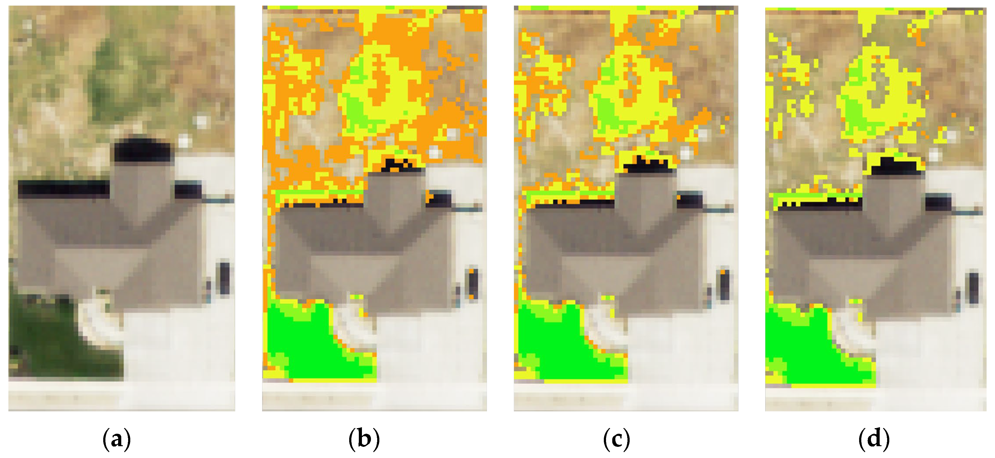
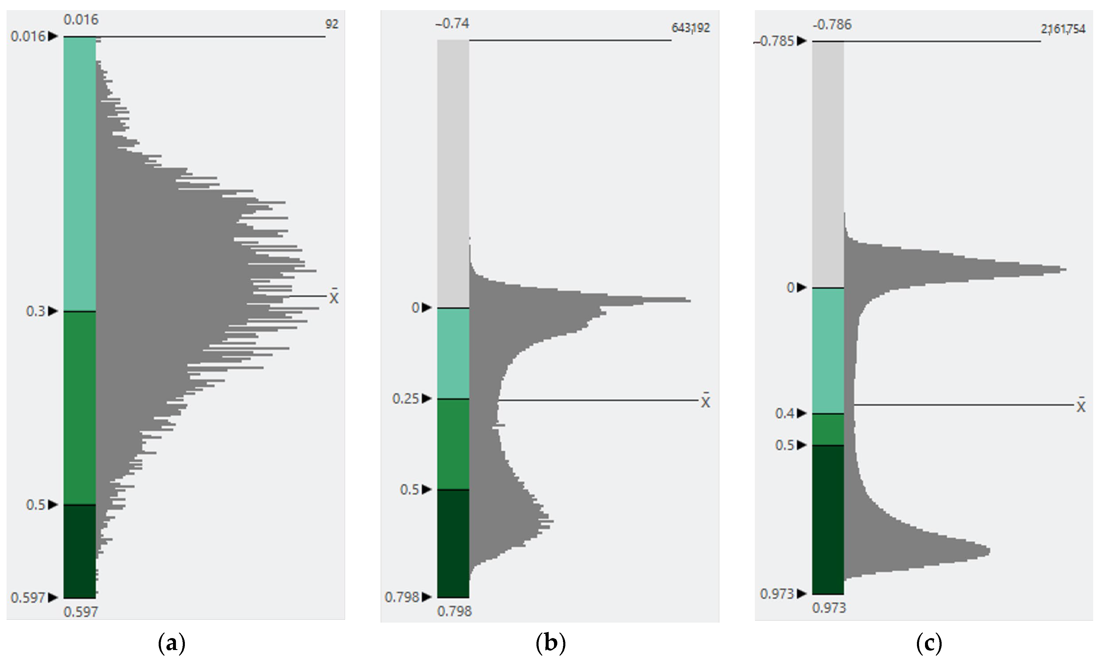
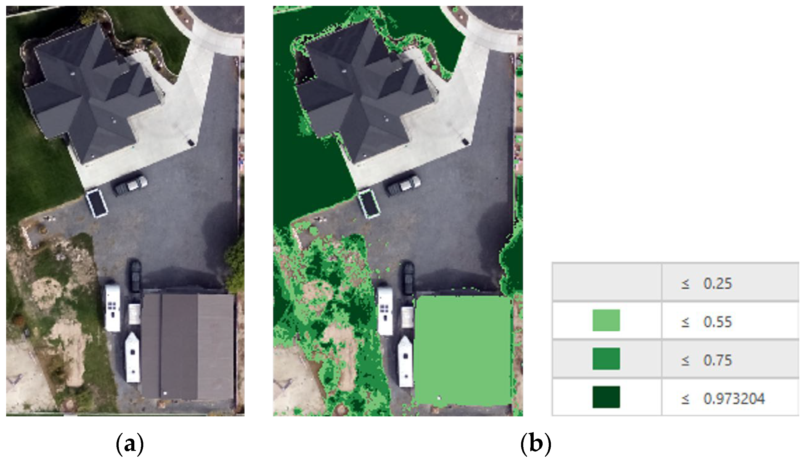
2.4.1. NDVI Threshold Selection
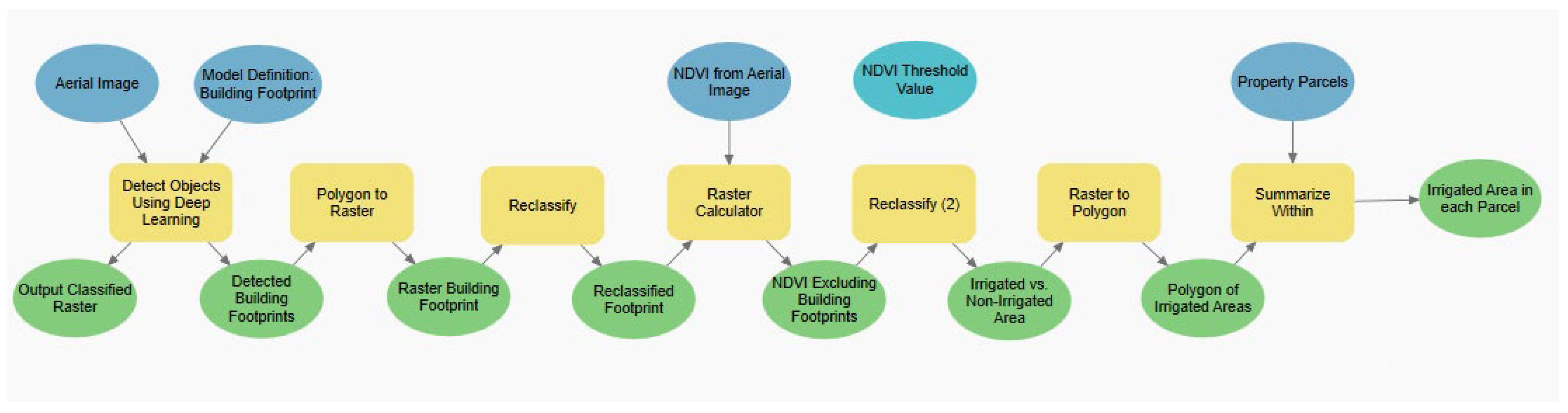
2.4.2. Quantifying Irrigated Area
2.4.3. Quantifying Irrigated Water Volume
3. Results
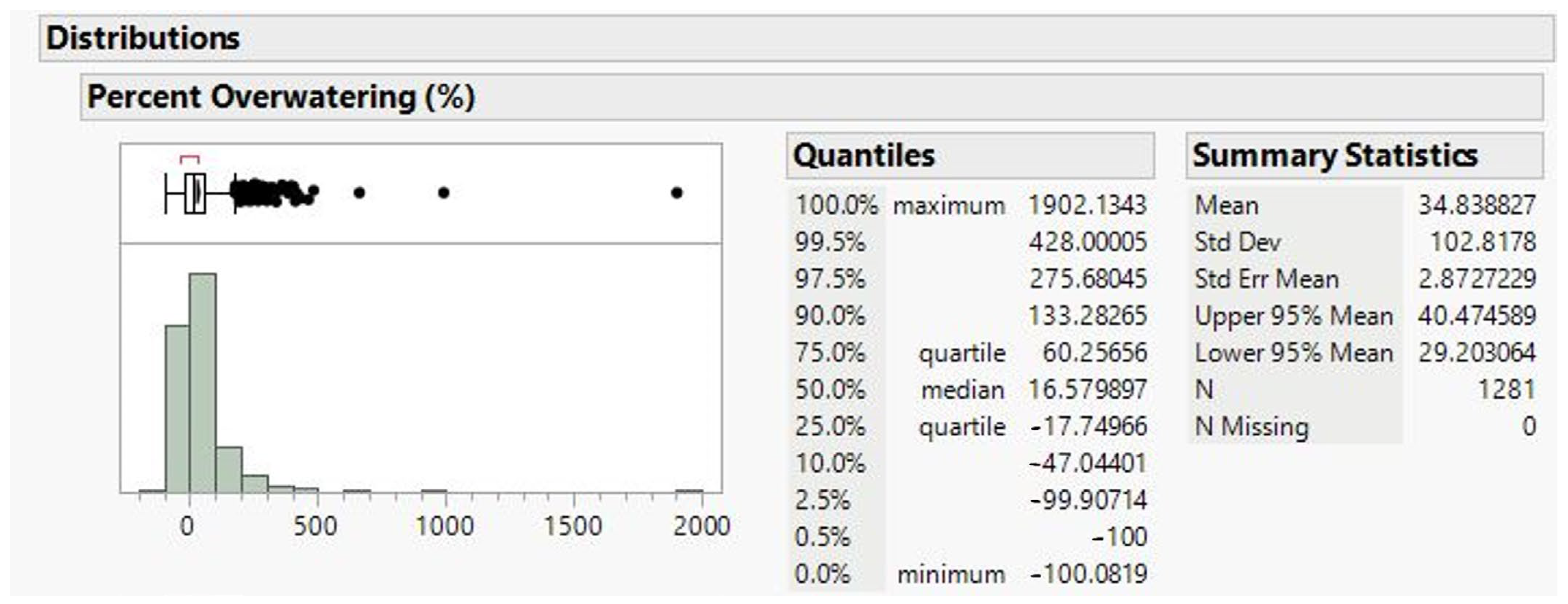
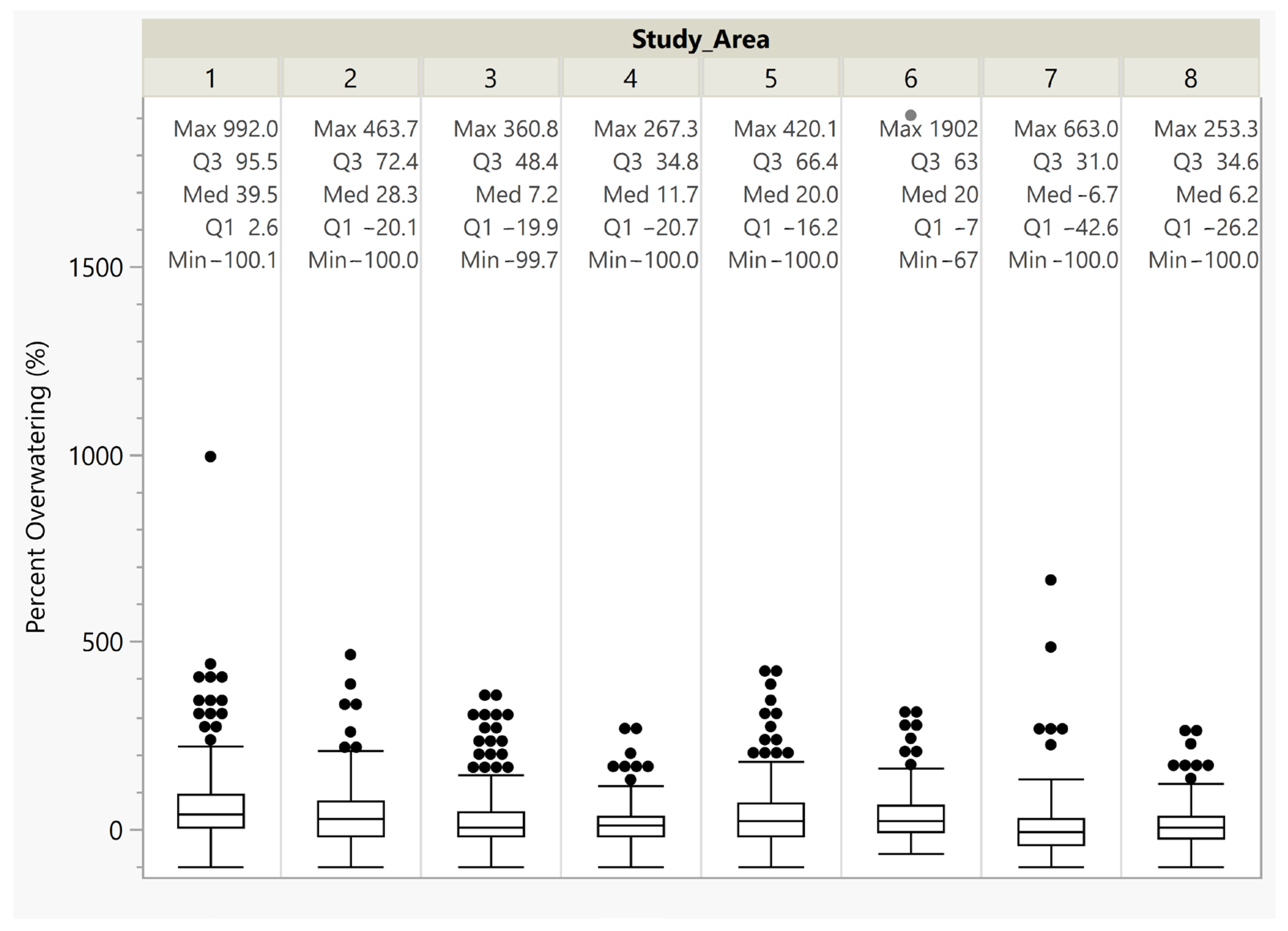
3.1. Data Outliers
3.2. Urban Irrigation Efficiency
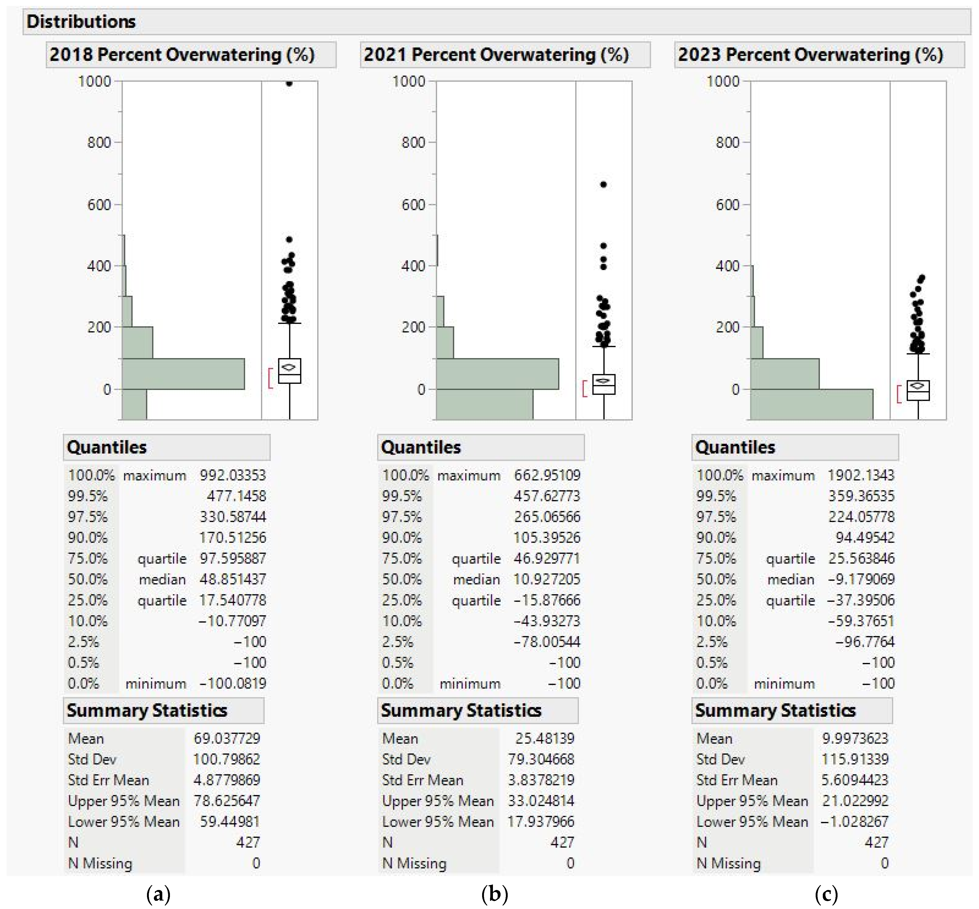
3.2.1. Year-to-Year Analysis
3.2.2. Lot Size Analysis
4. Discussion
4.1. Limitations
4.2. Recomendatations
5. Conclusions
Author Contributions
Funding
Institutional Review Board Statement
Informed Consent Statement
Data Availability Statement
Acknowledgments
Conflicts of Interest
References
- USGS. NDVI, the Foundation for Remote Sensing Phenology. Available online: https://www.usgs.gov/special-topics/remote-sensing-phenology/science/ndvi-foundation-remote-sensing-phenology#overview (accessed on 1 November 2022).
- Dieter, C.A.; Maupin, M.A.; Caldwell, R.R.; Harris, M.A.; Ivahnenko, T.I.; Lovelace, J.K.; Barber, N.L.; Linsey, K.S. Estimated Use of Water in the United States in 2015; U.S. Geological Survey: Reston, VA, USA, 2018. [Google Scholar] [CrossRef]
- Johnson, T.D.; Belitz, K. A remote sensing approach for estimating the location and rate of urban irrigation in semi-arid climates. J. Hydrol. 2012, 414–415, 86–98. [Google Scholar] [CrossRef]
- Shurtz, K.M.; Dicataldo, E.; Sowby, R.B.; Williams, G.P. Insights into Efficient Irrigation of Urban Landscapes: Analysis Using Remote Sensing, Parcel Data, Water Use, and Tiered Rates. Sustainability 2022, 14, 1427. [Google Scholar] [CrossRef]
- Sowby, R.B.; Lunstad, N.T. Why Is Residential Irrigation So Hard to Optimize? Water 2023, 15, 3177. [Google Scholar] [CrossRef]
- Hilaire, R.S.; Arnold, M.A.; Wilkerson, D.C.; Devitt, D.A.; Hurd, B.H.; Lesikar, B.J.; Lohr, V.I.; Martin, C.A.; McDonald, G.V.; Morris, R.L.; et al. Efficient Water Use in Residential Urban Landscapes. HortScience 2008, 43, 2081–2092. [Google Scholar] [CrossRef]
- Nouri, H.; Beecham, S.; Kazemi, F.; Hassanli, A.M. A review of ET measurement techniques for estimating the water requirements of urban landscape vegetation. Urban Water J. 2013, 10, 247–259. [Google Scholar] [CrossRef]
- Mini, C.; Hogue, T.S.; Pincetl, S. Estimation of residential outdoor water use in Los Angeles, California. Landsc. Urban Plan. 2014, 127, 124–135. [Google Scholar] [CrossRef]
- Salvador, R.; Bautista-Capetillo, C.; Playán, E. Irrigation performance in private urban landscapes: A study case in Zaragoza (Spain). Landsc. Urban Plan. 2011, 100, 302–311. [Google Scholar] [CrossRef]
- Harris, E. State and County Population Estimates for Utah: 2020. Inf. Decis. 2020. [Google Scholar]
- Sowby, R.B. Utah Is Not the Second-Driest State: A Lesson in Questioning Persistent Assumptions about Hydrology. J. Hydrol. Eng. 2024, 29, 02523001. [Google Scholar] [CrossRef]
- Utah Department of Natural Resources. Recent Updates (as of 11/30/23). Available online: https://drought.utah.gov/#:~:text=Last%20year%2090%25%20of%20the,year’s%2041%25%20at%20this%20time (accessed on 11 December 2023).
- Sanchez, M. Utah Water Conditions Update. 2023. Available online: https://water.utah.gov (accessed on 3 October 2024).
- Utah Department of Natural Resources. Slow the Flow. Available online: https://slowtheflow.org/ (accessed on 22 March 2024).
- Utah Legislature, H.B. 242—Secondary Water Metering Amendments. 2022. Available online: https://le.utah.gov/~2022/bills/static/HB0242.html (accessed on 23 October 2024).
- Capener, A.M.; Sowby, R.B.; Williams, G.P. Pathways to Enhancing Analysis of Irrigation by Remote Sensing (AIRS) in Urban Settings. Sustainability 2023, 15, 12676. [Google Scholar] [CrossRef]
- WeatherWX.com. Weber County Monthly Climate Averages. Available online: https://www.weatherwx.com/climate-averages/ut/weber+county.html (accessed on 2 November 2023).
- Huang, S.; Tang, L.; Hupy, J.P.; Wang, Y.; Shao, G. A commentary review on the use of normalized difference vegetation index (NDVI) in the era of popular remote sensing. J. For. Res. 2020, 32, 1–6. [Google Scholar] [CrossRef]
- USGS. USGS Earth Explorer. Available online: https://earthexplorer.usgs.gov/ (accessed on 12 September 2023).
- DJI. Fly Safe-GEO Zone Information. Available online: https://fly-safe.dji.com/nfz/nfz-query?zone=%5Bobject%20Object%5D&device=%5Bobject%20Object%5D (accessed on 13 November 2023).
- DJI. P4 Multispectral. Available online: https://www.dji.com/p4-multispectral (accessed on 22 March 2024).
- Utah Automated Geographic Reference Canter (AGRC). Utah Weber County Parcels LIR. Available online: https://opendata.gis.utah.gov/datasets/utah-weber-county-parcels-lir/explore?location=41.190846%2C-112.067093%2C-1.00 (accessed on 1 September 2023).
- Rodell, M.; Houser, P.R.; Jambor, U.; Gottschalck, J.; Mitchell, K.; Meng, C.J.; Arsenault, K.; Cosgrove, B.; Radakovich, J.; Bosilovich, M.; et al. The Global Land Data Assimilation System. Bull. Am. Meteorol. Soc. 2004, 85, 381–394. [Google Scholar] [CrossRef]
- OpenET. OpenET Data Explorer. Available online: https://explore.etdata.org/#5/39.665/-110.396 (accessed on 18 December 2023).
- Utah Climate Center. Network Overview. Available online: https://climate.usu.edu/mchd/dashboard/overview/USCAN.php (accessed on 11 January 2024).
- University of Idaho. Ref-ET Software. Available online: https://www.uidaho.edu/cals/kimberly-research-and-extension-center/research/water-resources/ref-et-software (accessed on 11 January 2024).
- Utah Climate Center. Eagle Lake. Available online: https://climate.usu.edu/mchd/dashboard/dashboard.php?network=AGWX&station=1231954&units=E&showgraph=0& (accessed on 11 January 2024).
- Mayer, P.W.; Deoreo, W.B. Improving urban irrigation efficiency by using weather-based “smart” controllers. J. AWWA 2010, 102, 86–97. [Google Scholar] [CrossRef]
- Zhang, L.; Sun, X.; Wu, T.; Zhang, H. An Analysis of Shadow Effects on Spectral Vegetation Indexes Using a Ground-Based Imaging Spectrometer. IEEE Geosci. Remote Sens. Lett. 2015, 12, 2188–2192. [Google Scholar] [CrossRef]
- Pepe, M.; Costantino, D.; Alfio, V.S.; Vozza, G.; Cartellino, E. A Novel Method Based on Deep Learning, GIS and Geomatics Software for Building a 3D City Model from VHR Satellite Stereo Imagery. ISPRS Int. J. Geo. Inf. 2021, 10, 697. [Google Scholar] [CrossRef]
- Lunstad, N.T.; Sowby, R.B. Smart Irrigation Controllers in Residential Applications and the Potential of Integrated Water Distribution Systems. J. Water Resour. Plan. Manag. 2024, 150, 03123002. [Google Scholar] [CrossRef]
- Utah Climate Center. Pleasant View-Thinnes Orchard. Available online: https://climate.usu.edu/mchd/dashboard/dashboard.php?network=FGNET&station=8&units=E&showgraph=0& (accessed on 22 March 2024).


| Year | Months | OpenET Actual (mm) | OpenET Reference (mm) | Reference ET (mm) |
|---|---|---|---|---|
| 2018 | July–August | 92.08 | 197.36 | 137.27 |
| 2021 | July–August | 89.28 | 195.07 | 170.08 |
| 2023 | August–September | 67.56 | 144.40 | 130.92 |
| Year | Adjusted Reference ET (mm) |
| 2018 | 164.72 |
| 2021 | 204.09 |
| 2023 | 157.11 |
| Image | NDVI Threshold |
|---|---|
| 2018 NAIP | 0.25 |
| 2021 NAIP | 0.20 |
| 2023 Drone Area 1 | 0.40 |
| 2023 Drone Area 2 | 0.27 |
| 2023 Drone Area 3 | 0.40 |
| 2023 Drone Area 4 | 0.15 |
| 2023 Drone Area 5 | 0.15 |
| 2023 Drone Area 6 | 0.19 |
| 2023 Drone Area 7 | 0.26 |
| 2023 Drone Area 8 | 0.23 |
| NDVI Threshold | Total Irrigated Area (m2) | Percent Variation from Original (%) |
|---|---|---|
| 0.20 | 754,206 | 5.84% |
| 0.23 | 727,500 | 2.09% |
| 0.25 | 712,580 | (original) |
| 0.27 | 697,754 | −2.08% |
| 0.30 | 675,089 | −5.26% |
| Median of Overwatering Amount (%) | Average of Overwatering Amount (%) | Average Percentage of Users Overwatering (%) |
|---|---|---|
| 16.6 | 34.8 | 64.4 |
| Year | Median Percentage Overwatering Amount (%) | Mean Percentage of Overwatering Amount (%) | Percentage of Users Overwatering (%) |
|---|---|---|---|
| 2018 | 48.9 | 69.0 | 87.5 |
| 2021 | 10.9 | 25.5 | 62.1 |
| 2023 | −9.2 | 10.0 | 43.7 |
Disclaimer/Publisher’s Note: The statements, opinions and data contained in all publications are solely those of the individual author(s) and contributor(s) and not of MDPI and/or the editor(s). MDPI and/or the editor(s) disclaim responsibility for any injury to people or property resulting from any ideas, methods, instructions or products referred to in the content. |
© 2024 by the authors. Licensee MDPI, Basel, Switzerland. This article is an open access article distributed under the terms and conditions of the Creative Commons Attribution (CC BY) license (https://creativecommons.org/licenses/by/4.0/).
Share and Cite
Turman, A.M.; Sowby, R.B.; Williams, G.P.; Hansen, N.C. Remote Sensing of Residential Landscape Irrigation in Weber County, Utah: Implications for Water Conservation, Image Analysis, and Drone Applications. Sustainability 2024, 16, 9356. https://doi.org/10.3390/su16219356
Turman AM, Sowby RB, Williams GP, Hansen NC. Remote Sensing of Residential Landscape Irrigation in Weber County, Utah: Implications for Water Conservation, Image Analysis, and Drone Applications. Sustainability. 2024; 16(21):9356. https://doi.org/10.3390/su16219356
Chicago/Turabian StyleTurman, Annelise M., Robert B. Sowby, Gustavious P. Williams, and Neil C. Hansen. 2024. "Remote Sensing of Residential Landscape Irrigation in Weber County, Utah: Implications for Water Conservation, Image Analysis, and Drone Applications" Sustainability 16, no. 21: 9356. https://doi.org/10.3390/su16219356
APA StyleTurman, A. M., Sowby, R. B., Williams, G. P., & Hansen, N. C. (2024). Remote Sensing of Residential Landscape Irrigation in Weber County, Utah: Implications for Water Conservation, Image Analysis, and Drone Applications. Sustainability, 16(21), 9356. https://doi.org/10.3390/su16219356