Exploring the Drivers of Soil Conservation Variation in the Source of Yellow River under Diverse Development Scenarios from a Geospatial Perspective

Abstract

Soil conservation (SC) plays a vital role in preventing soil erosion and ensuring ecological security. While current research on SC primarily focuses on historical spatiotemporal variations, there remains a dearth of sufficient simulation research exploring future development scenarios. In this study, simulations were applied to the source of Yellow River (SYR), a representative ecologically fragile area. Satellite remote sensing and product data, including precipitation, soil, land use/cover, DEM, and SPOT/VEGETATION NDVI, were utilized. The historical and future evolutionary trends of SC in the SYR were quantitatively assessed using the Revised Universal Soil Loss Equation (RUSLE) and trend analysis method, and the geographical detector was employed to explore the forces driving spatial differentiations in SC. The results demonstrated that: (1) 2000–2020, the spatial heterogeneity of SC in the SYR was characterized by the distribution of “gradually decreasing from Southeast to Northwest”, demonstrated a trend of “increasing, decreasing, and then increasing”. (2) Under the diverse development scenarios, the trend of SC change in the SYR was predominantly rising, and the natural change scenario (NCS) > ecological conservation scenario (ECS) > economic expansion scenario (EES). (3) Slope was the most important single driver affecting the spatiotemporal differentiation of SC, and the interaction of slope with average annual precipitation, and NDVI on the spatiotemporal heterogeneity of SC had the strongest explanatory ability. The results can serve as a scientific basis for regional SC and ecological protection and construction of the SYR.

1. Introduction

Soil conservation (SC) is a crucial ecosystem service that helps to prevent soil erosion and maintain regional ecological security [1,2,3]. Relevant research has indicated that the combined effects of human activities and climate change pose a global risk of significant reduction in SC capacity [4]. The escalating issue of soil loss not only leads to soil fertility degradation and decreased land productivity [2], but also negatively impacts habitat quality and biodiversity [2,5], as well as increases the likelihood of geological disasters and other security concerns [6,7]. These factors constitute a serious threat to the ecological security of countries and regions [8]. Consequently, enhancing the SC capacity of regional ecosystems and mitigating the impact of soil erosion have become focal points of international ecological conservation research and global sustainable development goals [8,9].

Soil erosion poses one of the greatest ecological challenges in China [10]. According to the 2020 China soil and water erosion communique, 1.12 × 10⁶ km² of region in China is disturbed by soil erosion, which has become one of the important factors restricting sustainable socio-economic development [11]. The source of Yellow River (SYR), located in the hinterland of the Qinghai-Tibet Plateau, serves as a crucial ecological security barrier in China and faces persistent issues with soil erosion [12]. The complex terrain and unique alpine geographical environment, coupled with warm and wet climate conditions, irregular precipitation patterns, and unsustainable human activities, distribute serious threats to soil security in the SYR [13]. Therefore, it is crucial to conduct a comprehensive and scientific evaluation of spatiotemporal changes and driving factors related to SC service functions in the SYR. This evaluation will play a vital role in safeguarding the ecological security of the SYR and promoting sustainable development in the semi-arid zone.

With the continuous development of geographic information system (GIS) and remote sensing (RS) technologies, they have been widely applied in the field of ecological environment monitoring. GIS enables spatial information analysis and processing, allowing for spatiotemporal analysis of ecosystem processes with high spatial integration and dynamic prediction capabilities. And RS is a spatially insensitive detection technique that can acquire high spatiotemporal resolution images with wide coverage. Currently, relevant studies combine the image analysis techniques of RS with the spatial analysis capabilities of GIS to assess regional SC by obtaining and analyzing high-resolution RS images. This approach is applied to evaluate the impact of vegetation coverage on SC [14,15], detect the distribution and changes of SC and sedimentation [16,17], analyze the spatiotemporal correlation between SC and other environmental factors [18,19], and identify the influencing factors of SC such as precipitation, slope, and land use changes [20,21].

Current SC research primarily employs two methods: physical process-based measurements and empirically based statistical models [22,23]. The physical process-based measurement methods, including isotope tracer [24] and regional monitoring method [25], offer high precision at sample scale and maintain obvious advantages in soil erosion mechanism research. However, due to the complexity of the measurement work and the challenge of reflecting regional-scale situations, these methods have limitations in soil erosion assessment [26]. Besides, empirically based statistical models evaluate regional-scale soil erosion conditions by establishing statistical relationships between soil erosion and RS image pixel values. Due to the variances in electromagnetic wave reflection characteristics caused by diverse land features and environmental changes, alterations in soil erosion within a particular region will correspondingly induce variations in the reflectance of the corresponding areas in remote sensing imagery. Empirically based statistical models have been widely used in large-scale SC research [27], especially the Revised Universal Soil Loss Equation (RUSLE) [2,28]. Due to the high applicability and stability, RUSLE has been applied to the studies on the spatiotemporal variability characteristics of SC in watersheds [29,30], the sensitivity of SC to diverse erosivity factors [31], and the diverse spatial scales of soil loss estimation [32]. In China, RUSLE has been extensively applied in SC studies in diverse regions, including the Qinghai-Tibet Plateau [33], the Loess Plateau Basin [34], the Chaohu Basin [35], the Karst region [27], and the Three Gorges region [36], leading to improved assessment results. However, these studies overlook the further evaluation of the driving effects between SC services and the contributing factors.

Previous studies have highlighted that soil mobility is dominantly influenced by natural geographical conditions (such as climate, landform, and vegetation) and human interventions [8]. The impact of these factors varies across diverse regions [8,13,37]. Consequently, a better understanding of the relationship between SC services and driving factors is crucial for effective management and development of SC measures. Current models for exploring the driver can be categorized into non-spatial and spatial models [38]. Non-spatial models predominantly involve stepwise regression analysis [39] and the ordinary least square method [40]. However, these models are limited in explaining the effects of drivers in two dimensions. The spatial models, such as geographical detector (GD) [41], and the geographically weighted regression [42] take into account spatial variability in the potential effects of the drivers, leading to more accurate assessment results [43]. Among the spatial model, the GD offers unique advantages in analyzing the coupling effects between drivers and driving factors, resulting in relevant studies applied to the analysis of soil erosion drivers in diverse landscapes during historical periods [10,44,45]. However, none of the existing studies have explored the future driving effects on SC to provide insights for regional SC in a precautionary manner.

Considering the existing conditions and problems, this study aims to investigate the evolutionary trend of SC services in the SYR over the past and under diverse development scenarios (DDS), analyzing the drivers behind the phenomenon and the interactions between these drivers. The study aims to provide decision-makers with a reference for future SC protection in the SYR and offer ideas for regional ecological preservation. The primary objectives are as follows: (1) to quantify the spatial distribution of SC in the SYR from 2000 to 2020, (2) to simulate the SC under the DDS from 2021 to 2030, (3) to evaluate the trend of spatiotemporal evolution of the SC, and (4) to explore the key drivers that significantly impact SC.

2. Materials and Methods

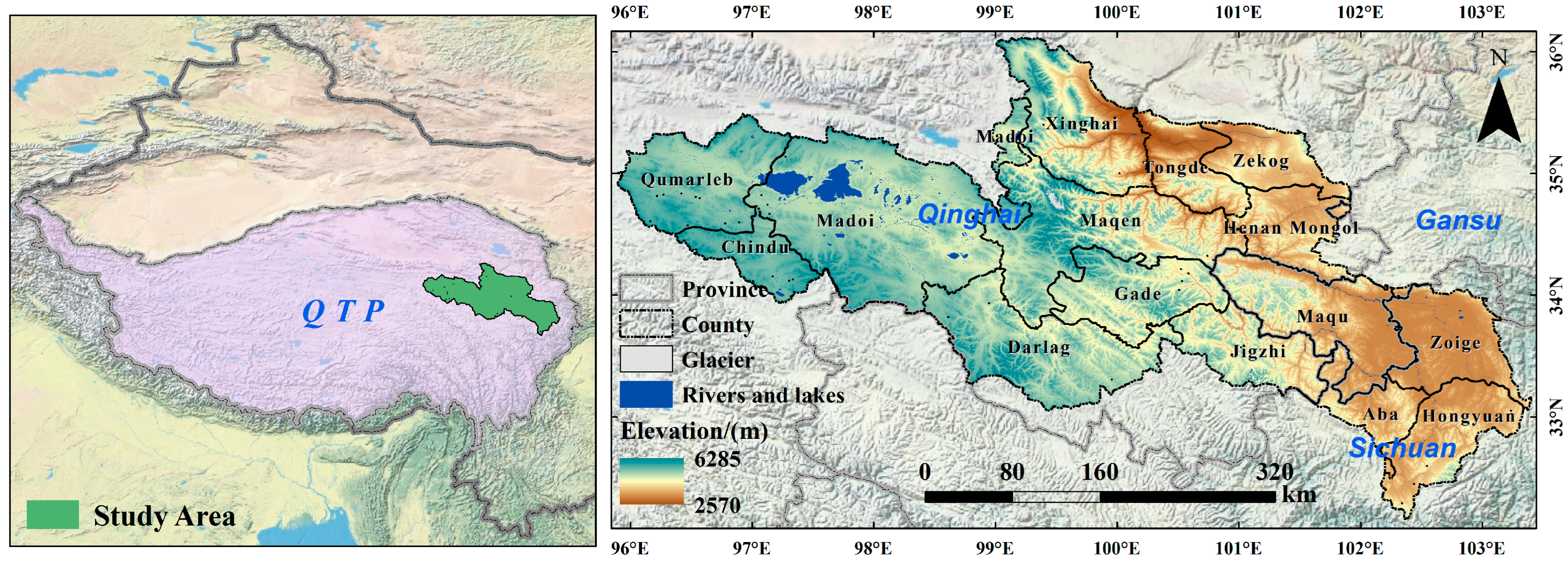
2.1. Study Area

The SYR (95°52′–103°25′ E, 32°30′–36°34′ N, Figure 1), located in the northeast of the Qinghai-Tibetan Plateau (QTP), with crisscrossing water systems and widespread grasslands, has the reputation of “Yellow River Water Tower” [46]. The region encompasses six states and eighteen counties, where the provinces of Qinghai, Sichuan, and Gansu converge, including a watershed of approximately 1.23 × 10⁵ km² upstream of Tangnaihai hydrologic station in the Yellow River Basin [47]. The topography of the SYR declines from west to east, with an average elevation of approximately 4000 m, covered with mountains, basins, canyons, grasslands, and swamps [48]. Alpine grasslands are vastly distributed in the region, dominated by land use/cover (LUC) types such as alpine grasslands, alpine meadows, alpine scrubs, and marshes [48,49]. Additionally, the SYR is part of the semi-arid zone of China, belonging to the typical plateau continental climate. The region experiences alternating periods of heat and cold, accompanied by distinct humid and dry seasons. It benefits from abundant moisture, with average annual precipitation ranging from 220 to 780 mm. [50]. Due to its delicate ecological environment, the SYR is highly vulnerable to climate and environmental fluctuations. Consequently, conducting a comprehensive scientific investigation into the ecosystem services under the DDS in the SYR is crucial for ecological protection and construction.

2.2. Datasets and Processing

The major data used for this study included meteorological, vegetation, geomorphology, and environmental data. Specific information is shown in

Table 1. Description of the data.

Type	Data	Period	Spatial Resolution	Sources
Meteorological	Precipitation (0.1 mm)	2000~2020	1 km	Loess Plateau Science Data Center (LPSDC), National Earth System Science Data Sharing Infrastructure (NESSDSI), and National Science & Technology Infrastructure of China (NSTIC) (LNN, http://loess.geodata.cn (accessed on 18 April 2023))
		2021~2030	1 km	LNN (http://loess.geodata.cn (accessed on 18 April 2023))
Vegetation	LUC	2000, 2010, and 2020	30 m	Resource and Environmental Science and Data Center (RESDC) of the Chinese Academy of Sciences (http://www.resdc.cn (accessed on 20 April 2023))
	NDVI	2000~2020	1 km	RESDC (http://www.resdc.cn (accessed on 20 April 2023))
		2021~2030	1 km	Processed
Geomorphology	DEM	2009	30 m	Geospatial data cloud (http://www.gscloud.cn (accessed on 18 April 2023))
	Soil type	1995	1 km	Chinese soil dataset (v1.1) of the Big Data of Science in Cold and Arid Regions (http://westdc.westgis.ac.cn (accessed on 19 April 2023))
Environmental	Water	2005	30 m	RESDC (http://www.resdc.cn (accessed on 19 April 2023))
	Boundary	2015	——	RESDC (http://www.resdc.cn (accessed on 19 April 2023))

. To evaluate the past and simulate the DDS of SC, the historical and future periods of precipitation data employed in this study, including 2000~2020 and 2021~2030 for SSP119, SSP245, and SSP585 scenarios, respectively, based on the global 0.5° climate dataset released by Climatic Research Unit (https://crudata.uea.ac.uk/cru/data/hrg/ (accessed on 18 April 2023)) and the global > 100 km climate model dataset released by the IPCC (intergovernmental panel on climate change) were coupled with model intercomparison programme phase 6 (CMIP6, https://www.wcrp-climate.org/wgcm-cmip/wgcm-cmip6 (accessed on 18 April 2023)), and the high-resolution climate dataset released by WorldClim (http://www.worldclim.org/ (accessed on 18 April 2023)), generated by the delta spatial downscaling scheme for regional downscaling in China region. Additionally, this study extracted soil type, soil sand, silt, clay, and soil organic carbon content from the soil data, and reclassified the LUC data according to the Chinese LUC classification method proposed in previous research [51], combined with the actual vegetation cover in the SYR (Reclassification as shown in

Table 2. LUC classification and its ecological level in the SYR.

This Study		LUC Classification System of RESDC
Level	LUC *	Class 1	Class 2
1	WTL	4 Wetland	41 River
			42 Lake
			43 Reservoir pit
			44 Snow
			45 Mudflats
			46 Shoal
			64 Marshland
2	WL	2 Woodland	21 Woodland
			23 Sparse woodland
			24 Other woodland
3	S	2 Woodland	22 Shrub
4	HCG	3 Grassland	31 High coverage grassland
5	MCG	3 Grassland	32 Moderate coverage grassland
6	LCG	3 Grassland	33 Low coverage grassland
7	BL	6 Unused land	61 Sandy land
			62 Desert
			63 Saline soil
			65 Bare grounds
			66 Bare rocks
8	FL	1 Farmland	11 Paddy field
			12 Arid lands
9	CL	5 Construction land	51 Townland
			52 Rural settlements
			53 Other construction land

* WTL: Wetland, WL: Woodland, S: Shrub, HCG: High coverage grassland, MCG: Moderate coverage grassland, LCG: Low coverage grassland, BL: Bare land, FL: Farmland, CL: Construction land, LUC: land use/land cover type, RESDC: Resource and Environmental Science and Data Center.

). To facilitate the analysis, the spatial resolution of the data used in this study will be uniformly resampled to 100 m, and the projection coordinates were unified as the GCS_WGS_1984 projection.

2.3. Research Methodology

Changes in precipitation and LUC can exert both direct and indirect influences on SC by regional ecosystems. Therefore, exploring the response of SC to precipitation and LUC changes (LUCC) under the DDS contributes to the establishment of appropriate SC measures. In this study, we constructed a SC research framework based on the RUSLE-GD model. The RUSLE model was employed to evaluate the SC from 2000 to 2020 and under DDS from 2020 to 2030, and the GD model was utilized to explore the driving effects of diverse drivers on SC (Figure 2).

2.3.1. Scenario Design for SC Variations

To reveal the characteristics of LUCC under the DDS, three scenarios were designed: the natural change scenario (NCS), the ecological conservation scenario (ECS), and the economic expansion scenario (EES). The NCS represents a development scenario that continues to follow historical trends, with the rate of vegetation cover change remaining consistent with the period of 2000–2020. The ECS prioritizes the prioritization of the protection of ecological land, resulting in an increase in vegetation cover, and the EES prioritizes economic development, with a decrease in vegetation cover. Further details are depicted in

Table 3. Scenario design.

Scenario	Design Content
NCS	The NCS continues the trend of 2000–2020, wherein 2021–2030 NDVI is computed year by year by linear regression from 2000–2020. The precipitation data of future scenario SSP245 was adopted.
ECS	Since the vegetation growth trend is slightly higher in the ECS than in the NCS, the NDVI from 2021 to 2030 in the NCS is increased by 10%. The precipitation data of future scenario SSP119 was used.
EES	The EES is biased towards economic development, and the vegetation growth trend under this scenario is lower than the NCS; hence, it is reduced by 10% from the NCS 2021–2030 NDVI. And the precipitation data of future scenario SSP585 was used.

.

2.3.2. Land Cover Change Index (LCCI)

In this study, the LCCI [52] was utilized to assess the magnitude of LUCC during a specific period. According to the ecological contribution of diverse LUC types and taking the changes in ecological integrated functions before and after LUCC, nine LUC types in the SYR were classified into ecological levels (Table 2). A rank of 1 indicates a higher ecological integrated function for a particular LUC type. When LUCC occurs, a difference in rank is observed. A positive difference value indicates an improvement in the ecosystem, while a negative value reflects degradation caused by LUC. The specific computation formula is as follows:

$$LCCI=\frac{{\displaystyle {\sum }_{k=1}^9\left[A_k\times \left(D_a-D_b\right)\right]}}{A}\times 100\%$$

(1)

When LCCI is positive, it indicates that the regional LUC and macro-ecological status has improved, otherwise it indicates that degradation has occurred. k = 1, 2, ......, 9, for the LUC type, A_k is the area where k has changed, and A is the total area of the analyzed region. D_a and D_b denote the ecological levels of LUC before and after the occurrence of LUC, respectively.

2.3.3. Quantization of SC

In this study, diverse natural climatic conditions of the region are referred to and comprehensively considered in the computations. Since factors K and LS are determined by soil texture structure, distribution, and landform, their differences in time series can be ignored.

SC denotes the margin between potential (A_p) and actual soil erosion (A_r) that would occur on land in the absence of vegetation cover and human management conditions. In this study, SC is computed based on the RUSLE [53] model:

$$SC=A_p-A_r=R\times K\times LS\times \left(1-C\times P\right)$$

(2)

where SC denotes the soil conservation value (t/(km²·a), 0.01 t/(hm²·a) = 1 t/(km²·a)), R means the precipitation erosion factor (MJ·mm/(hm²·h·a)), K denotes the soil erodibility factor (t·ha·h/(hm²·MJ·mm)), LS denotes the topographic factor (L represents the slope length factor and S denotes the steepness factor), C reflects the vegetation cover and management factor, P denotes the soil and water conservation measures factor.

R represents the kinetic criterion for soil erosion caused by runoff from precipitation, while the intensity and duration of rainfall have a significant effect on erosion. R is computed by the Wischmeier empirical formula [54]:

$$R={\displaystyle {\sum }_{i=1}^{12}\left(1.735\times {10}^{1.5{\log }_{10}\left(\frac{p_i^2}{p}\right)-0.8188}\right)}$$

(3)

where p_i denotes the monthly precipitation (mm) and p reflects the average annual precipitation (mm).

K reflects the sensitivity of soil to the separation and transport of erosion forces, with coefficients ranging from 0 to 1. The soil erosion sediment module of the Erosion Productivity Impact Calculator (EPIC) model proposed by previous research [55] was used:

$$\begin{array}{l}K=\left\{0.2+0.3\exp (-0.0256San(1-\frac{Sil}{100}))\right\}\times \left(\frac{Sil}{Cal+Sil}\right)\times \left[1-\frac{0.25TOC}{TOC+\exp (3.72-2.95TOC)}\right]\times \left[1-\frac{0.7SN}{SN+\exp (-5.51+22.9SN)}\right]\times 0.1317\\ SN=1-\frac{San}{100}\end{array}$$

(4)

where San, Sil, Cal, and TOC respectively refer to sand, silt, clay, and soil organic carbon content (%), and 0.1317 is the international unit conversion factor.

LS is the contribution of topographic and geomorphological feature on soil loss. In this study, DEM data with 30 m resolution and the factor computation program developed by Arc Marco Language (AML) by previous research [56] were used on the Arc Info workstation.

C denotes the role of vegetation cover and management practices on soil loss. In this study, the method developed by previous research [57] using NDVI and NOAA AVHRR remote sensing data was used and the parameters α and β were set to 2.5 and 1, respectively, to compute the factor:

$$C=\exp \left(-\alpha \cdot \frac{NDVI}{\beta -NDVI}\right)$$

(5)

P denotes the ratio of soil loss under a particular soil and water protection management to soil erosion when planted downslope, with values in the range of 0 to 1, where 0 means that no erosion occurs after the implementation, while 1 for failure to implement appropriate soil and water conservation measures. The value was obtained by referring to the relevant literature, and the specific parameters as depicted in

Table 4. The p value for the LUC.

LUC	FL	WL	HCG	MCG	LCG	WTL	CL	S	BL
p	0.5	0.4	0.7	0.7	0.7	0.2	0.5	0.4	1

.

2.3.4. Detection of SC Dynamic Changes

To investigate the trend of SC in the SYR from 2000 to 2020, the Theil-Sen Median trend analysis method (TSM) with Mann-Kendall test (MKT) was used [58,59]. The TSM was used to evaluate the dynamic variation trend from 2000 to 2020, with time as the independent variable and SC as the dependent variable. The analysis is computed according to:

$$S_{SC}=Median\left(\frac{S{C}_i-S{C}_j}{j-i}\right),\begin{array}{cc}& \end{array}\forall 1<i<j,$$

(6)

where S_SC represents the Theil-Sen median, SC_j and SC_i, respectively, denote the SC in the year of j and i. If S_SC is positive, then the variable consistently increases in time, a negative value of S_SC means decrease.

The MKT was used for testing the significance of trend in SC, computed as follows:

$$\begin{array}{c}S={\displaystyle {\sum }_{i=1}^{n-1}{\displaystyle {\sum }_{j=i+1}^{n}sign(S{C}_j-S{C}_i)}}\\ Z=\left\{\begin{array}{c}\frac{S-1}{\sqrt{\mathrm{var}(S)}}\begin{array}{ccc}& & \end{array}S>0\\ 0\begin{array}{ccccc}& & & & \end{array}S=0\\ \frac{S+1}{\sqrt{\mathrm{var}(S)}}\begin{array}{ccc}& & \end{array}S<0\end{array}\right.\end{array},$$

(7)

where n is the length of the cycle from i to j, SC_i and SC_j, respectively, denote the SC corresponding to time series i and j (i < j), sign() is the sign function. The computed Z value is the standardized test statistic, and Z_(1-α/2) is the value corresponding to the confidence level α. In this study, the significance of the trend of SC is discussed at the confidence levels of α = 0.05 and α = 0.01, and the trend results as depicted in

Table 5. Classification of the SC trend inspection in the SYR.

α	SSC	Z	SC Trend
0.01	>0	|Z| > 2.58	Significantly increase
0.05	>0	2.58 > |Z| > 1.96	Slightly increase
0.05	>0/<0	|Z| < 1.96	No significant change
0.05	<0	2.58 > |Z| > 1.96	Slightly decrease
0.01	<0	|Z| > 2.58	Significantly decrease

.

2.3.5. Geographical Detector (GD)

GD is a geostatistical method employed to characterize the spatial differentiation of geographic processes and to explore differences in the drivers behind the representations [41]. In this study, the factor, the interaction, and the risk detector were applied to characterize the contribution of diverse drivers to the spatial heterogeneity of SC under the DDS. The factor detector was employed to explore the spatial heterogeneity of SC, and to reflect the explanatory ability of each driving factor for differences in the spatial heterogeneity of SC, which is computed as follows:

$$\mathrm{q}=1-\frac{{\displaystyle {\sum }_{h=1}^L{N}_h{\sigma }_h^2}}{N{\sigma }^2}$$

(8)

where q denotes the explanatory ability of an explanatory factor X for the explained factor Y (SC), and ranges from 0 to 1. A higher q value indicates stronger explanatory ability of the factor X for SC spatial heterogeneity. N and σ², respectively, are the number of samples and the variance of the indicator. And h ranges from 1 to L and represents the number of factors grading layers (including classification or partitioning). In this study, NDVI, annual precipitation, DEM, slope, soil type, and LCCI were selected as the driving factors. The annual precipitation, DEM, slope, and LCCI were discretized and homogenized into nine grades by the natural breakpoint method, including the soil type which was classified into ten types (respectively: black calcareous, black felted, meadow, grass felted, peat, swampy, chilled calcareous, chilled primeval, chilled permafrost, and primrose soil) based on soil properties.

Subsequently, the interaction detector was employed to characterize the interactions between diverse drivers, i.e., to evaluate whether the combined contribution of two variables (as X1 with X2) increases or decreases the explanatory ability of the spatial heterogeneity of SC. Specifically, the assessment is based on computing the q value (q(X1) with q(X2)) of single factor X1 and X2 for dependent variable Y, respectively, and the interaction index (q(X1∩X2)) resulting from overlay (or interaction). The risk detector was employed to explore whether there is a significant difference between subintervals of the two factors (X1, X2) affecting SC, and the t statistic was applied to test whether the driving force of the drivers was statistically significant at 95% significance level.

3. Results

3.1. SC Spatiotemporal Variations

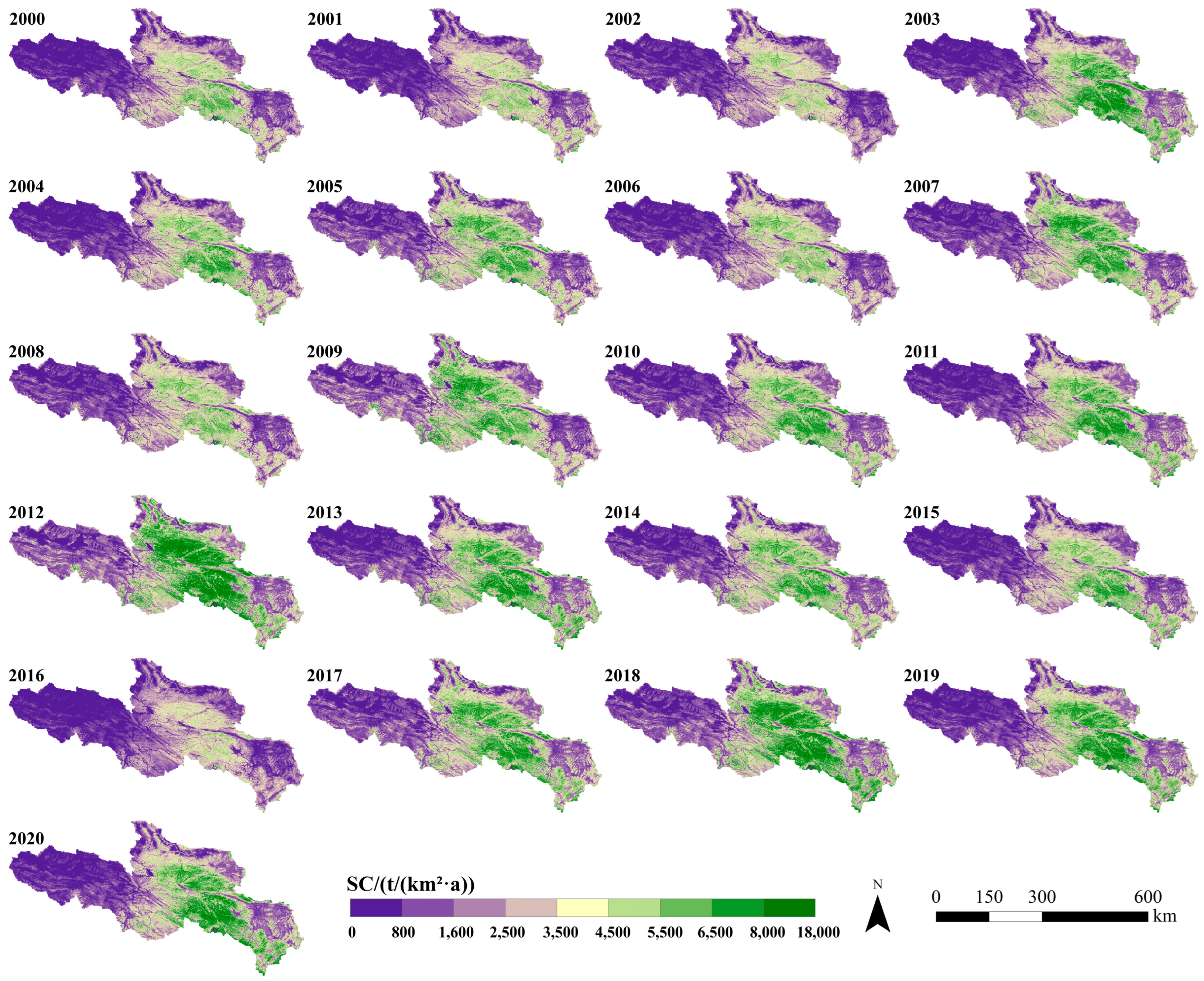
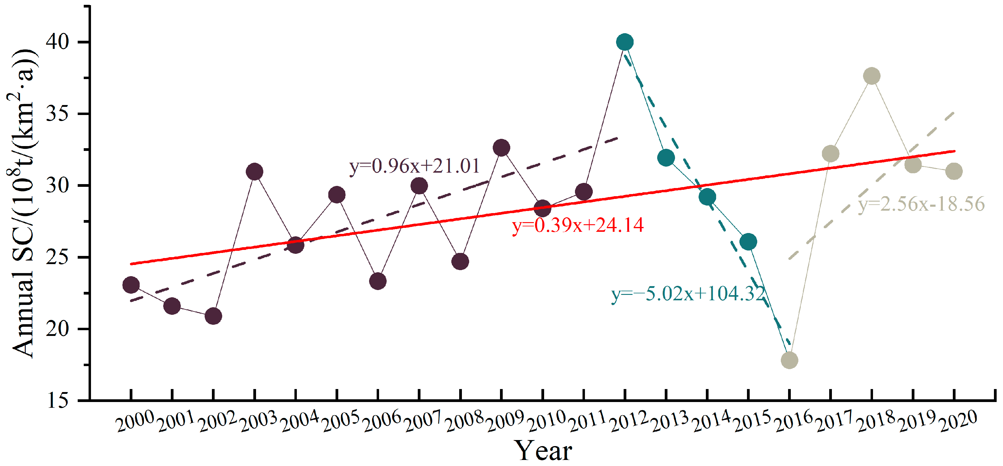
3.1.1. SC Spatiotemporal Changes in 2000 to 2020

The spatial heterogeneity of SC services in the SYR was characterized by a gradual decrease from southeast to northwest. The south-central part of the SYR exhibited predominantly high SC values, while the northwestern part had lower SC values (Figure 3). Jigzhi county, located in the south of the SYR, maintained the highest average SC of 5654.75 t/(km²·a). Aba, Gade, Maqu, Maqen, and Henan Mongol counties had average SC values greater than 3500 t/(km²·a). Besides, Qumarleb, Madoi, Chindu, and Zoige counties were characterized by poor SC, with average values below 2000 t/(km²·a), and Qumarleb county had the lowest average SC of approximately 796.04 t/(km²·a). The average annual SC in the SYR from 2000 to 2020 was 2918.35 t/(km²·a), with regions above this average level accounting for 53.18% of the SYR.

From 2000 to 2020, the average annual SC in the SYR exhibited a fluctuating upward trend, divided into three stages of increase, decrease, and subsequent increase (Figure 4). In terms of interannual changes, the first stage (2000–2012) showed a more pronounced enhancement in SC, with an increase of 42.30%, equivalent to 16.92 × 10⁸ t/(km²·a). The second stage (2012–2016) witnessed a drastic reduction, with a decrease of 22.18 × 10⁸ t/(km²·a), corresponding to a 55.45% decrease. The third stage (2016–2020) exhibited a greater enhancement compared to the first stage, with a 73.91% increase from 17.82 × 10⁸ t/(km²·a) in 2016 to 30.99 × 10⁸ t/(km²·a) in 2020. Overall, the SC in the SYR increased by 34.27% from 23.08 × 10⁸ t/(km²·a) in 2000 to 30.99 × 10⁸ t/(km²·a) in 2020 over the two decades.

Additionally, the spatial distribution of SC variation trends in the SYR from 2000 to 2020 was dominated by an increase (Figure 5). Approximately 90% of the total area in the SYR maintained a trend towards SC growth. The central part of the SYR was the dominant area with a significant increase in SC, while the largest region with an insignificant increase was mostly distributed in the southeast and west of the SYR. However, an insignificant reduction trend in SC was observed in Qumarleb county in the northwest of the SYR.

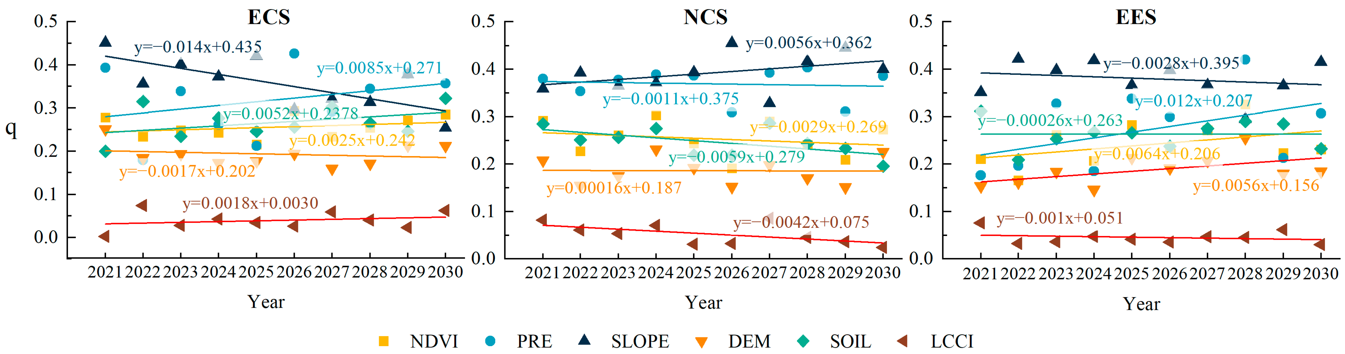
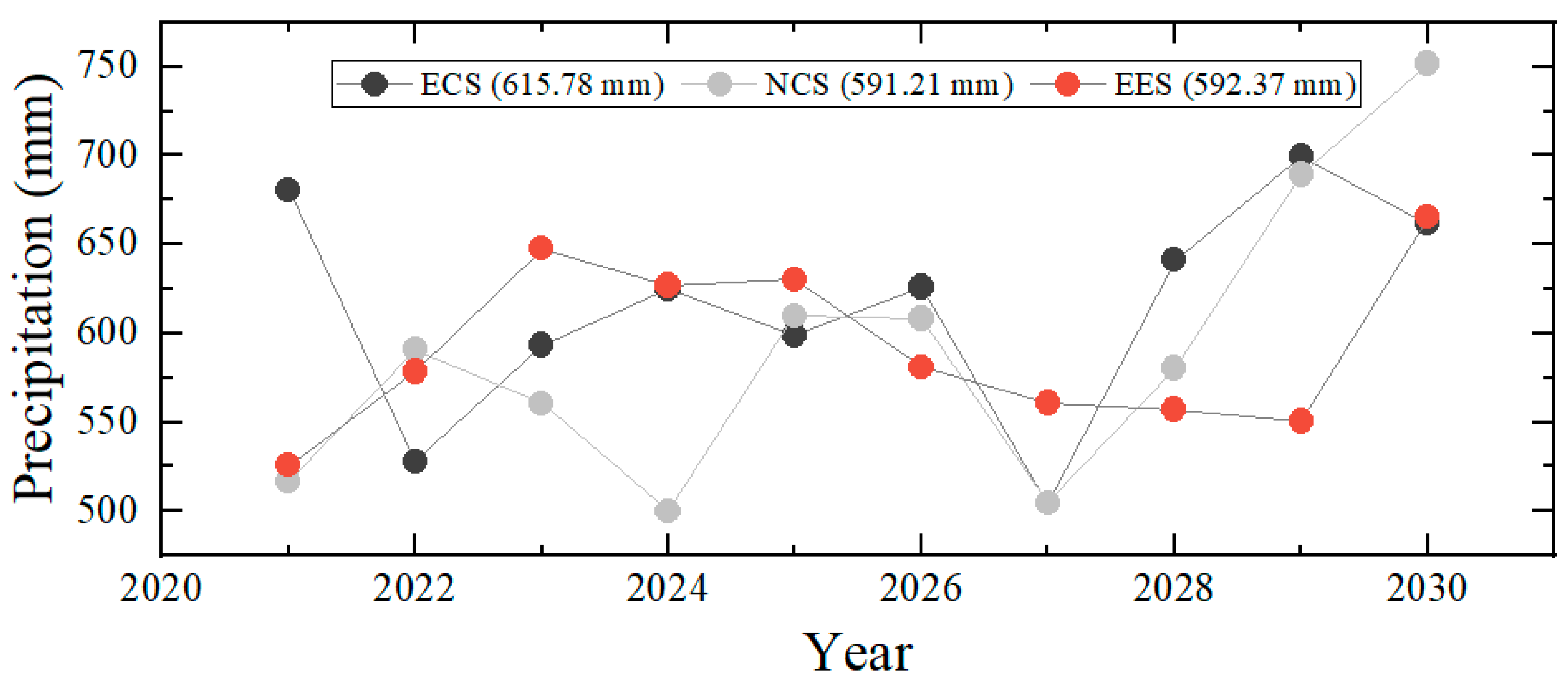
3.1.2. The Simulations of SC and Its Changes in 2021–2030

The trends of SC services change under the DDS, and annual estimates for the SYR from 2021 to 2030 revealed considerable variations in the spatiotemporal trends of SC under the DDS (Figure 6). In the ECS, regions with increasing and decreasing trends in SC accounted for 80.24 and 5.86% of the total area of the SYR, respectively. The areas with a significant increase were primarily located in the east-center region of the SYR, while regions with an insignificant increase were distributed in the west. Areas with no significant change and insignificant reduction were located in the southeast and south-center parts of the SYR. Under the NCS, 33.92% of the SYR exhibited a significant increase trend in SC with a concentrated distribution in the center, north, and northwest. Meanwhile, 4.59% of the SYR demonstrated an insignificant reduction trend in SC, primarily distributed in the southeast. In the EES, areas demonstrating an increase trend in SC were distributed in the north-center part of the SYR, accounting for 76.43% of the area of the source. The regions with a significant increase in SC accounted for 19.64% of the area, while the regions with insignificant reduction and no significant change in SC were predominantly distributed in the southeast and south of the SYR. Overall, the variation trends in SC under the DDS indicated a similar distribution, with a significant increase in the center and an insignificant reduction in the southeast. Moreover, the order of the significant increase rate of SC under the DDS was NCS (33.92%) > ECS (21.08%) > EES (19.64%).

Regarding interannual variations (see column statistics and linear regression plots in Figure 6), the SC services exhibited diverse levels of increase under the DDS. The ECS and NCS showed a similar growth trend, with the SC change in the NCS slightly smaller than that of the ECS. Compared to the total SC in 2020 (30.99 × 10⁸ t/(km²·a), the SC in the ECS increased by 23.32 × 10⁸ t/(km²·a) over the next ten years, accounting for a 75.26% increase. Similarly, the SC under the NCS increased by 21.92 × 10⁸ t/(km²·a), reflecting an increase of 70.72%. In contrast, the SC of the EES exhibited a steady increase trend with weak interannual variability, resulting in an incremental increase of 18.57 × 10⁸ t/(km²·a) by 2030, representing an increase of about 60%. In conclusion, the largest growth trend of SC in the SYR from 2021 to 2030 was observed under the NCS, followed by the ECS, while the EES exhibited the smallest growth.

3.2. The Drivers of Spatial Variability in SC

3.2.1. Single Factor Analysis

The single factor analysis (

Table 6. The explanatory ability (q) of drivers for spatial differentiation of SC services from 2000 to 2020.

Factors *	NDVI	PRE	DEM	SLOPE	SOIL	LCCI
q	0.308	0.391	0.185	0.436	0.227	0.027

* The explanatory variables include slope (SLOPE), elevation (DEM), and soil type (SOIL), including NDVI, average annual precipitation (PRE), and LCCI under the three scenarios.

) demonstrated the q-values of the influences on SC in descending order: slope (0.436), average annual precipitation (0.391), NDVI (0.308), soil type (0.227), DEM (0.185), and LCCI (0.027). Both slope and average annual precipitation exhibited higher explanatory ability for the spatial heterogeneity of SC, with values of approximately 0.4, which were remarkably higher than the other factors. NDVI, soil type, and elevation had weak effects on the spatial heterogeneity of SC, with moderate explanatory ability (approximately 0.15–0.30), while LCCI had the weakest explanatory ability for SC. Additionally, all drivers were significantly correlated with changes in SC (p < 0.1%).

The explanatory power of the six drivers (Figure 7), NDVI, average annual precipitation, slope, DEM, soil type, and LCCI, exhibited distinct performance conditions under the DDS. Under the ECS, the single factor explanatory ability of slope and DEM demonstrated a decreasing trend, while the others demonstrated increases. The explanatory ability of slope had the greatest decreasing rate of −1.4%, the explanatory ability of average annual precipitation had an increasing rate of 0.85%, and the explanatory ability of soil type had an increasing rate of over 0.5%. Under the NCS, slope and LCCI were the only ones that showed relatively significant trends for single factor explanatory ability, with rates of 0.56% and −0.42%, respectively. Except for slope, changes in all drivers tended to decrease, with the smallest incline characterized by soil type. Under the EES, the slopes of the regression straight line for the single factor explanatory ability of average annual precipitation, NDVI, and DEM were greater than 0.5%, with the slopes of 1.2%, 0.64%, and 0.56%, respectively. Overall, the single factor drivers of slope and average annual precipitation exhibited fluctuations under the DDS, but remained alternately dominating the spatial variability of SC services in the SYR. The explanatory ability of the LCCI was at the lowest level (q < 0.1) under each scenario.

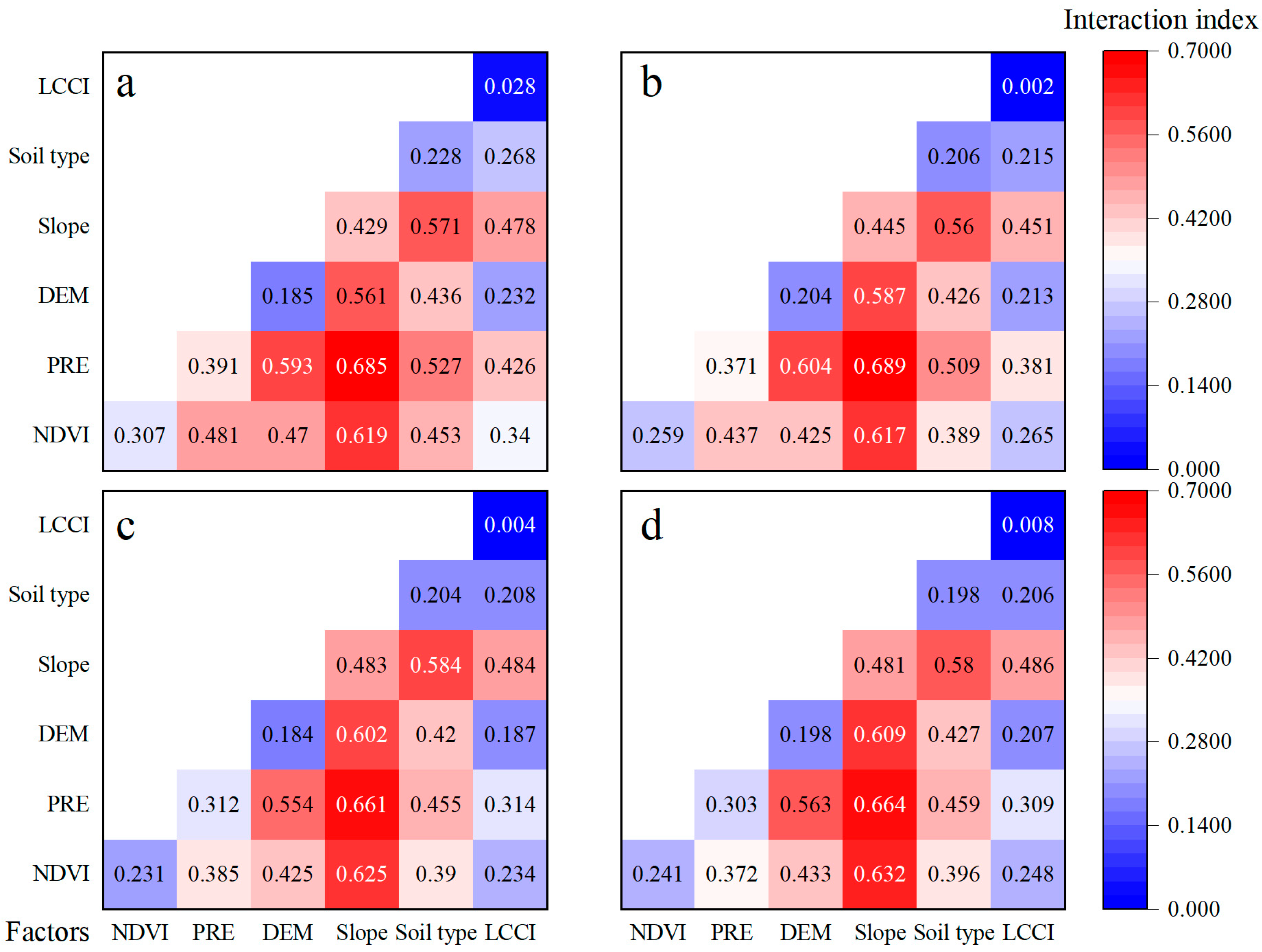
3.2.2. Interaction Analysis

The interaction of both factors revealed a better understanding of the spatial differentiation of SC compared to the single factor (Figure 8). In 2000–2020, the interaction index of slope with average annual precipitation reaches 0.685, which was obviously higher than the values of other interaction factors. Additionally, the interactions of slope with NDVI and DEM, soil type with slope and average annual precipitation, and DEM with average annual precipitation exhibited higher explanatory ability for the spatial variability of SC, with interaction indexes above 0.5. Furthermore, the interaction indexes of NDVI with average annual precipitation, DEM with soil type, average annual precipitation with LCCI, DEM with soil type, and slope with LCCI were at higher levels, surpassing 0.45. Conversely, the interaction indexes of LCCI with DEM and soil type were relatively weaker, measuring below 0.35.

Under the DDS, the interaction of average annual precipitation with slope, NDVI with slope, DEM with slope, average annual precipitation with DEM, and slope with soil type elucidated a greater spatial variability in SC in the SYR. The interaction of average annual precipitation with slope exhibited the higher values, measuring 0.689, 0.661, and 0.664 for the ECS, NCS, and EES, respectively. Besides, the interaction of LCCI with soil type and DEM exhibited the least explanatory ability for spatial variability of SC under the DDS, approximately 0.2.

3.3. Suitable Zones Analysis

The analysis demonstrated considerable variations in the amount of SC based on the adaption range or type of drivers (

Table 7. Adaption ranges/types of diverse influencing factors from 2000 to 2020 and under the DDS from 2021–2030.

Key Factors	2000–2020		ECS		NCS		EES
	Adaption range/Type	Annual Mean SC (t/(km2·a))	Adaption Range/Type	Annual Mean SC (t/(km2·a))	Adaption Range/Type	Annual Mean SC (t/(km2·a))	Adaption Range/Type	Annual Mean SC t/(km2·a))
NDVI	0.72–0.77	6156.48	0.91–1	4617.37	0.75–0.82	4176.26	0.72–0.87	4454.95
PRE (mm)	763.40–928.07	8849.23	822.30–1020.70	5624.14	946.08–1081	5397.29	766.42–866.17	5156.79
DEM (m)	3908–4111	7394.14	3908–4111	5391.86	3908–4111	5144.8	3908–4111	5504.33
Slope (°)	44.86–56.08	9835.02	44.86–56.08	7152.83	44.86–56.08	6927.98	44.86–56.08	7338.02
Soil type	Black felt soil	6513.22	Black felt soil	4646.98	Black felt soil	4131.56	Black felt soil	4409.63
LCCI (%)	0.052–0.16	5267.39	1.27–2.52	5450.69	0.12–0.39	5359.39	0.14–0.51	4548.03

). From 2000 to 2020, the mean SC reached its maximum values of 6156 t/(km²·a), 8849 t/(km²·a), and 9835 t/(km²·a) during the NDVI range of 0.72–0.77, the average annual precipitation range of 763.40–928.07 mm, and slope range of 44.86–56.08°, respectively. The influences of NDVI, average annual precipitation, and slope on SC under the DDS were similar to the 2000–2020 period, with the differences in the magnitude of the effects. In the ECS, higher average SC was observed with higher NDVI, while more abundant average annual precipitation in the ECS resulted in significantly greater SC compared to other scenarios. The EES showed greater average SC with steeper slope. The DEM interval of 3908–4111 m generated higher average SC values under the DDS, and black felt soil exhibited higher SC capacity. Additionally, the effect of LUCC on SC is characterized by LCCI > 0, indicating high SC capacity when ecological improvement occurs.

As shown in Figure 9, the SC suitability indexes for the DDS exhibited similar distributional characteristics. Areas with high SC suitability index were primarily assigned in the center and east parts of the SYR, with the southeastern region having the highest SC suitability index. The distribution of areas with higher SC suitability index was smaller, while the range of SC unsuitable areas was larger than the distribution of SC suitable areas. The region of the SC unsuitable (N-value) zones under the DDS was approximately 60,000 km², exceeding 50% of the area of the SYR.

4. Discussion

4.1. SpatioTemporal Variation in SC in the SYR

The spatial distribution of SC in the SYR presented a pattern of gradual decrease from the center towards the surrounding, which corresponded to the distribution of slope (Figure 10a). The finding demonstrates that areas with higher slopes tend to maintain stronger SC capacity and aligns with previous research results [20]. Slope emerged as the dominant factor driving the spatial variability of SC. As slope increases, the spatial differentiation of SC becomes more pronounced [60,61]. The intensity of soil erosion tends to escalate with steeper slope gradients [62], and the gravitational impact of higher slope predisposes them to soil erosion phenomena [63]. Additionally, slope influences the transformation of material and energy on the surface, leading to alteration in soil texture and influencing vegetation distribution [64]. The high slope zone (31.45°–56.06°) in the center of the SYR, located in the valley, is predominantly covered by woodland, scrub, and high coverage grassland (Figure 10b). This region benefits from the strong water retention and soil stabilization capacity of these vegetation types, while the valley area provides sufficient water for conducive growing conditions. Consequently, the high slope area of the SYR exhibits a strong SC capacity.

In contrast, the northwest of the SYR, characterized by high altitude and inland location, exhibits relatively weak SC capacity due to natural conditions of water scarcity and low vegetation cover. Research indicated that precipitation is an essential water source in semi-arid regions and cumulative infiltration of rainwater on the surface is critical for vegetation conservation, reduction of soil erosion, and sustainable regional development [65]. As a typical semi-arid region, the SYR experiences water scarcity in the northwest and relatively abundant water resources and precipitation in the southeast (Figure 10d). This results in a decrease in NDVI from southeast to northwest in the SYR (Figure 10c). The average annual SC in the northwest of the SYR (Madoi, Qumarleb, and Chindu counties) estimated in this study was 982 t/(km²·a), which is lower than the overall average. This aligns with previous research [66] that used RUSLE to estimate the average annual SC (920 t/(km²·a)) in the SYR national park (located in Madoi, Qumarleb, and Chindu counties) from 2000 to 2015 (

Table 8. Comparison of research results.

Research area	Method	Research Period	Average Annual Total SC/(t/a)	Average Annual Average SC/(t/(km2·a))	This Study
Yellow river national park (include Madoi, Qumarleb and Chindu) [67]	RUSLE	2000–2015	——	920	982 t/(km2·a)
Upper Yellow River region [38]	RUSLE	2000–2019	——	2281	2765 t/(km2·a)
QTP [20]	RUSLE	2000–2015	12.07 × 109	3908	28.47 × 108 t/a and 2765 t/(km2·a).

). It is important to note that differences in research methods and study scales can lead to variations in the estimation of SC services. In this study, the average annual SC in the SYR from 2000 to 2020 was estimated as 2765 t/(km²·a), slightly higher than the average annual SC (2281 t/(km²·a)) in the upstream region of Yellow River reported in the previous study [38] for 2000–2019. This difference can be attributed to the inclusion of the SYR and some parts of the Loess Plateau in the study area.

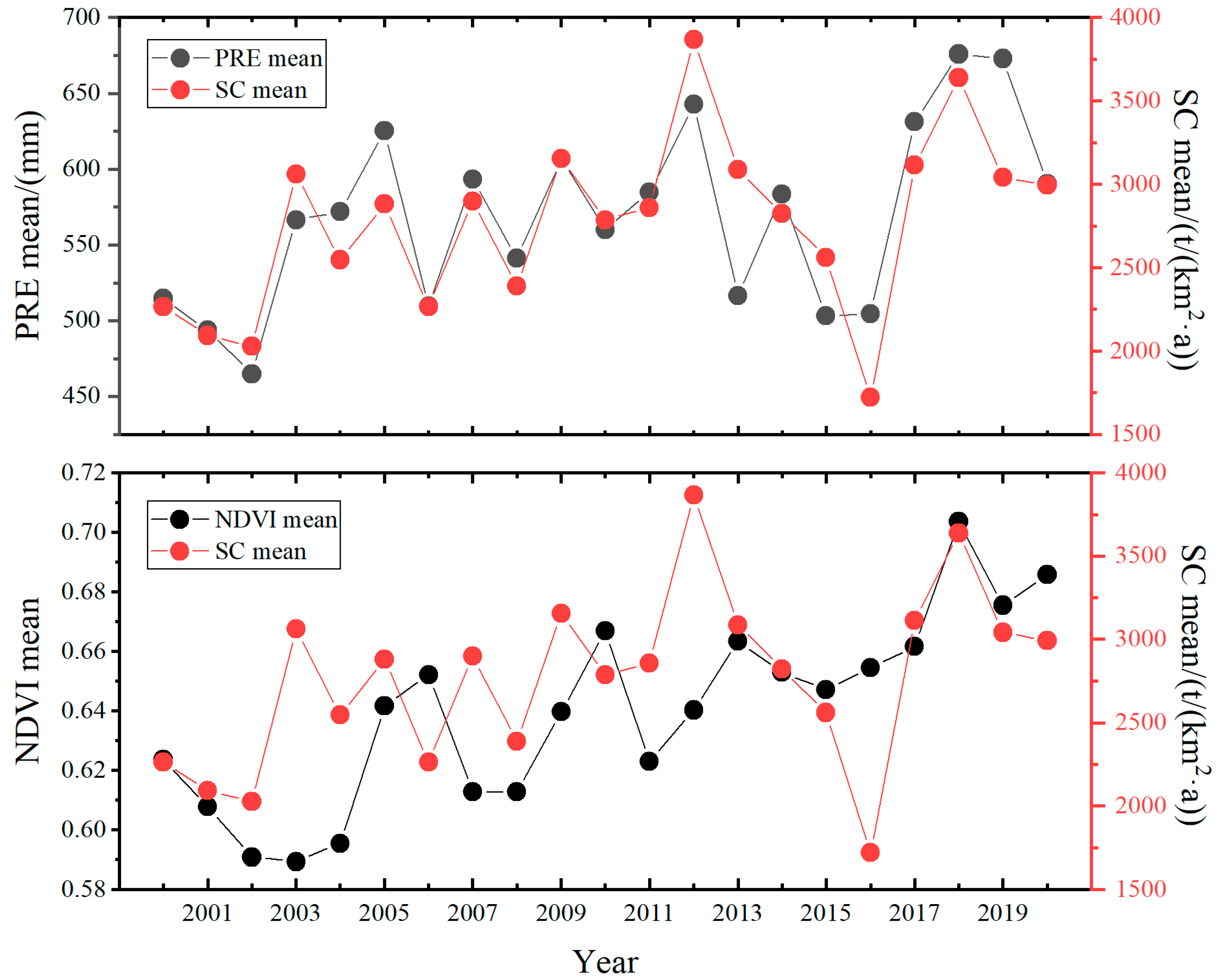
4.2. Impact of Precipitation and NDVI on SC

Due to the slow temporal changes in the topography, land use type, and soil texture of the SYR, the erosion factors resulting from these factors are considered to be temporally invariant. Consequently, the most influential factors affecting SC are identified as precipitation and NDVI. Given the sparse vegetation cover in many regions of the SYR, precipitation emerges as the primary determinant of SC in these areas. For instance, the northwestern part of the SYR where NDVI values can be below 0.2 (Figure 10c). Although there exist slight fluctuations (+10% and −10%) under extreme climate scenarios (ECS and EES), their extent remains limited. NDVI values at lower levels essentially have negligible effects on SC. Consequently, precipitation becomes the dominant factor influencing SC in these low NDVI regions. Figure 11 demonstrated a significant disparity in precipitation between the ECS and NCS scenarios. Greater precipitation has a decreasing impact on SC in low NDVI regions, leading to the observation that the SC under the ECS scenario, characterized by relatively high NDVI levels, is lower than that under the NCS scenario due to the influence of increased precipitation.

The annual precipitation and NDVI are key factors influencing SC [14]. They exhibit similar trends, with NDVI following the same trend annually as precipitation increases or decreases, and SC also reflecting these changes (Figure 12). Previous research demonstrated that SC function of ecosystem is closely related to vegetation condition, and suitable precipitation enhances the growth of alpine vegetation [21]. The promotion of alpine vegetation coverage expands the area covered by surface vegetation, effectively reducing the scouring effect of precipitation on topsoil, thus maintaining regional SC capacity [68]. In regions with high vegetation cover, dense vegetation canopies and plant dieback significantly reduce the kinetic energy of precipitation, prolonging the time for precipitation to infiltrate the soil, thereby providing a strong rainwater retaining capacity [69]. High vegetation cover can mitigate soil erosion, and reduced soil erosion can promote vegetation growth, creating a positive feedback loop that stabilizes ecosystem development [70]. The spatial distribution pattern and change trend of NDVI in the SYR from 2000 to 2020 align with the SC, indicating that enhancing vegetation coverage to a certain extent contributes to regional SC enhancement.

4.3. Multiple Factors Influence on SC

Geographical processes are influenced by a multitude of factors [71]. A previous study revealed that the derivation and transformation of ecosystem services result from a combined effects of diverse components [72]. From a comparison of the effects of single factors and double factors (Table 6 and Figure 8), it is evident that the interaction between double factors has a stronger explanatory ability of SC than individual factors alone. Interaction analyses demonstrated that the interaction between precipitation with slope, which dominates the spatiotemporal variability of SC in the SYR, is significantly more influential than other factors. Related research indicated a positive correlation between surface runoff and slope [15]. Surface runoff occurs when precipitation flows over the ground, and areas with steeper slopes experience faster runoff rates, leading to a higher probability of soil loss. Moreover, this study found that the interaction between NDVI and slope contributes to explaining SC services. Vegetation cover plays a crucial role in mitigating soil loss and surface runoff [14]. Vegetation reduces the erosive impact of rainfall on the surface and facilitates the infiltration of rainwater into the soil, thereby reducing soil loss, particularly in areas with steep slopes [73]. Additionally, the interaction between slope and DEM, and DEM and average annual precipitation, exhibits a greater explanatory ability for spatial variability in SC. On one hand, areas with greater topographic relief tend to maintain greater and longer slopes, resulting in higher kinetic energy of surface runoff and greater sediment accumulation [74]. On the other hand, the high slope area in the center of the SYR, situated at an altitude of approximately 4000 m, receives abundant precipitation and water, and the favorable water and heat conditions promote vegetation growth [75]. Consequently, these areas are characterized by high suitability for SC and possess high SC value.

4.4. Recommendations for Future SC Measures

Comparing the results of SC estimation under the DDS (Figure 6), it is observed that the regions with a decreased trend in SC in the future are predominantly located in the grassland and bare land areas in the southeast and south of the SYR. Interestingly, these areas are classified as high SC suitability zones, as revealed by the results presented in Figure 9. This phenomenon, which leads to a decline in SC function in areas with high SC suitability, is likely attributed to excessive precipitation and high soil moisture levels. The southeast of the SYR belongs to the plateau sub-frigid zone with a humid monsoon climate and the largest peat mire in China. Consequently, heavy precipitation leads to regional water accumulation, while prolonged high soil moisture content contributes to reduced vegetation cover [76], ultimately resulting in soil erosion. The National Park in China is situated in the northwest of the SYR, characterized by low SC and belonging to the non-suitable (N) zone of SC. This region, located at an altitude exceeding 4000 m, lies in the continental hinterland and is less affected by the moisture brought by the warm currents from the Indian and Pacific Oceans, resulting in a relatively arid climate [77]. Under the NCS, SC services in the northwest of the SYR demonstrate both increasing and decreasing trends, depending on the specific scenario. This can be predominantly attributed to the strong influence of topographical and climatic factors on SC. The SC capacity is restricted by low temperatures, limited water, and poor vegetation. Alpine regions experience limited vegetation growth due to low temperatures [78], while water deficits lead to reduced soil moisture content [71]. Concomitantly, reduced moisture availability negatively impacts vegetation survival [79], thereby increasing the frequency of soil erosion. Conversely, suitable precipitation promotes the growth of alpine vegetation [76], which, in turn, enhances the stabilizing effect of vegetation on the soil. Furthermore, the RUSLE model exhibits a strongly correlation with precipitation, soil, topography, and vegetation data, with the rainfall erosion factor showing the strongest linear relationship. However, precipitation data contains variability depending on computation methods and spatial resolution, which contributes to the uncertainty in the SC estimation results. The implementation of precipitation monitoring in the SYR provides some indication of regional SC measures.

5. Conclusions

This study evaluated the spatiotemporal characteristics of SC services in the SYR by employing the RUSLE model, and the spatiotemporal evolutionary trends of SC service and their driving factors were evaluated using trend analysis and geographical detector, respectively. The research findings indicated that:

During 2000–2020, the spatial heterogeneity of SC services in the SYR was characterized by the distribution of “gradually decreasing from Southeast to Northwest”, and demonstrated a trend of “increasing, decreasing, and then increasing”, with more than 90% of the area demonstrating an increasing trend. Under the DDS for 2021–2030, the variation trend of SC services in the SYR is predominantly increasing, and its growth trend is, from highest to lowest: NCS > ECS > EES.

Slope was the most significant factor contributing to spatial heterogeneity in SC services, followed by average annual precipitation and NDVI, with the LCCI having the least influence. Under the DDS, the single factor drivers of slope and average annual precipitation are in a fluctuating state, but still alternately dominate the spatial variability of SC services in the SYR. Overall, the interaction between double variables was stronger than the single factor explanatory ability, and the interaction of slope with average annual precipitation and NDVI on the spatiotemporal heterogeneity of SC in the SYR had the strongest explanatory ability.

The average value of SC services in the SYR reached the maximum when the NDVI, average annual precipitation, DEM, and slope were 0.72–0.77, 763.40–928.07 mm, 3908–4111 m, and 44.86–56.08°, respectively, including when the soil type was black felted soil and the LCCI was 0.052–0.16%.

Through scenario simulation, this study achieved improved simulation results, providing insights into the driving factors behind SC changes and their spatiotemporal variations under different development scenarios in the SYR, both historically and in the future. The findings hold significant guidance for ecological and environmental management, and sustainable development, in the SYR. Furthermore, the scenarios and methodologies employed in this research serve as valuable references for investigations in other study areas and related disciplines.

References

1. Costanza, R.; d’Arge, R.; De Groot, R.; Farber, S.; Grasso, M.; Hannon, B.; Limburg, K.; Naeem, S.; O’neill, R.V.; Paruelo, J. The value of the world’s ecosystem services and natural capital. Nature 1997, 387, 253–260. [Google Scholar] [CrossRef]
2. Ganasri, B.P.; Ramesh, H. Assessment of soil erosion by RUSLE model using remote sensing and GIS—A case study of Nethravathi Basin. Geosci. Front. 2016, 7, 953–961. [Google Scholar] [CrossRef]
3. Yin, C.; Zhao, W.; Pereira, P. Soil conservation service underpins sustainable development goals. Glob. Ecol. Conserv. 2022, 33, e01974. [Google Scholar] [CrossRef]
4. Yang, L.; Wang, D.; Wang, Z. Quantitative assessment of the supply-demand relationship of soil conservation service in the Sushui River Basin. Resour. Sci. 2020, 42, 2451–2462. [Google Scholar] [CrossRef]
5. Chen, J.; Yang, Y.; Feng, Z.; Huang, R.; Zhou, G.; You, H.; Han, X. Ecological Risk Assessment and Prediction Based on Scale Optimization—A Case Study of Nanning, a Landscape Garden City in China. Remote Sens. 2023, 15, 1304. [Google Scholar] [CrossRef]
6. Pimentel, D. Soil Erosion: A Food and Environmental Threat. Environ. Dev. Sustain. 2006, 8, 119–137. [Google Scholar] [CrossRef]
7. Yang, Y.; Chen, J.; Lan, Y.; Zhou, G.; You, H.; Han, X.; Wang, Y.; Shi, X. Landscape Pattern and Ecological Risk Assessment in Guangxi Based on Land Use Change. Int. J. Environ. Res. Public Health 2022, 19, 1595. [Google Scholar] [CrossRef] [PubMed]
8. An, Y.; Zhao, W.; Li, C.; Ferreira, C.S.S. Temporal changes on soil conservation services in large basins across the world. Catena 2022, 209, 105793. [Google Scholar] [CrossRef]
9. Yang, D.; Kanae, S.; Oki, T.; Koike, T.; Musiake, K. Global potential soil erosion with reference to land use and climate changes. Hydrol. Process. 2003, 17, 2913–2928. [Google Scholar] [CrossRef]
10. Wang, H.; Gao, J.; Hou, W. Quantitative attribution analysis of soil erosion in different geomorphological types in karst areas: Based on the geodetector method. J. Geogr. Sci. 2019, 29, 271–286. [Google Scholar] [CrossRef]
11. Bai, Z.; Dent, D. Recent land degradation and improvement in China. Ambio 2009, 38, 150–156. [Google Scholar] [CrossRef] [PubMed]
12. Yi, X.S.; Li, G.S.; Yin, Y.Y. The impacts of grassland vegetation degradation on soil hydrological and ecological effects in the source region of the Yellow River—A case study in Junmuchang region of Maqin country. Procedia Environ. Sci. 2012, 13, 967–981. [Google Scholar] [CrossRef]
13. McGuire, A.D.; Sturm, M.; Chapin, F.S., III. Arctic Transitions in the Land–Atmosphere System (ATLAS): Background, objectives, results, and future directions. J. Geophys. Res. Atmos. 2003, 108, D2. [Google Scholar] [CrossRef]
14. Chen, H.; Zhang, X.; Abla, M.; Lü, D.; Yan, R.; Ren, Q.; Ren, Z.; Yang, Y.; Zhao, W.; Lin, P.; et al. Effects of vegetation and rainfall types on surface runoff and soil erosion on steep slopes on the Loess Plateau, China. Catena 2018, 170, 141–149. [Google Scholar] [CrossRef]
15. El Kateb, H.; Zhang, H.; Zhang, P.; Mosandl, R. Soil erosion and surface runoff on different vegetation covers and slope gradients: A field experiment in Southern Shaanxi Province, China. Catena 2013, 105, 1–10. [Google Scholar] [CrossRef]
16. Shi, P.; Zhang, Y.; Ren, Z.; Yu, Y.; Li, P.; Gong, J. Land-use changes and check dams reducing runoff and sediment yield on the Loess Plateau of China. Sci. Total Environ. 2019, 664, 984–994. [Google Scholar] [CrossRef]
17. Sun, P.; Wu, Y.; Gao, J.; Yao, Y.; Zhao, F.; Lei, X.; Qiu, L. Shifts of sediment transport regime caused by ecological restoration in the Middle Yellow River Basin. Sci. Total Environ. 2020, 698, 134261. [Google Scholar] [CrossRef]
18. Kang, H.; Pan, T.; Gai, A.; Liu, Y. Effects of ecological degradation and restoration on soil conservation function in Three Rivers Head-water region. Bull. Soil Water Conserv. 2017, 37, 7–14. [Google Scholar]
19. Huang, C.; Zhao, D.; Liao, Q.; Xiao, M. Linking landscape dynamics to the relationship between water purification and soil retention. Ecosyst. Serv. 2023, 59, 101498. [Google Scholar] [CrossRef]
20. Lu, R.; Dai, E.; Wu, C. Spatial and temporal evolution characteristics and driving factors of soil conservation services on the Qinghai-Tibet Plateau. Catena 2023, 221, 106766. [Google Scholar] [CrossRef]
21. Durigon, V.; Carvalho, D.; Antunes, M.; Oliveira, P.; Fernandes, M. NDVI time series for monitoring RUSLE cover management factor in a tropical watershed. Int. J. Remote Sens. 2014, 35, 441–453. [Google Scholar] [CrossRef]
22. Aksoy, H.; Kavvas, M.L. A review of hillslope and watershed scale erosion and sediment transport models. Catena 2005, 64, 247–271. [Google Scholar] [CrossRef]
23. Sujatha, E.R.; Sridhar, V. Spatial Prediction of Erosion Risk of a Small Mountainous Watershed Using RUSLE: A Case-Study of the Palar Sub-Watershed in Kodaikanal, South India. Water 2018, 10, 1608. [Google Scholar] [CrossRef]
24. Evans, R.; Collins, A.L.; Zhang, Y.; Foster, I.D.L.; Boardman, J.; Sint, H.; Lee, M.R.F.; Griffith, B.A. A comparison of conventional and 137Cs-based estimates of soil erosion rates on arable and grassland across lowland England and Wales. Earth-Sci. Rev. 2017, 173, 49–64. [Google Scholar] [CrossRef]
25. Peng, T.; Wang, S.-J. Effects of land use, land cover and rainfall regimes on the surface runoff and soil loss on karst slopes in southwest China. Catena 2012, 90, 53–62. [Google Scholar] [CrossRef]
26. Merritt, W.S.; Letcher, R.A.; Jakeman, A.J. A review of erosion and sediment transport models. Environ. Model. Softw. 2003, 18, 761–799. [Google Scholar] [CrossRef]
27. Zeng, C.; Wang, S.; Bai, X.; Li, Y.; Tian, Y.; Li, Y.; Wu, L.; Luo, G. Soil erosion evolution and spatial correlation analysis in a typical karst geomorphology using RUSLE with GIS. Solid Earth 2017, 8, 721–736. [Google Scholar] [CrossRef]
28. Atoma, H.; Suryabhagavan, K.; Balakrishnan, M. Soil erosion assessment using RUSLE model and GIS in Huluka watershed, Central Ethiopia. Sustain. Water Resour. Manag. 2020, 6, 12. [Google Scholar] [CrossRef]
29. Abu Hammad, A. Watershed erosion risk assessment and management utilizing revised universal soil loss equation-geographic information systems in the Mediterranean environments. Water Environ. J. 2011, 25, 149–162. [Google Scholar] [CrossRef]
30. Luvai, A.; Obiero, J.; Omuto, C. Soil Loss Assessment Using the Revised Universal Soil Loss Equation (RUSLE) Model. Appl. Environ. Soil Sci. 2022, 2022, 2122554. [Google Scholar] [CrossRef]
31. Liu, B.; Xie, Y.; Li, Z.; Liang, Y.; Zhang, W.; Fu, S.; Yin, S.; Wei, X.; Zhang, K.; Wang, Z.; et al. The assessment of soil loss by water erosion in China. Int. Soil Water Conserv. Res. 2020, 8, 430–439. [Google Scholar] [CrossRef]
32. Ma, X.; Zhao, C.; Zhu, J. Aggravated risk of soil erosion with global warming—A global meta-analysis. Catena 2021, 200, 105129. [Google Scholar] [CrossRef]
33. Wang, Y.; Wang, X.; Yin, L.; Feng, X.; Zhou, C.; Han, L.; Lü, Y. Determination of conservation priority areas in Qinghai Tibet Plateau based on ecosystem services. Environ. Sci. Policy 2021, 124, 553–566. [Google Scholar] [CrossRef]
34. Fu, B.J.; Zhao, W.W.; Chen, L.D.; Zhang, Q.J.; Lü, Y.H.; Gulinck, H.; Poesen, J. Assessment of soil erosion at large watershed scale using RUSLE and GIS: A case study in the Loess Plateau of China. Land Degrad. Dev. 2005, 16, 73–85. [Google Scholar] [CrossRef]
35. Hu, S.; Li, L.; Chen, L.; Cheng, L.; Yuan, L.; Huang, X.; Zhang, T. Estimation of Soil Erosion in the Chaohu Lake Basin through Modified Soil Erodibility Combined with Gravel Content in the RUSLE Model. Water 2019, 11, 1806. [Google Scholar] [CrossRef]
36. Shi, Z.H.; Cai, C.F.; Ding, S.W.; Wang, T.W.; Chow, T.L. Soil conservation planning at the small watershed level using RUSLE with GIS: A case study in the Three Gorge Area of China. Catena 2004, 55, 33–48. [Google Scholar] [CrossRef]
37. Guo, Y.; Peng, C.; Zhu, Q.; Wang, M.; Wang, H.; Peng, S.; He, H. Modelling the impacts of climate and land use changes on soil water erosion: Model applications, limitations and future challenges. J. Environ. Manag. 2019, 250, 109403. [Google Scholar] [CrossRef] [PubMed]
38. Liu, S.; Shao, Q.; Ning, J.; Niu, L.; Zhang, X.; Liu, G.; Huang, H. Remote-Sensing-Based Assessment of the Ecological Restoration Degree and Restoration Potential of Ecosystems in the Upper Yellow River over the Past 20 Years. Remote Sens. 2022, 14, 3550. [Google Scholar] [CrossRef]
39. Hao, R.; Yu, D.; Liu, Y.; Liu, Y.; Qiao, J.; Wang, X.; Du, J. Impacts of changes in climate and landscape pattern on ecosystem services. Sci. Total Environ. 2017, 579, 718–728. [Google Scholar] [CrossRef] [PubMed]
40. Lyu, R.; Clarke, K.C.; Zhang, J.; Feng, J.; Jia, X.; Li, J. Spatial correlations among ecosystem services and their socio-ecological driving factors: A case study in the city belt along the Yellow River in Ningxia, China. Appl. Geogr. 2019, 108, 64–73. [Google Scholar] [CrossRef]
41. Wang, J.; Xu, C. Geodetector: Principle and prospective. Acta Geogr. Sin. 2017, 72, 116–134. [Google Scholar]
42. Fotheringham, A.S.; Charlton, M.E.; Brunsdon, C. Geographically Weighted Regression: A Natural Evolution of the Expansion Method for Spatial Data Analysis. Environ. Plan A Econ. Space 1998, 30, 1905–1927. [Google Scholar] [CrossRef]
43. Liu, W.; Zhan, J.; Zhao, F.; Wang, C.; Zhang, F.; Teng, Y.; Chu, X.; Kumi, M.A. Spatio-temporal variations of ecosystem services and their drivers in the Pearl River Delta, China. J. Clean. Prod. 2022, 337, 130466. [Google Scholar] [CrossRef]
44. Zhao, Y.; Liu, L.; Kang, S.; Ao, Y.; Han, L.; Ma, C. Quantitative Analysis of Factors Influencing Spatial Distribution of Soil Erosion Based on Geo-Detector Model under Diverse Geomorphological Types. Land 2021, 10, 604. [Google Scholar] [CrossRef]
45. Gao, J.; Jiang, Y.; Anker, Y. Contribution analysis on spatial tradeoff/synergy of Karst soil conservation and water retention for various geomorphological types: Geographical detector application. Ecol. Indic. 2021, 125, 107470. [Google Scholar] [CrossRef]
46. Chu, H.; Wei, J.; Li, T.; Jia, K. Application of Support Vector Regression for Mid- and Long-term Runoff Forecasting in “Yellow River Headwater” Region. Procedia Eng. 2016, 154, 1251–1257. [Google Scholar] [CrossRef]
47. Luo, D.; Jin, H.; Bense, V.F.; Jin, X.; Li, X. Hydrothermal processes of near-surface warm permafrost in response to strong precipitation events in the Headwater Area of the Yellow River, Tibetan Plateau. Geoderma 2020, 376, 114531. [Google Scholar] [CrossRef]
48. Qin, Q.; Chen, J.; Yang, Y.; Zhao, X.; Zhou, G.; You, H.; Han, X. Spatiotemporal variations of vegetation and its response to topography and climate in the source region of the Yellow River. China Environ. Sci. 2021, 41, 3832–3841. [Google Scholar]
49. Hou, J.; Chen, J.; Zhang, K.; Zhou, G.; You, H.; Han, X. Temporal and Spatial Variation Characteristics of Carbon Storage in the Source Region of the Yellow River Based on InVEST and GeoSoS-FLUS Models and Its Response to Different Future Scenarios. Huan Jing Ke Xue Huanjing Kexue 2022, 43, 5253–5262. [Google Scholar]
50. Lin, X.; Chen, J.; Lou, P.; Yi, S.; Qin, Y.; You, H.; Han, X. Improving the estimation of alpine grassland fractional vegetation cover using optimized algorithms and multi-dimensional features. Plant Methods 2021, 17, 96. [Google Scholar] [CrossRef]
51. Liu, J.; Zhang, Z.; Xu, X.; Kuang, W.; Zhou, W.; Zhang, S.; Li, R.; Yan, C.; Yu, D.; Wu, S. Spatial patterns and driving forces of land use change in China during the early 21st century. J. Geogr. Sci. 2010, 20, 483–494. [Google Scholar] [CrossRef]
52. Shao, Q.; Zhiping, Z.; Jiyuan, L.; Jiangwen, F. The characteristics of land cover and macroscopical ecology changes in the source region of three rivers on Qinghai-Tibet Plateau during last 30 years. Geogr. Res. 2010, 29, 1439–1451. [Google Scholar]
53. Renard, K.G.; Laflen, J.; Foster, G.; McCool, D. The revised universal soil loss equation. In Soil Erosion Research Methods; Routledge: London, UK, 2017; pp. 105–126. [Google Scholar]
54. Wischmeier, W.H.; Johnson, C.; Cross, B. Soil Erodibility Nomograph for Farmland and Construction Sites; National Academies of Sciences, Engineering, and Medicine: Washington, DC, USA, 1971. [Google Scholar]
55. Williams, J.R.; Greenwood, D.J.; Nye, P.H.; Walker, A. The erosion-productivity impact calculator (EPIC) model: A case history. Philos. Trans. R. Soc. Lond. B Biol. Sci. 1990, 329, 421–428. [Google Scholar]
56. Van Remortel, R.D.; Hamilton, M.E.; Hickey, R.J. Estimating the LS factor for RUSLE through iterative slope length processing of digital elevation data within Arclnfo grid. Cartography 2001, 30, 27–35. [Google Scholar] [CrossRef]
57. Van der Knijff, J.; Jones, R.; Montanarella, L. Soil erosion risk: Assessment in Europe. In European Soil Bureau; European Commission: Brussels, Belgium, 2000. [Google Scholar]
58. Theil, H. A rank-invariant method of linear and polynomial regression analysis. In Henri Theil’s Contributions to Economics and Econometrics; Springer: Berlin/Heidelberg, Germany, 1992; pp. 345–381. [Google Scholar]
59. Sen, P.K. Estimates of the regression coefficient based on Kendall’s tau. J. Am. Stat. Assoc. 1968, 63, 1379–1389. [Google Scholar] [CrossRef]
60. Wu, L.; He, Y.; Ma, X. Can soil conservation practices reshape the relationship between sediment yield and slope gradient? Ecol. Eng. 2020, 142, 105630. [Google Scholar] [CrossRef]
61. Chen, Z.; Zhu, B.; Tang, J.; Liu, X. Influence of slope gradient on soil erosion in the hilly area of purple soil under natural rainfall. Pearl River 2016, 37, 29–33. [Google Scholar]
62. Fox, D.M.; Bryan, R.B. The relationship of soil loss by interrill erosion to slope gradient. Catena 2000, 38, 211–222. [Google Scholar] [CrossRef]
63. Wu, L.; Peng, M.; Qiao, S.; Ma, X.-Y. Effects of rainfall intensity and slope gradient on runoff and sediment yield characteristics of bare loess soil. Environ. Sci. Pollut. Res. 2018, 25, 3480–3487. [Google Scholar] [CrossRef] [PubMed]
64. Ostendorf, B.; Reynolds, J.F. A model of arctic tundra vegetation derived from topographic gradients. Landsc. Ecol. 1998, 13, 187–201. [Google Scholar] [CrossRef]
65. Kalhoro, S.A.; Ding, K.; Zhang, B.; Chen, W.; Hua, R.; Shar, A.H.; Xu, X. Soil infiltration rate of forestland and grassland over different vegetation restoration periods at Loess Plateau in northern hilly areas of China. Landsc. Ecol. Eng. 2019, 15, 91–99. [Google Scholar] [CrossRef]
66. Cao, J.; Adamowski, J.F.; Deo, R.C.; Xu, X.; Gong, Y.; Feng, Q. Grassland Degradation on the Qinghai-Tibetan Plateau: Reevaluation of Causative Factors. Rangel. Ecol. Manag. 2019, 72, 988–995. [Google Scholar] [CrossRef]
67. Cao, W.; Liu, L.; Wu, D.; Huang, L. Spatial and temporal variations and the importance of hierarchy of ecosystem functions in the Three-river-source National Park. Acta Ecol. Sin 2019, 39, 1361–1374. [Google Scholar]
68. Li, C.; Wu, Y.; Gao, B.; Zheng, K.; Wu, Y.; Li, C. Multi-scenario simulation of ecosystem service value for optimization of land use in the Sichuan-Yunnan ecological barrier, China. Ecol. Indic. 2021, 132, 108328. [Google Scholar] [CrossRef]
69. Hartanto, H.; Prabhu, R.; Widayat, A.S.E.; Asdak, C. Factors affecting runoff and soil erosion: Plot-level soil loss monitoring for assessing sustainability of forest management. For. Ecol. Manag. 2003, 180, 361–374. [Google Scholar] [CrossRef]
70. Zhu, Q.; Zhou, Z.; Liu, T.; Bai, J. Vegetation restoration and ecosystem soil conservation service value increment in Yanhe Watershed, Loess Plateau. Acta Ecol. Sin 2021, 41, 2557–2570. [Google Scholar]
71. Dai, E.; Wang, Y. Spatial heterogeneity and driving mechanisms of water yield service in the Hengduan Mountain region. Acta Geogr. Sin 2020, 75, 607–619. [Google Scholar]
72. Fu, B.; Liu, Y.; Lü, Y.; He, C.; Zeng, Y.; Wu, B. Assessing the soil erosion control service of ecosystems change in the Loess Plateau of China. Ecol. Complex. 2011, 8, 284–293. [Google Scholar] [CrossRef]
73. Mohammad, A.G.; Adam, M.A. The impact of vegetative cover type on runoff and soil erosion under different land uses. Catena 2010, 81, 97–103. [Google Scholar] [CrossRef]
74. Ma, X.; Li, Y.; Li, B.; Han, W.; Liu, D.; Gan, X. Nitrogen and phosphorus losses by runoff erosion: Field data monitored under natural rainfall in Three Gorges Reservoir Area, China. Catena 2016, 147, 797–808. [Google Scholar] [CrossRef]
75. Zuo, Y.; Li, Y.; He, K.; Wen, Y. Temporal and spatial variation characteristics of vegetation coverage and quantitative analysis of its potential driving forces in the Qilian Mountains, China, 2000–2020. Ecol. Indic. 2022, 143, 109429. [Google Scholar] [CrossRef]
76. Liu, Y.; Liu, S.; Sun, Y.; Li, M.; An, Y.; Shi, F. Spatial differentiation of the NPP and NDVI and its influencing factors vary with grassland type on the Qinghai-Tibet Plateau. Environ. Monit. Assess. 2021, 193, 48. [Google Scholar] [CrossRef] [PubMed]
77. An, R.; Wang, H.-L.; Feng, X.-Z.; Wu, H.; Wang, Z.; Wang, Y.; Shen, X.-J.; Lu, C.-H.; Quaye-Ballard, J.A.; Chen, Y.-H. Monitoring rangeland degradation using a novel local NPP scaling based scheme over the “Three-River Headwaters” region, hinterland of the Qinghai-Tibetan Plateau. Quat. Int. 2017, 444, 97–114. [Google Scholar] [CrossRef]
78. Wang, D.; Li, X.; Zou, D.; Wu, T.; Xu, H.; Hu, G.; Li, R.; Ding, Y.; Zhao, L.; Li, W.; et al. Modeling soil organic carbon spatial distribution for a complex terrain based on geographically weighted regression in the eastern Qinghai-Tibetan Plateau. Catena 2020, 187, 104399. [Google Scholar] [CrossRef]
79. Pan, T.; Hou, S.; Wu, S.; Liu, Y.; Liu, Y.; Zou, X.; Herzberger, A.; Liu, J. Variation of soil hydraulic properties with alpine grassland degradation in the eastern Tibetan Plateau. Hydrol. Earth Syst. Sci. 2017, 21, 2249–2261. [Google Scholar] [CrossRef]
Figure 1. Geography and distribution of administrative regions of the SYR.
Sustainability 16 00777 g001
Figure 2. Research framework. (Note: SSPs: diverse scenario, LUCC: land use/land cover, NCS: Natural change scenario, ECS: Ecological conservation scenario, EES: Economic expansion scenario, R: precipitation erosion factor, K: soil erodibility factor, LS: topographic factor, C: vegetation cover and management factor, P: soil and water conservation measures factor, LCCI: land cover change index, SC: soil conservation, RUSLE: revised universal soil loss equation, GD: Geographical detector.)
Sustainability 16 00777 g002
Figure 3. Spatial distribution of SC in the SYR.
Sustainability 16 00777 g003
Figure 4. Variation and trend of total annual SC in the SYR from 2000–2020.
Sustainability 16 00777 g004
Figure 5. Spatial variation trend of SC services on the SYR.
Sustainability 16 00777 g005
Figure 6. Spatiotemporal variation trend of SC services on the SYR under the DDS during 2021–2030 (The small bar chart shows that the total annual SC, and the regression line represents the variation trend of SC in the SYR in each scenario). (Note: ECS: Ecological conservation scenario, NCS: Natural change scenario, EES: Economic expansion scenario.).
Sustainability 16 00777 g006
Figure 7. Variations in the explanatory ability of SC (q) by single drivers from 2021 to 2030.
Sustainability 16 00777 g007
Figure 8. The interactive influencing factor explanatory power and ecological detection of SC in the SYR. (Note: (a): 2000–2020, (b): ECS 2021–2030, (c): NCS 2021–2030, (d): EES 2021–2030.)
Sustainability 16 00777 g008
Figure 9. Spatial distribution of SC suitability index in the SYR under the DDS, and histogram of SC suitable area statistics. (Note: N, the six influencing factors of the area demonstrated to be unsuitable. 1–6 represents that 1–6 kinds of influencing factors of the area demonstrated to be suitable.)
Sustainability 16 00777 g009
Figure 10. Spatial distribution of slope, LUC (2020), average NDVI (2000–2020) and precipitation (2000–2020) in the SYR.
Sustainability 16 00777 g010
Figure 11. Variations in annual precipitation and average annual precipitation under the DDS.
Sustainability 16 00777 g011
Figure 12. Temporal variation in annual average precipitation, NDVI, and SC on the SYR from 2000 to 2020.
Sustainability 16 00777 g012