Sales in Commercial Alleys and Their Association with Air Pollution: Case Study in South Korea

Abstract

We investigate the dynamic interplay between air pollution (PM₁₀) and income and their joint association with quarterly sales in commercial alleys, focusing on the pre-COVID-19 (2018–2019) and COVID-19 (2020–2021) periods in Seoul, South Korea. The objective of this study is to identify how air pollution and income collectively influence consumer spending patterns by looking at the increase and decrease in sales in commercial alleys, with a focus on contrasting these effects before and during the COVID-19 pandemic, utilizing advanced machine learning techniques for deeper insights. Using machine learning techniques, including random forest, extreme gradient boosting, catboost, and lightGBM, and employing explainable artificial intelligence (XAI), this study identifies shifts in the significance of predictor variables, particularly PM₁₀, before and during the pandemic. The results show that before the pandemic, PM₁₀ played a notable role in shaping sales predictions, highlighting the sensitivity of sales to air quality. However, during the pandemic, the importance of PM₁₀ decreased significantly, highlighting the transformative indirect impact of external events on consumer behavior. This study also examines the joint association of PM₁₀ and income with sales, revealing distinctive patterns in consumer responses to air quality changes during the pandemic. These findings highlight the need for dynamic modeling to capture evolving consumer behavior and provide valuable insights for businesses and policymakers navigating changing economic and environmental conditions. While this study’s focus is on a specific region and time frame, the findings emphasize the importance of adaptability in predictive models and contribute to understanding the complex interplay between environmental and economic factors in shaping consumer spending behavior.

1. Introduction

The interplay between socioeconomic factors and environmental conditions has a significant impact on people’s spending behaviors. Much attention has been paid to people’s expenditure behaviors. As commercial activities in the cities promote urban sustainability and the vitality of public space [1], an improved understanding of people’s expenditure behaviors can provide new ways of describing the economic shapes of cities [2] and support better planning of shopping facilities or location decisions [3]. Expenditure behaviors are influenced by socioeconomic (e.g., income, gender) factors [4] and different environmental conditions (e.g., weather conditions, air pollution) [5]. Importantly, these relationships often vary due to disruptive events (e.g., COVID-19), outbreaks [6], and natural disasters [7]. Among socioeconomic factors, income stands out as a particularly influential element, shaping how individuals and households adjust their spending in response to changing conditions, including during unprecedented global events such as the COVID-19 pandemic.

Income has been advocated as a significant factor for determining expenditure behaviors. There is no doubt that people with higher incomes spend more money than those with lower incomes [8]. Interestingly, the associations between income and expenditure behaviors changed during the COVID-19 pandemic. It was shown that high-income households tended to reduce their spending more than low-income households [9]. Not only that, but during the COVID-19 pandemic, stay-at-home orders in the United States may also have led to substantial changes in people’s expenditure on travel, grocery shopping, and other categories [10]. While income levels and pandemic-related changes were crucial in shaping expenditure patterns, it is equally important to consider environmental influences, particularly air pollution, which significantly alters consumer behaviors and preferences.

Moreover, environmental factors such as air pollution have a significant effect on human behaviors and consumption patterns [11,12,13]. People tend to adjust their behaviors to prevent air pollution exposure [11] and change their time allocation and expenditure [14,15]. Additionally, air pollution has been linked to an increase in medical expenditure [16] and health insurance and reduced outdoor activities [17,18,19,20]. Air pollution has been found to have indirect effects on consumer behavior. Studies have shown that air pollution can disrupt consumption behaviors, leading to statistically significant economic effects [21]. Air pollution has a wide-ranging impact on consumer decision-making behavior, including health risks, emotional changes, changes in daily habits, and individual and group consumption behaviors [13]. Research has shown that air pollution increases customer feelings of anxiety and discomfort, leading to an increase in online shopping activity when consumers choose to decrease or avoid outdoor consumption [22]. Online public attention to air pollution plays a mediating role in the relationship between air pollution and precautionary behavior, influencing both proactive defensive behaviors and passive defensive behaviors [23]. Additionally, air pollution has been found to induce bad moods in people, leading to an increase in unhealthy food consumption as well [24]. Although finding relationships between consumers’ expenditure and their income has long been of interest as a research topic, questions about the joint effect of air pollution and income on expenditure have not been answered yet.

This study aims to fill these gaps by examining the relationships between air pollution, income, and commercial alley sales, particularly in understanding how these factors jointly influence consumer behavior. Previous studies predominantly focused on the isolated effects of pollution or income [13,22,25,26,27,28], lacking a comprehensive view of their combined impact on expenditure patterns, especially in varying circumstances such as the COVID-19 pandemic. Such an approach, while insightful, overlooks the synergistic effect that air pollution and income may have on consumer behavior, particularly in varying contexts such as the periods before and during the COVID-19 pandemic. Furthermore, previous research often relied on traditional analytical methods that may not adequately capture the complex, multifaceted interactions between air pollution, income, and consumer spending. To the best of our knowledge, no previous studies have utilized machine learning techniques for similar research. This motivated us to adopt this approach. The next challenge was selecting the most suitable method. Some methods, such as decision tree models, are considered white-box models, making them easy to interpret but susceptible to biases in training data [29,30]. In contrast, methods like Support Vector Machine (SVM) and Deep Neural Network (DNN), considered black-box models, offer better predictive capabilities but are structurally complex, making it challenging to understand their decision-making processes [31,32]. To overcome the limitations of traditional methods, advanced techniques were chosen for integration, specifically Explainable Artificial Intelligence (XAI). XAI serves as a methodological framework aimed at enhancing the interpretability of machine learning algorithms, making model results more accessible and comprehensible to humans [33]. This choice guided our research approach to compare the research with periods before and during the COVID-19 pandemic as well.

Since the COVID-19 pandemic began in October 2019, many scholars have invested significant effort into exploring various societal changes, (e.g., access to foods [34] and green space [35]). Importantly, there are remarkable socio-economic implications of the COVID-19 pandemic. For example, the COVID-19 pandemic may be significantly responsible for changes in people’s mobility and expenditure during the COVID-19 pandemic due to physical distancing [36,37]. Di Crosta and his fellow researchers found that people increased their expenditure during the lockdown period during the COVID-19 pandemic in 2021 [38]. Particularly, psychological factors (e.g., impulsiveness, satisfaction) may be responsible for such an increase in buying. Therefore, it would be interesting to explore changes in people’s outdoor expenditure pre-COVID-19 and during the COVID-19 period.

To this end, this study proposes to explore the relationships between air pollution and income and their joint impact on expenditures through sales. Our study area comprises commercial alleys in Seoul, South Korea, and the study focuses on sales in commercial alley sales for expenditures. In particular, this study examines differences in the relationships prior to COVID-19 (2018–2019) and during the COVID-19 pandemic (2020–2021). To find these relationships, multiple machine learning methods were tested (i.e., random forest, extreme gradient boosting, catboost, and lightGBM).

Our research questions are (1) Which machine learning method captures the dynamic relationships between air pollution, income, and expenditure well? (2) To what extent can air pollution and income contribute to sales in shopping streets? (3) How do these relationships vary before and during the COVID-19 pandemic?

Through this study, we aim to provide valuable insights into the intertwined effects of air pollution and income on consumer spending through commercial street sales, with implications for urban planning, policy making, and business strategies in the context of both normal and disrupted societal conditions.

2. Materials and Methods

2.1. Workflow

All variables including the target and predictor variables are calculated using Seoul commercial alley data and Air Korea data. The target variable comprises sales in commercial alleys, and the predictor variables include air pollution. These variables are used to train various machine learning models, including random forest, extreme gradient boosting, catboost, and lightGBM. The validation of the models is tested using 10-fold cross-validation. Based on the results of the performance of the four models, the best model is selected for further analysis using feature importance and partial dependence plots. The relative importance of the variables can be examined using feature importance, and the association between sales and air pollution can be investigated using the partial dependence plots (Figure 1).

2.2. Datasets

As the study area comprised commercial alleys in Seoul, South Korea (Figure 2), sales in commercial alleys and predictor variables were obtained from the Seoul commercial alley data published in the Seoul Open Data Plaza (https://data.seoul.go.kr/) (accessed on 1 September 2023). Among all the 1671 commercial alleys in Seoul, 1088 commercial alleys were selected for this study, excluding the commercial alleys with missing values in sales and predictor variables from 2018 through to 2021.

A total of 70 predictor variables were used in this study, and among them, 69 variables were downloaded from the Seoul Open Data Plaza and calculated based on the catchment areas of commercial alleys. A catchment area is a 200 m circular buffer around each commercial alley. There was also one variable regarding air pollution that was calculated by analyzing data from 297 monitoring stations to calculate the average PM₁₀ concentration for each commercial alley. The data were obtained from the Air Korea initiative, which is managed by the Korea Environment Corporation (KEC) (https://www.airkorea.or.kr) (accessed on 1 September 2023). Ordinary kriging can provide the most accurate estimated exposures for air pollution [39]; thus, it was used in this study to estimate the PM₁₀ over all of Seoul. The spatial resolution of the calculated PM₁₀ was 70 m.

2.3. Target and Predictor Variables

This study aims to predict quarterly sales in commercial alleys before and during the COVID-19 pandemic and to examine the joint association of air pollution and income with sales. The target variable is the total quarterly sales of all businesses in each commercial alley, and all the predictor variables were also based on quarters. A stepwise regression and the Variance Inflation Factor (VIF) were used to detect and mitigate the multicollinearity between the predictor variables [40]. All target variables and 70 predictor variables are presented in

Table 1. Details of the target and predictor variables.

	Name	Description	Notes
Target	Sales	Level of total sales of all businesses in each commercial alley	Seoul commercial alley data
Predictor	Stores	Number of all businesses in each commercial alley	Seoul commercial alley data
	Household related to the area of the apartment	Number of households living in apartments under 66 or greater than 66, 99, 132, or 165 square meters	Seoul commercial alley data
	Household related to the price of the apartment	Number of households living in the apartment pricing under USD 100,000 or greater than USD 100,000, USD 200,000, USD 300,000, USD 400,000, USD 500,000, or USD 600,000	Seoul commercial alley data
	Income (KRW)	Average monthly income	Seoul commercial alley data
	Facility	Number of facilities including total, public facilities, banks, hospitals, clinics, pharmacies, kindergarten, elementary schools, middle schools, high schools, colleges, department stores, supermarkets, theaters, accommodations, airports, railway stations, bus terminals, subway stations, and bus stops	Seoul commercial alley data
	Dynamic population	Total, male, female, 10s, 20s, 30s 40s, 50s, over 60s; Monday, Tuesday, Wednesday, Thursday, Friday, Saturday, and Sunday	Seoul commercial alley data
	Resident population	Total, male, female, 10s, 20s, 30s, 40s, 50s, and over 60s	Seoul commercial alley data
	Worker population	Total, male, female, 10s, 20s, 30s, 40s, 50s, and over 60s	Seoul commercial alley data
	Quarter	Quarter of a year	Seoul commercial alley data
	Air pollution	PM10 concentration	Air Korea

. The Supplementary Materials provide a detailed account of the variables used in our study, including their specific categorizations and roles in the analysis of Seoul’s commercial alley sales. Two years of data in 2018 and 2019 are used for the time prior to COVID-19, while 2020 and 2021 data are used for the period during the COVID-19 pandemic.

2.4. Machine Learning Techniques

2.4.1. Models

Four different machine learning models—random forest, extreme gradient boosting, catboost, and lightGBM—were tested to predict quarterly sales in commercial alleys. Python programming languages were helpful in implementing these four models and testing their performance. The best algorithm with the highest predictive accuracy was used to identify the feature importance and investigate the joint association of air pollution and income with sales in commercial alleys. Because all four models are based on decision trees, they can provide feature importance, and this is the reason why only tree-based models were tested.

Hyperparameter tuning was conducted for each machine learning model using the entirety of the four-year data. The random search defines a search space with the hyperparameter value ranges and randomly picks combinations in the space for validation. The ranges of hyperparameters for tuning RF, XGB, Catboost, and LightGBM and the best sets of hyper parameters are shown in

Table 2. Hyperparameter ranges and optimized hyperparameter sets.

Hyperparameter ranges for tuning	RF	maximum depth [5, 10, 15, 20] minimum samples leaf [1, 2, 4] minimum samples split [2, 5, 10] number of estimators [100, 500, 1000, 1500, 2000] cost complexity pruning alpha [0.0, 0.01, 0.05, 0.1, 0.2] maximum features [‘sqrt’, ‘log2’, none]
	XGB	gamma [0.5, 1, 5, 10] learning rate [0.01, 0.05, 0.1, 0.2] maximum depth [3, 4, 5, 6, 7] number of estimators [100, 500, 1000, 1500, 2000] subsample [0.8, 0.9, 1.0] subsample ratio of columns for each tree [0.6, 0.8, 1.0] L1 regularization [0.0, 0.01, 0.1, 0.5] L2 regularization [0.0, 0.01, 0.1, 0.5]
	Catboost	iterations [100, 500, 1000, 1500, 2000] depth [5, 10, 15] learning rate [0.01, 0.05, 0.1, 0.2] subsample [0.8, 0.9, 1.0] column sample by level [0.6, 0.8, 1.0] L2 regularization coefficient for leaf values [1, 3, 5, 10]
	LightGBM	number of estimators [100, 500, 1000, 1500, 2000] maximum depth [3, 4, 5, 6, 7] number of leaves [31, 63, 127] learning rate [0.01, 0.05, 0.1, 0.2] subsample [0.8, 0.9, 1.0] column sample by level [0.6, 0.8, 1.0] L1 regularization [0.0, 0.01, 0.1, 0.5] L2 regularization [0.0, 0.01, 0.1, 0.5]
Optimized hyperparameter combination	RF	maximum depth = 20, minimum samples leaf = 2, minimum samples split = 2, number of estimators = 500, cost complexity pruning alpha = 0.0, maximum features = ‘log2’
	XGB	gamma = 10, learning rate = 0.05, maximum depth = 6, number of estimators = 1500, subsample = 0.9, subsample ratio of columns for each tree = 1.0, L1 regularization = 0.01, L2 regularization = 0.5
	Catboost	iterations = 2000, depth = 10, learning rate = 0.2, subsample = 0.9, column sample by level = 0.6, L2 regularization coefficient for leaf values = 5
	LightGBM	number of estimators = 1500, maximum depth = 6, number of leaves = 63, learning rate = 0.05, subsample = 0.9, column sample by level = 0.6, L1 regularization = 0.1, L2 regularization = 0.0

.

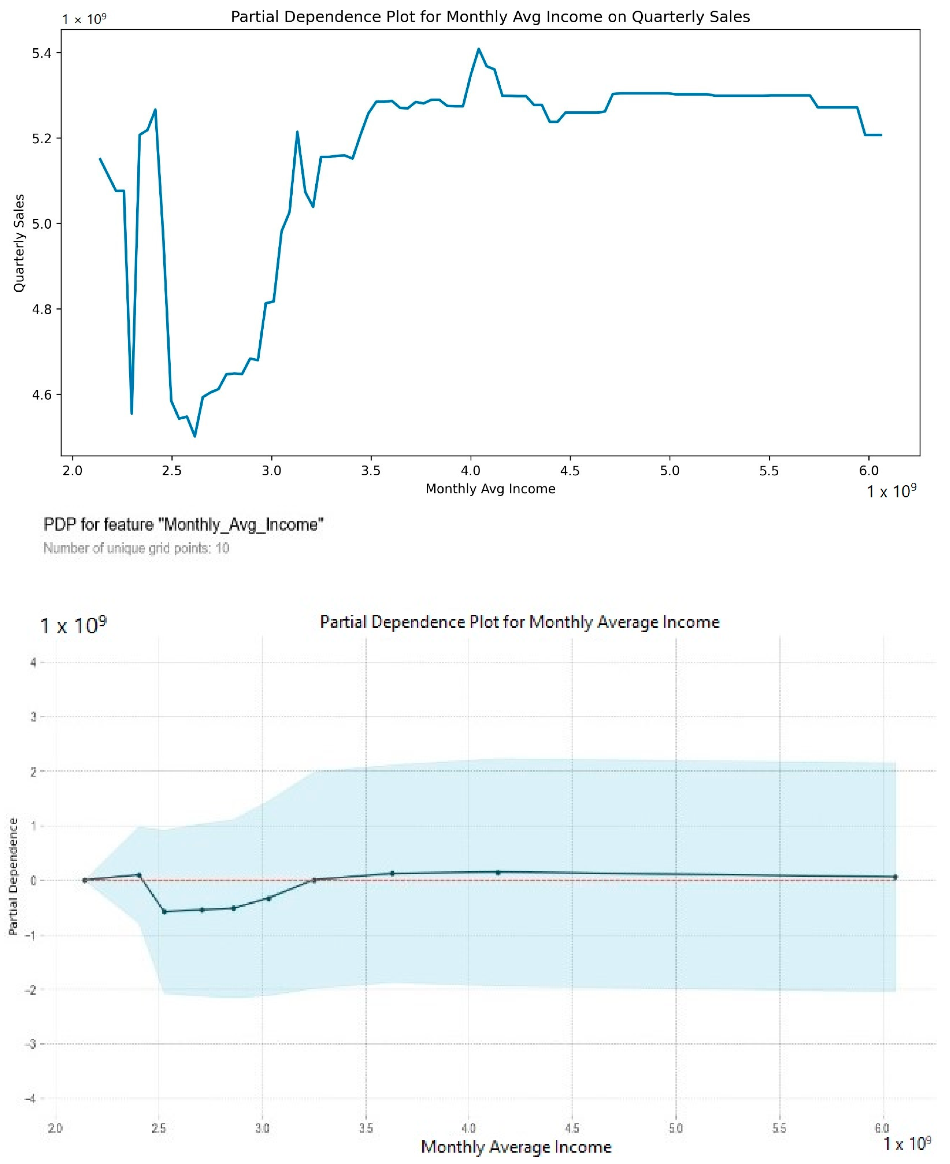
2.4.2. Partial Dependence Plots (PDPs)

In recent years, the field of machine learning has made efforts to create methods for interpreting the inner workings of predictions, which have historically been black boxes [41]. Partial dependence plots (PDPs) are valuable tools for investigating the relationship between a target variable and one or more predictors within a machine learning model. These plots visually illustrate the average reaction of the target variable, taking into account the influence of a specific predictor variable and leaving all other predictors unchanged. In the following equation, PDP (X_i, x) defines the partial dependence of the predictor X_i on a value x. N corresponds to the overall count of instances within the dataset. f (X_i,j, x) denotes the forecast rendered by the model f when the value of feature X_i is adjusted to x in instance j, maintaining the constancy of all other predictors. With the PDPs, data can be analyzed for valuable insights into the joint association of air pollution and income with sales in commercial alleys.

$$PDP\left(X_i,x\right)=\frac{1}{N} {\displaystyle \sum }_{j=1}^{N}f\left(X_{i,j},x\right)$$

(1)

3. Results

3.1. Prediction Performance

After conducting a stepwise regression and exploring the VIF, a total of 28 predictors were selected. The R-squared (R²) values represent the goodness-of-fit of each model, with higher values indicating a better fit. The Mean Squared Error (MSE) values measure the accuracy of the models, with lower values indicating better performance.

Table 3. Comparison of performances of RF, XGB, Catboost, and LightGBM.

	RF		XGB		Catboost		LightGBM
	2018–2019	2020–2021	2018–2019	2020–2021	2018–2019	2020–2021	2018–2019	2020–2021
R2	0.90	0.95	0.92	0.96	0.92	0.96	0.92	0.96
MSE	2.39	1.65	1.86	1.07	1.82	1.15	1.84	1.16

below compares the performances of RF, XGB, Catboost, and LightGBM before COVID-19 (2018–2019) and during the COVID-19 pandemic (2020–2021). Catboost showed the best performance among the four models before COVID-19 (R² = 0.92, MSE = 1.82). During the COVID-19 pandemic, XGB showed the best model fit (R² = 0.96, MSE = 1.15). For further analyses, Catboost was used due to its better performance before COVID-19, which is a normal time period before the pandemic, to explore the association between sales and predictor variables.

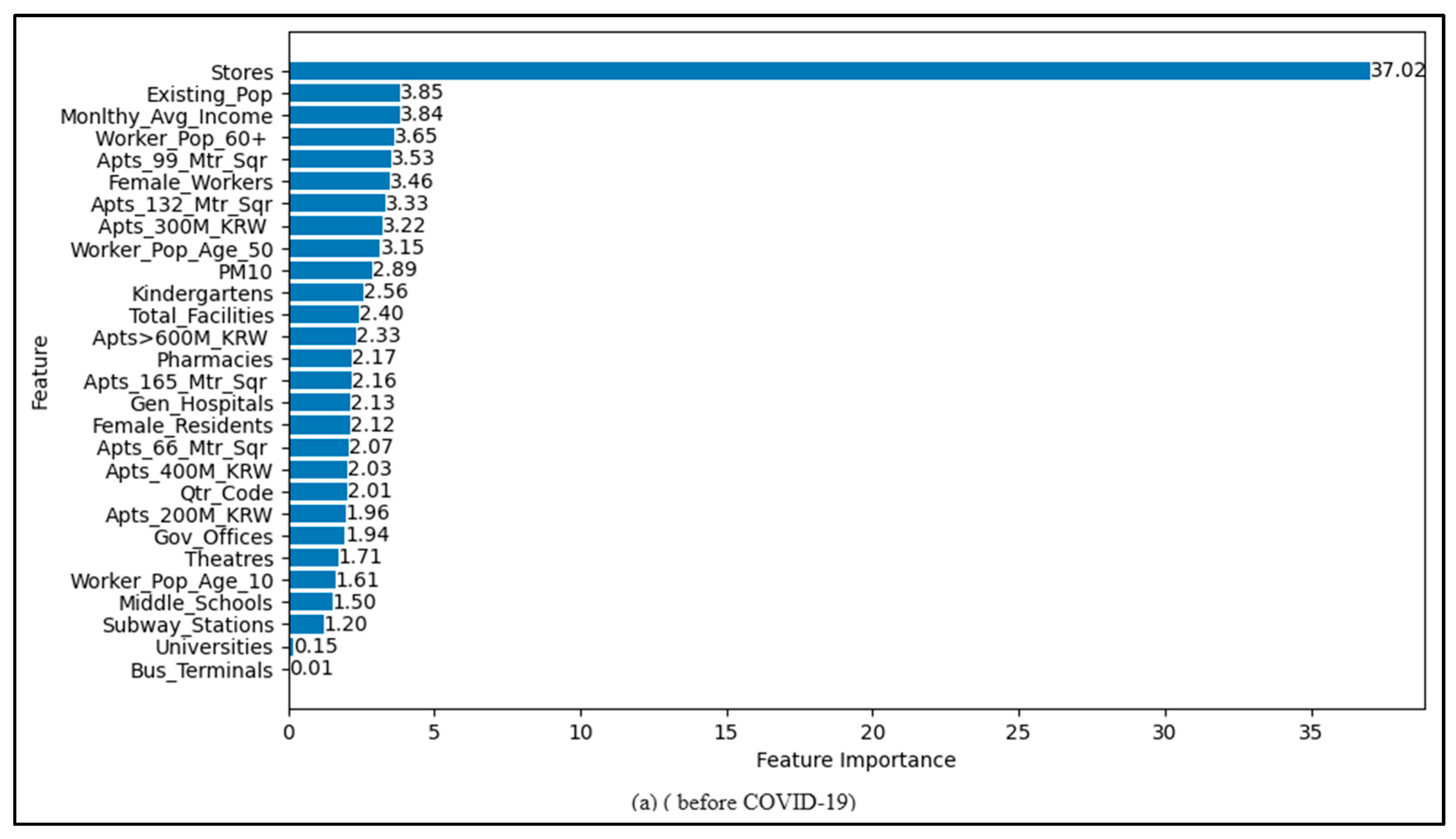
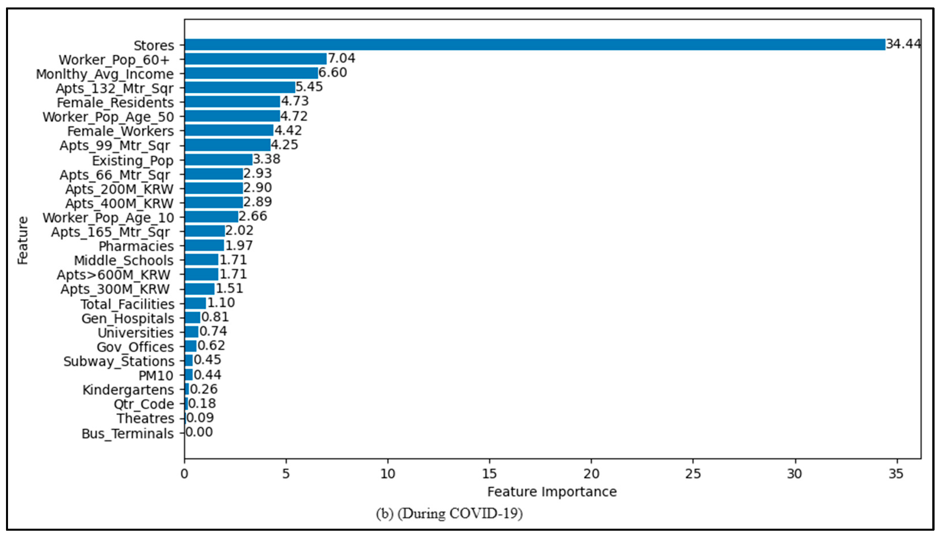
3.2. Importance of Predictor Variables

The relative importance of the selected 28 predictor variables in the prediction of sales is shown in Figure 3a,b. When comparing the relative importance of two critical factors, average monthly salary and PM₁₀, in predicting quarterly sales, there is a notable shift in importance over two different time periods.

Before the onset of the COVID-19 pandemic, both characteristics held positions in the top 10 prominent predictors. Specifically, PM₁₀ ranked as the 10th most important feature, underscoring its relevance to sales forecasting, while average monthly income secured the 3rd position. This indicates that pre-pandemic, the economic factor of monthly income played a substantial role in shaping quarterly sales predictions.

During the COVID-19 pandemic, there were significant changes in what factors were most important for predicting outcomes. Notably, while the importance of monthly average income remained consistent, PM₁₀ experienced a remarkable decline in its relevance. In the pandemic period, PM₁₀ descended to the 24th position among 28 features, illustrating its reduced impact on quarterly sales prediction compared to the pre-pandemic period. This shift underscores the dynamic nature of predictive factors in the context of changing external circumstances. It highlights the influence of the pandemic on consumer behavior, with environmental factors like PM₁₀ giving way to other influential variables in shaping sales trends during and after the COVID-19 crisis.

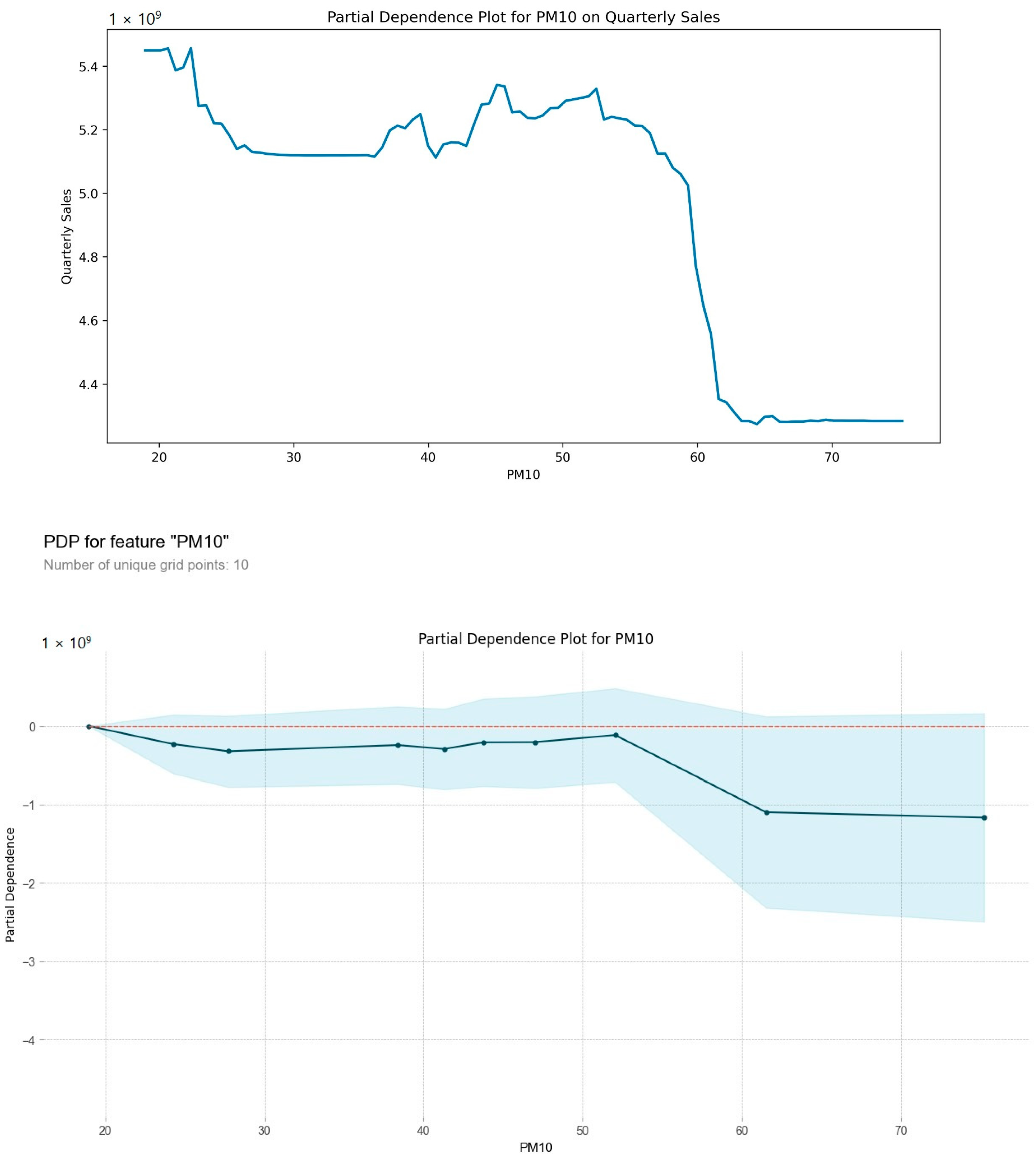
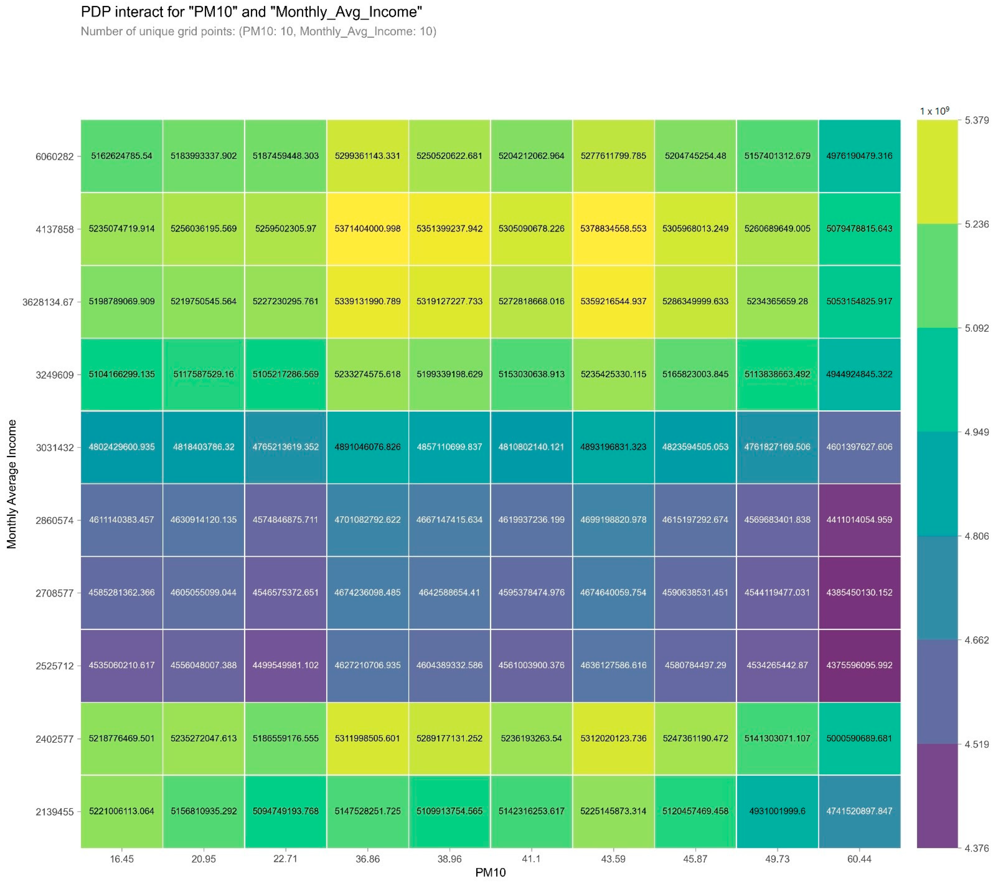
3.3. Joint Association of Air Pollution and Income with Sales

The effect of air pollution on sales forecasts before and during the COVID-19 pandemic is visually presented in Figure 4 and Figure 5. In both periods, a consistent negative relationship between PM₁₀ and quarterly sales was observed.

Before COVID-19, there was an indeterminate decrease in quarterly sales corresponding to an increase in PM₁₀ concentrations. Specifically, there was an approximate decrease of USD 300,000 associated with PM₁₀ levels ranging from 18 to 27 μg/m³, and a more substantial decrease of approximately USD 1,000,000 between PM₁₀ levels of 55 and 62 μg/m³. This can be seen in Figure 4.

During the COVID-19 period, a distinct pattern emerged. There was a significant increase in sales, approximately USD 150,000, as PM₁₀ levels rose from 35 to 38 μg/m³. However, this was followed by a dramatic drop in sales, amounting to USD 300,000, as PM₁₀ levels increased from 38 to 55 μg/m³, as shown in Figure 5. When quarterly sales decrease, PM₁₀ values tend to be higher. This phenomenon highlights the complex and dynamic relationship between air quality and sales during the pandemic, and it is noteworthy that the second drop in sales during 2020–2021 was comparatively smaller than in the pre-pandemic period of 2018–2019. It is evident that higher PM₁₀ values are consistently linked to lower quarterly sales in both time periods.

The associations between monthly salary and sales were examined using PDPs. There were V-shaped relationships between income and sales, although the association was mostly positive after USD 2500. The large drops between incomes of USD 2000 and USD 2500 before and during the COVID-19 pandemic were unexpected. The average monthly income before COVID-19 and during the COVID-19 pandemic seems to have had a positive association in both periods, as visualized in Figure 6 and Figure 7.

The joint association of air pollution (PM₁₀) and the monthly average income with sales is visually presented in Figure 8 and Figure 9, representing the pre-COVID-19 and during the COVID-19 pandemic periods, respectively. These figures provide valuable insights into the dynamics of sales behavior.

A clear pattern emerges in both time periods. The lowest sales (depicted in dark blue) consistently appear within a range of relatively modest income levels, typically around USD 2500, coupled with higher PM₁₀ concentrations in the range of 50 to 75 μg/m³. Conversely, the highest sales (illustrated in yellow) tend to coincide with higher monthly salaries exceeding USD 6000 and lower PM₁₀ values around 16 μg/m³ before COVID-19. This pattern underscores the significant influence of income and air quality on sales outcomes. Importantly, it is evident that individuals with higher income levels living near commercial alleys significantly contribute to increased sales figures, particularly when exposed to lower PM₁₀ levels. This association was notably pronounced before the COVID-19 pandemic. However, a notable transformation occurred during the COVID-19 pandemic. The very lowest sales (depicted in dark blue) persisted across a range of PM₁₀ concentrations, irrespective of income levels. This shift is attributed to a sharp reduction in sales resulting from lockdown measures and social distancing during the pandemic, which indicates that the concentration of PM₁₀ after COVID-19 had no discernible relationship with sales in commercial alleys for individuals with lower income levels. This observation underscores the profound impact of external events, such as the pandemic, in reshaping the dynamics of income, air quality, and sales in commercial areas.

4. Discussion

The findings presented in this study shed light on the dynamic interplay between various predictor variables, specifically PM₁₀, income, and their joint association, in the context of predicting quarterly sales trends. These findings take on added significance in light of the disruptive impact of the COVID-19 pandemic on consumer behavior and economic conditions. While previous studies primarily focused on the impact of weather conditions on sales [42,43,44,45], our investigation highlights the need to consider broader environmental and economic factors, such as PM₁₀ levels and income, as potential drivers of sales trends.

The feature importance analysis revealed a striking shift in the importance of PM₁₀ as a predictor of quarterly sales before and during the COVID-19 pandemic. Pre-pandemic, PM₁₀ ranked as the 10th most important feature, highlighting its importance to sales forecasting [46]. This suggested that, in the absence of external shocks, environmental factors like air quality played a noteworthy role in shaping sales predictions [47]. However, during the pandemic, PM₁₀ experienced a remarkable decline in its importance, plummeting to the 24th position among 28 features [48,49]. This shift underscores the pandemic’s transformative effect on consumer behavior, where factors like air pollution receded in importance compared to other influential variables [38].

The study identified a consistent interesting correlation between PM₁₀ levels and quarterly sales both before and during the COVID-19 pandemic. Notably, pre-pandemic increases in PM₁₀ concentrations corresponded to substantial declines in quarterly sales. This association is a significant finding, highlighting the sensitivity of sales to air quality, with higher levels of PM₁₀ linked to reduced economic performance [50,51]. During the COVID-19 period, the relationship became even more complex. A slight increase in sales was observed; noticeably, PM₁₀ level values were quite low compared to before-pandemic values, followed by a subsequent drop in sales with higher PM₁₀ levels. This dynamic suggests that the pandemic may have influenced consumer behavior, leading to nuanced responses to air quality changes [52,53]. The observation that the second drop in sales during the pandemic was smaller than prior to the pandemic suggests potential adaptation and resilience within the business environment [54,55,56].

The analysis of the association between income and sales revealed intriguing V-shaped relationships, particularly in income ranges between USD 2000 and USD 2500 before and during the COVID-19 pandemic. These unexpected drops in sales within this income bracket warrant further investigation. However, overall, the association between income and sales was predominantly positive, indicating that higher income levels were generally linked to higher quarterly sales. This aligns with economic theory and underscores the importance of disposable income in driving consumer spending [57,58]. The V-shaped patterns suggest that there may be specific income thresholds that significantly impact consumer behavior, which warrants deeper exploration in future studies.

The joint association analysis of PM₁₀ and income before and during the COVID-19 pandemic provides valuable insights into the dynamics of sales behavior. Before COVID-19, individuals with higher income levels and less PM₁₀ exposure were associated with the highest sales figures, emphasizing the significance of both economic and environmental factors [59]. However, during the pandemic, the relationship changed significantly [60]. The lowest sales persisted across a range of PM₁₀ concentrations, irrespective of income levels, highlighting the profound impact of external events, such as lockdowns and social distancing measures [61]. This shift underscores how crises can disrupt traditional patterns, with environmental factors becoming less influential in the face of such extraordinary events. Our analysis indicates that increased air pollution levels correlate with a decrease in sales in commercial alleys. This trend aligns with studies suggesting that consumers tend to reduce outdoor activities and shift toward online shopping in response to poor air quality [62]. For instance, air pollution levels can lead to increased consumer anxiety and a preference for indoor activities, indirectly impacting spending patterns in physical retail spaces [62]. Our findings also reveal that the combined effect of air pollution and income levels plays a significant role in determining expenditure behaviors. This is particularly evident during the COVID-19 pandemic, when shifts in spending habits were observed. High- and lower-income households showed a greater tendency toward irregular spending than before the COVID-19 pandemic. This demonstrates how socioeconomic and environmental factors interplay with external events to influence consumer behavior.

In addition to these key findings, it is essential to recognize that the COVID-19 pandemic served as a catalyst for redefining consumer behavior and business strategies globally. The pandemic prompted businesses to adapt rapidly to new circumstances, with many shifting their focus to e-commerce, contactless services, and remote work [63,64,65]. While air quality remains a critical factor, the pandemic demonstrated that external events could override its influence. Thus, businesses must remain agile and responsive to evolving consumer preferences and external shocks. Considering the risk levels of COVID-19, future research is necessary to conduct an analysis of the relationship, such as how consumers’ consumption behavior has changed.

5. Conclusions

This study investigated the relative importance of monthly income and air pollution in predicting sales in commercial alleys and the joint association of monthly income and air pollution with sales. Catboost was selected as the best algorithm for the analyses using machine learning techniques. This study underscored the importance of adaptability in predictive models, especially in the face of external shocks such as the COVID-19 pandemic.

It is important to note several limitations of this study. Firstly, the data used for the analysis was limited to a specific region and time period. The extrapolation of these findings to other regions or different time frames should be undertaken with caution, as variations in consumer behavior, economic conditions, and environmental factors may significantly impact the results. Additionally, while this study examined a comprehensive set of predictor variables, there may be other unaccounted-for factors influencing sales trends that require further investigation. Furthermore, causal relationships between predictor variables and sales were not established in this study, and future research should delve into causality. Lastly, the V-shaped income–sales relationships observed warrant a more in-depth investigation to understand the underlying mechanisms and their generalizability. The results highlight the shifting significance of predictor variables, such as PM₁₀ and income, and emphasize the need for dynamic modeling to capture changing consumer behavior. Understanding these dynamics can be invaluable for businesses and policy makers seeking to navigate and respond effectively to evolving economic and environmental conditions.

Our study provides indirect yet insightful evidence of changing patterns of consumer behavior, influenced by both environmental factors, such as air pollution, and socioeconomic factors, like income. These findings are particularly relevant in the context of urban sustainability and planning. They highlight the need for cities to consider environmental health and its impact on economic activity within urban commercial spaces. The shift toward online shopping in response to poor air quality and the varied spending habits based on income levels during the pandemic offer valuable insight for policy makers and business owners. Future urban planning and economic strategies should integrate these behavioral insights to promote sustainable and resilient urban commercial environments.

References

1. Liao, S.; Liu, K.; Yang, Y.; Liu, Y. The Correlation between Convenience Stores’ Distribution and Urban Spatial Function: Taking the FamilyMart Stores in Shanghai as an Example. Sustainability 2022, 14, 9457. [Google Scholar] [CrossRef]
2. Sobolevsky, S.; Sitko, I.; Tachet des Combes, R.; Hawelka, B.; Murillo Arias, J.; Ratti, C. Cities through the prism of people’s spending behavior. PLoS ONE 2016, 11, e0146291. [Google Scholar] [CrossRef] [PubMed]
3. Carpio-Pinedo, J.; Romanillos, G.; Aparicio, D.; Martín-Caro, M.S.H.; García-Palomares, J.C.; Gutiérrez, J. Towards a new urban geography of expenditure: Using bank card transactions data to analyze multi-sector spatiotemporal distributions. Cities 2022, 131, 103894. [Google Scholar] [CrossRef]
4. Phipps, S.A.; Burton, P.S. What’s mine is yours? The influence of male and female incomes on patterns of household expenditure. Economica 1998, 65, 599–613. [Google Scholar] [CrossRef]
5. Williams, A.M. Understanding the micro-determinants of defensive behaviors against pollution. Ecol. Econ. 2019, 163, 42–51. [Google Scholar] [CrossRef]
6. Ellison, B.; McFadden, B.; Rickard, B.J.; Wilson, N.L. Examining food purchase behavior and food values during the COVID-19 pandemic. Appl. Econ. Perspect. Policy 2021, 43, 58–72. [Google Scholar] [CrossRef]
7. Alatrista-Salas, H.; Gauthier, V.; Nunez-del-Prado, M.; Becker, M. Impact of natural disasters on consumer behavior: Case of the 2017 El Niño phenomenon in Peru. PLoS ONE 2021, 16, e0244409. [Google Scholar] [CrossRef] [PubMed]
8. Carpio-Pinedo, J.; Gutiérrez, J. Consumption and symbolic capital in the metropolitan space: Integrating ‘old’ retail data sources with social big data. Cities 2020, 106, 102859. [Google Scholar] [CrossRef]
9. Bachas, N.; Ganong, P.; Noel, P.J.; Vavra, J.S.; Wong, A.; Farrell, D.; Greig, F.E. Initial Impacts of the Pandemic on Consumer Behavior: Evidence from Linked Income, Spending, and Savings Data; No. w27617; National Bureau of Economic Research: Cambridge, MA, USA, 2020. [Google Scholar]
10. Baker, S.R.; Farrokhnia, R.A.; Meyer, S.; Pagel, M.; Yannelis, C. How does household spending respond to an epidemic? Consumption during the 2020 COVID-19 pandemic. Rev. Asset Pricing Stud. 2020, 10, 834–862. [Google Scholar] [CrossRef]
11. Bresnahan, B.W.; Dickie, M.; Gerking, S. Averting behavior and urban air pollution. Land Econ. 1997, 73, 340–357. [Google Scholar] [CrossRef]
12. Bujisic, M.; Bogicevic, V.; Parsa, H.G. The effect of weather factors on restaurant sales. J. Foodserv. Bus. Res. 2017, 20, 350–370. [Google Scholar] [CrossRef]
13. Liu, L.; Fang, J.; Li, M.; Hossin, M.A.; Shao, Y. The effect of air pollution on consumer decision making: A review. Clean. Eng. Technol. 2022, 9, 100514. [Google Scholar] [CrossRef]
14. Bartik, T.J. Evaluating the benefits of non-marginal reductions in pollution using information on defensive expenditures. J. Environ. Econ. Manag. 1988, 15, 111–127. [Google Scholar] [CrossRef]
15. Shahin Sharifi, S. Impacts of the trilogy of emotion on future purchase intentions in products of high involvement under the mediating role of brand awareness. Eur. Bus. Rev. 2014, 26, 43–63. [Google Scholar] [CrossRef]
16. Barwick, P.J.; Li, S.; Rao, D.; Zahur, N.B. The morbidity cost of air pollution: Evidence from consumer spending in China. SSRN 2018, 2999068. [Google Scholar]
17. Chang, K.H.; Hsu, P.Y.; Lin, C.J.; Lin, C.L.; Juo, S.H.H.; Liang, C.L. Traffic-related air pollutants increase the risk for age-related macular degeneration. J. Investig. Med. 2019, 67, 1076–1081. [Google Scholar] [CrossRef]
18. Sun, X. Air Pollution and Avoidance Behavior: Evidence from Leisure Activities in the US. SSRN 2023, 4570602. [Google Scholar] [CrossRef]
19. Keiser, D.; Lade, G.; Rudik, I. Air pollution and visitation at US national parks. Sci. Adv. 2018, 4, eaat1613. [Google Scholar] [CrossRef]
20. Chen, C.M.; Lin, Y.L.; Hsu, C.L. Does air pollution drive away tourists? A case study of the Sun Moon Lake National Scenic Area, Taiwan. Transp. Res. Part D Transp. Environ. 2017, 53, 398–402. [Google Scholar] [CrossRef]
21. Jung, H. Economic effects of ambient air pollution on consumer shopping behaviors. Econ. Bus. Lett. 2020, 9, 255–264. [Google Scholar] [CrossRef]
22. Qiu, Q.; Wang, Y.; Qiao, S.; Liu, R.; Bian, Z.; Yao, T.; Nguyen, T.S. Does air pollution affect consumer online purchasing behavior? The effect of environmental psychology and evidence from China. J. Clean. Prod. 2020, 260, 120795. [Google Scholar] [CrossRef]
23. Xu, G.; Feng, X.; Li, Y.; Jia, J. Mediation effects of online public attention on the relationship between air pollution and precautionary behavior. J. Manag. Sci. Eng. 2021, 7, 159–172. [Google Scholar] [CrossRef]
24. Liu, J.; Zou, P.; Ma, Y. The Effect of Air Pollution on Food Preferences. J. Acad. Mark. Sci. 2021, 50, 410–423. [Google Scholar] [CrossRef]
25. Das, D.; Sarkar, A.; Debroy, A. Impact of COVID-19 on changing consumer behaviour: Lessons from an emerging economy. Int. J. Consum. Stud. 2022, 46, 692–715. [Google Scholar] [CrossRef]
26. Valaskova, K.; Durana, P.; Adamko, P. Changes in consumers’ purchase patterns as a consequence of the COVID-19 pandemic. Mathematics 2021, 9, 1788. [Google Scholar] [CrossRef]
27. Milfont, T.L.; Markowitz, E. Sustainable consumer behavior: A multilevel perspective. Curr. Opin. Psychol. 2016, 10, 112–117. [Google Scholar] [CrossRef]
28. Ahmed, M.E.; Khan, M.M.; Samad, N. Income, social class and consumer behaviour: A focus on developing nations. J. Appl. Bus. Econ. Res. 2016, 14, 6679–6702. [Google Scholar]
29. Delibasic, B.; Vukicevic, M.; Jovanovic, M.I.L.O. White-box decision tree algorithms: A pilot study on perceived usefulness, perceived ease of use, and perceived understanding. Int. J. Eng. Educ. 2013, 29, 674–687. [Google Scholar]
30. Gulati, P.; Sharma, A.; Gupta, M. Theoretical study of decision tree algorithms to identify pivotal factors for performance improvement: A review. Int. J. Comput. Appl. 2016, 141, 19–25. [Google Scholar] [CrossRef]
31. Herm, L.V.; Heinrich, K.; Wanner, J.; Janiesch, C. Stop ordering machine learning algorithms by their explainability! A user-centered investigation of performance and explainability. Int. J. Inf. Manag. 2023, 69, 102538. [Google Scholar] [CrossRef]
32. Pintelas, E.; Livieris, I.E.; Pintelas, P. A grey-box ensemble model exploiting black-box accuracy and white-box intrinsic interpretability. Algorithms 2020, 13, 17. [Google Scholar] [CrossRef]
33. Kim, M.; Kim, G. Modeling and Predicting Urban Expansion in South Korea Using Explainable Artificial Intelligence (XAI) Model. Appl. Sci. 2022, 12, 9169. [Google Scholar] [CrossRef]
34. Kang, J.Y.; Lee, S. Exploring food deserts in Seoul, South Korea during the COVID-19 pandemic (from 2019 to 2021). Sustainability 2022, 14, 5210. [Google Scholar] [CrossRef]
35. Uchiyama, Y.; Kohsaka, R. Access and use of green areas during the covid-19 pandemic: Green infrastructure management in the “new normal”. Sustainability 2020, 12, 9842. [Google Scholar] [CrossRef]
36. Bounie, D.; Camara, Y.; Galbraith, J.W. Consumers’ mobility, expenditure and online-offline substitution response to COVID-19: Evidence from French transaction data. SSRN 2022, 3588373. [Google Scholar] [CrossRef]
37. Khan, J.R.; Awan, N.; Islam, M.M.; Muurlink, O. Healthcare capacity, health expenditure, and civil society as predictors of COVID-19 case fatalities: A global analysis. Front. Public Health 2020, 8, 347. [Google Scholar] [CrossRef]
38. Di Crosta, A.; Ceccato, I.; Marchetti, D.; La Malva, P.; Maiella, R.; Cannito, L.; Di Domenico, A. Psychological factors and consumer behavior during the COVID-19 pandemic. PLoS ONE 2021, 16, e0256095. [Google Scholar] [CrossRef]
39. Son, J.Y.; Bell, M.L.; Lee, J.T. Individual exposure to air pollution and lung function in Korea: Spatial analysis using multiple exposure approaches. Environ. Res. 2010, 110, 739–749. [Google Scholar] [CrossRef]
40. O’brien, R.M. A caution regarding rules of thumb for variance inflation factors. Qual. Quant. 2007, 41, 673–690. [Google Scholar] [CrossRef]
41. Carvalho, D.V.; Pereira, E.M.; Cardoso, J.S. Machine Learning Interpretability: A Survey on Methods and Metrics. Electronics 2019, 8, 832. [Google Scholar] [CrossRef]
42. Steele, A.T. Weather’s Effect on the Sales of a Department Store. J. Mark. 1951, 15, 436–443. [Google Scholar] [CrossRef]
43. Maunder, W.J. Weekly weather and economic activities on a national scale: An example using United States retail trade data. Weather 1973, 28, 2–19. [Google Scholar] [CrossRef]
44. Starr, M. The effects of weather on retail sales. SSRN 2000, 221728. [Google Scholar]
45. Bertrand, J.L.; Brusset, X.; Fortin, M. Assessing and hedging the cost of unseasonal weather: Case of the apparel sector. Eur. J. Oper. Res. 2015, 244, 261–276. [Google Scholar] [CrossRef]
46. Jung, H. The impact of ambient fine particulate matter on consumer expenditures. Sustainability 2020, 12, 1855. [Google Scholar] [CrossRef]
47. Kang, H.; Suh, H.; Yu, J. Does air pollution affect consumption behavior? Evidence from Korean retail sales. Asian Econ. J. 2019, 33, 235–251. [Google Scholar] [CrossRef]
48. Seo, J.H.; Kim, J.S.; Yang, J.; Yun, H.; Roh, M.; Kim, J.W.; Yu, S.; Na Jeong, N.; Jeon, H.W.; Choi, J.S.; et al. Changes in Air Quality during the COVID-19 Pandemic and Associated Health Benefits in Korea. Appl. Sci. 2020, 10, 8720. [Google Scholar] [CrossRef]
49. Akan, A.P.; Coccia, M. Changes of air pollution between countries because of lockdowns to face COVID-19 pandemic. Appl. Sci. 2022, 12, 12806. [Google Scholar] [CrossRef]
50. Tschofen, P.; Azevedo, I.L.; Muller, N.Z. Fine particulate matter damages and value added in the US economy. Proc. Natl. Acad. Sci. USA 2019, 116, 19857–19862. [Google Scholar] [CrossRef]
51. Yoon, H. Effects of particulate matter (PM10) on tourism sales revenue: A generalized additive modeling approach. Tour. Manag. 2019, 74, 358–369. [Google Scholar] [CrossRef]
52. Cai, L.; Yuen, K.F.; Fang, M.; Wang, X. A literature review on the impact of the COVID-19 pandemic on consumer behaviour: Implications for consumer-centric logistics. Asia Pac. J. Mark. Logist. 2023, 35, 2682–2703. [Google Scholar] [CrossRef]
53. Safara, F. A computational model to predict consumer behaviour during COVID-19 pandemic. Comput. Econ. 2022, 59, 1525–1538. [Google Scholar] [CrossRef] [PubMed]
54. Mehta, S.; Saxena, T.; Purohit, N. The new consumer behaviour paradigm amid COVID-19: Permanent or transient? J. Health Manag. 2020, 22, 291–301. [Google Scholar] [CrossRef]
55. Jo, H.; Shin, E.; Kim, H. Changes in consumer behaviour in the post-COVID-19 era in Seoul, South Korea. Sustainability 2020, 13, 136. [Google Scholar] [CrossRef]
56. Tien, N.H.; Ngoc, N.M.; Anh, D.B.H. Change of consumer behavior in the post COVID-19 period. Change 2021, 2, 53. [Google Scholar]
57. Dossche, M.; Forsells, M.; Rossi, L.; Stoevsky, G. Private consumption and its drivers in the current economic expansion. Econ. Bull. Artic. 2018, 5. [Google Scholar]
58. Khari, P. Economic Productivity through Net National Disposable Income. J. Bus. Manag. Inf. Syst. 2023, 10, 1–7. [Google Scholar] [CrossRef]
59. Lenzen, M.; Li, M.; Malik, A.; Pomponi, F.; Sun, Y.Y.; Wiedmann, T.; Faturay, F.; Fry, J.; Gallego, B.; Geschke, A.; et al. Global socio-economic losses and environmental gains from the Coronavirus pandemic. PLoS ONE 2020, 15, e0235654. [Google Scholar] [CrossRef]
60. Jung, H.; Kim, J.H.; Hong, G. Impacts of the COVID-19 crisis on single-person households in South Korea. J. Asian Econ. 2023, 84, 101557. [Google Scholar] [CrossRef]
61. Verhoef, P.C.; Noordhoff, C.S.; Sloot, L. Reflections and predictions on effects of COVID-19 pandemic on retailing. J. Serv. Manag. 2023, 34, 274–293. [Google Scholar] [CrossRef]
62. Liang, J.; Ma, J.; Zhu, J.; Jin, X. Online or Offline? How Smog Pollution Affects Customer Channel Choice for Purchasing Fresh Food. Front. Psychol. 2021, 12, 682981. [Google Scholar] [CrossRef] [PubMed]
63. Ferreira, R.; Pereira, R.; Bianchi, I.S.; da Silva, M.M. Decision factors for remote work adoption: Advantages, disadvantages, driving forces and challenges. J. Open Innov. Technol. Mark. Complex. 2021, 7, 70. [Google Scholar] [CrossRef]
64. Ng, P.M.; Lit, K.K.; Cheung, C.T. Remote work as a new normal? The technology-organization-environment (TOE) context. Technol. Soc. 2022, 70, 102022. [Google Scholar] [CrossRef] [PubMed]
65. Atobishi, T.; Nosratabadi, S. Drivers and constraints of employee satisfaction with remote work: An empirical analysis. Organizacija 2023, 56, 93–105. [Google Scholar] [CrossRef]
Figure 1. Workflow of this study.
Sustainability 16 00530 g001
Figure 2. Commercial alleys in Seoul.
Sustainability 16 00530 g002
Figure 3. Importance of influential factors for the CatBoost model. Sales_Amount: quarterly total sales amount; Stores: number of stores; Worker_Pop_60+: population of workers aged 60 and above; Qtr_Code: quarter code; Gen_Hospitals: number of general hospitals; Subway_Stations: number of subway stations; Apts>600M_KRW: number of apartments priced KRW 600 million and above; Apts_300M_KRW: number of apartments priced KRW 300 million; Female_Residents: female resident population; Existing_Pop: female population; Apts_132_Mtr_Sq: number of apartments with an area of 132 m2; Total_Facilities: number of attracting facilities; Female_Workers: female worker population; Worker_Pop_Age_10: population of workers aged 10; Bus_Terminals: number of bus terminals; Middle_Schools: number of middle schools; PM10: particulate matter with diameter of 10 (PM); Theatres: number of theatres; Monthly_Avg_Income: monthly average income amount; Kindergartens: number of kindergartens; Apts_66_Mtr_Sqr: number of apartments with an area of 66 m2; Universities: number of universities; Worker_Pop_Age_50: population of workers aged 50; Gov_Offices: number of government offices; Pharmacies: number of pharmacies; Apts_400M_KRW: number of apartments priced KRW 400 million; Apts_200M_KRW: number of apartments priced KRW 200 million; Apts_99_Mtr_Sqr: number of apartments with an area of 99 m2; Apts_165_Mtr_Sqr: number of apartments with an area of 165 m2.
Sustainability 16 00530 g003aSustainability 16 00530 g003b
Figure 4. Partial dependence of PM10 on quarterly sales before COVID-19 (2018–2019).
Sustainability 16 00530 g004
Figure 5. Partial dependence of PM10 on quarterly sales during the COVID-19 pandemic (2020–2021).
Sustainability 16 00530 g005
Figure 6. Partial dependence of monthly average income on quarterly sales before COVID-19 (2018–2019).
Sustainability 16 00530 g006
Figure 7. Partial dependence of monthly average income on quarterly sales during the COVID-19 pandemic (2020–2021).
Sustainability 16 00530 g007
Figure 8. Joint association of PM10 and monthly average income with sales before COVID-19 (2018–2019).
Sustainability 16 00530 g008
Figure 9. Joint association of PM10 and monthly average income on sales during the COVID-19 pandemic (2020–2021).
Sustainability 16 00530 g009