How Did Urban Environmental Characteristics Influence Land Surface Temperature in Hong Kong from 2017 to 2022? Evidence from Remote Sensing and Land Use Data

Abstract

Urbanization has led to environmental challenges, with the urban heat island effect being a prominent concern. Understanding the influence of urban environmental characteristics (UECs) on land surface temperature (LST) is essential for addressing this issue and promoting sustainable urban development. The spatiotemporal characteristics and influencing factors of LST have been investigated in past studies, but research that explicitly investigates the key factors and long-term spatial relationships affecting LST in city-scale urban areas is limited. Remote sensing techniques provide valuable insights into LST patterns and the relationship between urban environment and temperature dynamics. We utilized Landsat 8 images to derive the LST and six spectral indices from 2017 to 2022 in Hong Kong, a city characterized by high population density and rapid urban growth. We also acquired land use data to reflect Hong Kong’s dynamic urban landscape. The complex interactions between urban environment and LST were analyzed using various analytical techniques, including slope trend analysis, land use change detection, and correlation analysis. Finally, we constructed a random forest model to assess the importance of each environmental characteristic. Our findings provide three key insights for regions experiencing rapid urbanization. First, the LST showed an increasing trend in Hong Kong from 2017 to 2022, with the annual LST rising from 21.13 °C to 23.46 °C. Second, we identify negative relationships between LST and vegetation (−0.49)/water bodies (−0.49) and a positive correlation between LST and built-up areas (0.56) utilizing Pearson’s correlation. Third, the dominant influence of built-up areas was underscored, contributing as much as 53.4% to elevated LST levels, with specific attention to the substantial reclamation activities in Hong Kong. The insights from this study provide valuable guidance for policymakers, urban planners, and environmental researchers to formulate evidence-based strategies to achieve a resilient, livable urban future.

1. Introduction

Urbanization is a prominent global trend characterized by rapid population growth and excessive expansion of urban areas [1,2,3]. However, this process may adversely affect urban environments [4,5]. One negative impact is the UHI effect: when urban areas experience higher LST than the surrounding rural areas [6]. This research topic has garnered significant attention. In addition to influencing local climates and posing health risks related to heat [7], the UHI effect contributes to global problems, including global warming [8,9], sea level rise [10,11], and intensification of storms [12,13]. Moreover, when a heatwave occurs in an urban area already experiencing the UHI effect, it can create extreme heat conditions that may potentially induce natural disasters like wildfires or droughts and result in substantial socioeconomic losses [14,15]. Hence, research on analyzing LST patterns and mitigating the UHI effect would provide valuable insights and recommendations for attaining the United Nations Sustainable Development Goals and ensuring a resilient urban future.

Remote sensing is widely recognized as an advanced monitoring technology that offers numerous advantages for studying and analyzing various aspects of the earth’s surface [16]. A key strength of remote sensing is its ability to provide large-scale and long-term monitoring, which allows the retrieval of surface temperature over vast regions and facilitates the study of thermal patterns and dynamics [17]. For example, Kachar et al. [18] used Landsat 7 and Landsat 8 satellite images to generate the spatiotemporal distribution of LST in Tehran from 1999 to 2014. Likewise, Taloor et al. [19] estimated the LST in the Ravi River Basin from February to March 2018 using Landsat 8 satellite imagery. In addition to its application in large-area thermal analysis, remote sensing plays a significant role in characterizing urban environment [20]. Remote sensing plays a significant role in characterizing urban morphology [21,22]. Remote sensing-derived spectral indices such as the NDVI and NDBI serve as valuable indicators of vegetation cover and built-up areas, respectively [23,24]. Furthermore, land use classification allows for the identification and categorization of different land use categories within urban areas, thereby aiding in the assessment of urban morphology and contributing to urban planning efforts [25,26]. These remote sensing products provide a solid foundation for comprehensive urban environmental monitoring.

Studies have validated the benefits of using UECs to analyze LST. One research direction involves exploring the correlation between LST and spectral indices derived from remote sensing data. The relationship between LST and spectral indices was first investigated in East Texas in 1990 [27], and subsequent research further examined this connection. Ref. [28] discussed the relationship between vegetation and LST in North America using NDVI data from 1996 to 2000. The NDBI was employed to study the UHI effect in Hong Kong by using Landsat thermal infrared data [29]. Several studies have investigated the effect of UHIs by combining various spectral indices. For instance, Guha et al. [30] focused on determining the relationship between the estimated LST, NDVI, and NDBI for Florence and Naples, Italy, by using Landsat 8 data. Akher et al. [31] also discovered that the rapid urbanization process in Kolkata contributed to increased LST by using NDVI and NDBI monitoring.

Another direction evaluates LST and its association with land use types, such as vegetation, water bodies, and built-up areas. These studies are crucial for understanding urban heat dynamics and evaluating the effects of landcover changes [32,33]. Exploration of the relationship between urban temperature and land use type began as early as the 1990s in the United States [34]. Research has continued to investigate the influence of land use on LST, considering single and multiple land use types. For instance, Estoque et al. [35] examined the relationship between LST and the spatial patterns of impervious surfaces and greenspaces in the metropolitan areas of Bangkok (Thailand), Jakarta (Indonesia), and Manila (Philippines). Similarly, Jia et al. [36] examined the patterns of LST and landcover in Hong Kong and observed a significant cooling effect of vegetation cover on LST.

Studies have primarily explored the relationship between LST and UECs by using statistical approaches, including the Pearson coefficient, Spearman correlation, and ordinary least squares methods [20,37,38]. However, these methods have limitations in capturing spatial variations because they provide non-spatialized results [39]. In overcoming this limitation, spatial analysis techniques, including spatial bivariate Moran’s I and GWR, have been used [40]. For example, spatial bivariate Moran’s I was used in Phoenix, Arizona, to explore the relationship between vegetation cover and seasonal surface temperature [41]. Moreover, Kashki et al. [42] employed a GWR model to explore the dynamics of LST in response to geographical parameters in Shiraz City, Iran, during the summer of 2019. With the rapid development of artificial intelligence, the attention to data-driven machine and deep learning models is increasing. Random forest is a machine learning algorithm that constructs an ensemble of decision trees using a random selection of observations and covariates [43,44,45]. Its ability to manage complex relationships and capture nonlinear patterns makes it particularly suitable for analyzing the intricate interactions between urban environment and LST.

In this study, we examined the spatiotemporal pattern of LST and explored its relationship with UECs. Our analysis encompassed two categories of UECs: remote sensing spectral indices and land use types. First, we extracted LST and six spectral indices of Hong Kong from 2017 to 2022 from Landsat 8 data on the GEE. To comprehend the spatial and temporal patterns of LST and UECs, we employed Sen’s slope trend analysis and land use change detection. Furthermore, we conducted Pearson correlation and spatial cross-correlation analyses to validate the relationship between LST and UECs. To deepen the analysis, we employed a random forest regression method to evaluate the relative importance of each UEC in relation to LST. This approach enabled us to identify the key drivers influencing LST. Finally, we conducted further analysis of representative UHI areas, with a specific focus on HKIA, to provide recommendations and insights for decision-makers in policy and urban planning.

This paper comprises six sections. Section 2 introduces the study area and data used. Section 3 describes the analytical methods used, and Section 4 presents the results. Next, we analyze the LST mechanism in representative areas and offer recommendations in Section 5. Finally, Section 6 concludes and summarizes the key findings.

2. Study Area and Data

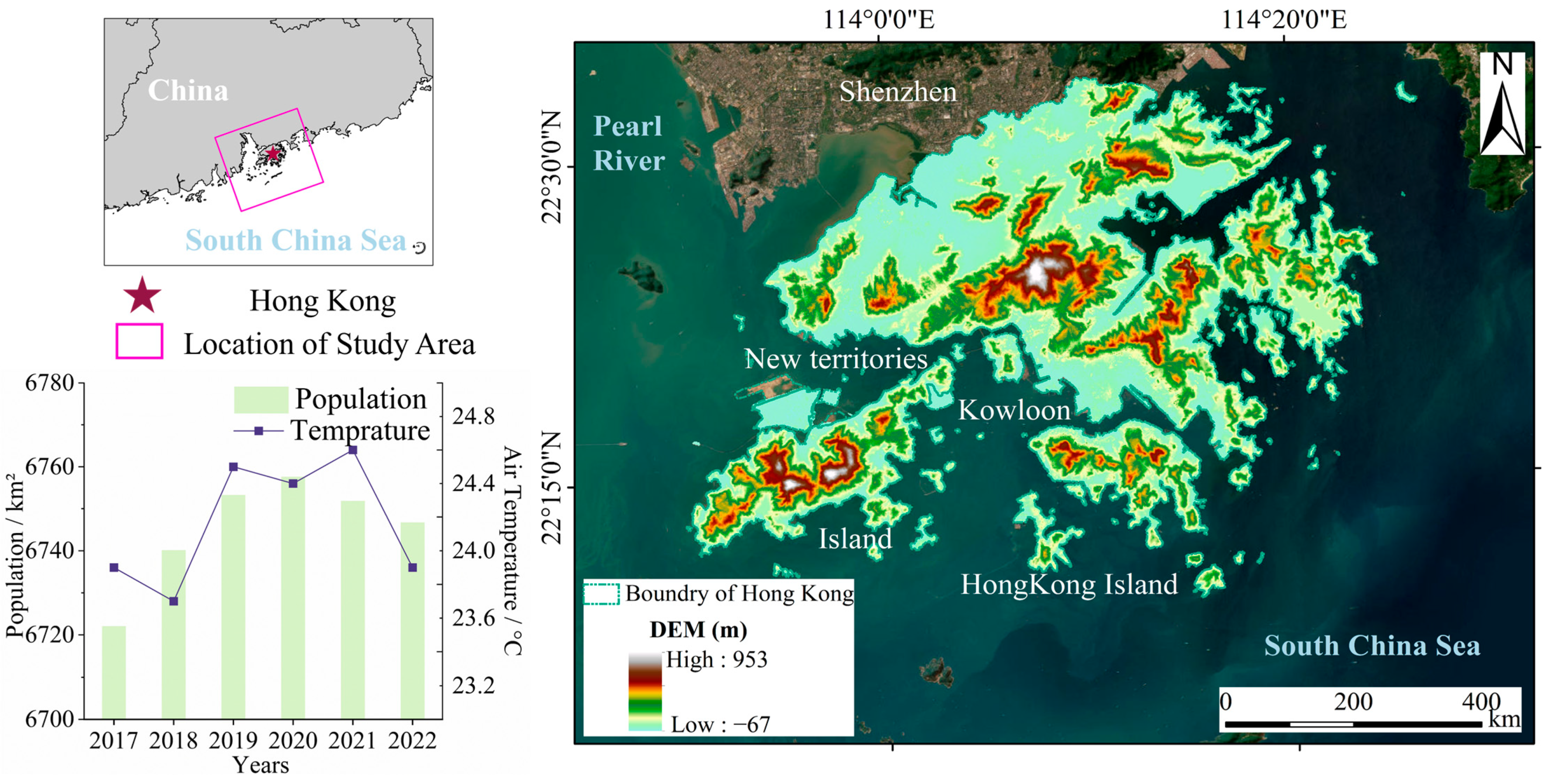
2.1. Study Area

Hong Kong is situated at the mouth of the Pearl River, bordering Shenzhen to the north and the South China Sea to the south. The territory of Hong Kong consists of a main peninsula and a collection of over 260 islands, covering a total land area of approximately 1106 km². The topography of Hong Kong is characterized by hilly and mountainous terrain, with an average elevation of 479 m. In the northern part of Hong Kong, there are lowland areas. Notably, a substantial portion of land in Hong Kong, particularly on Hong Kong Island and the Kowloon Peninsula, has undergone reclamation activities [46]. Its geographic location grants it strategic significance as a central international financial hub and crucial gateway to mainland China. This territory’s unique blend of urban development and natural landscapes offers an excellent context for studying various environmental phenomena.

The climate of Hong Kong is subtropical and influenced by the East Asian Monsoon. Summers are hot, humid, and characterized by frequent rainstorms. Winters are generally mild. The average temperature in Hong Kong from 2017 to 2022 was 24.16 °C. In winter, the low temperature is approximately 10 °C. In summer, the high temperature is approximately 33 °C. This region has distinct wet and dry seasons, with most precipitation occurring from April to September. Regarding socioeconomic conditions, Hong Kong is one of the world’s largest financial hubs because it is the most liberal economic entity in China [47]. Furthermore, as shown in Figure 1, the average population density in Hong Kong from 2017 to 2022 was 6745 persons/km². This means that Hong Kong is one of the most densely populated regions worldwide.

Owing to its exceptional geographical and socioeconomic conditions, the limited space in Hong Kong has resulted in high-density urban development. Because of the significant gap between urban and rural areas, Hong Kong is the one of the most suitable cities for studying the UHI effect.

2.2. UECs

2.2.1. Remote Sensing Data

Landsat 8, launched by NASA and the United States Geological Survey in 2013, is a satellite sensor that provides valuable Earth observation data for various applications. It has a spatial resolution of 30 m for visible, near-infrared, and short-wavelength infrared bands. Landsat 8 thermal infrared bands used to map LST are initially captured at a 100 m resolution and subsequently resampled to a 30 m resolution by data supplier to match the resolution of the remaining bands. This high resolution allows the analysis of large-scale landscape patterns and the identification of various land features. A total of 149 images acquired from 2017 to 2022 were used to capture LST and remote sensing indices in this study.

2.2.2. Land Use Data

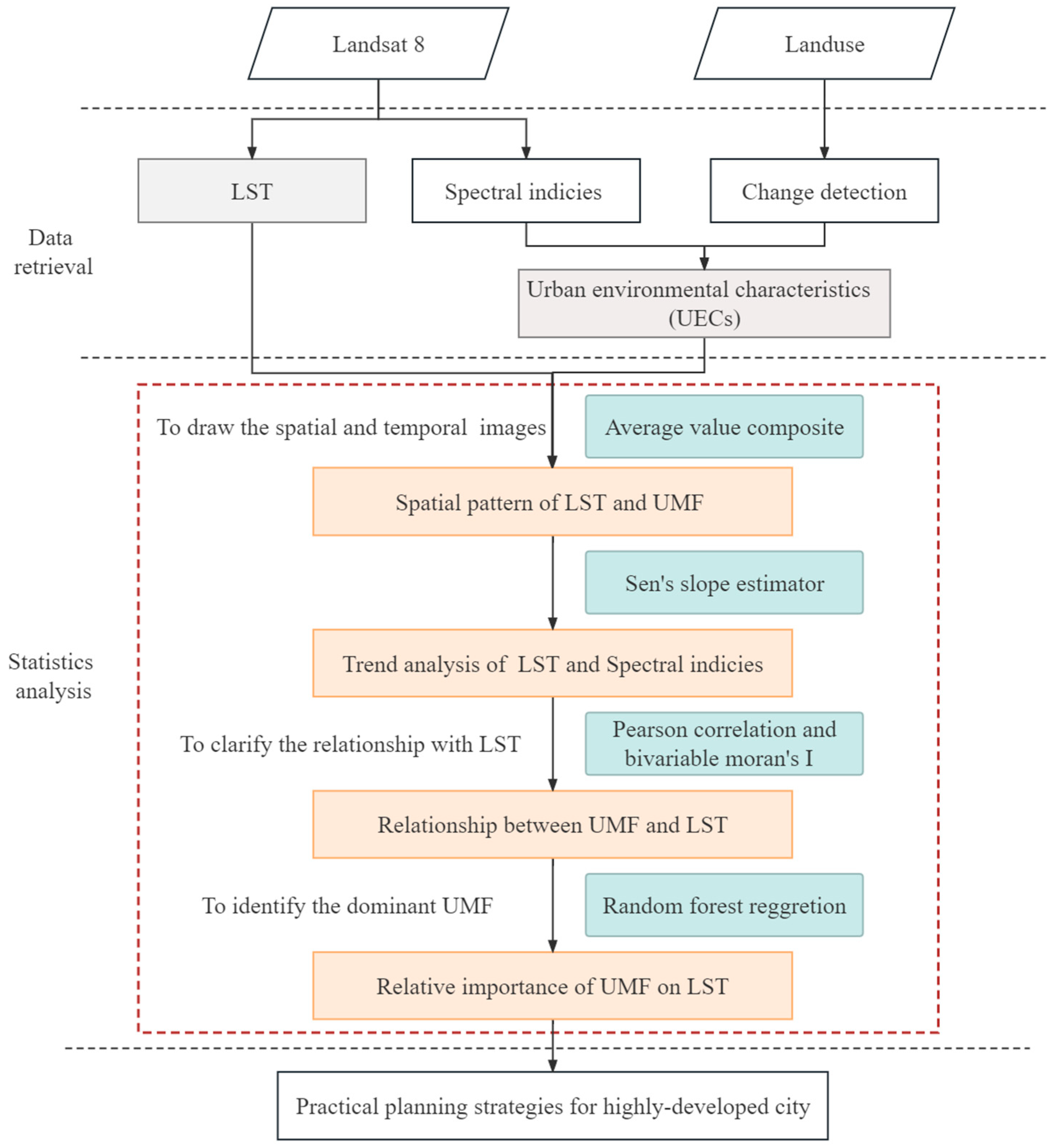
The land use data used in this study were provided by the Data Center for Resources and Environmental Sciences of the Chinese Academy of Science. The dataset used included two periods, 2018 and 2020, corresponding to the earlier and later periods of the study period, respectively [48]. The dataset comprised thematic land use data constructed by manual visual interpretation using remote sensing images from Landsat satellites as the main body. The second classification was divided into 25 categories according to the natural attributes of land resources, and the overall accuracy of the interpretation was maintained at 90%. This study used secondary classification data at a resolution of 30 m.

3. Method

The method diagram depicted in Figure 2 was used to explore the spatiotemporal distribution of the LST dynamics and its relationship with UECs. First, LST was retrieved from the Landsat 8 imagery, and spectral indices, including vegetation indices (NDVI and MSAVI), water indices (NDWI and MNDWI), and built-up indices (NDBI and NDISI), were derived from the Landsat 8 images. Subsequently, the spatial and temporal patterns of the LST and UECs were examined using the average annual composite and Sen’s slope. Correlation analyses, including Pearson correlation and bivariate Moran’s I, were conducted to clarify the relationship between UECs and LST. Finally, random forest regression was employed to determine the relative feature importance of the UEC variables in predicting LST.

3.1. Retrieval of LST

This study calculated the LST on the GEE by using the United States Geological Survey Landsat 8 Level 2, Collection 2, and Tier 1 products. The datasets are based on the Band 10 thermal radiances from which the LST is retrieved with a single-channel algorithm [49] jointly created by the Rochester Institute of Technology (RIT) and the National Aeronautics and Space Administration (NASA) Jet Propulsion Laboratory (JPL). This product contains atmospherically corrected surface reflectance and LST data derived from Landsat 8 OLI/TIRS sensors. During our data preprocessing, we used the bit quality assurance band within GEE to identify and mask cloud-covered pixels, followed by mosaicking techniques to achieve cloud removal. LST can be calculated directly using the following formula:

$$LST=\alpha \times {ST}_{B10}+\beta +K$$

(1)

where $LST$ is the land surface temperature, and ${ST}_{B10}$ is Band 10 thermal radiance. α is the scale factor, equal to 0.00341802; β is the offset factor, equal to 149. Furthermore, K is absolute zero and equal to −273.15. This coefficient helps transform the unit from Kelvin (K) to Celsius (°C).

When calculating the annual average LST, we first determined the mean temperature for each individual season. After obtaining the average temperatures for spring, summer, autumn, and winter, we then calculated their overall mean to arrive at the annual average LST for each respective year.

3.2. Calculation of Spectral Indices

Six spectral indices were selected for this study, including two vegetation indices: the NDVI and the MSAVI. The NDVI was used to assess the growth status of green vegetation in the area [50]. MSAVI is complementary to NDVI and can maximize the offsetting effect of the soil background. Two water indices were used: the NDWI and the MNDWI. The NDWI is used to extract information on water bodies from images but is less effective for water bodies in cities. The MNDWI replaces the NIR band in the NDWI with a mid-red band, which enhances the contrast between water bodies and buildings, reduces confusion between the two items, and reduces background noise, improving the accuracy of thematic information extraction from water bodies. The two building indices used were the NDBI and the NDISI. The NDBI is used to extract building areas, and the NDISI can exclude information on sandy soils and focus on impervious surfaces. The indices listed in

Table 1. Remote sensing indices and respective equations and references.

Type	Indices	Equation	Reference
Vegetation	NDVI	$NDVI=\frac{{\rho }_{nir}-{\rho }_r}{{\rho }_{nir}+{\rho }_r}$	[51]
	MSAVI	$MSAVI=\frac{\left(2\times {\rho }_{nir}+1-\sqrt{{\left(2\times {\rho }_{nir}+1\right)}^2-8\times \left({\rho }_{nir}-{\rho }_r\right)}\right)}{2}$	[52]
Water	NDWI	$NDWI=\frac{{\rho }_{green}-{\rho }_{nir}}{{\rho }_{green}+{\rho }_{nir}}$	[53]
	MNDWI	$MNDWI=\frac{{\rho }_{green}-{\rho }_{swir}}{{\rho }_{green}+{\rho }_{swir}}$	[54]
Built-up	NDBI	$NDBI=\frac{{\rho }_{swir}-{\rho }_{nir}}{{\rho }_{swir}+{\rho }_{nir}}$	[23]
	NDISI	$NDISI=\frac{{\rho }_{tir}-\left(\frac{MNDWI+{\rho }_{nir}+{\rho }_{swir}}{3}\right)}{{\rho }_{tir}+\left(\frac{MNDWI+{\rho }_{nir}+{\rho }_{swir}}{3}\right)}$	[55]

were computed using the following methods: In the table, ${\rho }_{nir}$ represents the reflectance in the near-infrared band, ${\rho }_r$ represents reflectance in the red band, ${\rho }_{green}$ is the reflectance in the green band, and ${\rho }_{swir}$ is the reflectance in the short-wave infrared band.

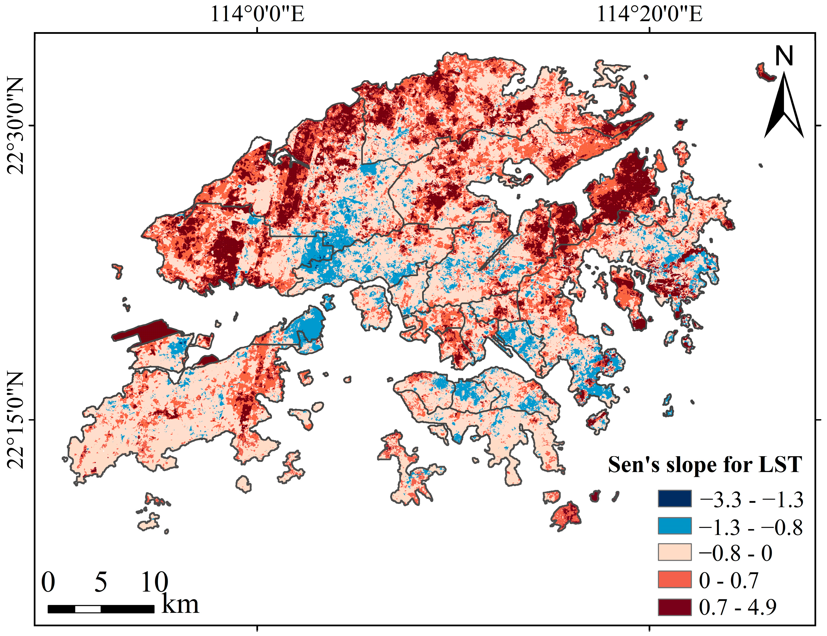
3.3. Sen’s Slope Analysis for Trend Detection

In this study, we integrated Sen’s slope analysis for providing initial insights into the trends of LST and land cover changes over time. Sen’s slope estimator is widely used for estimating the trend slope in a sample of n data pairs using a nonparametric method [56]. It employs a linear model to determine trends, and the variance of the residuals should be constant over time. This trend is calculated as follows:

f(t) = Qt + B

(2)

in which f(t) represents the LST value, Q is the slope trend value, t is the time, and B is a constant. The data pairs are computed using the following equation:

$$Q_i=\frac{x_j-x_i}{j-i}$$

(3)

where $x_j$ is the data value at time j, and $x_i$ is the data value at time i (j > i). The continuous trend of the observation points can be obtained using Equation (4). Next, the N values of $Q_i$ are arranged from the smallest to the largest, and the median of Sen’s slope estimator is calculated as

$$Q=\left\{\begin{array}{cc}{Q}_{\left[(N+1)/2\right]},& \mathit{if}n\mathit{is}\mathit{odd}\\ \frac{Q_{[N/2]}+Q_{\left[\right(N+2)/2]}}{2},& \mathit{if}n\mathit{is}\mathit{even}\end{array}\right.$$

(4)

in which, if there are n of $x_j$ in the time series, $N=n(n-1)/2$, where n is the number of periods, which in this study is n = 6.

Subsequently, the slope trend is calculated. Positive and negative values of Q represent an upward or downward trend in the data. The Mann–Kendall test quantifies the significance of trends in a time series [57]. The formula is:

$$S={\sum }_{i=1}^{n-1}{\sum }_{j=i+1}^{n}sgn(x_j-x_i)$$

(5)

where n is the number of data pairs, and $x_j$ and $x_i$ are the data values in time series $j$ and $i$ (j > i), respectively. The $sgn(x_j-x_i)$ sign function is calculated as follows:

$$sgn(x_j-x_i)=\left\{\begin{array}{cc}+1& if{x}_j-x_i>0\\ 0& if{x}_j-x_i=0\\ -1& if{x}_j-x_i<0\end{array}\right.$$

(6)

The variance is computed as

$$Z_S=\left\{\begin{array}{cc}\frac{S-1}{\sqrt{n(n-1)(2n+5)-{\sum }_{i=1}^p{t}_i\left(t_i-1\right)\left(2t_i+5\right)/18}},& ifS>0\\ 0,& ifS=0\\ \frac{S-1}{\sqrt{n(n-1)(2n+5)-{\sum }_{i=1}^p{t}_i\left(t_i-1\right)\left(2t_i+5\right)/18}},& ifS<0\end{array}\right.$$

(7)

in which n is the amount of data from 2017 to 2022, p is the number of repeated data points in six years, and $t_i$ is the number of data points in the pth group. A positive value $Z_s$ indicates an increasing trend; a negative $Z_s$ indicates a decreasing trend. $Z_{1-\alpha /2}$ can be obtained from the standard normal distribution table at a significance level α. If $\left|Z_s\right|\le Z_{1-\alpha /2}$, the null hypothesis is accepted, and the trend in the time series is not significant. Otherwise, it is significant at this level.

3.4. Bivariate Moran’s I Analysis for Spatial Correlation

The bivariate Moran’s I is used to explore spatial dependency between LST and the spectral indices. It can measure the extent of spatial correlation at a local spatial unit [58]. The spatial correlations between SI and LST are calculated using the following equation:

$$I_{SI,LST}=Z_i^{SI}{\sum }_{j=1}^N{W}_{ij}{Z}_j^{LST}$$

(8)

where $I_{SI,LST}$ is the local bivariate Moran’s I range from −1 to 1, the positive value represents a positive spatial relationship, and the negative value implies a negative spatial correlation between the two variables. N is the number of spatial grids. $Z_i^{SI}$ and $Z_j^{LST}$ refer to the standardized value of each SI for the ith spatial unit and the standardized value of LST for the jth unit (j ≠ i), respectively; $W_{ij}$ is a symmetric weight matrix generated between the ith and jth spatial units.

3.5. Random Forest Regression Model for Feature Importance Assessment

This study applied random forest regression to analyze the relationship between LST and UECs. This nonlinear machine learning algorithm considers continuous and categorical data [59]. This algorithm can reveal the importance of each UEC to the LST. According to the literature, this method is more accurate than others [60,61]. It combines the principles of decision trees and ensemble learning to model complex relationships and effectively manages high-dimensional datasets. This method first builds decision trees, each of which is constructed using a random subset of the training data. The ensemble of decision trees collectively makes predictions by averaging or aggregating the predictions from individual trees, providing a robust, stable estimation of the target variable. During the training phase, the random forest regression algorithm recursively partitions the feature space to create decision trees. Splitting is based on the target variable (i.e., LST) and its associated values (i.e., UECs), which minimize the prediction error. At each split, a subset of the available predictor variables is randomly selected to further enhance the diversity and independence of the trees in the ensemble. This process continues until a predefined stopping criterion is satisfied, such as reaching a specified maximum tree depth or the minimum number of samples required for further splitting [62]. Once trained, the accuracy and performance of the model are evaluated by the coefficient of determination (R²). These metrics assess the ability of the model to capture the relationships between the target and associated variables.

In this study, the analysis was performed using the scikit-learn package in Python. To mitigate the risk of model overfitting, we have taken rigorous steps during model calibration and validation, including cross-validation, hyperparameter tuning, feature selection, and regularization techniques [63]. In this study, we utilized the random forest model to predict LST, combining multiple decision trees into a robust ensemble model. Our dataset was split into an 80% training set and a 20% testing set for robust evaluation. We optimized key hyperparameters using the Optuna library, including the number of trees (n_estimators = 100) and the maximum depth of each tree (max_depth = 5), tailoring the model to the unique complexities of our dataset. To ensure reproducibility in our analysis and maintain consistency, we selected a specific value, 42, for the “random_state” parameter during the train–test split. It is important to note that alternative values can also be utilized for this parameter without affecting the model’s performance.

4. Results

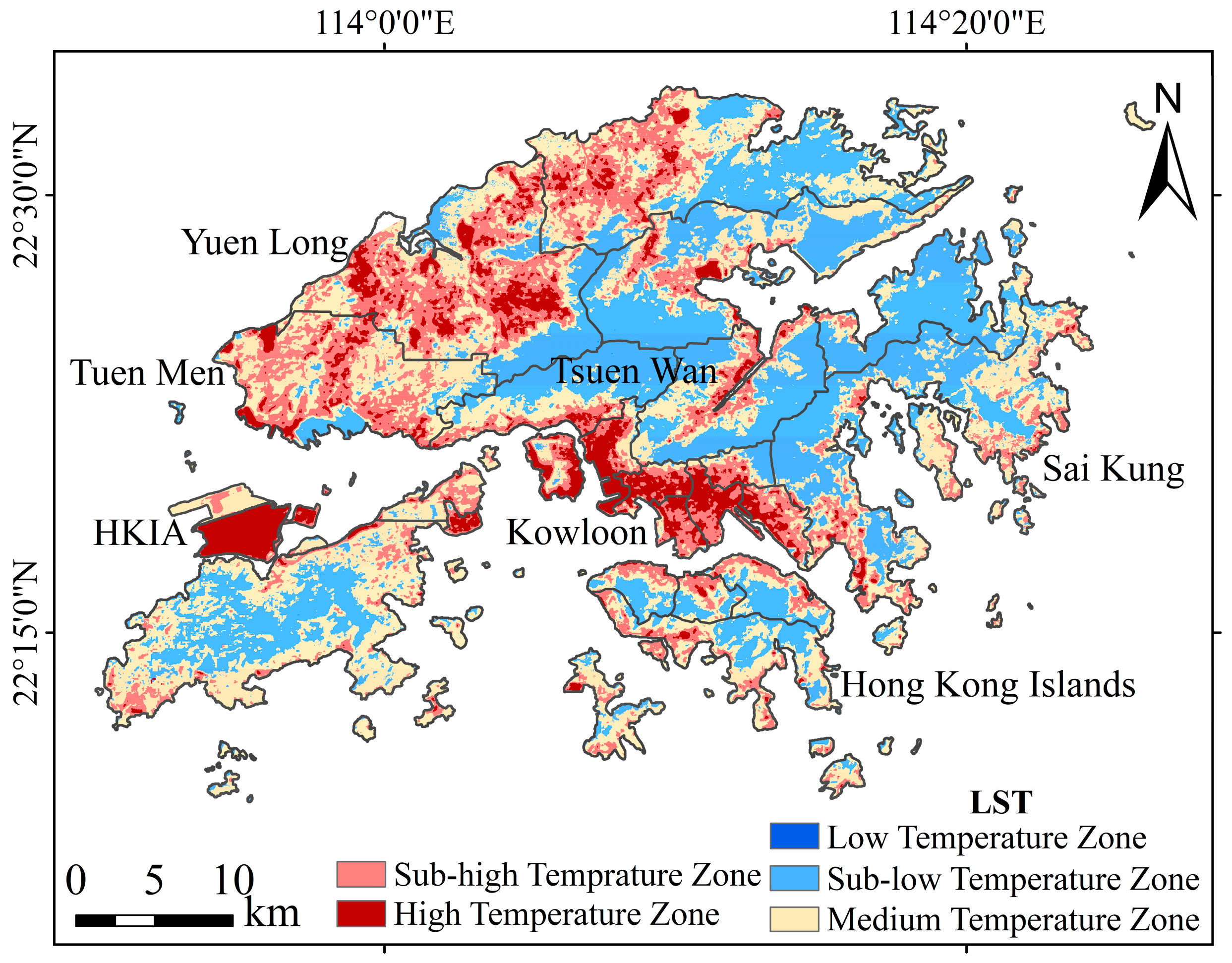
4.1. Spatial and Temporal Patterns of LST

The annual average composite LST from 2017 to 2022 was obtained using GEE. The images used are listed in

Table A1. Specific dates of all satellite images used in our study for each year from 2017 to 2022.

Landsat Scene ID	Date Acquired
LC81210442017001LGN01	1 January 2017
LC81220442017008LGN01	8 January 2017
LC81220452017008LGN01	8 January 2017
LC81210442017049LGN00	18 February 2017
LC81210452017049LGN00	18 February 2017
LC81220442017120LGN00	30 April 2017
LC81220452017120LGN00	30 April 2017
LC81210452017129LGN00	9 May 2017
LC81210452017161LGN00	10 June 2017
LC81210442017209LGN00	28 July 2017
LC81210452017225LGN00	13 August 2017
LC81220442017232LGN00	20 August 2017
LC81220452017232LGN00	20 August 2017
LC81210442017241LGN00	29 August 2017
LC81210452017241LGN00	29 August 2017
LC81210452017289LGN00	16 October 2017
LC81220442017296LGN00	23 October 2017
LC81220452017296LGN00	23 October 2017
LC81210442017305LGN00	1 November 2017
LC81210452017305LGN00	1 November 2017
LC81210442017321LGN00	17 November 2017
LC81210442017337LGN00	3 December 2017
LC81210442017353LGN00	19 December 2017
LC81220442018011LGN00	11 January 2018
LC81220442018043LGN00	12 February 2018
LC81220452018043LGN00	12 February 2018
LC81210442018068LGN00	9 March 2018
LC81220442018091LGN00	1 April 2018
LC81220452018091LGN00	1 April 2018
LC81210452018100LGN00	10 April 2018
LC81220452018123LGN00	3 May 2018
LC81210442018212LGN00	31 July 2018
LC81210452018212LGN00	31 July 2018
LC81210442018276LGN00	3 October 2018
LC81210452018276LGN00	3 October 2018
LC81210442019023LGN00	23 January 2019
LC81210452019023LGN00	23 January 2019
LC81210452019039LGN00	8 February 2019
LC81210442019071LGN00	12 March 2019
LC81220452019078LGN00	19 March 2019
LC81210452019087LGN00	28 March 2019
LC81210452019119LGN00	29 April 2019
LC81220452019158LGN00	7 June 2019
LC81210442019167LGN00	16 June 2019
LC81210442019199LGN00	18 July 2019
LC81220452019206LGN00	25 July 2019
LC81220442019222LGN00	10 August 2019
LC81220452019222LGN00	10 August 2019
LC81220452019254LGN00	11 September 2019
LC81210442019263LGN00	20 September 2019
LC81210452019263LGN00	20 September 2019
LC81220442019270LGN00	27 September 2019
LC81220452019270LGN00	27 September 2019
LC81210452019279LGN00	6 October 2019
LC81210442019295LGN00	22 October 2019
LC81210452019295LGN00	22 October 2019
LC81220442019302LGN00	29 October 2019
LC81210442019311LGN00	7 November 2019
LC81220442019318LGN00	14 November 2019
LC81220452019318LGN00	14 November 2019
LC81210442019327LGN00	23 November 2019
LC81210452019327LGN00	23 November 2019
LC81220442019334LGN00	30 November 2019
LC81220452019334LGN00	30 November 2019
LC81210452019343LGN00	9 December 2019
LC81220452020017LGN00	17 January 2020
LC81220442020049LGN00	18 February 2020
LC81210442020106LGN00	15 April 2020
LC81210452020106LGN00	15 April 2020
LC81210452020138LGN00	17 May 2020
LC81210452020170LGN00	18 June 2020
LC81220452020193LGN00	11 July 2020
LC81220452020209LGN00	27 July 2020
LC81210452020234LGN00	21 August 2020
LC81220442020241LGN00	28 August 2020
LC81220442020321LGN00	16 November 2020
LC81220452020321LGN00	16 November 2020
LC81210442020330LGN00	25 November 2020
LC81220442020337LGN00	2 December 2020
LC81220452020337LGN00	2 December 2020
LC81210442020362LGN00	27 December 2020
LC81210452020362LGN00	27 December 2020
LC81220442021003LGN00	3 January 2021
LC81220452021003LGN00	3 January 2021
LC81210442021012LGN00	12 January 2021
LC81210452021012LGN00	12 January 2021
LC81220442021019LGN00	19 January 2021
LC81210442021028LGN00	28 January 2021
LC81220442021035LGN00	4 February 2021
LC81220452021035LGN00	4 February 2021
LC81220442021051LGN00	20 February 2021
LC81220452021051LGN00	20 February 2021
LC81210452021060LGN00	1 March 2021
LC81210442021076LGN00	17 March 2021
LC81210452021076LGN00	17 March 2021
LC81210442021092LGN00	2 April 2021
LC81210452021092LGN00	2 April 2021
LC81220452021147LGN00	27 May 2021
LC81210452021188LGN00	7 July 2021
LC81220442021195LGN00	14 July 2021
LC81220452021195LGN00	14 July 2021
LC81210442021204LGN00	23 July 2021
LC81210452021204LGN00	23 July 2021
LC81210452021236LGN00	24 August 2021
LC81210442021252LGN00	9 September 2021
LC81210442021268LGN00	25 September 2021
LC81210452021268LGN00	25 September 2021
LC81220442021275LGN00	2 October 2021
LC81220452021275LGN00	2 October 2021
LC81210442021284LGN00	11 October 2021
LC81210452021284LGN00	11 October 2021
LC81210442021316LGN00	12 November 2021
LC81210442021332LGN00	28 November 2021
LC81220442021339LGN00	5 December 2021
LC81220452021339LGN00	5 December 2021
LC81210442021348LGN00	14 December 2021
LC81210442021364LGN00	30 December 2021
LC81220442022006LGN00	6 January 2022
LC81220452022006LGN00	6 January 2022
LC81210452022015LGN00	15 January 2022
LC81210442022063LGN00	4 March 2022
LC81210452022063LGN00	4 March 2022
LC81220442022070LGN00	11 March 2022
LC81220452022070LGN00	11 March 2022
LC81210442022095LGN00	5 April 2022
LC81210452022095LGN00	5 April 2022
LC81210452022111LGN00	21 April 2022
LC81210442022175LGN00	24 June 2022
LC81210452022175LGN00	24 June 2022
LC81210452022191LGN00	10 July 2022
LC81210442022207LGN00	26 July 2022
LC81210452022207LGN00	26 July 2022
LC81220442022214LGN00	2 August 2022
LC81220452022214LGN00	2 August 2022
LC81210442022239LGN00	27 August 2022
LC81210452022239LGN00	27 August 2022
LC81220442022246LGN00	3 September 2022
LC81220452022246LGN00	3 September 2022
LC81210442022255LGN00	12 September 2022
LC81210452022255LGN00	12 September 2022
LC81210442022287LGN00	14 October 2022
LC81210452022287LGN00	14 October 2022
LC81220442022294LGN00	21 October 2022
LC81220452022294LGN00	21 October 2022
LC81210452022319LGN00	15 November 2022
LC81220442022342LGN00	8 December 2022
LC81220452022342LGN00	8 December 2022
LC81220442022358LGN00	24 December 2022
LC81220452022358LGN00	24 December 2022

. The six-year average value was calculated, and the standard deviation was used for classification. The resulting classification is shown in Figure 3.

The results depict the spatial distribution of LST in Hong Kong. LST values were classified into five temperature zones: low temperature (<21 °C), sub-low temperature (21–27 °C), medium temperature (27–30 °C), sub-high temperature (30–33 °C), and high temperature (33–50 °C). Research has identified the high-temperature zone as a UHI [8]. The sub-low-temperature zone covered the largest area of Hong Kong, extending across the central, northern, northeastern, and southern regions. The medium-temperature zone and sub-high-temperature zones exhibited similar coverage. By contrast, the high-temperature and sub-high-temperature zones were concentrated in specific areas, particularly in the south-central region encompassing Kowloon, a part of the area in Tsuen Wan, and the western region, including Yuen Long. Notably, the HKIA was in the high-temperature zone.

The trend degrees presented in this study represent the average rate of change from 2017 to 2022, providing an overview of the overall temporal patterns The temporal trend of LST from 2017 to 2022 was analyzed using the natural breaks Jenks classification method [64,65].

Table 2. Area percentage of different Sen’s slope for LST.

Sen’s Slope for LST	Description	Area Percentage
−3.3 to −1.3	Rapid decrease	0.11%
−1.3 to −0.8	Slow decrease	8.87%
−0.8 to 0	Slight decrease	50.63%
0 to 0.7	Slow increase	25.75%
0.7 to 4.9	Rapid increase	14.63%

presents the LST trends in five degrees: rapid decrease (<−1.3), slow decrease (from −1.3 to −0.8), slight decrease (from −0.8 to 0), slight increase (from 0 to 0.7), and rapid increase (from 0.7 to 4.9). The majority of the regions in Hong Kong exhibited a slight downward trend in LST, indicating a general cooling pattern. As shown in Figure 4, the northeastern and western parts of the city exhibited an extreme upward LST trend, with the Sen’s slope ranging between 0.7 to 4.9, highlighting regions and changes of particular interest. This finally contributed to an overall annual increase in LST values. Notably, the third runway area at HKIA, located in the western region, exhibited a prominent rapid increase in LST, reaching a maximum value of 4.7.

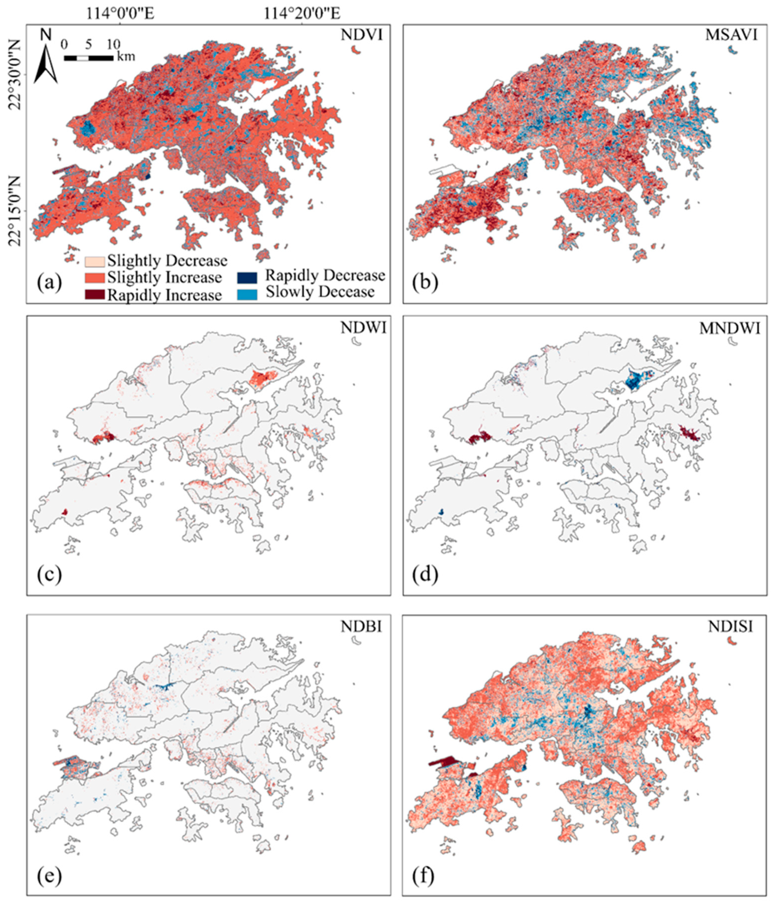
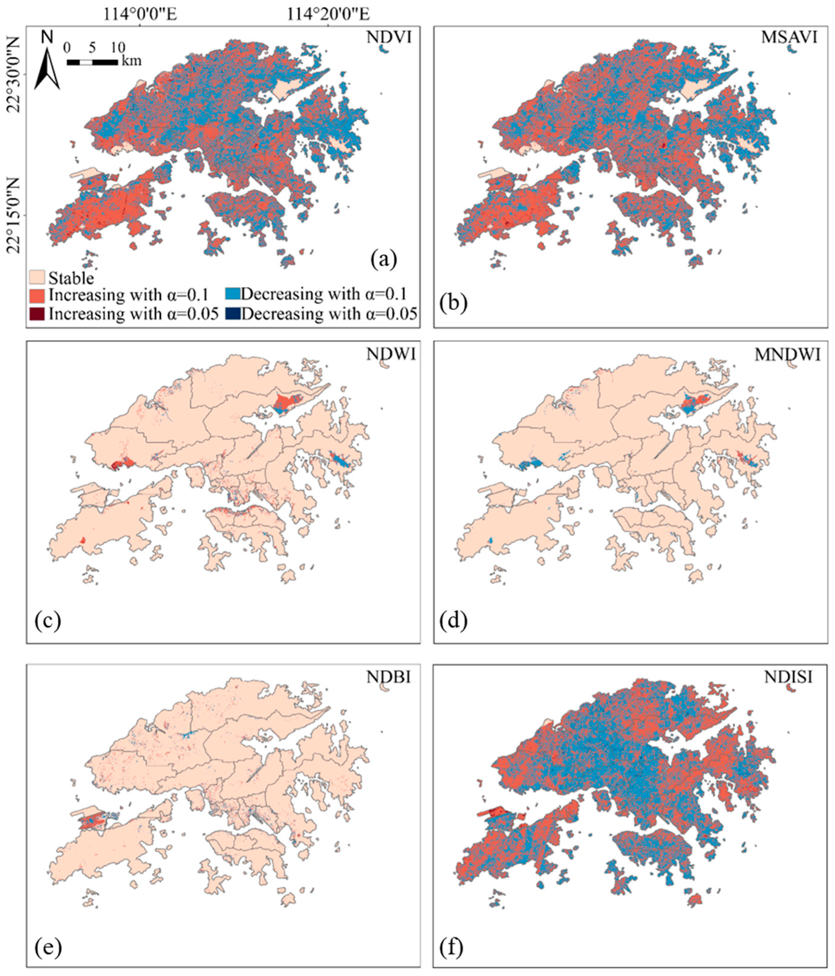
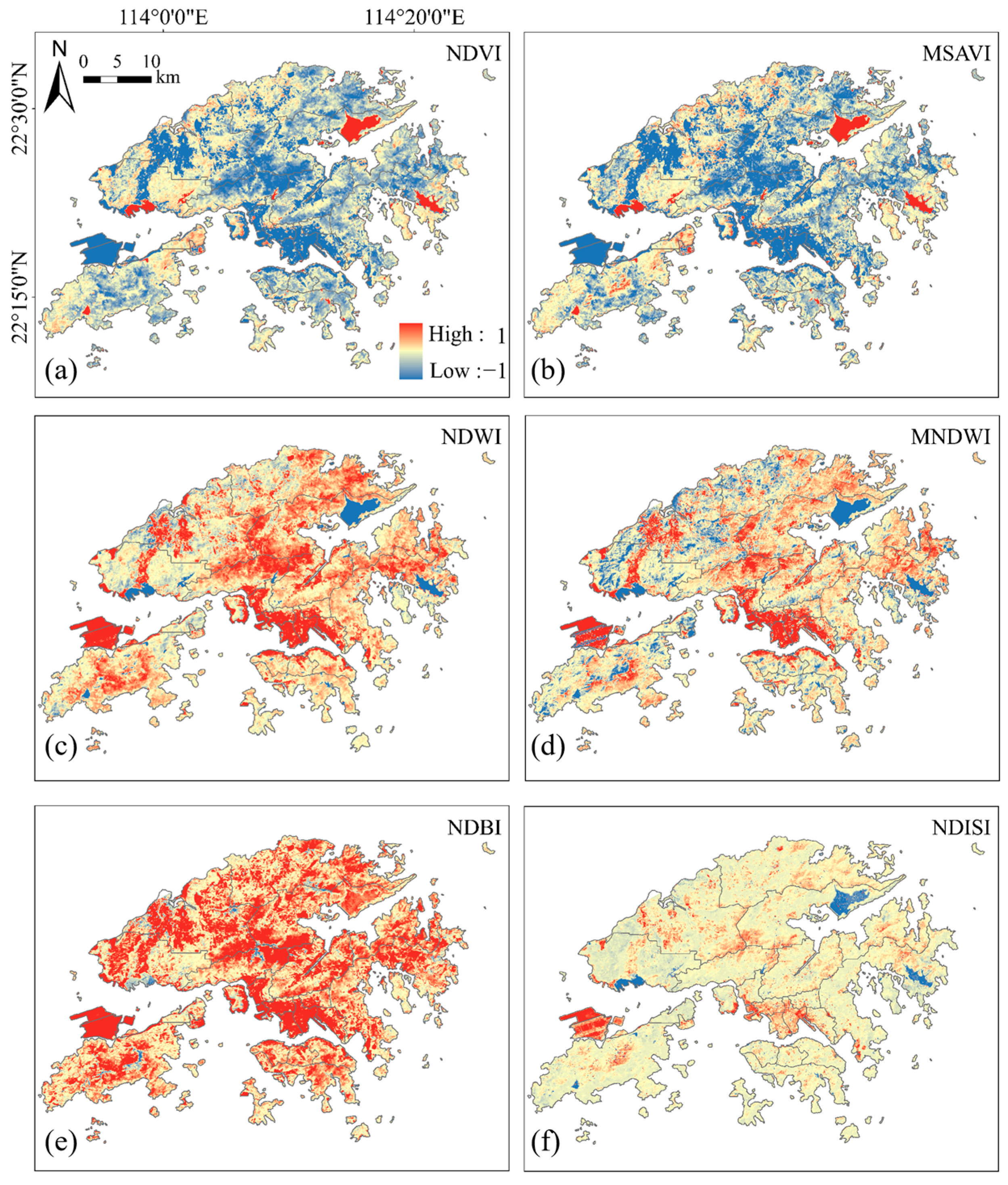
4.2. Spatial and Temporal Patterns of UECs

As aforementioned, analyzing the influence of UECs includes the assessment of spectral indices and land use types. The procedure of the spatiotemporal pattern analysis of the spectral indices was the same as that for the LST analysis. Figure 5 presents the spatial distribution of vegetation, water, and built-up indices. Figure 5a,b present the variations in vegetation indices across the study area in five classes: bare area, low vegetation, medium vegetation, sub-high vegetation, and high vegetation (

Table 3. Category value ranges for NDVI and MSAVI.

Category	NDVI	MSAVI
Bare land	−0.1–0.2	−0.1–0.2
Low vegetation	0.2–0.4	0.2–0.4
Medium vegetation	0.4–0.6	0.4–0.6
Sub-high vegetation	0.6–0.8	0.6–0.8
High vegetation	0.8–1.0	0.8–1.0

). The spatial distributions of the NDVI and MSAVI exhibited a high degree of similarity, with high vegetation cover areas concentrated in the central and southern regions, namely, the New Territories and Hong Kong Island. Conversely, areas with low vegetation cover were observed in the eastern part of HKIA and the Kowloon region in the central-southern part of the study area.

Regarding the water indices, Figure 5c,d depict the division into water bodies and others. The water bodies were primarily distributed in the western and northwestern regions, represented by the High Island Reservoir and Plover Cove Reservoir. Figure 5e,f present the built-up indices in four classes: other, low built-up, medium built-up, and high built-up. Notably, the spatial distribution of the built-up indices contrasted with that of the NDVI, with high-value areas predominantly situated in the central-southern part of the study area, encompassing Kowloon, Hong Kong Island near Victoria Harbor, and HKIA (on the left side of the figure).

To further explore the trends of the spectral indices during 2017–2022, this study applied Sen’s slope analysis (Figure 6). Figure 6 shows the trend results of the spectral indices from 2017 to 2022. The first row shows the variation in vegetation indices. Overall, vegetation cover had an upward trend in most areas. Figure 6c,d show the trends of the water body indices, where most of the gray areas are neither water bodies nor change areas, consistent with Figure 5c,d. Notably, in Figure 6e, the NDBI of HKIA in the west substantially changed, and the rest of the region remained approximately the same.

The Mann–Kendall significance test result in Figure 7 is corresponding with the change trend, α = 0.05 represents 1.96 ≤ |Z| < 2.58, which refers to significant change. A = 0.01 means 1.645 ≤ |Z| << 1.96, which refers to a slight significant change. This result can be used to aid in interpreting the spectral indices changes in Figure 6.

The pattern of land use types was divided into 20 classes; the results are shown in Figure 8. The results illustrate the land use types in 2018 and 2020. Generally, the vegetation area accounted for a large percentage of Hong Kong, almost 71.11% in 2018 and 72.30% in 2020. The construction area accounted for 20.92% and 19.30% of the total area in 2018 and 2020, respectively. Vegetation cover had a slight upward trend, and the built-up area had a slight downward trend. The land use distributions in Figure 8a,b were essentially unchanged. The most notable event during these two years was the construction of the third runway at the HKIA in the southwest corner of Hong Kong, and the airport is expanding.

The impact of land use change on LST was explored in this study. The results suggest that such an influence varied among land use types and their changes (

Table 4. LST change in top five areas of land use and land use change.

Land Use/Land Use Change	LST Change/°C	Area/km2
Forest	−1.643	454.8
Urban	−1.033	205.0
Woodland	−0.826	175.2
High coverage grass	−1.271	261.3
Reservoir pond	0.173	72.6
Urban- > Other construction	−0.979	15.0
Forest- > High coverage grass	−1.159	8.3
High coverage grass- > Forest	−1.178	7.1
Rural land- > Forest	−2.477	6.9
Urban- > Forest	−1.137	4.3

and Figure A1).

Table 4 provides insights into the influence of the top five land use categories and the top five land use changes on LST. For example, Forests covered the most extensive area among all land use types, approximately 454.8 km². Land use change from urban areas to other construction areas had the highest number of changes, encompassing 15.0 km² between 2018 and 2020.

The top four land use types were associated with vegetation, and their impact on LST change was predominantly negative. This phenomenon suggests that areas characterized by these land use types contribute to the decreased surface temperature. Conversely, the presence of reservoir ponds positively influenced LST change, with an average temperature increase of 0.173 °C observed over an area of 72.6 km². Regarding land use type changes, the transition from rural land to forest had the most substantial change: a decrease of −2.477 °C. This change covered an area of 6.9 km², ranking fourth among the land use change types. This finding supports the hypothesis that converting land use types from built-up areas to vegetated areas significantly affects surface temperature variability. The results in Table 4 emphasize the importance of considering land use categories and changes to understand the patterns and dynamics of LST.

4.3. Correlation Analysis between LST and UECs

An annual LST and spectral index change graph was drafted to further explore the relationship between LST and UECs (Figure 9). First, we generated average values for each variable spanning six years. Then, we conducted a local bivariate Moran’s I analysis and the results illustrated the spatial associations between LST and the spectral indices in our study area.

Figure 9 depicts the annual average temporal trends of LST and spectral indices. LST gradually increased from 2017 to 2022, with a minimum value of 21.13 °C in 2018 and a maximum value of 23.46 °C in 2022. The trend exhibited a “V” from 2017 to 2019 and an inverted “V” from 2018 to 2020. Figure 9a presents a similar pattern between the vegetation indices (NDVI and MSAVI), with the lowest values in 2019 and a “V”-shaped trend between 2018 and 2020. Figure 9b presents a similar trend for the water indices, with peaks in 2020. Figure 9c presents distinct behavior for the built-up indices (NDBI and NDISI), with significant changes in the NDBI.

Next, the specific relationship was calculated using the Pearson correlation method to analyze the connection (Figure 10). The heat map results include LST and the spectral indices, with the coefficient ranging from −0.96 to 1. Positive values indicate a positive correlation; negative values indicate a negative correlation. A larger absolute value indicated a stronger correlation. A summary of the results is as follows: (1) The first row showed the correlation coefficient with the LST. Moreover, LST had a negative correlation with vegetation and water indices and a positive correlation with built-up indices. (2) The highest positive value was between the LST and NDBI (0.74), and the lowest negative value (−0.96) was between the LST and NDWI. This result suggests that the relationship between LST and NDWI/NDBI is strong, indicating that changes in NDWI/NDBI result in corresponding changes in LST. (3) The heatmap also demonstrates the relationship between the spectral indices. For example, the NDVI was positively correlated with the MSAVI (0.95) and negatively correlated with the NDWI and NDBI. This result supports those in the literature [50,66].

To capture the relationship in spatial distribution, we used the local bivariate Moran’s I to analyze the cross-correlation between LST and the spectral indices (Figure 11). The average value was first generated for each variable in the six years before conducted local bivariate Moran’s I and the results demonstrated the spatial association between LST and the spectral indices in space. The positive correlation between the LST and vegetation indices was concentrated in the western part of Hong Kong, namely, the Tuen Mun and island districts (Figure 11a,b). In addition, the correlation results of the NDBI and NDISI contrasted with those of the NDVI and MSAVI. The positive correlation was mainly in HKIA and the coast of Victoria Harbor, which includes the Tsim Sha Tsui district and Hong Kong Island.

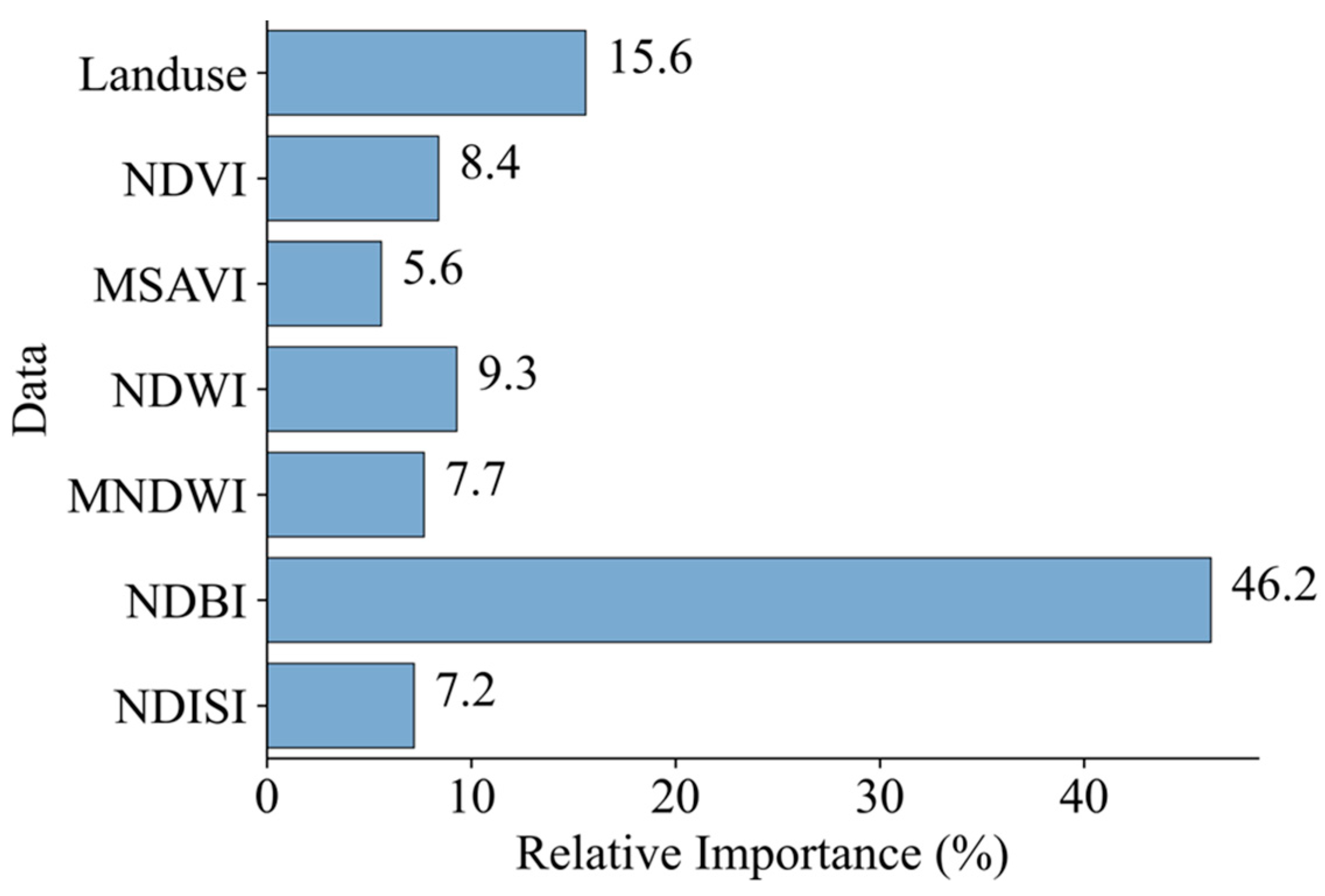
4.4. Random Forest Analysis of Feature Importance

The results of the random forest regression model revealed the relative importance of each UEC in the spatial pattern of the LST (Figure 12).

Figure 12 presents the importance values of each UEC for LST. These importance values reflect the contribution of UECs to the variation in LST. The R² of this model is 0.74. In particular, NDBI had the highest importance value: 46.2%. The substantial importance of the NDBI suggests that urbanization and the associated increase in built-up areas contribute significantly to increasing the LST. By contrast, the NDVI and MSAVI exhibited lower importance values than NDBI, with 8.4% and 5.6%, respectively. These indices capture the presence and health of the vegetation cover. Their relatively low importance values suggest that vegetation cover moderately influences LST variations more than built-up areas. The NDWI and MNDWI had importance values of 9.3% and 7.7%, respectively. These indices represent the presence of water bodies that can act as coolants and reduce the LST. The comparable importance values of the NDWI and MNDWI indicate that both indices contribute similarly to explaining LST variations. The importance value of the NDISI was 7.2%. This index characterizes impervious surfaces, such as concrete or asphalt, which absorb and retain heat, contributing to increasing the LST. Although the importance value of the NDISI is lower than those of the NDBI, NDWI, and MNDWI, NDISI plays a significant role in explaining LST variations. Finally, land use, represented by an importance value of 15.6%, captured the effects of different land use types on LST and thermal properties. Although its importance value is relatively lower than that of the NDBI, it still indicates the relevance of land use in influencing LST patterns.

In summary, the importance values assigned to each spectral index highlighted the varying contributions of built-up areas (53.4%), water bodies (17%), vegetation cover (14%), and land use (15.6%) to LST variations. The high importance values of the NDBI suggest that built-up areas have the most substantial impact on LST, followed by water bodies and land use. Although influential, vegetation cover exhibited a relatively moderate influence compared with other factors. Understanding these differences can inform strategies for urban planning and heat island mitigation.

5. Discussion

5.1. Further Analysis of HKIA

One objective of this study was to investigate the mechanisms that affect the variation in LST. To achieve this objective, we narrowed the focus to the local area of Hong Kong, specifically HKIA. Using HKIA as the research object provided a comprehensive understanding of how urbanization influences LST and contributes to the UHI effect.

As shown in Figure 13a, the LST of the airport’s third runway in the northwest direction significantly increased from 2017 to 2022. This observation is supported by the trends shown in Figure 13b–d, which demonstrate the corresponding changes in spectral indices for the third runway area. Specifically, the NDVI in Figure 13b exhibits a decreasing trend for the third runway and airport, indicating a decline in vegetation cover. Similarly, Figure 13c displays a rapid decrease in the NDWI, suggesting a reduction in the number of water bodies in the area. By contrast, Figure 13d exhibits a notable upward trend in the NDBI, indicating increased building cover.

These relationships support the suggestion that the increase in LST is primarily due to the process of reclamation [67]. HKIA, including parts of the main airport, an artificial island, and a third runway, was constructed through land reclamation. This process leads to a reduction in water bodies and the expansion of built-up areas. Water bodies have a cooling effect, negatively correlated with LST, and built-up areas exhibit a positive correlation, increasing the LST. The combined effect of decreasing water bodies and increasing built-up areas contributed to the UHI effect at the airport. The optical images in Figure 13e,f provide evidence to support this observation. Furthermore, a portion of the third runway had rapid growth in vegetation cover, possibly for improved runway identification purposes [68]. Although these vegetation patches mitigated the UHI effect, they did not halt the upward trend. Similar findings have been reported in other reclaimed areas, such as Bahrain International Airport and Istanbul Airport [69,70].

We considered the findings on the impact of the reclamation on LST at HKIA and posed the following recommendations to inform future reclamation projects: First, comprehensive environmental impact assessments should be conducted before engaging in reclamation activities, particularly to assess the potential consequences for water bodies and built-up areas. These assessments should consider the potential loss of natural habitats and associated implications for temperature regulation. Second, adopting innovative urban planning strategies would optimize the spatial layout of airports and their surrounding areas, reducing the negative impacts of reclamation on LST. These strategies involve optimizing the distribution of built-up areas, preserving or restoring water bodies, and incorporating natural cooling elements, such as water features or greenspaces, to counterbalance the heat generated by airport infrastructure.

5.2. Implications for Urban Planning and Management

This study focused on the influence of UECs on LST in Hong Kong. The results imply that differentiated and targeted planning strategies based on the effects of UECs on LST can be developed to reduce LST effectively. Additionally, by considering the relationship between LST and spectral indices, along with increasing the percentage of vegetation cover or decreasing the proportion of building areas in urban environment, effective control of reclamation may be the most meaningful approach for reducing LST in regions with high population density, such as Hong Kong.

Because of the significant prevalence of the UHI effect in Hong Kong, particularly in densely built-up areas, prioritizing interventions in these high-temperature zones is crucial. Construction areas within the urban fabric exhibit elevated temperatures, making them focal points for targeted attention. Integrating green spaces with vegetation should be the central focus of urban planning initiatives. This decision would help mitigate the UHI effect by providing shade, transpiration, and evapotranspiration, cooling the surrounding environment. Moreover, the preservation and protection of water bodies should be emphasized to leverage their moderating influence on temperature.

Furthermore, integrating sustainable development principles with infrastructure construction in urban areas is imperative. The implementation of concepts such as green roofs and permeable surfaces can effectively mitigate the UHI effect and enhance urban resilience. These measures facilitate the integration of nature-based solutions and sustainable practices into built environments.

As part of our recommendation to the government, UHI mitigation strategies should be enhanced by incorporating the following key elements: prioritizing interventions in high-temperature zones, integrating green spaces and vegetation, emphasizing the preservation of water bodies, and incorporating sustainable development principles into the infrastructure of built-up areas.

5.3. Limitations and Recommendations for Further Research

This study had limitations that warrant consideration. First, the data resolution and quality used in the analysis would be improved in further research by incorporating data with higher spatiotemporal resolution than the data we used. Such data would provide more detailed and accurate information than we provided, deepening the understanding of the relationship between LST and the spectral indices. Additionally, one limitation of our study is the relatively short six-year time series dataset, which may limit the robustness of trend analysis results. Additionally, this timeframe may not fully capture long-term trends or account for natural variability. Consequently, the interpretation of trends should be made cautiously, recognizing the potential for variability due to the limited temporal scope. Therefore, we recommend that future research endeavors to consider encompassing a more extensive temporal perspective, which could provide valuable insights into the evolution of LST in urban areas [71,72,73].

Additionally, this study did not consider the influence of social and economic factors resulting from human activities and the increasing population on LST. Thus, further research should integrate socioeconomic data to gain insights into the contextual factors shaping temperature patterns, deepening the holistic understanding of the complex interactions among LST, spectral indices, and socioeconomic variables. While this study uses high LST as a proxy for UHI, it is essential to note the inherent uncertainties this may introduce, such as the influence of varied urban land covers, fluctuations in daily temperature patterns, and atmospheric disturbances. Future research could consider employing more rigorous methods to identify UHI regions accurately. It is worth noting that another potential limitation of our study lies in the choice of the model. While we have employed the random forest model effectively to explore relationships within the available data, the limited temporal scope may constrain its ability to capture long-term trends and natural variability. Future research may benefit from comparing various machine learning models to provide a more comprehensive assessment of performance and applicability.

6. Conclusions

This study investigated the influence of UECs on LST in Hong Kong. The primary objective was to deepen the understanding of the factors and mechanisms contributing to the spatial and temporal variations in LST in urban areas characterized by significant development. The implications of these findings are crucial for effectively regulating LST and promoting sustainable urban development. The key conclusions derived from the analysis are summarized as follows:

(1)

Spatial and temporal LST patterns: The analysis revealed spatial variations in LST across different locations in Hong Kong. The UHI effect was observed in areas such as Tsim Sha Tsui and Hong Kong Island, particularly along Victoria Harbor. Notably, HKIA also exhibited high temperatures and experienced a rapid increase in LST from 2019 to 2022. The UEC analysis indicated slight changes in water bodies and built-up areas, whereas the extent of vegetation remained relatively stable.

(2)

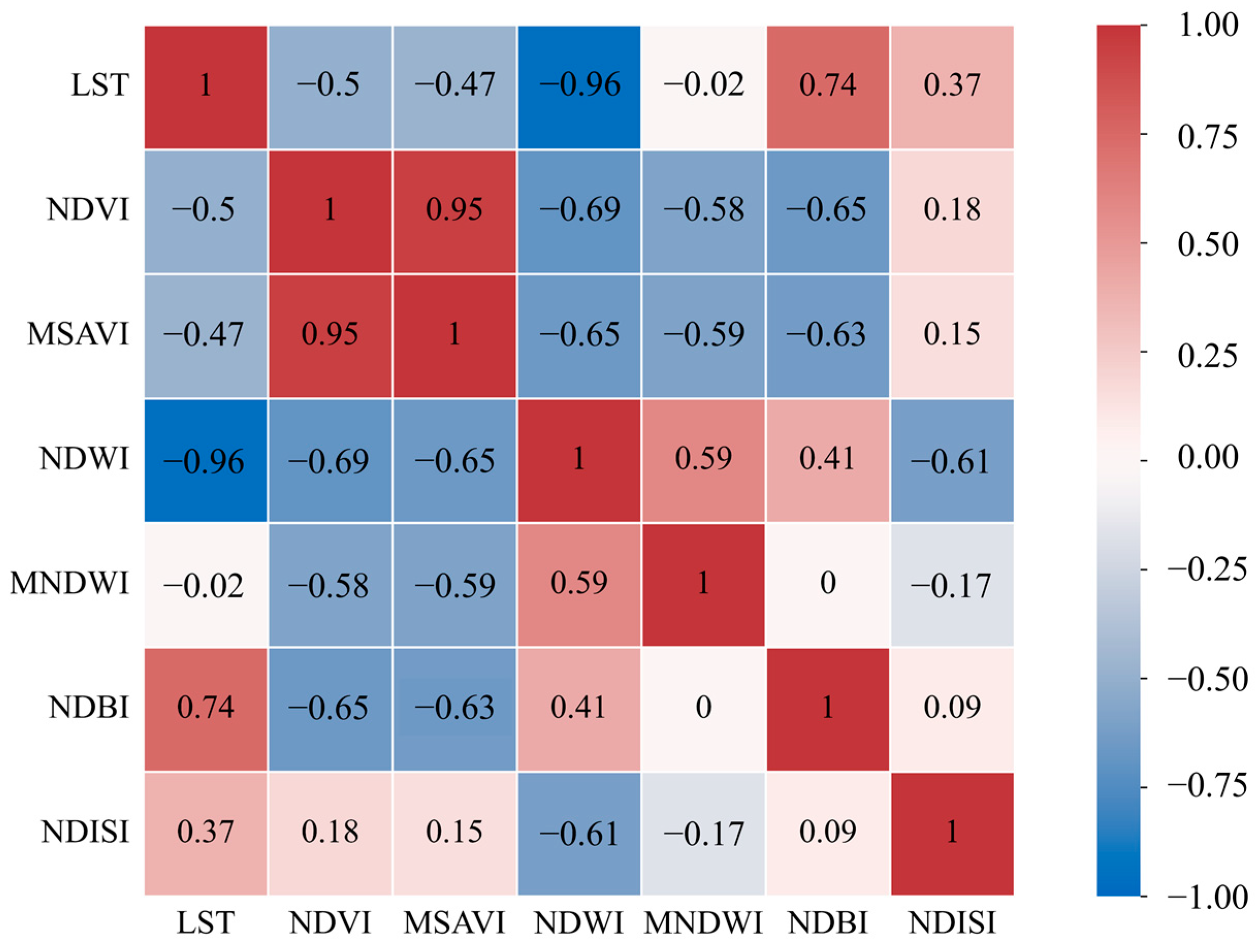
Relationship between LST and UECs: We examined the relationship between LST and UECs through spatial correlation analysis utilizing Pearson’s correlation and the local bivariate Moran’s I. Our analysis revealed significant correlations between LST and UECs. Specifically, vegetation cover and water bodies exhibited negative correlations with LST, with Pearson’s correlation coefficients both of −0.49, indicating a cooling effect. Conversely, there was a positive correlation between LST and built-up areas, with a Pearson’s correlation coefficient of 0.56, suggesting a contribution to higher temperatures. These findings emphasize the importance to consider the impact of land use type on LST when monitoring and managing urban environments.

(3)

Feature importance of UECs to LST: A relative importance analysis using the random forest method highlighted the contribution of UECs to LST. Among the factors examined, built-up areas emerged as the most influential, accounting for approximately 53.4% of LST variation. Additionally, this study emphasized the significance of considering the impact of reclamation on LST, particularly in the context of HKIA.

These findings provide valuable insights into the complex relationship between UECs and LST in highly urbanized areas, such as Hong Kong. Specifically, our research reveals that certain UECs significantly affected LST patterns. These insights improve the understanding of the factors influencing LST and provide guidance for regulating and managing urban environments for sustainable development, such as implementing urban design strategies that mitigate the UHI effect.

References

1. Cohen, B. Urbanization in Developing Countries: Current Trends, Future Projections, and Key Challenges for Sustainability. Technol. Soc. 2006, 28, 63–80. [Google Scholar] [CrossRef]
2. Mcdonald, R.I.; Kareiva, P.; Forman, R.T.T. The Implications of Current and Future Urbanization for Global Protected Areas and Biodiversity Conservation. Biol. Conserv. 2008, 141, 1695–1703. [Google Scholar] [CrossRef]
3. Srikanth, K.; Swain, D. Urbanization and Land Surface Temperature Changes over Hyderabad, a Semi-Arid Mega City in India. Remote Sens. Appl. Soc. Environ. 2022, 28, 100858. [Google Scholar] [CrossRef]
4. Landsberg, H.E. The Urban Climate; Academic Press: Cambridge, MA, USA, 1981; ISBN 978-0-08-092419-9. [Google Scholar]
5. Grimm, N.B.; Faeth, S.H.; Golubiewski, N.E.; Redman, C.L.; Wu, J.; Bai, X.; Briggs, J.M. Global Change and the Ecology of Cities. Science 2008, 319, 756–760. [Google Scholar] [CrossRef]
6. Howard, L. The Climate of London: Deduced from Meteorological Observations Made in the Metropolis and at Various Places Around It; Harvey, Darton, J., Longman, A.A., Highley, H.S., Hunter, R., Eds.; Harvey and Darton: London, UK, 1833. [Google Scholar]
7. Tomlinson, C.J.; Chapman, L.; Thornes, J.E.; Baker, C.J. Including the Urban Heat Island in Spatial Heat Health Risk Assessment Strategies: A Case Study for Birmingham, UK. Int. J. Health Geogr. 2011, 10, 42. [Google Scholar] [CrossRef] [PubMed]
8. Li, G.; Zhang, X.; Mirzaei, P.A.; Zhang, J.; Zhao, Z. Urban Heat Island Effect of a Typical Valley City in China: Responds to the Global Warming and Rapid Urbanization. Sustain. Cities Soc. 2018, 38, 736–745. [Google Scholar] [CrossRef]
9. Sun, Y.; Hu, T.; Zhang, X.; Li, C.; Lu, C.; Ren, G.; Jiang, Z. Contribution of Global Warming and Urbanization to Changes in Temperature Extremes in Eastern China. Geophys. Res. Lett. 2019, 46, 11426–11434. [Google Scholar] [CrossRef]
10. Moazzam, M.F.U.; Doh, Y.H.; Lee, B.G. Impact of Urbanization on Land Surface Temperature and Surface Urban Heat Island Using Optical Remote Sensing Data: A Case Study of Jeju Island, Republic of Korea. Build. Environ. 2022, 222, 109368. [Google Scholar] [CrossRef]
11. Singh, P.; Kikon, N.; Verma, P. Impact of Land Use Change and Urbanization on Urban Heat Island in Lucknow City, Central India. A Remote Sensing Based Estimate. Sustain. Cities Soc. 2017, 32, 100–114. [Google Scholar] [CrossRef]
12. Guha, S.; Govil, H.; Diwan, P. Analytical Study of Seasonal Variability in Land Surface Temperature with Normalized Difference Vegetation Index, Normalized Difference Water Index, Normalized Difference Built-up Index, and Normalized Multiband Drought Index. J. Appl. Remote Sens. 2019, 13, 024518. [Google Scholar] [CrossRef]
13. Maheng, D.; Pathirana, A.; Zevenbergen, C. A Preliminary Study on the Impact of Landscape Pattern Changes Due to Urbanization: Case Study of Jakarta, Indonesia. Land 2021, 10, 218. [Google Scholar] [CrossRef]
14. Vautard, R.; Beekmann, M.; Desplat, J.; Hodzic, A.; Morel, S. Air Quality in Europe during the Summer of 2003 as a Prototype of Air Quality in a Warmer Climate. Comptes Rendus Geosci. 2007, 339, 747–763. [Google Scholar] [CrossRef]
15. Founda, D.; Katavoutas, G.; Pierros, F.; Mihalopoulos, N. The Extreme Heat Wave of Summer 2021 in Athens (Greece): Cumulative Heat and Exposure to Heat Stress. Sustainability 2022, 14, 7766. [Google Scholar] [CrossRef]
16. Rango, A.; Laliberte, A.; Herrick, J.E.; Winters, C.; Havstad, K.; Steele, C.; Browning, D. Unmanned Aerial Vehicle-Based Remote Sensing for Rangeland Assessment, Monitoring, and Management. J. Appl. Remote Sens. 2009, 3, 033542. [Google Scholar] [CrossRef]
17. Amiri, R.; Weng, Q.; Alimohammadi, A.; Alavipanah, S.K. Spatial–Temporal Dynamics of Land Surface Temperature in Relation to Fractional Vegetation Cover and Land Use/Cover in the Tabriz Urban Area, Iran. Remote Sens. Environ. 2009, 113, 2606–2617. [Google Scholar] [CrossRef]
18. Kachar, H.; Vafsian, A.R.; Modiri, M.; Enayati, H.; Safdari Nezhad, A.R. Evaluation of spatial and temporal distribution changes of lst using landsat images (case study:Tehran). Int. Arch. Photogramm. Remote Sens. Spat. Inf. Sci. 2015, XL-1-W5, 351–356. [Google Scholar] [CrossRef]
19. Taloor, A.K.; Manhas, D.S.; Kothyari, G.C. Retrieval of Land Surface Temperature, Normalized Difference Moisture Index, Normalized Difference Water Index of the Ravi Basin Using Landsat Data. Appl. Comput. Geosci. 2021, 9, 100051. [Google Scholar] [CrossRef]
20. Zhou, L.; Yuan, B.; Hu, F.; Wei, C.; Dang, X.; Sun, D. Understanding the Effects of 2D/3D Urban Morphology on Land Surface Temperature Based on Local Climate Zones. Build. Environ. 2022, 208, 108578. [Google Scholar] [CrossRef]
21. Yin, S.; Liu, J.; Han, Z. Relationship between Urban Morphology and Land Surface Temperature—A Case Study of Nanjing City. PLoS ONE 2022, 17, e0260205. [Google Scholar] [CrossRef]
22. Guo, G.; Zhou, X.; Wu, Z.; Xiao, R.; Chen, Y. Characterizing the Impact of Urban Morphology Heterogeneity on Land Surface Temperature in Guangzhou, China. Environ. Model. Softw. 2016, 84, 427–439. [Google Scholar] [CrossRef]
23. Zha, Y.; Gao, J.; Ni, S. Use of Normalized Difference Built-up Index in Automatically Mapping Urban Areas from TM Imagery. Int. J. Remote Sens. 2003, 24, 583–594. [Google Scholar] [CrossRef]
24. Yuan, F.; Bauer, M.E. Comparison of Impervious Surface Area and Normalized Difference Vegetation Index as Indicators of Surface Urban Heat Island Effects in Landsat Imagery. Remote Sens. Environ. 2007, 106, 375–386. [Google Scholar] [CrossRef]
25. Dai, F.C.; Lee, C.F.; Zhang, X.H. GIS-Based Geo-Environmental Evaluation for Urban Land-Use Planning: A Case Study. Eng. Geol. 2001, 61, 257–271. [Google Scholar] [CrossRef]
26. Sahoo, S.; Majumder, A.; Swain, S.; Gareema; Pateriya, B.; Al-Ansari, N. Analysis of Decadal Land Use Changes and Its Impacts on Urban Heat Island (UHI) Using Remote Sensing-Based Approach: A Smart City Perspective. Sustainability 2022, 14, 11892. [Google Scholar] [CrossRef]
27. Price, J.C. Using Spatial Context in Satellite Data to Infer Regional Scale Evapotranspiration. IEEE Trans. Geosci. Remote Sens. 1990, 28, 940–948. [Google Scholar] [CrossRef]
28. Sun, D.; Kafatos, M. Note on the NDVI-LST Relationship and the Use of Temperature-Related Drought Indices over North America. Geophys. Res. Lett. 2007, 34, L24406. [Google Scholar] [CrossRef]
29. Liu, L.; Zhang, Y. Urban Heat Island Analysis Using the Landsat TM Data and ASTER Data: A Case Study in Hong Kong. Remote Sens. 2011, 3, 1535–1552. [Google Scholar] [CrossRef]
30. Guha, S.; Govil, H.; Dey, A.; Gill, N. Analytical Study of Land Surface Temperature with NDVI and NDBI Using Landsat 8 OLI and TIRS Data in Florence and Naples City, Italy. Eur. J. Remote Sens. 2018, 51, 667–678. [Google Scholar] [CrossRef]
31. Akher, S.K.; Chattopadhyay, S. Impact of Urbanization on Land Surface Temperature-a Case Study of Kolkata New Town. Int. J. Eng. Sci. IJES 2017, 6, 71–81. [Google Scholar] [CrossRef]
32. Shahfahad; Kumari, B.; Tayyab, M.; Ahmed, I.A.; Baig, M.R.I.; Khan, M.F.; Rahman, A. Longitudinal Study of Land Surface Temperature (LST) Using Mono- and Split-Window Algorithms and Its Relationship with NDVI and NDBI over Selected Metro Cities of India. Arab. J. Geosci. 2020, 13, 1040. [Google Scholar] [CrossRef]
33. Sun, Q.; Wu, Z.; Tan, J. The Relationship between Land Surface Temperature and Land Use/Land Cover in Guangzhou, China. Environ. Earth Sci. 2012, 65, 1687–1694. [Google Scholar] [CrossRef]
34. Forman, R.T.T. Land Mosaics: The Ecology of Landscapes and Regions; Cambridge University Press: Cambridge, UK, 1995; ISBN 978-0-521-47980-6. [Google Scholar]
35. Estoque, R.C.; Murayama, Y.; Myint, S.W. Effects of Landscape Composition and Pattern on Land Surface Temperature: An Urban Heat Island Study in the Megacities of Southeast Asia. Sci. Total Environ. 2017, 577, 349–359. [Google Scholar] [CrossRef] [PubMed]
36. Siqi, J.; Yuhong, W. Effects of Land Use and Land Cover Pattern on Urban Temperature Variations: A Case Study in Hong Kong. Urban Clim. 2020, 34, 100693. [Google Scholar] [CrossRef]
37. Alcantara, C.A.; Escoto, J.D.; Blanco, A.C.; Baloloy, A.B.; Santos, J.A.; Sta. Ana, R.R. Geospatial assessment and modeling of urban heat islands in quezon city, philippines using ols and geographically weighted regression. Int. Arch. Photogramm. Remote Sens. Spat. Inf. Sci. 2019, XLII-4-W16, 85–92. [Google Scholar] [CrossRef]
38. Guo, G.; Wu, Z.; Xiao, R.; Chen, Y.; Liu, X.; Zhang, X. Impacts of Urban Biophysical Composition on Land Surface Temperature in Urban Heat Island Clusters. Landsc. Urban Plan. 2015, 135, 1–10. [Google Scholar] [CrossRef]
39. Lee, S.-I. Developing a Bivariate Spatial Association Measure: An Integration of Pearson’s r and Moran’s I. J. Geogr. Syst. 2001, 3, 369–385. [Google Scholar] [CrossRef]
40. Huang, Z.; Yin, G.; Peng, X.; Zhou, X.; Dong, Q. Quantifying the Environmental Characteristics Influencing the Attractiveness of Commercial Agglomerations with Big Geo-Data. Environ. Plan. B Urban Anal. City Sci. 2023, 23998083231158370. [Google Scholar] [CrossRef]
41. Fan, C.; Myint, S.W.; Zheng, B. Measuring the Spatial Arrangement of Urban Vegetation and Its Impacts on Seasonal Surface Temperatures. Prog. Phys. Geogr. Earth Environ. 2015, 39, 199–219. [Google Scholar] [CrossRef]
42. Kashki, A.; Karami, M.; Zandi, R.; Roki, Z. Evaluation of the Effect of Geographical Parameters on the Formation of the Land Surface Temperature by Applying OLS and GWR, A Case Study Shiraz City, Iran. Urban Clim. 2021, 37, 100832. [Google Scholar] [CrossRef]
43. Grimm, R.; Behrens, T.; Märker, M.; Elsenbeer, H. Soil Organic Carbon Concentrations and Stocks on Barro Colorado Island—Digital Soil Mapping Using Random Forests Analysis. Geoderma 2008, 146, 102–113. [Google Scholar] [CrossRef]
44. Guio Blanco, C.M.; Brito Gomez, V.M.; Crespo, P.; Ließ, M. Spatial Prediction of Soil Water Retention in a Páramo Landscape: Methodological Insight into Machine Learning Using Random Forest. Geoderma 2018, 316, 100–114. [Google Scholar] [CrossRef]
45. Matcham, E.G.; Subburayalu, S.K.; Culman, S.W.; Lindsey, L.E. Implications of Choosing Different Interpolation Methods: A Case Study for Soil Test Phosphorus. Crop Forage Turfgrass Manag. 2021, 7, e20126. [Google Scholar] [CrossRef]
46. Wu, Z.; Ma, P.; Zheng, Y.; Gu, F.; Liu, L.; Lin, H. Automatic Detection and Classification of Land Subsidence in Deltaic Metropolitan Areas Using Distributed Scatterer InSAR and Oriented R-CNN. Remote Sens. Environ. 2023, 290, 113545. [Google Scholar] [CrossRef]
47. Lim, H.-C. World Economic Forum. In The Wiley-Blackwell Encyclopedia of Globalization; John Wiley & Sons, Ltd.: Hoboken, NJ, USA, 2012; ISBN 978-0-470-67059-0. [Google Scholar]
48. Xu, X.; Liu, J.; Zhang, S.; Li, R.; Yan, C.; Wu, S. China’s Multi-Period Land Use Land Cover Remote Sensing Monitoring Data Set (CNLUCC). Resour. Environ. Data Cloud Platf. Beijing China 2018. [Google Scholar]
49. Jiménez-Muñoz, J.C.; Sobrino, J.A. A Generalized Single-Channel Method for Retrieving Land Surface Temperature from Remote Sensing Data. J. Geophys. Res. Atmospheres 2003, 108, 4688. [Google Scholar] [CrossRef]
50. Chen, L.; Li, M.; Huang, F.; Xu, S. Relationships of LST to NDBI and NDVI in Wuhan City Based on Landsat ETM+ Image. In Proceedings of the 2013 6th International Congress on Image and Signal Processing (CISP), Hangzhou, China, 16–18 December 2013; Volume 2, pp. 840–845. [Google Scholar]
51. Rouse, J.W., Jr.; Haas, R.H.; Schell, J.A.; Deering, D.W. Monitoring Vegetation Systems in the Great Plains with Erts. NASA Spec. Publ. 1974, 351, 309. [Google Scholar]
52. Qi, J.; Chehbouni, A.; Huete, A.R.; Kerr, Y.H.; Sorooshian, S. A Modified Soil Adjusted Vegetation Index. Remote Sens. Environ. 1994, 48, 119–126. [Google Scholar] [CrossRef]
53. Gao, B. NDWI—A Normalized Difference Water Index for Remote Sensing of Vegetation Liquid Water from Space. Remote Sens. Environ. 1996, 58, 257–266. [Google Scholar] [CrossRef]
54. Xu, H. A Study on Information Extraction of Water Body with the Modified Normalized Difference Water Index (MNDWI). J. Remote Sens. 2005, 9, 589–595. [Google Scholar]
55. Xu, H. Analysis of Impervious Surface and Its Impact on Urban Heat Environment Using the Normalized Difference Impervious Surface Index (NDISI). Photogramm. Eng. Remote Sens. 2010, 76, 557–565. [Google Scholar] [CrossRef]
56. Pal, S.K.; Masum, M.M.H. Spatiotemporal Trends of Selected Air Quality Parameters during Force Lockdown and Its Relationship to COVID-19 Positive Cases in Bangladesh. Urban Clim. 2021, 39, 100952. [Google Scholar] [CrossRef] [PubMed]
57. Gocic, M.; Trajkovic, S. Analysis of Changes in Meteorological Variables Using Mann-Kendall and Sen’s Slope Estimator Statistical Tests in Serbia. Glob. Planet. Chang. 2013, 100, 172–182. [Google Scholar] [CrossRef]
58. Lei, C.; Wang, Q.; Wang, Y.; Han, L.; Yuan, J.; Yang, L.; Xu, Y. Spatially Non-Stationary Relationships between Urbanization and the Characteristics and Storage-Regulation Capacities of River Systems in the Tai Lake Plain, China. Sci. Total Environ. 2022, 824, 153684. [Google Scholar] [CrossRef] [PubMed]
59. Gounaridis, D.; Chorianopoulos, I.; Symeonakis, E.; Koukoulas, S. A Random Forest-Cellular Automata Modelling Approach to Explore Future Land Use/Cover Change in Attica (Greece), under Different Socio-Economic Realities and Scales. Sci. Total Environ. 2019, 646, 320–335. [Google Scholar] [CrossRef] [PubMed]
60. Gao, S.; Zhan, Q.; Yang, C.; Liu, H. The Diversified Impacts of Urban Morphology on Land Surface Temperature among Urban Functional Zones. Int. J. Environ. Res. Public Health 2020, 17, 9578. [Google Scholar] [CrossRef] [PubMed]
61. Weng, Q.; Lu, D.; Schubring, J. Estimation of Land Surface Temperature–Vegetation Abundance Relationship for Urban Heat Island Studies. Remote Sens. Environ. 2004, 89, 467–483. [Google Scholar] [CrossRef]
62. Peng, W.; Yuan, X.; Gao, W.; Wang, R.; Chen, W. Assessment of Urban Cooling Effect Based on Downscaled Land Surface Temperature: A Case Study for Fukuoka, Japan. Urban Clim. 2021, 36, 100790. [Google Scholar] [CrossRef]
63. Ali, J.; Khan, R.; Ahmad, N.; Maqsood, I. Random Forests and Decision Trees. Int. J. Comput. Sci. Issues IJCSI 2012, 9, 272. [Google Scholar]
64. Tran, H.; Uchihama, D.; Ochi, S.; Yasuoka, Y. Assessment with Satellite Data of the Urban Heat Island Effects in Asian Mega Cities. Int. J. Appl. Earth Obs. Geoinf. 2006, 8, 34–48. [Google Scholar] [CrossRef]
65. Huang, G.; Zhou, W.; Cadenasso, M.L. Is Everyone Hot in the City? Spatial Pattern of Land Surface Temperatures, Land Cover and Neighborhood Socioeconomic Characteristics in Baltimore, MD. J. Environ. Manag. 2011, 92, 1753–1759. [Google Scholar] [CrossRef]
66. Chen, X.-L.; Zhao, H.-M.; Li, P.-X.; Yin, Z.-Y. Remote Sensing Image-Based Analysis of the Relationship between Urban Heat Island and Land Use/Cover Changes. Remote Sens. Environ. 2006, 104, 133–146. [Google Scholar] [CrossRef]
67. Ma, P.; Wang, W.; Zhang, B.; Wang, J.; Shi, G.; Huang, G.; Chen, F.; Jiang, L.; Lin, H. Remotely Sensing Large- and Small-Scale Ground Subsidence: A Case Study of the Guangdong–Hong Kong–Macao Greater Bay Area of China. Remote Sens. Environ. 2019, 232, 111282. [Google Scholar] [CrossRef]
68. Kuang, W.; Dou, Y.; Zhang, C.; Chi, W.; Liu, A.; Liu, Y.; Zhang, R.; Liu, J. Quantifying the Heat Flux Regulation of Metropolitan Land Use/Land Cover Components by Coupling Remote Sensing Modeling with in Situ Measurement. J. Geophys. Res. Atmospheres 2015, 120, 113–130. [Google Scholar] [CrossRef]
69. Arabacı, D.; Kuşçu Şimşek, Ç. Prediction of Climatic Changes Caused by Land Use Changes in Urban Area Using Artificial Neural Networks. Theor. Appl. Climatol. 2023, 152, 265–279. [Google Scholar] [CrossRef]
70. Radhi, H.; Fikry, F.; Sharples, S. Impacts of Urbanisation on the Thermal Behaviour of New Built up Environments: A Scoping Study of the Urban Heat Island in Bahrain. Landsc. Urban Plan. 2013, 113, 47–61. [Google Scholar] [CrossRef]
71. Shu, Y.; Zou, K.; Li, G.; Yan, Q.; Zhang, S.; Zhang, W.; Liang, Y.; Xu, W. Evaluation of Urban Thermal Comfort and Its Relationship with Land Use/Land Cover Change: A Case Study of Three Urban Agglomerations, China. Land 2022, 11, 2140. [Google Scholar] [CrossRef]
72. Chao, L.; Li, Q.; Dong, W.; Yang, Y.; Guo, Z.; Huang, B.; Zhou, L.; Jiang, Z.; Zhai, P.; Jones, P. Vegetation Greening Offsets Urbanization-Induced Fast Warming in Guangdong, Hong Kong, and Macao Region (GHMR). Geophys. Res. Lett. 2021, 48, e2021GL095217. [Google Scholar] [CrossRef]
73. Ma, Y.; Zhang, S.; Yang, K.; Li, M. Influence of Spatiotemporal Pattern Changes of Impervious Surface of Urban Megaregion on Thermal Environment: A Case Study of the Guangdong–Hong Kong–Macao Greater Bay Area of China. Ecol. Indic. 2021, 121, 107106. [Google Scholar] [CrossRef]
Figure 1. Location, elevation, population, and air temperature in the study area (2017–2022).
Sustainability 15 15511 g001
Figure 2. Workflow in this study.
Sustainability 15 15511 g002
Figure 3. Spatial distribution of LST in Hong Kong, 2017–2022.
Sustainability 15 15511 g003
Figure 4. LST change trend in Hong Kong, 2017–2022.
Sustainability 15 15511 g004
Figure 5. Spatial distribution of spectral indices in Hong Kong, 2017–2022: (a) NDVI (b) MSAVI (c) NDWI (d) MNDWI (e) NDBI (f) NDISI.
Sustainability 15 15511 g005
Figure 6. Spectral indices change trend during 2017–2022: (a) NDVI (b) MSAVI (c) NDWI (d) MNDWI (e) NDBI (f) NDISI.
Sustainability 15 15511 g006
Figure 7. Mann–Kendall significance test map for change trend in Figure 6 during 2017–2022: (a) NDVI (b) MSAVI (c) NDWI (d) MNDWI (e) NDBI (f) NDISI.
Sustainability 15 15511 g007
Figure 8. (a) Land use types in Hong Kong, 2018. (b) Land use types in Hong Kong, 2020.
Sustainability 15 15511 g008
Figure 9. Annual LST and spectral indices change between 2017 and 2022: (a) LST and vegetation indices (b) LST and water indices (c) LST and built-up indices.
Sustainability 15 15511 g009
Figure 10. Pearson correlation coefficient of LST and spectral indices in Hong Kong.
Sustainability 15 15511 g010
Figure 11. Spatial distribution of local cross-correlation between LST and spectral indices: (a) NDVI (b) MSAVI (c) NDWI (d) MNDWI (e) NDBI (f) NDISI.
Sustainability 15 15511 g011
Figure 12. Relative Importance of UECs to LST.
Sustainability 15 15511 g012
Figure 13. (a) Trend in LST, 2017–2022. (b) Trend in NDVI, 2017–2022. (c) Trend in NDWI, 2017–2022. (d) Trend in NDBI, 2017–2022. (e) Optical image from Google Earth on February 27, 2017. (f) Optical image from Google Earth on 21 September 2022.
Sustainability 15 15511 g013