Evaluating the Impact of Environmental Performance and Socioeconomic and Demographic Factors on Land Use and Land Cover Changes in Kibira National Park, Burundi

Abstract

In Kibira National Park, Burundi, socioeconomic and demographic factors lead to environmental performance challenges that impede biodiversity; thus, understanding the impact of these determinants on land use and land cover change is important to address these challenges. In this study, a multivariate analysis of variance (MANOVA) model was used to quantify the impact of socioeconomic and demographic factors on land cover/land use (LCLU) changes using Landsat images captured between 1990 and 2021. In addition, the impact of the environmental performance index (EPI), particularly ecosystem vitality (ECO), on landscape fragmentation was examined using a Spearman correlation analysis. A Pearson correlation analysis and a principal component analysis (PCA) were used to investigate the connections between the indicators of relevance in this study. The results reveal a decrease in forestland from 86.1% to 81.32%, a decrease in water bodies from 0.352% to 0.178%, and a decrease in open land from 2.124% to 1.134%, whereas grassland increased from 11.43% to 17.37% between 1990 and 2021. The landscape fragmentation in the edge density, contagion (CONTAG), largest patch index (LPI), number of patches (NP), and patch density (PD) was reduced in 2011 but increased again from 2016 to 2021, when only the ED fragmentation continued to decrease. The MANOVA results show that the rural population had a significant impact on LCLU changes at the 5% level of significance. Demographic factors significantly contributed to changes in grassland and forestland at a probability of 5%. In addition, moderately significant connections were observed between population growth per year and water and between gross domestic product (GDP) and grassland at the 10% level. ECO issues in ecosystem services (ECSs) were statistically significant for the increased fragmentation metrics, while biodiversity and habitat (BDH) were important for reducing the edge density (ED) at a 5% level of significance. The Pearson correlations showed a substantial positive relationship between the socioeconomic and demographic components, whereas a negative connection was found between the forestland and BDH indicators. These findings are essential for understanding the significant drivers of LCLU changes and the influence of environmental performance on the landscape pattern.

1. Introduction

Several interrelated anthropogenic threats that act at the global, regional, and local levels are what define land use and land cover (LULC) change [1]. The anthropogenic LULC change that is driven by socioeconomic factors and demography is denoted by population growth [2,3], urban extension [4,5], agricultural development [6], pasturing [7], gross domestic product [8], infrastructure, timber extraction [9,10], and commercial and industrial services [11]. An earlier study analyzed the impact of physical and socioeconomic drivers on LULC change, and the results showed that development is the most important indicator in the assessment of land change [12].

These socioeconomic and demographic drivers are causing the degradation of the world’s biodiversity, mostly in Africa, Australia, Asia, and North America [13,14]. In East Africa, population growth has strongly altered natural ecosystems, which has caused a loss of biodiversity [15]. Moreover, unsustainable resource use has impaired natural ecosystems’ resilience to climate change and decreased their ability to adapt to soil erosion, which has resulted in ecological losses [16,17]. This is especially the case in Burundi, which is a landlocked country in Africa with 27,834 km² of land surface and 480 people per km² [14]. According to Nzabakenga [18], approximately 90% of the 12 million people are employed in agriculture, which also contributes about 50% of the nation’s gross domestic product (GDP). However, due to macroeconomic imbalances and the weak performance of the industrial and service sectors, its GDP decreased to 1.8% in 2022 from 3.1% in 2021. The fast population expansion [19], high growth rate of 2.71%, exploitation of the forest [20], and intense dependence on agricultural products [21] are the main causes of LULC change in Burundi.

The affected biodiversity that is considered here, including that of Kibira National Park, has been altered due to human influences brought by these farming enlargements and residential developments [22], as an estimated 30% of the protected forest areas in the Albertine Rift, where Kibira National Park is situated, have been converted to human land use [23]. Kibira National Park has also been threatened by public and private landholdings that are characterized by intense agriculture and settlements, which has hastened the loss of forests and fragmentation [24]. Additional threats that have affected Kibira’s diversity include insecurity [25], road networks [26], bamboo harvesting, mining exploitation [25], and water resource consumption through various activities [27]. Additional minor disturbances are stimulated by tourists’ movement and workers in handicrafts and artifacts, among others.

As there are insufficient funds for supporting conservation actions, restoring diversity is highly challenging in Burundi [28,29]. However, through the effective implementation of national management policies, an environmental performance assessment was able to identify the significant connection with biodiversity [30]. This linkage is necessary to discuss the physical and societal consequences that have resulted in ecological fragmentation, leading to diversity loss [31]. These fragmentations have caused patch isolation, connectivity reduction, and edge alteration and have shaped the landscape [32,33]. In this situation, the environmental performance index aims may make significant contributions to the long-term biodiversity functions by reducing the causes of landscape fragmentation [34]. This scenario has been interpreted by researchers, who contend that improvements in environmental performance lead to better knowledge of the amount of environmental protection [35]. Thus, analyzing the impact of socioeconomic and demographic factors on LULC changes and integrating the influences of environmental performance on landscape fragmentation is essential to support policy formulation.

Several studies have been carried out assessing the impact of socioeconomic factors on landscape fragmentation [36,37]. These studies revealed that there is a strong correlation between a high degree of fragmentation and human land utilization. Other studies have employed regression models to analyze the impacts of socioeconomic and demographic aspects on LULC change in different regions. For example, Hietel et al. [38] examined the relationship between changes in land cover and environmental factors. They found that, for instance, socioeconomic factors significantly influenced changes in land cover that happened concurrently with changes in the long-term features of the local environment in those German regions. A regional investigation of the factors influencing land cover and land use change in the Mediterranean Sea identified human and biophysical drivers linked to the rising cultivation and abandonment of olive trees [39]. A study on LCLU change in Thailand’s Nan Province found that socioeconomic factors are the main causes of biodiversity loss. The influence of market expansion on the reach of conservation policies led to a reduction in the value of biodiversity [40]. According to a study on the effects of development carried out in China and India by O’Neill et al. [41], the greater labor supply brought about by faster urbanization is what propels economic growth. In Mexico, population density was shown to be the significant explanatory cause of the effects of socioeconomic, environmental, and demographic factors on woody cover change [42]. However, the multivariate analysis of variance (MANOVA) is the best approach that can be used to analyze the relationships between multiple predictors and a dependent variable (response) by assessing the effectiveness of independent factors [43]. A study conducted by Forouhar et al. [44] employed a MANOVA to analyze the impact of the socio-spatial transformation of resident growth around a transit rail station. The change observed was due to socio-demographic factors and land use conditions. Moreover, Petel et al. [45] evaluated the impact of social and demographic factors on consumers’ pro-environmental behavior (PEB) using the same approach and revealed that family size is the largest determinant of biodiversity degradation. Regionally, the literature has attracted similar studies; for instance, in South Africa, land use/land cover changes were impacted by socioeconomic and political influences driven by the degree of population growth, local ability, and people’s insight [46]. In Northwestern Ethiopia, the causes and effects of land cover/land use changes were driven by socioeconomic, technological, institutional, and demographic progress [47]. In the Atwima Nwabiagya district of Ghana, a study of the effects of LCLU changes driven by socioeconomic determinants based on livelihood revealed that settlement development driven by population growth and trade activities was the foremost cause of LULCC [48]. In the West Nile sub-region of Uganda, an evaluation of the influences of LULC changes was stimulated by an increase in refugee settlements, which encouraged subsistence farming and decreased savannah grassland, wetlands, and forest [49]. In Burundi, a study proved that incomes were associated with land access for agriculture and were significantly associated with family size [18]. Considering the study area, an evaluation of ecosystem services in Kibira National Park and adjacent residents identified that the TWA ethnic group still enters and depends on the park’s forestland [25].

To the best of our knowledge, there has not been a regional study that interpreted the impact of socioeconomic and demographic factors on land use and land cover change while also considering the influence of national environmental performance on landscape fragmentation. First, we needed to identify the significant contributors, including socioeconomic and demographic factors, to the changes in land use and land cover. Second, we analyzed the impact of the environmental performance index (EPI) related to ecosystem vitality (ECO) issues on ecosystem services (ECS) and biodiversity and habitat (BHD) indicators, which are important for biodiversity restoration and serve as the foundation for more comprehensive conservation measures. The correlation analysis was essential to investigate the amount of association between numerous aspects [50]. For example, an earlier study applied a Pearson correlation to evaluate environmental performance indicators across national comparisons and revealed that a high level of human activity is related to biodiversity loss [51]. Another study evaluated the effect of environmental performance in different countries based on cross-correlation and showed that wealth improvement was the primary significant driver of conservation impacts [52]. In the biodiversity hotspot of the Eastern Afromontane, the influence of the Forest Joint Management (JFM) project on hunting was effective in controlling and reducing the loss of wildlife and thus facilitated biodiversity recovery [53]. Furthermore, an assessment of the impact of the environmental performance index on the forest showed that the production of wood for commercial use has affected landscape changes and influenced the selection of environmental targets [54].

However, the above-mentioned studies did not detail and consider each contribution of the socioeconomic and demographic determinants, which tend to act differently on LCLU changes. These studies also did not determine how unsustainable policies aimed at socioeconomic goals can lead to unsuccessful environmental performance targets for sustainable biodiversity. This study detailed the influences brought by both the socioeconomic and demographic aspects on land use and land cover changes, which was important to harmonize the plans associated with socioeconomic targets and land management. By incorporating the indicators from the environmental performance index with various perspectives of landscape fragmentation, we aimed to determine the significance and contribution of the EPI to human threat reduction. To successfully implement future conservation plans and programs, it was helpful to evaluate the extent of conservation efforts by incorporating the implications of environmental performance connected to landscape fragmentation. This filled gaps related to the influences of the EPI on biodiversity management in the region. This study addressed gaps in the literature for both the socioeconomic and demographic effects and the contributions of environmental performance to support future researchers. We finally calculated pairwise and Pearson correlation coefficients (Rs) and conducted a principal component analysis (PCA) to further identify the most influential macro-indicators that will be important for future management policies. The variables displaying the strongest significance and correlation coefficients will be emphasized for management adaptation. Therefore, our goals were to (1) investigate how socioeconomic and demographic factors affect changes in land use and land cover, (2) investigate how the environmental performance index (EPI) affects trends in landscape fragmentation metrics, and (3) investigate how the EPI, socioeconomic and demographic factors, and changes in land use and land cover are related.

2. Materials and Methods

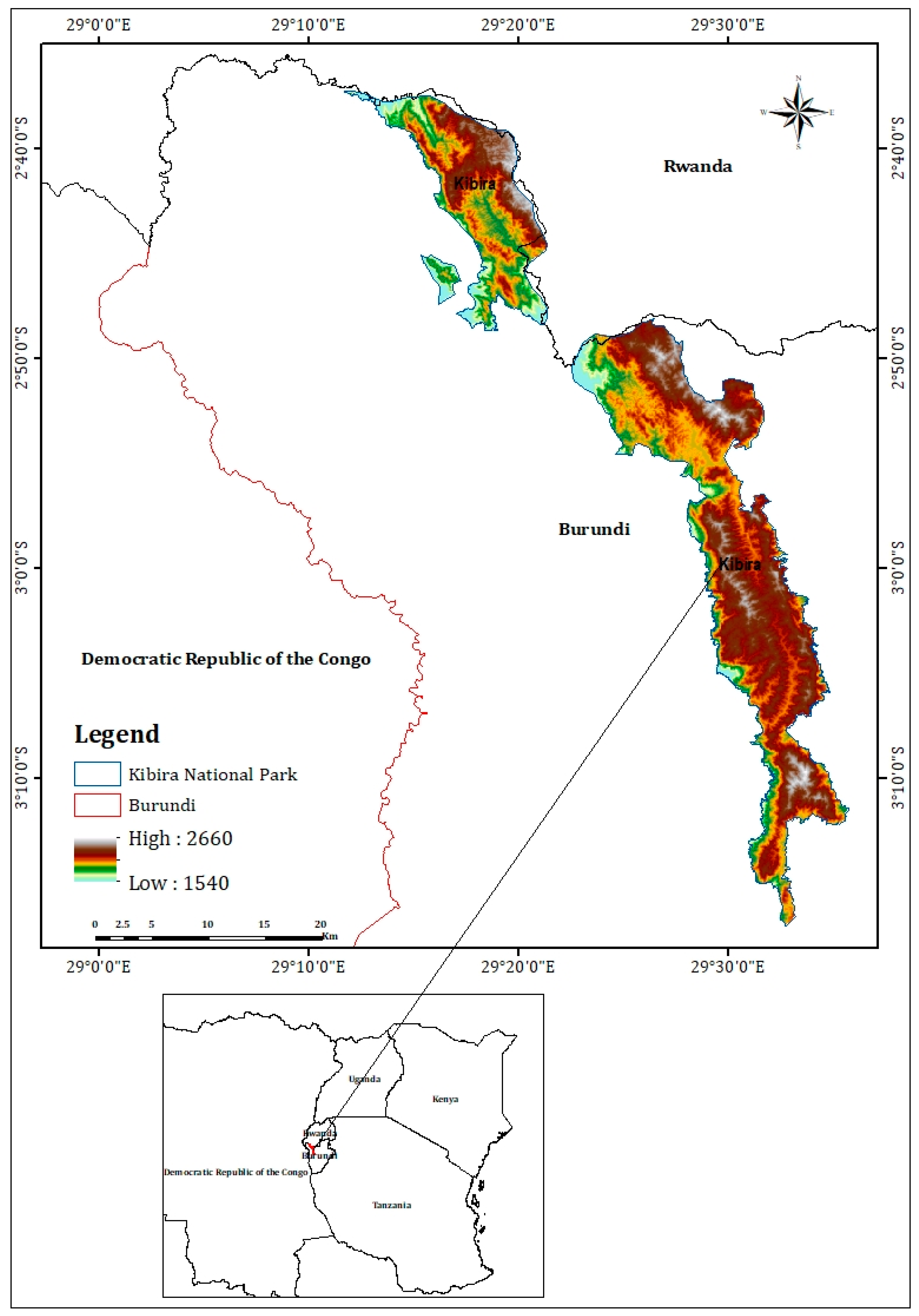
2.1. Study Location

Kibira National Park (Figure 1) is contiguous with Nyungwe National Park, which forms a mountain forest block of 130,000 ha located in northwestern Burundi. Its altitude varies between 1600 and 2666 m [55], covering an approximate area of 427 km². The primary plant species are found in the higher-canopy forest and are dominated by Polyscias fulmar, Entandrophragma excelsum, Macaranga kilimandscharica Parinari excelsa, Syzygium parvifolium, Hagenia abyssinica, and African bamboo (Sinarundinaria Alpina) [25,56], and there is fog vegetation at high altitudes. There is a small evergreen fragment patch at Kigwena, which lies at an altitude of 780–800 m. The temperature in the region is typically cool throughout the year, with an annual rainfall ranging between 1700 and 2000 mm. The park experiences a long dry season from July to August and a short dry season from January to February. This park provides two thirds of the water for Burundi’s hydroelectric energy [57]. During the civil war, the park experienced intensive degradation [22,58], in addition to harvesting dead bamboo and trees. During the El Niño period, the park was affected by fire outbreaks [59]. The adjacent population density is approximately 450 people/km², and this population depends on rain-fed agriculture (potatoes, wheat, beans, and maize) on small parcels of land (generally less than 2 ha) and livestock preserved by zero-grazing within their parcels. Tourism is inadequate due to past insecurity and ongoing uncertainty [60]. In the management process, Kibira was created as a hunting reserve for the King of Burundi and became a forest reserve in 1933, when logging was allowed. Currently, there are restrictions on various local livelihood activities within the park [61]. Between 1980 and 1993, it became a national park; logging and habitation within the park were prohibited. Since 1982, there has been zoning development and an improvement in tourism. From 1995 to 2000, it was classified as the Congo Nile Ridge Forest Reserve and was declared to be Kibira National Park. From 2007 to 2010, transboundary management was signed and communities were mobilized for conservation actions.

2.2. Data Sources

2.2.1. Data for Land Use/Land Cover Change

Remotely sensed data from Landsat 5 Thematic mappers (TMs) and Landsat 8 Operational Land Images (OLIs) were obtained from the United States Geological Survey (USGS) website (https://earthexplorer.usgs.gov/, accessed on 24 January 2023 at a 30 m spatial resolution). This study utilized Landsat 5 TM images from the years 1990, 1994, 2000, and 2011 and Landsat 8 OLIs from the years 2016 and 2021. The scene path and row values for all images were 173 and 62, respectively, and the cloud coverage was less than 10%. All images were level-1 products and were projected onto the Universal Transverse Mercator (UTM) grid using the WGS-84 datum. To ensure high-quality datasets, the overlay technique of geometry correction was applied to mask cloud patches, and atmospheric corrections were made to eliminate haze and aerosol contamination [62]. To minimize the impact of seasonal differences in vegetation phenology between study periods, image scenes were downloaded with similar satellite overpass times or seasons. Specifically, the dry periods ranging from January to February and from July to August were chosen to reduce cloud cover and ensure consistency between the images used in this study.

2.2.2. Landscape Fragmentation Metrics

According to McGarical and Marks et al. [63], we used FRAGSTATS v. 3.3 to quantify five landscape metrics, including the patch density (PD), edge density (ED), largest patch index (LPI), Shannon diversity index, and contagion (CONTAG). These metrics provide indications of the physical fragmentation [64], the diversity richness [65], and the degree of clumping of the attributes [66], respectively (

Table 1. A summary of the landscape metrics used to analyze the relationship with EPI.

Names	Category	Definition
Patch density (PD)	Component of patch	An evaluation of the total number of patches per unit area. It is enhanced as the level of heterogeneity increases.
Number of patches (NP)	Complexity of patch	The number of patches over the entire landscape area.
Largest patch index (LPI)	Patch component	The largest patch index is the largest patch area (m2) in the landscape divided by the total landscape area (m2). This metric decreases as the heterogeneity of the landscape increases.
Edge density (ED)	Patch complexity	Describes the sum of the lengths (m) of all edge segments in the landscape divided by the total study area. As the heterogeneity decreases, the edge density also decreases.
Shannon diversity index (SHDI)	Diversity	Refers to the proportional richness of each patch type, which increases with an increase in abundance.
Contagion (CONTAG)	Configuration	Reflects all types of patches existing in a landscape and is affected by both the interspersion and dispersion of patch types. As the heterogeneity of the landscape increases, the contagion metric decreases.

Source: provided by McGarigal et al. [63].

). The fragmentation index was measured at the landscape level based on the land use type and then compared to the trends between the 1990, 1994, 2000, 2011, 2016, and 2021 periods.

2.2.3. Determinants of Socioeconomic and Demographic Factors

According to White and St. John et al. [67], socioeconomic factors are used to track the progress and social transformation of people’s livelihoods, while demography refers to population growth [68]. Kroll and Haase [69] indicated that factors such as the added GDP from the agriculture, fishery, and forestry industries and the GDP per year characterize the progress in the economy. The main selected demographic aspects include the rural population, which indicates the proportion of residents located in rural areas; urban growth per year, which identifies the percentage by which the inhabitants increases per year in urban regions; and population growth per year, which defines the average increase for the entire country’s population. These factors were provided by the World Development Indicators (WDIs). They are expressed annually as percentages (

Table 2. The selected socioeconomic and demographic factors were used as explanatory variables in the multivariate analysis of variance model (MANOVA).

Abbreviation	Description	Unit	Source
PGY	Population growth per year	% of total population growth per year	WDIs
GDP	Gross domestic product per year	% of total national gross domestic product per year	WDIs
Added/GDP	Gross domestic product added by agriculture, forestry, and fishing	% of total gross domestic product added by agriculture, forestry, and fishing	WDIs
Rul pop	Rural population	% of the total rural population	WDIs
Urb pop	Urban population growth per year	% of total urban population growth	WDIs

Source: author’s compilation from WDI database.

) and are presented at the national (Burundi) level from 1990 to 2021 [70].

2.2.4. Environmental Performance Index

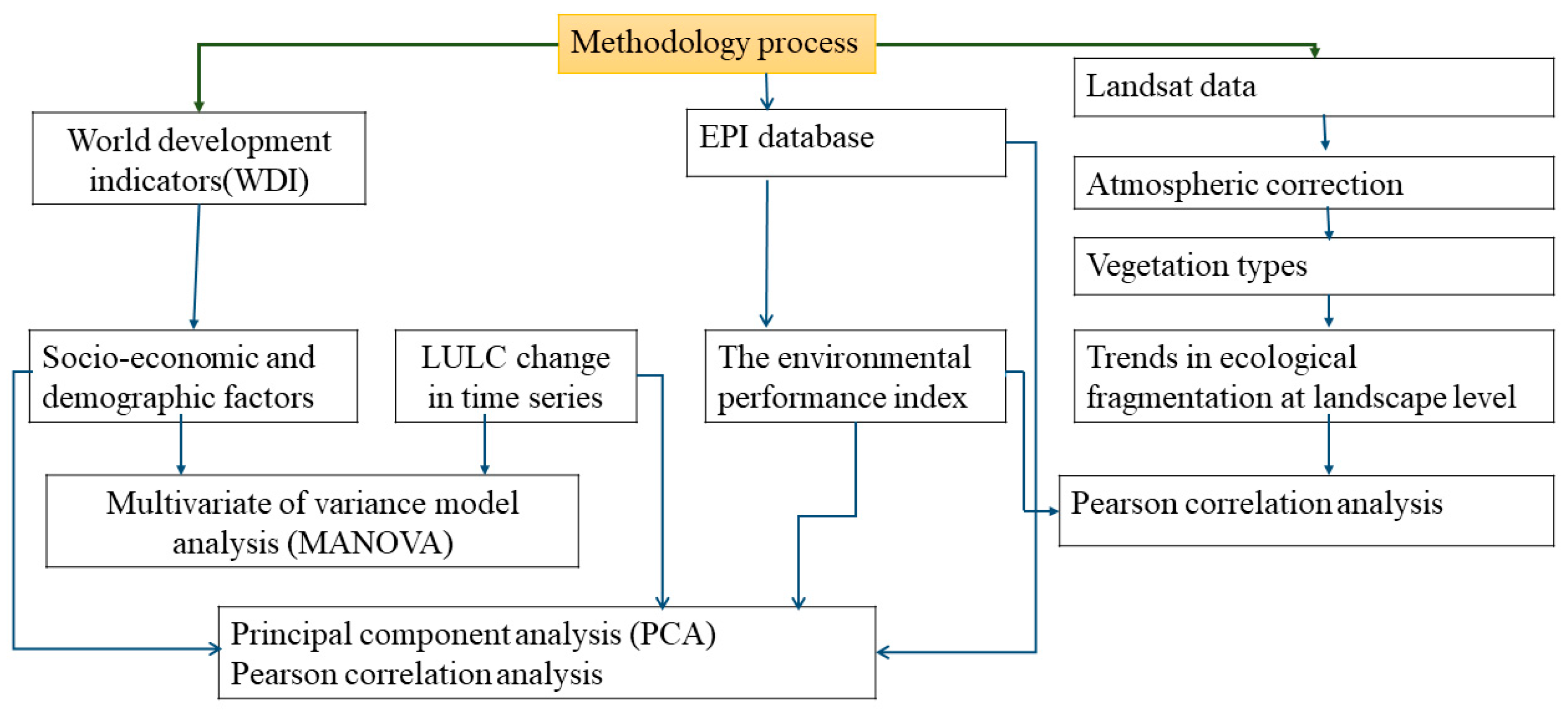
The Yale Center for Environmental Law and Policy (YCELP) developed the environmental performance index (EPI) in 2020, which measures performance across 180 countries based on two objective policies for environmental health and ecosystem vitality and provides a data-driven summary of sustainability with 32 performance indicators across 11 issue categories [71]. The environmental performance index (EPI) is a generated weighted composite index that evaluates various fields by mathematically quantifying and designating the implementation of a state’s policies. Using a target proximity technique, each nation is given a performance score with a value between 0 and 100. The comparatively higher values, which are closer to 100, indicate correctness in performance policy concerns [34]. In this study, from the EPI objectives, the policy objective of ecosystem vitality was selected, particularly biodiversity and habitat, and ecosystem services, to assess its impact on landscape fragmentation using a Spearman correlation analysis. The indicators from 1995 to 2020) are presented in Figure 2 (1 to 26). These indicators include the species protection index (PSI), species habitat index (SHI), Terrestrial Biome Protection (TBN), and Protected Areas Representativeness Index (PAR), as well as indicators related to ecosystem services such as the tree cover loss (TCL), grassland loss (GRL), and wetland loss (WTL). The 2020 EPI presents the results of process indicators, which are scored from 0 to 100. It is specifically available in the Environmental Performance Index, 2020, released by Environmental Performance Index (EPI) | Socioeconomic Data and Application Center (SEDAC) [72].

2.3. Methodology

2.3.1. The Classification of Land Use and Land Cover

Based on Figure 3, one of the frequently used parametric classifiers for supervised classification that accounts for the variance and covariance within class distributions and for data with normal distributions is the maximum likelihood algorithm [73]. With the aid of ArcGIS 10.8, training areas were created by selecting one or more polygons for each class. Then, land use and land cover types were determined by integrating GIS technology based on remote sensing images for the years 1990, 1994, 2000, 2011, 2016, and 2021. We performed a Kappa and accuracy analysis to determine if a land use/land cover category was meaningfully classified [74]. Using ground truth points randomly selected from all land use types, the overall accuracy and Kappa proportions were determined [75]. To evaluate and verify the produced LULC data, 150 random points and tested values from the global imagery were employed, along with estimations of the overall accuracy and Kappa coefficients. For 1990, 1994, 2000, 2011, 2016, and 2021, respectively, the overall accuracies were 0.87, 0.93, 0.90, 0.87, 0.91, and 0.88, while the Kappa factors were 0.84, 0.91, 0.88, 0.84, 0.83, and 0.86. Changes in land use were detected after classification [76].

2.3.2. Multivariate Analysis Model

According to Krzanowski et al. [77], a multivariate analysis concurrently deals with a realistically large number of measurements made for each purpose in one or more samples. A multivariate analysis of variance (MANOVA), specifically, is an analysis of variance that has two or more dependent variables [78]. A multivariate analysis of variance (MANOVA) determines if a response variable is altered by the observer’s manipulation of the independent aspects [43]. Due to a large number of predictors, a MANOVA is efficient in analyzing the relationships between multiple predictors and a dependent variable (response) by assessing the effectiveness of the independent variables for each predicted variable. This method extends simple linear regression, which deals with a single predictor and one dependent variable. This study aimed to determine the impact of different socioeconomic and demographic variables, including the population growth per year; GDP growth rate; added GDP from agriculture, forestry, and fishing; proportion of the rural population; and urban population growth per year, as predictors extracted at the national level. The predicted variables (dependent variables) were the change in LCLU, mainly in forestland, grassland, open land, and water bodies, for Kibira National Park. The proportions of change from 1990 to 1994, from 1994 to 2000, from 2000 to 2011, from 2011 to 2016, and from 2016 to 2021 were kept constant to analyze the impact of socioeconomic and demographic factors from 1990 to 2021, as summarized in Figure 4. Thereafter, during the interpretation of the findings, the coefficients, significance levels, and other relevant statistics were taken into consideration to determine the relationships between the variables.

2.3.3. Spearman Correlation Analysis

A Spearman correlation, also known as a Spearman’s rank correlation coefficient (Spearman’s rho), is a statistical measure used to evaluate the strength and direction of a monotonic relationship between two variables [79]. A Spearman correlation is suited for both linear and non-linear monotonic correlations, unlike a Pearson correlation, which only evaluates linear relationships [80]. In a Spearman correlation analysis, the two variables of interest should be ordinal, interval, or ratio data, as a Spearman correlation is not appropriate for nominal data. In this study, we related the index values of the environmental performance indicators and the values of the index of the landscape fragmentation metrics. A positive Spearman correlation (ρ > 0) indicates a monotonic positive relationship (as one variable increases, the other tends to increase), while a negative Spearman correlation (ρ < 0) indicates a monotonic negative relationship (as one variable increases, the other tends to decrease). A Spearman correlation of 0 (ρ = 0) suggests no monotonic relationship when two variables are not correlated. A Spearman correlation coefficient (ρ) is calculated using the following formula:

$$\rho =1-\frac{6\sum d^2}{n\left(n^2-1\right)}$$

(1)

where ρ is the Spearman correlation coefficient, Σ represents the sum, d represents the differences between the ranks of corresponding data points, and n is the number of data points.

3. Results

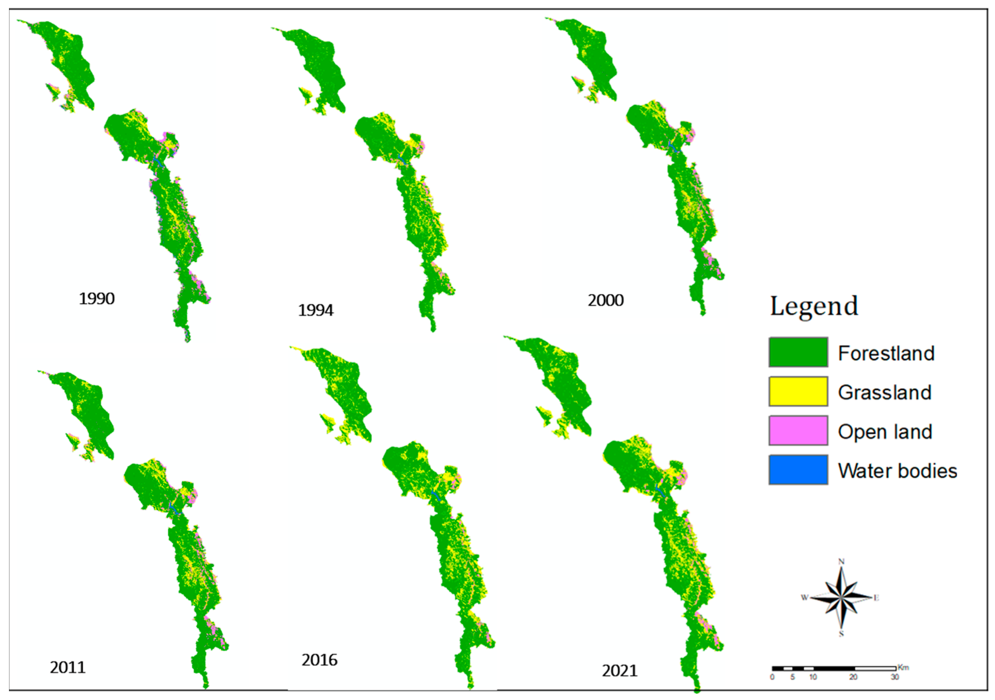
3.1. Transition of Land Use/Land Cover Matrix

The primary vegetation types in Kibira National Park are forestland, grassland, open land, and water bodies, according to the results of the supervised classification (Figure 5).

When comparing the changes shown in Figure 6a,b between 1990 and 1994, open land and water bodies decreased from 2.124% to 1.69% and from 0.352% to 0.217%, respectively, while forestland decreased from 86.1% to 84.62% and grassland expanded from 11.43% to 13.47%. From 1994 to 2000, forestland and open land were reduced to 84.41% and 0.949%, while grassland and water increased to 14.4% and 0.239%. From 2000 to 2011, forestland and water were reduced to 84.1% and 0.224%, while open land and grassland increased again to 1.531% and 14.24%, respectively. From 2011 to 2016, forestland and open land were reduced to 83.35% and 0.593%, while grassland and water bodies increased to 15.83% and 0.23%, respectively. From 2016 to 2021, forestland and water were reduced to 81.32% and 0.178%, while grassland and open land increased to 17.37% and 1.13%. Between 1990 and 2021, forestland, open land, and water bodies were reduced by 4.78%, 0.99%, and 0.171%, whereas grassland increased by 5.94%. Various human influences contributed to the declines in open land, water, and forestland. However, the increase in grassland might be attributable to both conservation efforts and rainfall’s ability to promote vegetation regeneration.

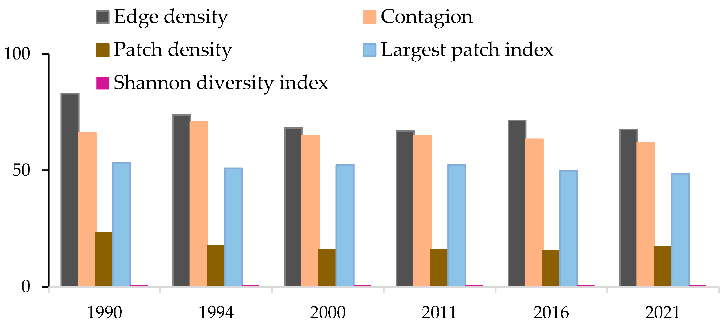
3.2. Transition in Landscape Fragmentation

After computing the fragmentation, Figure 7 shows the index of each landscape metric from 1990 to 2021. Considering the changes from 1990 to 1994, the landscape fragmentation was reduced in the edge density (ED) from 83.35 to 73.879, in the patch density (PD) from 23.03 to 17.76, in the number of patches (NP) from 11,031 to 8493, in the largest patch index (LPI) from 53.19% to 50.85%, and in the Shannon diversity index (SHDI) from 0.7 to 0.66, while the contagion (CONTAG) increased from 65.99% to 70.7%. From 1994 to 2011, the CONTAG, PD, NP, LPI, ED, and SHDI were reduced to 64.84%, 16.05, 7675, 52.43%, 66.97, and 0.61, respectively. In 2016, the fragmentation increased again in the CONTAG, LPI, and ED, which increased to 63.34%, 49.82%, and 71.45, while the fragmentation was reduced in the NP, PD, and SHDI by 15.50, 7452, and 0.65, respectively. In 2021, the landscape fragmentation increased again in the CONTAG, LPI, SHI, PD, and NP by 61.84%, 48.46%, 0.63, 17.08, and 8165, respectively, while the ED decreased to 67.54. Note that the reductions in LPI and CONTAG denoted a fragmentation increase, while the increases in NP and PD denoted an increase. Generally, in 2011 there was a fragmentation reduction compared to 1990; however, an increase started again in 2016 and 2021, denoting enduring negligible human threats within the park.

3.3. Spearman Correlation between EPI and Landscape Fragmentation

The statistically significant correlation coefficient results between the environmental performance indexes and landscape fragmentation metrics, set at a 5% level, are presented in

Table 3. The results of Spearman correlation coefficients between environmental performance indexes and fragmentation metrics.

		ED	CONTAG	NP	PD	SHDI	SHI	SPI	BHI	NTB	PAR	TCL	GRL	WTL	LPI
ED	Pearson Correlation	1	−0.315	−0.050	−0.050	0.017	−0.774 **	0.599 *	−0.458	0.685 **	0.519	−0.636 *	0.379	−0.075	−0.907 **
	Sig. (2-tailed)		0.294	0.870	0.870	0.957	0.002	0.031	0.115	0.010	0.069	0.020	0.202	0.808	0.000
	N	13	13	13	13	13	13	13	13	13	13	13	13	13
CONTAG	Pearson Correlation	−0.315	1	0.597 *	0.597 *	0.916 **	0.766 **	−0.642 *	0.664 *	−0.390	−0.695 **	0.689 **	0.611 *	0.942 **	0.703 **
	Sig. (2-tailed)	0.294		0.031	0.031	0.000	0.002	0.018	0.013	0.188	0.008	0.009	0.027	0.000	0.007
	N	13	13	13	13	13	13	13	13	13	13	13	13	13	13
NP	Pearson Correlation	−0.050	0.597 *	1	1.000 **	0.783 **	0.374	−0.332	0.400	−0.087	−0.402	0.128	0.654 *	0.773 **	−0.059
	Sig. (2-tailed)	0.870	0.031		0.000	0.002	0.208	0.268	0.176	0.778	0.174	0.677	0.015	0.002	0.849
	N	13	13	13	13	13	13	13	13	13	13	13	13	13	13
PD	Pearson Correlation	−0.050	0.597 *	1.000 **	1	0.783 **	0.374	−0.332	0.400	−0.087	−0.402	0.128	0.654 *	0.773 **	−0.059
	Sig. (2-tailed)	0.870	0.031	0.000		0.002	0.208	0.268	0.176	0.778	0.174	0.677	0.015	0.002	0.849
	N	13	13	13	13	13	13	13	13	13	13	13	13	13	13
SHDI	Pearson Correlation	0.017	0.916 **	0.783 **	0.783 **	1	0.520	−0.456	0.536	−0.148	−0.544	0.422	0.815 **	0.992 **	−0.755 **
	Sig. (2-tailed)	0.957	0.000	0.002	0.002		0.069	0.117	0.059	0.629	0.054	0.150	0.001	0.000	0.003
	N	13	13	13	13	13	13	13	13	13	13	13	13	13	13
SHI	Pearson Correlation	−0.774 **	0.766 **	0.374	0.374	0.520	1	−0.890 **	0.864 **	−0.494	−0.905 **	0.860 **	0.166	0.615 *	0.637 *
	Sig. (2-tailed)	0.002	0.002	0.208	0.208	0.069		0.000	0.000	0.086	0.000	0.000	0.588	0.025	0.019
	N	13	13	13	13	13	13	13	13	13	13	13	13	13	13
SPI	Pearson Correlation	0.599 *	−0.642 *	−0.332	−0.332	−0.456	−0.890 **	1	−0.854 **	0.221	0.883 **	−0.693 **	−0.122	−0.549	0.569 *
	Sig. (2-tailed)	0.031	0.018	0.268	0.268	0.117	0.000		0.000	0.468	0.000	0.009	0.691	0.052	0.042
	N	13	13	13	13	13	13	13	13	13	13	13	13	13	13
BHI	Pearson Correlation	−0.458	0.664 *	0.400	0.400	0.536	0.864 **	−0.854 **	1	−0.208	−0.995 **	0.792 **	0.332	0.636 *	0.528
	Sig. (2-tailed)	0.115	0.013	0.176	0.176	0.059	0.000	0.000		0.496	0.000	0.001	0.267	0.019	0.064
	N	13	13	13	13	13	13	13	13	13	13	13	13	13	13
NTB	Pearson Correlation	0.685 **	−0.390	−0.087	−0.087	−0.148	−0.494	0.221	−0.208	1	0.234	−0.555 *	0.084	−0.187	−0.646 *
	Sig. (2-tailed)	0.010	0.188	0.778	0.778	0.629	0.086	0.468	0.496		0.441	0.049	0.785	0.542	0.017
	N	13	13	13	13	13	13	13	13	13	13	13	13	13	13
PAR	Pearson Correlation	0.519	−0.695 **	−0.402	−0.402	−0.544	−0.905 **	0.883 **	−0.995 **	0.234	1	−0.814 **	−0.307	−0.646 *	−0.537
	Sig. (2-tailed)	0.069	0.008	0.174	0.174	0.054	0.000	0.000	0.000	0.441		0.001	0.307	0.017	0.058
	N	13	13	13	13	13	13	13	13	13	13	13	13	13	13
TCL	Pearson Correlation	−0.636 *	0.689 **	0.128	0.128	0.422	0.860 **	−0.693 **	0.792 **	−0.555 *	−0.814 **	1	0.148	0.513	0.625 *
	Sig. (2-tailed)	0.020	0.009	0.677	0.677	0.150	0.000	0.009	0.001	0.049	0.001		0.630	0.073	0.022
	N	13	13	13	13	13	13	13	13	13	13	13	13	13	13
GCL	Pearson Correlation	0.379	0.611 *	0.654 *	0.654 *	0.815 **	0.166	−0.122	0.332	0.084	−0.307	0.148	1	0.782 **	−0.715 **
	Sig. (2-tailed)	0.202	0.027	0.015	0.015	0.001	0.588	0.691	0.267	0.785	0.307	0.630		0.002	0.006
	N	13	13	13	13	13	13	13	13	13	13	13	13	13	13
WTL	Pearson Correlation	−0.075	0.942 **	0.773 **	0.773 **	0.992 **	0.615 *	−0.549	0.636 *	−0.187	−0.646 *	0.513	0.782 **	1	0.644 *
	Sig. (2-tailed)	0.808	0.000	0.002	0.002	0.000	0.025	0.052	0.019	0.542	0.017	0.073	0.002		0.017
	N	13	13	13	13	13	13	13	13	13	13	13	13	13	13
LPI	Pearson Correlation	−0.907 *	0.703 **	−0.059	−0.059	−0.755 **	0.637 *	0.569 *	0.528	−0.646 *	−0.537	0.625 *	−0.715 **	0.644 *	1.000
	Sig. (2-tailed)	0.000	0.007	0.849	0.849	0.003	0.019	0.042	0.064	0.017	0.058	0.022	0.006	0.017
	N	13	13	13	13	13	13	13	13	13	13	13	13	13	13

** Correlation is significant at the 0.01 level (2-tailed). * Correlation is significant at the 0.05 level (2-tailed).

. For instance, there was a significant strong positive correlation between the edge density (ED), NTB, and SPI, whereas there was a negative correlation between the ED, SHI, and TCL. Also, the CONTAG metric was strongly and significantly correlated with the SHI, BHI, TCL, GRL, and WTL, whereas there was a significant negative correlation between the CONTAG, SPI, and PAR. Moreover, the NP and PD were strongly, positively, and significantly correlated with the GRL and WTL. Furthermore, the SHDI was positively and significantly correlated with the GRL and WTL. There was a significant correlation between increases in the fragmentation metric and the performance of the EPI aimed at ecosystem services, implying a severe exploitation of natural resources.

3.4. Impact of Socioeconomic and Demographic Factors on LCLU Changes

By applying a multivariate analysis of variance (MANOVA) to assess the influence of socioeconomic and demographic factors on changes in land cover (LCLU), the model’s fitness determined that the vegetation types (grasslands, forests, open spaces, and water bodies) had correlation coefficients of 0.3, 0.4, 0.2, and 0.3, respectively (

Table 4. Summary of the fitness of the MANOVA model.

Equation	Observations	Number of Independent Variables	Route-Mean-Square Error	R2	Value	p-Value
Forestland	31	5	0.6	0.3	2.25	0.0804
Grassland	31	5	0.8	0.4	3	0.0338
Open land	31	5	0.6	0.2	2.1	0.1057
Water bodies	31	5	0.05	0.3	1.7	0.1725

). Additionally, as shown in

Table 5. Results of MANOVA model for socioeconomic and demographic predictors of LCLU changes.

Years	Coefficient	Std. Err.	T	p > t
PGY	1.083	1.808	0.6	0.554
GDP	−0.039	0.101	−0.39	0.701
Added/GDP	−0.006	0.084	−0.07	0.946
Rul pop	−3.964	0.194	−20.39	0.000 *
Urb pop	−0.758	1.795	−0.42	0.676
_cons	2364.908	14.939	158.3	0.000
Forestland
PGY	0.983	0.655	1.5	0.146
GDP	0.016	0.037	0.45	0.657
Added/GDP	−0.022	0.030	−0.74	0.465
Rul pop	0.190	0.070	2.7	0.012 *
Urb pop	−0.855	0.650	−1.31	0.200
_cons	−16.157	5.414	−2.98	0.006
Grassland
PGY	−2.056	0.764	−2.69	0.012 *
GDP	−0.073	0.043	−1.72	0.098
Added/GDP	0.035	0.035	1	0.328
Rul pop	−0.200	0.082	−2.43	0.022 *
Urb pop	1.851	0.758	2.44	0.022 *
_cons	14.779	6.308	2.34	0.027
Open
PGY	0.979	0.660	1.48	0.150
GDP	0.060	0.037	1.62	0.117
Added/GDP	−0.014	0.031	−0.45	0.657
Rul pop	0.008	0.071	0.11	0.912
Urb pop	−0.915	0.655	−1.4	0.175
_cons	1.357	5.455	0.25	0.805
Water bodies
PGY	0.094	0.053	1.79	0.085
GDP	−0.003	0.003	−1.04	0.306
Added/GDP	0.001	0.002	0.42	0.680
Rul pop	0.001	0.006	0.26	0.793
Urb pop	−0.082	0.052	−1.57	0.129
_cons	0.020	0.435	0.05	0.963

Note: * represents significance at 5% level.

, the model showed that, at the 5% level, with a p-value of 0.000, the percentage of the rural population had the largest significant impact on changes in land use and land cover. Forestland and grassland were impacted by the rural population with p-values of 0.012 and 0.022, respectively. Grassland was impacted by variables such as the annual population growth and urban population, with p-values of 0.012 and 0.022, respectively. Furthermore, the model found that, at 10% significance, the GDP and annual population increase had a minor impact on changes in grasslands and water bodies, with respective p-values of 0.098 and 0.085. In general, the socioeconomic variables had a small impact on the changing LCLU, while the demographic indicators had a stronger impact.

3.5. The Principal Component Analysis Results

After connecting various indicators, such as the EPI, socioeconomic and demographic parameters, and LCLU changes based on a principal component analysis (PCA),

Table 6. Results from the principal component analysis (PCA) with eigenvalues greater than one.

	PC1	PC2	PC3	PC4
Years	−0.0746	−0.0774	−0.1319	0.008
Forestland	−0.1694	0.1799	0.024	117
Grassland	0.3672	−0.0702	0.0091	−0.0046
Open land	−0.2997	−0.1231	−0.034	−0.0047
Water bodies	−0.1445	0.451	−0.0252	−0.0127
PGY	0.4957	0.1632	0.706	0.0219
GDP	−0.242	−0.0738	0.0057	−0.0008
Added GDP	−0.3334	0.5045	0.0172	0.0013
Rul pop	0.0887	0.0961	0.0383	−0.0002
Urb Pop	0.5385	0.1812	−0.6746	−0.0195
SHI	0.039	0.5146	0.0485	0.0124
SPI	0.0379	0.2601	−0.0547	0.6627
BTN	0.0174	−0.0864	0.0574	−0.0015
PAR	−0.0549	−0.1511	0.127	0.1079

displays four components with eigenvalues larger than one. PC1 represents the annual population increase, urban population, and water bodies. PC2 represents the species habitat index (SHI) and the added value of the GDP from agriculture, fishing, and forestry. PC4 simply displays the species protection index (SPI), while PC3 displays both the annual and urban population increases. When compared to other metrics, the contribution of demographic factors is highly suggestive.

3.6. The Pearson Correlation Results

Table 7. Pearson correlation coefficients (R²) between the socioeconomic and demographic factors, EPI, and LCLU changes.

Variables	Years	Forestland	Grassland	Open Land	Water	PGY	GDP	Added GDP	Rul Pop	Urb Pop	SHI	SPI	BTN	PAR
	1
Forestland	−0.3	1
Grassland	−0.05	−0.66	1
Open land	0.34	−0.19	−0.61	1
Water	0.31	0.72	−0.51	−0.1	1
PGY	0.38	0.2	−0.47	0.38	0.36	1
GDP	0.3	0.002	−0.3	0.39	0.01	0.47	1
Added GDP	0.18	−0.26	0.19	0.2	−0.1	0.42	0.5	1
Rul Pop	−0.99	0.34	0.002	−0.3	−0.3	−0.3	−0.3	0.19	1
Urb Pop	0.3	0.21	−0.44	0.34	0.31	0.99	0.47	0.06	−0.3	1
SHI	−0.46	−0.36	0.34	−0.05	−0.4	−0.5	−0.44	−0.02	0.43	−0.45	1
SPI	0.68	−0.71	0.35	0.27	−0.1	0.01	−0.01	0.23	−0.7	−0.04	0.3	1
BTN	0.92	−0.42	0.18	0.17	0.17	0.28	0.23	0.27	−0.9	0.21	−0.42	0.7	1
PAR	0.96	−0.38	−0.07	0.45	0.15	0.42	0.37	0.19	−1	0.35	−0.43	0.7	0.9	1

displays the results of the Pearson correlation. There was a negative connection of 0.7 between forestland and the SPI and a substantial positive coefficient of 0.72 between forestland and water bodies. There was a negative correlation between grassland and water of 0.51. Additionally, there was a moderate association of 0.51 between PGY and open land. Open land contributed to GDP and had a moderate relationship with PGY and GDP. The annual gross domestic product (GDP) of the country was positively associated (0.5) with the additional GDP from agriculture, fishing, and forestry. The percentage of people living in cities was substantially correlated with PGY (0.99). The rural population exhibited strong negative correlations with SPI and BTN, with respective values of 0.7 and 0.9. Conversely, there was a positive correlation between biodiversity and habitats. There were significant connections among similarly categorized variables, which favors the implementation of measures.

4. Discussion

4.1. Land Use/Land Cover Change

As can be seen in Figure 5 and Figure 6, from 1990 to 2021 there was a dramatic decrease in forestland. Intensive deforestation occurred before strengthening the protection measures, in addition to the civil war, which occurred between 1993 and 2005, and the exploitation of bamboo along the northwestern part of the park [25,28]. Comparatively, Kayiranga et al. [24] also proved that Kibira National Park is currently experiencing a forestland reduction of about 0.27% per year when employing a comparable classification method. These findings are consistent with an earlier study that applied a similar technique to generalize vegetation types and their changes, where the forestland was the largest component and had been significantly reduced between 2000 and 2013 [81]. Our findings are in line with a study by Escobedo et al. [82], who discovered that socioeconomic human activities often cause the direct loss and conversion of land, which have further negative impacts on the landscape’s structure and configuration and on biodiversity functions. On the other hand, grassland increased between 1990 and 2021, as can be seen in Figure 6a,b, which led to vegetation renewal and the conversion of other kinds of ecosystems. We can infer that open land was changed to grassland, as it decreased from 2.124% to 1.134%, showing that an effort was made by the park management (Figure 5). These results are consistent with those of Schmitz et al. [83], who quantified the extent of land use dynamics driven by local socioeconomic activities and revealed a land loss balanced with the extent of conservation actions. They also found that regional protection led to significant ecological restoration in shrubland. Moreover, the results show that water bodies decreased between 1990 and 2021, as presented in Figure 6b. This was due to the intensive application of different socioeconomic activities, including irrigation in agriculture, fishing, and hydroelectricity [25]. Therefore, to inform land use managers, a first attempt to quantify the alteration in LULC is necessary to address every type of human threat connected with each type of vegetation. Taking into account how the climate affects the distribution of vegetation, variations in altitude cause precipitation to be redistributed, which in turn supports the redistribution of land use and land cover [84]. For instance, in Rwanda, a decline in rainfall amounts was correlated with a reduction in terrain [85]. The distribution of dense forestlands along the western ridge of Kibira National Park (Figure 5), which is shown at a lower height (Figure 1), is consistently explained by the topography–rainfall relationship. The northern–eastern altitude ridge is distributed in dense grasslands (Figure 5), in contrast to the western zone (Figure 1). For example, research by Wang et al. [86] revealed that the distribution of grasslands is most affected by annual rainfall above 600 mm. In the Congo–Nile divide, where Kibira National Park is located at an elevation of 1700 to 2500 mm on a steep slope with an average precipitation range of 1300 to 2000, a comparable, intense grassland distribution was discovered [87]. The grassland areas were improved in 2021 compared to the earlier years. This enhancement reacted to rising precipitation as well as the regrowth of vegetation in open spaces. An analogous study conducted in Rwanda for Nyungwe National Park showed that when precipitation is predicted to increase, this leads to an increase in grassland cover while forest cover continues to decline [88]. Understanding how climate and topography affect vegetation distribution may aid in predicting the effects of future climatic changes on the distribution of various ecosystems.

4.2. Analysis of the Landscape Fragmentation

The results from the landscape fragmentation metric calculation showed that the contagion metric was reduced from 1990 to 2021 (Figure 7), denoting degradation and weak connectivity. Generally, a high value that tends to 100% shows that there is a certain dominant patch type in the landscape, which implies good connectivity; a lower value (tends to 0) indicates a dense landscape pattern with numerous patches and a degree of fragmentation that is fairly high [66,89]. The number of patches as well as the patch density were reduced in 2011 and 2016; however, in 2016, the fragmentation started to increase, and this continued in 2021, as presented in Figure 7. The edge density was high in 1990 and decreased in 2021, denoting the eradication of degradation in the park boundaries. Our findings are consistent with a study by Ma et al. [90], who assessed the impact of high edge density on plant richness in agricultural landscapes. This research discovered that the level of edge density in non-agricultural boundary areas surrounded by usable lands has a significant impact on the loss of diversity. In addition, this study found that the species richness index (SHDI) decreased moderately between 1990 and 2021. The reduction in the SHDI indicates diversity loss due to natural and negligible human threats that may have occurred within the park, both before and after implementing the control measures. The largest patch index (LPI) decreased between 1990 and 2021, leading to increasing fragmentation. Li et al. [91] denoted a reduction in the LPI value from 21.41% to 4.42% during the study period as a result of green space reduction, which resulted in higher fragmentation. In general, the landscape fragmentation metrics did not show large reductions, and the management efforts still needed to succeed in sustaining biodiversity within and at the edges of the park. Fragmentation evaluation is essential for understanding how ecological systems reflect the challenges of land use change and utilization and to acknowledge efforts made by conservationists to alleviate threats to biodiversity.

4.3. Relationship between Environmental Performance Index and Landscape Fragmentation

Table 3 presents the outcomes of a Spearman correlation analysis, which shows the impact of environmental performance index (EPI) indicators for national objectives aimed at ecosystem vitality (Figure 2) on the trends in landscape fragmentation metrics (Figure 7). There is a strong and statistically significant correlation between the park’s edge density index and EPI indicators such as the species protection index (SPI) and Terrestrial Biome Protection (BTN). Furthermore, it can be noted that the SPI and BTN lead to reductions in edge density degradation, as evidenced by the decrease in edge density (ED) in 2021 (Figure 7). In this situation, we can agree that the extent of management actions may contribute to the greater or weaker significance of biodiversity [92]. This is because other indicators such as tree cover loss (TCL) and the species habitat index (SHI) exhibit strong negative correlations, as shown in Figure 2, resulting in a weak performance in mitigating the disturbances effects. These findings are consistent with the conclusions of a previous study conducted by Baltzer et al. [93], which demonstrated that weak conservation has resulted in forestland loss, which denotes fragmentation on the edges of the landscape. The implication of the EPI for edge fragmentation offers an adaptation measure for which the environmental performance aims must consider regional factors that can prioritize the landscape to completely overcome the edge disturbances. Furthermore, the environmental performance index (EPI) indicators targeting the species habitat index (SHI), biodiversity habitat index (BHI), tree cover loss (TCL), grassland loss (GRL), and wetland loss (WTL) were found to be strongly and statistically significantly associated with the contagion metric. These findings are consistent with the conclusions of a previous study conducted by Kuussaari et al. [94], which emphasized the importance of evaluating the effectiveness of protection measures for grasslands, trees, and wetlands in conserving their ecological values. Furthermore, the Shannon diversity index (SHDI) decreased in 2021 and resulted in a strong and statistically significant association between the wetland loss (WTL) and grassland loss (GRL) indicators. These findings are consistent with the conclusions of a study by Lehtinen et al. [95], which suggested that the weak diversity in wetlands is due to patch isolation. Additionally, Wesche et al. [96] confirmed that significant grassland loss is likely to harm species richness. Expectedly, the patterns of landscape metrics such as the contagion, LPI, NP, PD, and SHDI were strongly correlated and showed a significant impact on the EPI aimed at ecosystem services. Based on this, by eradicating the failures of the EPI, which is aimed at ecosystem services (WTL, GRL, and TCL), we can improve ecological connectivity and enhance the value of these habitats. Additionally, we observed strong connections between indicators such as the TCL, WTL, SHI, SPI, and largest patch index, while a negative association was obtained for the grassland cover loss (GRL) and BTN. Integrating the environmental performance index for ecosystem vitality is crucial to addressing trends in landscape fragmentation. Therefore, harmonizing the environmental performance for successful biodiversity is essential to support ecological functions.

4.4. The Impact of Socioeconomic and Demographic Factors on Land Use/Land Cover Change

The results from the multivariate analysis of variance (MANOVA) showed the model’s fitness had an average r-square value (Table 4). These coefficients signify the reduction in collinearity due to the minor factors that may contribute to the changes in the LCLU within the park. Another explanatory variable identified by the MANOVA results is the rural population, which is decreasing by 3.9% annually and has a statistically significant impact (at the 5% level) on the change in land use and land cover (Table 5). This is supported by a study conducted by Lambin et al. [97], who confirmed that through several factors, such as the loss of agricultural land, LULC changes may cause a decline in the population of rural areas. As anticipated, the MANOVA revealed a positive association between the rural population and forestland (Table 5), which is statically significant at the 5% level. As such, rapid rural growth has proven to be linked to extensive agriculture for rural livelihoods and causes scarcity of land via deforestation [98]. Moreover, Carte et al. [99] also found that there was a statistically significant association between reforestation and rural population growth. The residents’ displacement strategy is a crucial policy that allows local inhabitants to be relocated and prohibited from accessing the resources and land that underpin their socioeconomic status [100]. Additionally, the annual population growth and the population of rural areas were linked to an improvement in the grassland. These results were both statistically significant at the 5% level, as presented in Table 5. These results point to an efficient method for restoring grassland that needs the considerable stabilization of population growth. The findings also indicated a positive correlation between urban population growth per year and grassland, as an increase of one unit in urban regions would increase the grassland by 1.85% of the available land reserved for grassland areas. While urbanization upgrades (for instance, enhancing the beauty of park amenities or gardens) might spur economic growth, doing so also serves to enhance green areas and raises the value of ecological aesthetics [101]. The major motivating factors for land use change are demographic patterns; hence, appropriate management strategies need to include the population. On the other hand, throughout the model process, the small variations in LCLU that were noticed did not show statistical significance at the 5% level. Expectedly, a moderate positive coefficient with a statistical significance of 10% was seen when the water body change was associated with the population increase each year (Table 5). These results are supported by Chowdhury et al. [102], who emphasized that water resources are being depleted due to the growing demand from farming, fisheries, electricity, and sanitation. Therefore, it is necessary to implement managerial policies to balance the water usage of various socioeconomic activities. Moreover, controlling actions are required to maintain a balance between water usage and population growth. It was also observed that there was a positive and statistically significant relationship between the annual GDP and grassland, which was significant at the 10% level. These findings are consistent with research conducted by Zhong et al. [103], who showed that the share of the gross domestic product from agriculture in the total GDP fell from 52.26% to 7.3% when the vegetation covering the studied region grew from 40.6% to 78.5%. Future GDP targets linked to socioeconomic goals need to harmonize land utilization. Balancing environmental and social needs requires considering how socioeconomic and demographic factors affect LULC change.

4.5. The Factor Analysis between Macro-Indicators

The relationships that show the most important factors, as presented in Table 6 and Table 7, were obtained after connecting the EPI indicators related to biodiversity and habitat (the SHI, SPI, PAR, and BTN), changes in land use/land cover, and socioeconomic and demographic factors. These highly related factors are generally acceptable for clarifying the important variables that have eigenvalues greater than one [104]. A similar study conducted by Leśniewska-Napierała et al. [105] employed a PCA to examine the association between economic control and demographic, social, infrastructural, institutional, and environmental factors. The findings provided a better explanation of the drivers of changes in land cover. Regarding the Pearson coefficients presented in Table 7, there was a positive relationship between water bodies and forestland, even when both vegetation types had been reduced (Figure 6b). These results are consistent with findings by Asner et al. [106], who showed severe canopy water losses of over 30% occurring across 1 million hectares, resulting in damage to large trees. Furthermore, we can suggest that the population’s expansion consumes large amounts of water, given that a strong correlation was identified (Table 7). Based on PC1 and PC3, annual population growth has a positive connection with urban population growth and the GDP. This association aligns with research by Seto et al. [107], who demonstrated that annual progress in gross domestic product per capita is liable for almost half of the observed urban expansion in Africa. This study also showed that the annual GDP growth was strongly correlated with the added GDP from forestry, fishing, and agriculture. This situation is reasonable given the importance of farming in the country’s GDP contribution [18]. The high population density in rural areas and the dependence on natural resources (forestland) were not positively correlated (Table 7) with the application of the national policies aimed at the SPI and BTN indicators, which search to restore the degraded ecosystem (forestland). However, we still need to make a durable effort to stabilize the park’s diversity in both vegetation types. This will be achieved because the grassland has already regenerated, as evidenced by its increase in Figure 6b and its moderate positive correlation with the SPI (Table 7). It is essential to underline the strongly correlated aspects when evaluating how environmental performance indicators act on biodiversity to control the impact brought by socioeconomic and demographic factors.

5. Conclusions and Implications

This study aimed to assess the impact of socioeconomic and demographic factors on land cover and land use changes. Additionally, this study analyzed the relationship between the environmental performance index (EPI) and metrics of landscape fragmentation. Finally, it revealed the interplay of aspects such as socioeconomic and demographic variables, the EPI, and LULC changes. The reductions in water bodies and forestland suggest the need for robust management measures. Despite controlling measures being implemented to reduce the reduction in edge density fragmentation until 2021, careful control of human threats is suggested due to the increased landscape fragmentation in recent years, given that the rural population was the main demographic indicator significantly impacting the forestland. This study highlights the necessity of aligning reforestation and conservation efforts with the perspectives of rural populations. Furthermore, demographic factors significantly influenced grassland change, while water bodies were moderately affected by annual population expansion. To ensure sustainable biodiversity, a careful emphasis on population control can be considered by land managers aiming at biodiversity restoration success. Furthermore, socioeconomic aspects such as the GDP had moderate impacts. GDP-based natural ecosystem exploitation should be shifted to other commercial sectors to harmonize economic dependence in agriculture. This study also indicated that the EPI aimed at ecosystem services has a direct response to landscape fragmentation, suggesting a need for additional effort to maximize EPI targets related to biodiversity restoration. Positive indicators such as the SPI and NTB were crucial for reducing edge density (ED), highlighting the positive direction of managerial efforts. This study also showed a strong relationship between water bodies and forestland, emphasizing the importance of rigorous policies for future biodiversity protection in both ecosystems. Demographic variables are significantly correlated with annual GDP growth, and the additional GDP from forestry, fishing, and agriculture could provide more economic profits for livelihood needs and could be useful to reduce natural resource exploitation.

This study has some shortcomings that need to be appropriately addressed by subsequent research. One of them is the impacts of LCLU alterations. Future research should take into account some human activities that have been disregarded but are associated with disturbances. Additionally, since this work used a time-series change analysis due to the unavailability of annual Landsat data, limited data availability has been a drawback. Thus, taking these pertinent difficulties into account in future research could improve the tracking of changes aimed at advancing this sector. To harmonize economic changes, a wider cross-sectional examination in many countries and protected regions is required, as this study was conducted only in Kibira National Park, Burundi.

References

1. Verburg, P.H.; Crossman, N.; Ellis, E.C.; Heinimann, A.; Hostert, P.; Mertz, O.; Nagendra, H.; Sikor, T.; Erb, K.-H.; Golubiewski, N. Land system science and sustainable development of the earth system: A global land project perspective. Anthropocene 2015, 12, 29–41. [Google Scholar] [CrossRef]
2. Geist, H.; McConnell, W.; Lambin, E.F.; Moran, E.; Alves, D.; Rudel, T. Causes and trajectories of land-use/cover change. In Land-Use and Land-Cover Change: Local Processes and Global Impacts; Springer: Berlin/Heidelberg, Germany, 2006; pp. 41–70. [Google Scholar]
3. Meshesha, D.T.; Tsunekawa, A.; Tsubo, M.; Ali, S.A.; Haregeweyn, N. Land-use change and its socio-environmental impact in Eastern Ethiopia’s highland. Reg. Environ. Chang. 2014, 14, 757–768. [Google Scholar] [CrossRef]
4. Bren d’Amour, C.; Reitsma, F.; Baiocchi, G.; Barthel, S.; Güneralp, B.; Erb, K.-H.; Haberl, H.; Creutzig, F.; Seto, K.C. Future urban land expansion and implications for global croplands. Proc. Natl. Acad. Sci. USA 2017, 114, 8939–8944. [Google Scholar] [CrossRef] [PubMed]
5. Yirsaw, E.; Wu, W.; Temesgen, H.; Bekele, B. Socioeconomic drivers of spatio-temporal land use/land cover changes in a rapidly urbanizing area of China, the Su-Xi-Chang region. Appl. Ecol. Environ. Res. 2017, 15, 809–827. [Google Scholar] [CrossRef]
6. Ramankutty, N.; Graumlich, L.; Achard, F.; Alves, D.; Chhabra, A.; DeFries, R.S.; Foley, J.A.; Geist, H.; Houghton, R.A.; Goldewijk, K.K. Global land-cover change: Recent progress, remaining challenges. In Land-Use and Land-Cover Change: Local Processes and Global Impacts; Springer: Berlin/Heidelberg, Germany, 2006; pp. 9–39. [Google Scholar] [CrossRef]
7. Wassenaar, T.; Gerber, P.; Verburg, P.H.; Rosales, M.; Ibrahim, M.; Steinfeld, H. Projecting land use changes in the Neotropics: The geography of pasture expansion into forest. Glob. Environ. Chang. 2007, 17, 86–104. [Google Scholar] [CrossRef]
8. Gong, C.; Yu, S.; Joesting, H.; Chen, J. Determining socioeconomic drivers of urban forest fragmentation with historical remote sensing images. Landsc. Urban Plan. 2013, 117, 57–65. [Google Scholar] [CrossRef]
9. Vanacker, V.; Govers, G.; Barros, S.; Poesen, J.; Deckers, J. The effect of short-term socio-economic and demographic change on landuse dynamics and its corresponding geomorphic response with relation to water erosion in a tropical mountainous catchment, Ecuador. Landsc. Ecol. 2003, 18, 1–15. [Google Scholar] [CrossRef]
10. Viglizzo, E.F.; Frank, F.C.; Carreño, L.V.; Jobbagy, E.G.; Pereyra, H.; Clatt, J.; Pincén, D.; Ricard, M.F. Ecological and environmental footprint of 50 years of agricultural expansion in Argentina. Glob. Chang. Biol. 2011, 17, 959–973. [Google Scholar] [CrossRef]
11. Lambin, E.F.; Geist, H.J.; Lepers, E. Dynamics of land-use and land-cover change in tropical regions. Annu. Rev. Environ. Resour. 2003, 28, 205–241. [Google Scholar] [CrossRef]
12. Li, X.; Wang, Y.; Li, J.; Lei, B. Physical and socioeconomic driving forces of land-use and land-cover changes: A Case Study of Wuhan City, China. Discret. Dyn. Nat. Soc. 2016, 2016, 8061069. [Google Scholar] [CrossRef]
13. Bai, Z.G.; Dent, D.L.; Olsson, L.; Schaepman, M.E. Proxy global assessment of land degradation. Soil Use Manag. 2008, 24, 223–234. [Google Scholar] [CrossRef]
14. Ntakirutimana, A.; Vansarochana, C. Assessment and Prediction of Land Use/Land Cover Change in the National Capital of Burundi Using Multi-temporary Landsat Data and Cellular Automata-Markov Chain Model. Environ. Nat. Resour. J. 2021, 19, 413–426. [Google Scholar] [CrossRef]
15. Twisa, S.; Buchroithner, M.F. Land-use and land-cover (LULC) change detection in Wami River Basin, Tanzania. Land 2019, 8, 136. [Google Scholar] [CrossRef]
16. Dubi, A. Coastal Erosion. The Present State of Knowledge of Marine Science in Tanzania: Synthesis Report; Tanzania Coastal Management Partnership and the Science and Technical Working Group: Zanzibar, Tanzania, 2000; pp. 5–42. [Google Scholar]
17. Nahayo, L.; Mupenzi, C.; Kayiranga, A.; Karamage, F.; Ndayisaba, F.; Nyesheja, E.M.; Li, L. Early alert and community involvement: Approach for disaster risk reduction in Rwanda. Nat. Hazards 2017, 86, 505–517. [Google Scholar] [CrossRef]
18. Nzabakenga, A.; Feng, L.X.; Yaqin, H. Agricultural income determinants among smallholder farmers: Case of northern part of Burundi. Asian J. Agric. Rural Dev. 2013, 3, 780–787. [Google Scholar] [CrossRef]
19. Cochet, H. Agrarian dynamics, population growth and resource management: The case of Burundi. GeoJournal 2004, 60, 111–122. [Google Scholar] [CrossRef]
20. Betti, J.L.; Feruzi, M.; Rushemeza, J.; Rurantije, A.; Nzigiyimpa, L.; Ndabahagamye, F.; Bantegeyahaga, E.; Ahishakiye, J.; Manariyo, D.; Buvyiruke, E.; et al. Exploitable stock of Prunus africana stems in the Teza forest, Kibira National Park, Burundi. Int. J. Agric. Innov. Res. 2013, 2, 317–326. [Google Scholar]
21. Kessler, A.; Van Reemst, L.; Beun, M.; Slingerland, E.; Pol, L.; De Winne, R. Mobilizing farmers to stop land degradation: A different discourse from Burundi. Land Degrad. Dev. 2021, 32, 3403–3414. [Google Scholar] [CrossRef]
22. Pfeifer, M.; Burgess, N.D.; Swetnam, R.D.; Platts, P.J.; Willcock, S.; Marchant, R. Protected areas: Mixed success in conserving East Africa’s evergreen forests. PLoS ONE 2012, 7, e39337. [Google Scholar] [CrossRef]
23. Ayebare, S.; Plumptre, A.; Kujirakwinja, D.; Segan, D. Conservation of the endemic species of the Albertine Rift under future climate change. Biol. Conserv. 2018, 220, 67–75. [Google Scholar] [CrossRef]
24. Kayiranga, A.; Kurban, A.; Ndayisaba, F.; Nahayo, L.; Karamage, F.; Ablekim, A.; Li, H.; Ilniyaz, O. Monitoring forest cover change and fragmentation using remote sensing and landscape metrics in Nyungwe-Kibira park. J. Geosci. Environ. Prot. 2016, 4, 13–33. [Google Scholar] [CrossRef]
25. Ndayizeye, G.; Imani, G.; Nkengurutse, J.; Irampagarikiye, R.; Ndihokubwayo, N.; Niyongabo, F.; Cuni-Sanchez, A. Ecosystem services from mountain forests: Local communities’ views in Kibira National Park, Burundi. Ecosyst. Serv. 2020, 45, 101171. [Google Scholar] [CrossRef]
26. Samoylova, N.; Emelanov, V.; Havyarimana, I. Modelling and Experiment to Identify the Urban Development in an African Country–Burundi. In Building Life-Cycle Management. Information Systems and Technologies: Selected Papers; Springer: Berlin/Heidelberg, Germany, 2022; pp. 221–228. [Google Scholar] [CrossRef]
27. Bankuwiha, M. Water Resources Assessment in Communes Surrounding Kibira National Park in Burundi under Changing Climate System; Pukyong National University: Busan, Republic of Korea, 2015. [Google Scholar]
28. Polisi, A.; Jumaine, H.; Agostini, P.; Migraine, J.B.; Vaislic, M.D.H.; Ntahorwaymiye, A.C.; Silverstein, S.J.; Kobayashi, M. Burundi–Country Environmental Analysis: Understanding the Environment within the Dynamics of a Complex World: Linkages to Fragility, Conflict, and Climate Change; World Bank Group: Washington, DC, USA, 2017. [Google Scholar]
29. Salafsky, N.; Wollenberg, E. Linking livelihoods and conservation: A conceptual framework and scale for assessing the integration of human needs and biodiversity. World Dev. 2000, 28, 1421–1438. [Google Scholar] [CrossRef]
30. Banderembako, D. The Link between Land, Environment, Employment, and Conflict in Burundi; US Agency for International Development: Bujumbura, Burundi, 2006.
31. Griffith, J.A.; Martinko, E.A.; Price, K.P. Landscape structure analysis of Kansas at three scales. Landsc. Urban Plan. 2000, 52, 45–61. [Google Scholar] [CrossRef]
32. Farina, A. Ecology, Cognition and Landscape: Linking Natural and Social Systems; Springer Science & Business Media: Berlin/Heidelberg, Germany, 2009; Volume 11. [Google Scholar]
33. Wilson, M.C.; Chen, X.-Y.; Corlett, R.T.; Didham, R.K.; Ding, P.; Holt, R.D.; Holyoak, M.; Hu, G.; Hughes, A.C.; Jiang, L. Habitat Fragmentation and Biodiversity Conservation: Key Findings and Future Challenges; Springer: Berlin/Heidelberg, Germany, 2016; Volume 31, pp. 219–227. [Google Scholar] [CrossRef]
34. Hsu, A.; Zomer, A. Environmental Performance Index. In Wiley StatsRef: Statistics Reference Online; John Wiley & Sons, Ltd.: Hoboken, NJ, USA, 2016; pp. 1–5. [Google Scholar] [CrossRef]
35. Mavragani, A.; Nikolaou, I.E.; Tsagarakis, K.P. Open economy, institutional quality, and environmental performance: A macroeconomic approach. Sustainability 2016, 8, 601. [Google Scholar] [CrossRef]
36. Megerssa, G.R.; Bekere, Y.B. Causes, consequences and coping strategies of land degradation: Evidence from Ethiopia. J. Degrad. Min. Lands Manag. 2019, 7, 1953. [Google Scholar] [CrossRef]
37. Abdullah, S.A.; Nakagoshi, N. Forest fragmentation and its correlation to human land use change in the state of Selangor, peninsular Malaysia. For. Ecol. Manag. 2007, 241, 39–48. [Google Scholar] [CrossRef]
38. Hietel, E.; Waldhardt, R.; Otte, A. Analysing land-cover changes in relation to environmental variables in Hesse, Germany. Landsc. Ecol. 2004, 19, 473–489. [Google Scholar] [CrossRef]
39. Serra, P.; Pons, X.; Saurí, D. Land-cover and land-use change in a Mediterranean landscape: A spatial analysis of driving forces integrating biophysical and human factors. Appl. Geogr. 2008, 28, 189–209. [Google Scholar] [CrossRef]
40. Trisurat, Y.; Shirakawa, H.; Johnston, J.M. Land-use/land-cover change from socio-economic drivers and their impact on biodiversity in Nan Province, Thailand. Sustainability 2019, 11, 649. [Google Scholar] [CrossRef]
41. O’Neill, B.C.; Ren, X.; Jiang, L.; Dalton, M. The effect of urbanization on energy use in India and China in the iPETS model. Energy Econ. 2012, 34, S339–S345. [Google Scholar] [CrossRef]
42. Bonilla-Moheno, M.; Aide, T.M.; Clark, M.L. The influence of socioeconomic, environmental, and demographic factors on municipality-scale land-cover change in Mexico. Reg. Environ. Chang. 2012, 12, 543–557. [Google Scholar] [CrossRef]
43. French, A.; Macedo, M.; Poulsen, J.; Waterson, T.; Yu, A. Multivariate Analysis of Variance (MANOVA); San Francisco State University: San Francisco, CA, USA, 2008. [Google Scholar]
44. Forouhar, A.; Zamani, B.; Rafieian, M. Socio-spatial transformation of neighbourhoods around rail transit stations: An experience from Tehran, Iran. Bull. Geography. Socio-Econ. Ser. 2022, 55, 7–15. [Google Scholar] [CrossRef]
45. Patel, J.; Modi, A.; Paul, J. Pro-environmental behavior and socio-demographic factors in an emerging market. Asian J. Bus. Ethics 2017, 6, 189–214. [Google Scholar] [CrossRef]
46. Mogonong, B.P.; Fisher, J.T.; Furniss, D.; Jewitt, D. Land cover change in marginalised landscapes of South Africa (1984–2014): Insights into the influence of socio-economic and political factors. S. Afr. J. Sci. 2023, 119, 1–10. [Google Scholar] [CrossRef] [PubMed]
47. Dibaba, W.T.; Demissie, T.A.; Miegel, K. Drivers and implications of land use/land cover dynamics in Finchaa catchment, northwestern Ethiopia. Land 2020, 9, 113. [Google Scholar] [CrossRef]
48. Forkuo, E.K.; Biney, E.; Harris, E.; Quaye-Ballard, J.A. The impact of land use and land cover changes on socioeconomic factors and livelihood in the Atwima Nwabiagya district of the Ashanti region, Ghana. Environ. Chall. 2021, 5, 100226. [Google Scholar] [CrossRef]
49. Bernard, B.; Aron, M.; Loy, T.; Muhamud, N.W.; Benard, S. The impact of refugee settlements on land use changes and vegetation degradation in West Nile Sub-region, Uganda. Geocarto Int. 2022, 37, 16–34. [Google Scholar] [CrossRef]
50. Quinn, G.P.; Keough, M.J. Experimental Design and Data Analysis for Biologists; Cambridge University Press: Cambridge, UK, 2002. [Google Scholar]
51. Vačkář, D. Ecological footprint, environmental performance and biodiversity: A cross-national comparison. Ecol. Indic. 2012, 16, 40–46. [Google Scholar] [CrossRef]
52. Bradshaw, C.J.; Giam, X.; Sodhi, N.S. Evaluating the relative environmental impact of countries. PLoS ONE 2010, 5, e10440. [Google Scholar] [CrossRef]
53. Nielsen, M.R.; Treue, T. Hunting for the benefits of joint forest management in the Eastern Afromontane Biodiversity Hotspot: Effects on bushmeat hunters and wildlife in the Udzungwa Mountains. World Dev. 2012, 40, 1224–1239. [Google Scholar] [CrossRef]
54. Lippke, B.; Comnick, J.; Johnson, L.R. Environmental performance index for the forest. Wood Fiber Sci. 2005, 37, 149–155. [Google Scholar]
55. Arbonier, M. Parc National de la KIBIRA, Plan de Gestion; unpunblished report to INECN; INECN: Bujumbura, Burundi, 1996.
56. Lewalle, J. Les Étages de Végétation du Burundi Occidental. Bulletin du Jardin Botanique National de Belgique/Bulletin van de Nationale Plantentuin van Belgie; JSTOR: Bruxell, Belgium, 1972; pp. 1–247. [Google Scholar] [CrossRef]
57. Ntahuga, L. Plan D’amenagement et de Gestion du Parc National de la Kibira; Wildlife Conservation Society (WCS): Bujumbura, Burundi, 2014. [Google Scholar]
58. Plumptre, A.; Behangana, M.; Davenport, T.; Kahindo, C.; Kityo, R.; Ndomba, E.; Nkuutu, D.; Owiunji, I.; Ssegawa, P.; Eilu, G. The Biodiversity of the Albertine Rift. Albertine Rift. Biol. Conserv. 2003, 134, 178–194. [Google Scholar] [CrossRef]
59. Plumptre, A.; Ayebare, S.; Segan, D.; Watson, J.; Kujirakwinja, D. Conservation Action Plan for the Albertine Rift; Report for Wildlife Conservation Society and Its Partners; Wildfile Conservation Society: Bronx, NY, USA, 2016. [Google Scholar]
60. Roca, R.; Carrillo, C.Z. Floristic inventory of tropical forest in Rwanda 20 years after artisanal gold-mining. Trop. Resour. Bull. Yale Trop. Resour. Inst. 2016, 35, 8–17. [Google Scholar]
61. Amani, J. Les droits fonciers et les peuples des forêts d’Afrique. Perspectives historiques, juridiques et anthropologiques. N 1, Evolution historique du droit foncier et son incidence sur la propriété foncière des Batwa au Burundi. For. Peoples Programme Lond./United Kingd. 2009, 1, 28–54. [Google Scholar]
62. Piao, S.; Mohammat, A.; Fang, J.; Cai, Q.; Feng, J. NDVI-based increase in growth of temperate grasslands and its responses to climate changes in China. Glob. Environ. Chang. 2006, 16, 340–348. [Google Scholar] [CrossRef]
63. McGarigal, K.; Marks, B.J. Spatial pattern analysis program for quantifying landscape structure. In General Technical Report; PNW-GTR-351; US Department of Agriculture, Forest Service, Pacific Northwest Research Station: Portland, OR, USA, 1995; pp. 1–122. [Google Scholar]
64. Plexida, S.G.; Sfougaris, A.I.; Ispikoudis, I.P.; Papanastasis, V.P. Selecting landscape metrics as indicators of spatial heterogeneity—A comparison among Greek landscapes. Int. J. Appl. Earth Obs. Geoinf. 2014, 26, 26–35. [Google Scholar] [CrossRef]
65. Nagendra, H. Opposite trends in response for the Shannon and Simpson indices of landscape diversity. Appl. Geogr. 2002, 22, 175–186. [Google Scholar] [CrossRef]
66. Riitters, K.H.; O’Neill, R.V.; Wickham, J.D.; Jones, K.B. A note on contagion indices for landscape analysis. Landsc. Ecol. 1996, 11, 197–202. [Google Scholar] [CrossRef]
67. White, C.M.; John, P.D.S.; Cheverie, M.R.; Iraniparast, M.; Tyas, S.L. The role of income and occupation in the association of education with healthy aging: Results from a population-based, prospective cohort study. BMC Public Health 2015, 15, 1181. [Google Scholar] [CrossRef]
68. Verburg, P.H.; Bouma, J. Land use change under conditions of high population pressure: The case of Java. Glob. Environ. Chang. 1999, 9, 303–312. [Google Scholar] [CrossRef]
69. Kroll, F.; Haase, D. Does demographic change affect land use patterns?: A case study from Germany. Land Use Policy 2010, 27, 726–737. [Google Scholar] [CrossRef]
70. Bank, W. World Development Indicators. Available online: https://databank.worldbank.org/source/world-development-indicators (accessed on 16 January 2023).
71. Wendling, Z.A.; Emerson, J.W.; de Sherbinin, A.; Esty, D.C.; Hoving, K.; Ospina, C.; Murray, J.; Gunn, L.; Ferrato, M.; Schreck, M. Environmental Performance Index; Yale Center for Environmental Law & Policy: New Haven, CT, USA, 2020. [Google Scholar] [CrossRef]
72. Yale Center for Environmental Law + Policy-YCELP-Yale University; Center for International Earth Science Information Network-CIESIN-Columbia University. 2020 Environmental Performance Index (EPI); NASA Socioeconomic Data and Applications Center (SEDAC): Palisades, NY, USA, 2020. [CrossRef]
73. Otukei, J.R.; Blaschke, T. Land cover change assessment using decision trees, support vector machines and maximum likelihood classification algorithms. Int. J. Appl. Earth Obs. Geoinf. 2010, 12, S27–S31. [Google Scholar] [CrossRef]
74. Congalton, R.G.; Oderwald, R.G.; Mead, R.A. Assessing Landsat classification accuracy using discrete multivariate analysis statistical techniques. Photogramm. Eng. Remote Sens. 1983, 49, 1671–1678. [Google Scholar]
75. Umwali, E.D.; Kurban, A.; Isabwe, A.; Mind’je, R.; Azadi, H.; Guo, Z.; Udahogora, M.; Nyirarwasa, A.; Umuhoza, J.; Nzabarinda, V. Spatio-seasonal variation of water quality influenced by land use and land cover in Lake Muhazi. Sci. Rep. 2021, 11, 17376. [Google Scholar] [CrossRef] [PubMed]
76. Woo, D.-M.; Do, V.D. Post-classification change detection of high resolution satellite images using AdaBoost classifier. Adv. Sci. Technol. Lett. 2015, 117, 34–38. [Google Scholar] [CrossRef]
77. Krzanowski, W.J. Principles of Multivariate Analysis; Oxford University Press: Oxford, UK, 2000. [Google Scholar]
78. Fish, L.J. Why multivariate methods are usually vital. Meas. Eval. Couns. Dev. 1988, 21, 130–137. [Google Scholar] [CrossRef]
79. Myers, L.; Sirois, M.J. Spearman correlation coefficients, differences between. Encycl. Stat. Sci. 2004, 12. [Google Scholar] [CrossRef]
80. Khokhar, M.S.; Cheng, K.; Ayoub, M.; Eric, L.K. Multi-dimension projection for non-linear data via spearman correlation analysis (MD-SCA). In Proceedings of the 2019 8th International Conference on Information and Communication Technologies (ICICT), Karachi, Pakistan, 16–17 November 2019; pp. 14–18. [Google Scholar] [CrossRef]
81. Mageswaran, T.; Sachithanandam, V.; Sridhar, R.; Thirunavukarasu, E.; Ramesh, R. Mapping and monitoring of land use/land cover changes in Neil Island (South Andaman) using geospatial approaches. Indian J. Geo-Mar. Sci. 2015, 44, 1762–1768. [Google Scholar]
82. Escobedo, F.; Varela, S.; Zhao, M.; Wagner, J.E.; Zipperer, W. Analyzing the efficacy of subtropical urban forests in offsetting carbon emissions from cities. Environ. Sci. Policy 2010, 13, 362–372. [Google Scholar] [CrossRef]
83. Schmitz, M.F.; Matos, D.; De Aranzabal, I.; Ruiz-Labourdette, D.; Pineda, F.D. Effects of a protected area on land-use dynamics and socioeconomic development of local populations. Biol. Conserv. 2012, 149, 122–135. [Google Scholar] [CrossRef]
84. Baramburiye, J.; Kyotalimye, M.; Thomas, T.S.; Waithaka, M. East African Agriculture and Climate Change: A Comprehensive Analysis; International Food Policy Research Institute: Washington, DC, USA, 2013. [Google Scholar]
85. Ntwali, D.; Ogwang, B.; Ongoma, V. The impacts of topography on spatial and temporal rainfall distribution over Rwanda based on WRF model. Atmos. Clim. Sci. 2016, 6, 145–157. [Google Scholar] [CrossRef]
86. Wang, H.; He, L.; Yin, J.; Yu, Z.; Liu, S.; Yan, D. Effects of effective precipitation and accumulated temperature on the terrestrial EVI (Enhanced Vegetation Index) in the Yellow River Basin, China. Atmosphere 2022, 13, 1555. [Google Scholar] [CrossRef]
87. Beck, J.; Citegetse, G.; Ko, J.; Sieber, S. Burundi Environmental Threats and Opportunities Assessment; USAID: Washington, DC, USA, 2010.
88. Seimon, A. Climatology and Potential Climate Change Impacts in the Nyungwe Forest National Park, Rwanda; Wildlife Conservation Society: New York, NY, USA, 2012. [Google Scholar]
89. Bogaert, J.; Hong, S.-K. Landscape ecology: Monitoring landscape dynamics using spatial pattern metrics. In Ecological Issues in a Changing World: Status, Response and Strategy; Springer: Berlin/Heidelberg, Germany, 2004; pp. 109–131. [Google Scholar] [CrossRef]
90. Ma, M.; Hietala, R.; Kuussaari, M.; Helenius, J. Impacts of edge density of field patches on plant species richness and community turnover among margin habitats in agricultural landscapes. Ecol. Indic. 2013, 31, 25–34. [Google Scholar] [CrossRef]
91. Li, F.; Zheng, W.; Wang, Y.; Liang, J.; Xie, S.; Guo, S.; Li, X.; Yu, C. Urban green space fragmentation and urbanization: A spatiotemporal perspective. Forests 2019, 10, 333. [Google Scholar] [CrossRef]
92. De Aranzabal, I.; Schmitz, M.F.; Aguilera, P.; Pineda, F.D. Modelling of landscape changes derived from the dynamics of socio-ecological systems: A case of study in a semiarid Mediterranean landscape. Ecol. Indic. 2008, 8, 672–685. [Google Scholar] [CrossRef]
93. Baltzer, J.L.; Veness, T.; Chasmer, L.E.; Sniderhan, A.E.; Quinton, W.L. Forests on thawing permafrost: Fragmentation, edge effects, and net forest loss. Glob. Chang. Biol. 2014, 20, 824–834. [Google Scholar] [CrossRef] [PubMed]
94. Kuussaari, M.; Bommarco, R.; Heikkinen, R.K.; Helm, A.; Krauss, J.; Lindborg, R.; Öckinger, E.; Pärtel, M.; Pino, J.; Rodà, F. Extinction debt: A challenge for biodiversity conservation. Trends Ecol. Evol. 2009, 24, 564–571. [Google Scholar] [CrossRef]
95. Lehtinen, R.M.; Galatowitsch, S.M.; Tester, J.R. Consequences of habitat loss and fragmentation for wetland amphibian assemblages. Wetlands 1999, 19, 1–12. [Google Scholar] [CrossRef]
96. Wesche, K.; Krause, B.; Culmsee, H.; Leuschner, C. Fifty years of change in Central European grassland vegetation: Large losses in species richness and animal-pollinated plants. Biol. Conserv. 2012, 150, 76–85. [Google Scholar] [CrossRef]
97. Lambin, E.F.; Meyfroidt, P. Global land use change, economic globalization, and the looming land scarcity. Proc. Natl. Acad. Sci. USA 2011, 108, 3465–3472. [Google Scholar] [CrossRef] [PubMed]
98. Acheampong, E.O.; Macgregor, C.J.; Sloan, S.; Sayer, J. Deforestation is driven by agricultural expansion in Ghana’s forest reserves. Sci. Afr. 2019, 5, e00146. [Google Scholar] [CrossRef]
99. Carte, L.; Hofflinger, Á.; Polk, M.H. Expanding exotic forest plantations and declining rural populations in la Araucanía, Chile. Land 2021, 10, 283. [Google Scholar] [CrossRef]
100. Adams, W.M.; Hutton, J. People, parks and poverty: Political ecology and biodiversity conservation. Conserv. Soc. 2007, 5, 147–183. [Google Scholar]
101. Harnik, P. Urban Green: Innovative Parks for Resurgent Cities; Island Press: Washington, DC, USA, 2012. [Google Scholar]
102. Chowdhury, N.T. Water management in Bangladesh: An analytical review. Water Policy 2010, 12, 32–51. [Google Scholar] [CrossRef]
103. Zhong, X.; Jiang, X.; Li, L.; Xu, J.; Xu, H. The impact of socio-economic factors on sediment load: A case study of the Yanhe River Watershed. Sustainability 2020, 12, 2457. [Google Scholar] [CrossRef]
104. Montano, V.; Jombart, T. An Eigenvalue test for spatial principal component analysis. BMC Bioinform. 2017, 18, 562. [Google Scholar] [CrossRef] [PubMed]
105. Leśniewska-Napierała, K.; Nalej, M.; Napierała, T. The impact of EU grants absorption on land cover changes—The case of Poland. Remote Sens. 2019, 11, 2359. [Google Scholar] [CrossRef]
106. Asner, G.P.; Brodrick, P.G.; Anderson, C.B.; Vaughn, N.; Knapp, D.E.; Martin, R.E. Progressive forest canopy water loss during the 2012–2015 California drought. Proc. Natl. Acad. Sci. USA 2016, 113, E249–E255. [Google Scholar] [CrossRef]
107. Seto, K.C.; Fragkias, M.; Güneralp, B.; Reilly, M.K. A meta-analysis of global urban land expansion. PLoS ONE 2011, 6, e23777. [Google Scholar] [CrossRef]
Figure 1. Study area: location of Kibira National Park.
Sustainability 16 00473 g001
Figure 2. Created by author. Source: 2020 EPI database.
Sustainability 16 00473 g002
Figure 3. Summary of detection procedures for LULC classes.
Sustainability 16 00473 g003
Figure 4. A framework of methodology applied in this study.
Sustainability 16 00473 g004
Figure 5. The major land use/land cover types for Kibira National Park.
Sustainability 16 00473 g005
Figure 6. The proportion of each vegetation type (a) and LULC changes during six periods (b).
Sustainability 16 00473 g006
Figure 7. The trends in landscape fragmentation metrics from 1990 to 2021.
Sustainability 16 00473 g007