Characterizing Inter-Seasonal Meteorological Drought Using Random Effect Logistic Regression

Abstract

Sustainable watershed development focuses on building resilience to drought through better water resource management, ecosystem protection, and adaptation strategies. In this study, the spatiotemporal dynamics and inter-seasonal characteristics of meteorological drought across Ankara Province, Turkey, were investigated and compared using a conditional fixed effect logistic regression model (CFELogRM) and a random effect logistic regression model (RELogRM). To assess the statistical validity and effectiveness of these models, we conducted significance tests, including the log-likelihood ratio chi-square, and Wald chi-square tests. The obtained p-values associated with both the RELogRM and CFELogRM models for the selected seasons demonstrate their statistical significance. Additionally, we conducted the Hausman test (HT) to compare the efficiency of the RELogRM and CFELogRM models. Remarkably, the results of the HT suggest that RELogRM is the optimal model for modeling fall-to-winter season drought dynamics across the study area. Notably, the significant coefficient derived from RELogRM indicates a statistically significant negative correlation between spring moisture conditions and the probability of summer droughts. Specifically, the odds ratio of 0.2416 reflects a 24.16% reduction in the likelihood of transitioning to a higher drought category, emphasizing the crucial role of antecedent moisture conditions in influencing drought propensity.

1. Introduction

The impact of global warming on macro ecosystems and catchment environment is already unfolding globally, and strong external environmental changes such as frequent wildfires, intensified atmospheric heat, and an increasing number of natural hazards have been reported [1,2,3]. Changes generated by globally anthropogenic warming altered long-term and extreme precipitation patterns, which have introduced additional stress on the natural resources, water security, and operation of surface and ground water resources [4,5,6]. In particular, climate change impacts the frequency and severity of droughts, floods, and other atmospheric extremes, which are becoming more widespread [7,8,9].

Drought is one of the most catastrophic natural hazards, creating train local economies, particularly in agriculture-dependent regions, by leading to lower crop yields, higher costs, and sometimes the displacement of populations. Its influences can continue for a prolonged period, sometimes spanning several years, and can rigorously disturb the sustainability of natural ecosystems [10]. Climatologists commonly categorized droughts into four primary types [11], each addressing a distinct aspect of this complex phenomenon. Meteorological drought (MD) is defined as a deficiency of precipitation or moisture supply over a period. Agricultural drought evolves via a soil moisture deficit, while surface runoff is commonly considered to monitor hydrological drought. Further, a socio-economic drought happens when there is not enough water available to meet demand. This is due to a lack of both supply and resources [12].

Drought assessment and monitoring require a diverse approach due to its complicated dynamics. To measure and monitor different characteristics of droughts, several indices have been suggested and applied [12,13,14]. For example, the Palmer Drought Severity Index (PDSI) assesses the cumulative moisture supply shortfall by combining soil moisture, temperature, and precipitation data to estimate MD. Other well-known MD indices include the Standardized Precipitation Index (SPI) [15] and the Standardized Precipitation Evapotranspiration Index (SPEI) [16]. The Vegetation Condition Index, Vegetation Health Index, and Normalized Difference Vegetation Index are some of agricultural drought indices. Additionally, the Standardized Streamflow Index, Streamflow Drought Index, and Runoff Index are examples of commonly used indices for hydrological drought monitoring and forecasting [17].

The SPI and the SPEI have been widely employed in research to monitor and forecast MD events across various spatial scales, ranging from local to regional, and to elucidate the complex hydroclimatic dynamics underlying these phenomena [18,19]. Characteristically, the former is distinguished by its simplicity, as it is solely based on precipitation data, yielding a straightforward and easily interpretable metric; the latter provides more insight regarding the effect of postulate climate change, as it contributes to the effect of rising temperature in SPI [20]. They can also be applied in aggregated form to reflect agricultural and hydrological droughts, such as using a nine-month SPI value to indicate agricultural drought or a 12-month SPI value to reflect hydrological droughts.

Long-term drought influences forests, lakes, and other ecosystems, particularly under the postulate climate change [21]. This necessitated the development of precise predictive machine learning models to mitigate natural hazards [22,23,24]. Numerous machine learning techniques were also employed to model and predict drought indices [25,26,27,28]. To cope with the high stochasticity of MD events, hybrid machine learning models were also suggested in recent studies [29,30,31]. For instance, it has been shown that decomposing SPEI signals via variational mode decomposition in combination with genetic programming may lead to more accurate forecasts [32]. A recent review paper has revealed that most of the monitoring and forecasting research focuses on MD predicting across Türkiye [24]. Additionally, machine learning approaches are increasingly being applied to the short-term forecasting of hydrological and meteorological droughts, paving the way for significant enhancements in predictive capabilities in the field. However, there has been a limited utilization of the emerging remote sensing technology and satellite-driven indicators in the country. In addition to these research gaps, our literature review showed that the persistence of droughts from one season to the next has not been explored yet. However, it is of paramount importance, to guide long-term drought mitigation and water resource management plans [33,34].

Given the paucity of research on inter-seasonal drought analysis in Türkiye, we initiated this research to by employing advanced statistical techniques. We aimed to (i) investigate the spatiotemporal characteristics and inter-seasonal dynamics of drought across Ankara province collectively, and (ii) investigate the likelihood and odds of drought persistence between seasons, considering their temporal relationships and state transitions. Therefore, the findings are expected to contribute to the improvement of understanding about drought phenomena in the capital province of the country. It is also worth mentioning that elucidating the spatiotemporal attributes of MD is crucial for developing predictive models at station scale. To this end, two binary outcome panel data (BOPD) models, namely a conditional fixed effect logistic regression model (CFELogRM) and a random effect logistic regression model (RELogRM), are employed. To assess the suitability of these models for analyzing seasonal patterns, the likelihood ratio chi-square (LR χ²) and Wald chi-square (W χ²) tests are applied. Moreover, the Hausman test (HT) is employed to determine the most appropriate model to capture the complex dynamics of drought persistence, incorporating both spatiotemporal and inter-seasonal (hereafter STIS) patterns. This will enable us to identify persistent drought conditions and understand the transitions and dependencies between drought states across consecutive seasons.

2. Study Area and SPI Data

Ankara, the capital province of Turkey, is situated in the central north part of the country, at the coordinates of 39.875° N 32.8333° E (Figure 1). With an elevation of 850 m (2800 feet) above sea level, the city covers a vast area of 24,521 square kilometers (9468 square miles). Ankara has a cold semi-arid climate, characterized by cold, snowy winters and hot, dry summers, and is home to a population of over 5,500,000 people, making it a significant urban center in Turkey. The province has a crucial location for hydrological studies due to its semi-arid climate and vulnerability to climate change, droughts, and water scarcity. As a hub for agriculture, effective water management is essential to ensure sufficient water supply for municipal, industrial, and agricultural purposes in the province.

This study makes use of a large dataset that includes time-series information from six meteorological stations located throughout the study area and spans 52 years, from January 1971 to December 2022. The climatological characteristics of the selected stations, thoroughly appraised for suitability, provide a unanimous basis for our analysis. We use the SPI-3 as the index, which aggregates precipitation data over three months, to assess MD conditions and study their persistence, variability, and temporal trends on a seasonal scale.

3. Methods

As illustrated in Figure 2, advanced BOPD models, specifically RELogRM and CFELogRM, were used to analyze the complicated STIS aspects of drought occurrences and to understand the complex dynamics of drought persistence, variability, and transitions across the study area. Furthermore, the LR χ² and W χ² were used to evaluate the significance and robustness of the RELogRM and CFELogRM.

3.1. Overview of SPI

SPI is a well-known and commonly used index for MD monitoring and modeling at different time intervals [35,36,37,38,39,40]. A drought index is assessed for each station using long-term observed precipitation data that have been approximated using a gamma distribution function. The data are then normalized with a transformation procedure, which transforms the precipitation values to a standard normal distribution. This allows for the calculation of precipitation anomalies and the recognition of drought conditions, resulting in a robust and reliable method for assessing drought severity and persistence.

$$h\left(x\right)={\displaystyle \frac{1}{{\alpha }^{\gamma }\Gamma (q) }}{x}^{q-1}{e}^{{\displaystyle \frac{-x}{\alpha }}}, x>0,$$

(1)

Here, the shape parameter $\gamma$ controls the shape of the distribution, while the scale parameter $\alpha$ determines the spread of the data, and x represents the precipitation magnitude. Here, the Gamma distribution function is given by

$$\Gamma \left(\gamma \right)={\int }_0^x{x}^{\gamma -1}{e}^{-x}dx,$$

(2)

The optimal values for the γ and α are estimated using the maximum likelihood estimation technique, which is a robust and widely used statistical method for parameter estimation. This approach involves finding the values of γ and α that maximize the likelihood function, which is defined as the probability of observing the data given the model parameters.

$$\widehat{\gamma }={\displaystyle \frac{1}{4k}}(1+\sqrt{1+{\displaystyle \frac{4k}{3}} }),$$

(3)

$$\widehat{\alpha }={\displaystyle \frac{\overline{x}}{\widehat{\gamma }}},$$

(4)

$$k=\ln \left(\overline{x}\right)-{\displaystyle \frac{\sum \mathrm{l}\mathrm{n}(x)}{n}},$$

(5)

where n denotes precipitation quantity.

The cumulative probability for a specific month can be obtained using Equation (6).

$$H\left(x\right)={\int }_0^{x}h\left(x\right)dx={\displaystyle \frac{1}{{\alpha }^{\gamma }\Gamma (\gamma ) }}{x}^{\gamma -1}{e}^{{\displaystyle \frac{-x}{\alpha }}}, x>0,$$

(6)

The approximation of the SPI is given in Equation (7).

$$SPI=Z\left[t-{\displaystyle \frac{c_0+c_{1}t+c_2{t}^2}{1+d_{1}t+d_2{t}^2+d_3{t}^3}}\right],$$

(7)

$$t=\sqrt{ln{\displaystyle \frac{1}{\Gamma {(x)}^2}}}\times \alpha ,$$

(8)

where Z denotes the negative and positive coefficients of the cumulative probability distribution. The constants are c₀ = 2.515517, c₁ = 0.802853, c₂ = 0.010328, d₁ = 1.432788, d₂ = 0.189269, and d₃ = 0.001308.

3.2. Binary Response Modeling with Panel Data (PD)

The binary response (Equation (9)) is an advanced statistical method to model binary dependent variables like w (i,t).

$$w_{it}^{\mathrm{*}}=x_{it}^{\prime }\beta +{\gamma }_i+{\epsilon }_{it}i=1, 2, \dots ,\mathrm{n}, t=1, 2, \dots \mathrm{T},$$

(9)

$$w_{it}=1 if w_{it}^{*}>0, \mathrm{and}\mathrm{zero}\mathrm{otherwise}$$

(10)

where, i indicates the variable(s)′ location at the time t. The letters x and β denote the explanatory variables and regression coefficient, respectively.

In the present study, we consider a dataset with a varying number of observations within each group. The specific effect of everyone is captured by ${\gamma }_i$ and the error term ${\gamma }_{it}$ is unique to each group and varies across both time and groups. Our goal is to examine the relationship between ${\epsilon }_{is}$and ${\epsilon }_{it}$ within each group, while assuming no correlation between groups. The individual-specific impact, ${\gamma }_i$, is an unobserved factor that differs across groups. We select either a fixed or random effects model based on the relationship between ${ x}_{it}$and ${ \gamma }_i$. If ${\gamma }_i$ is uncorrelated, we opt for the random effects model, which assumes that the conditional distribution of ${ x}_{it}$ and ${\gamma }_i$ does not depend on ${ x}_{it}$. Conversely, if ${ x}_{it }$ and ${\gamma }_i$ are correlated, we prefer the fixed effects model.

3.3. Overview of CFELogRM

By taking into consideration the nonlinear correlations between the predictor factors and the binary response variable, the CFELogRM delivers a notable enhancement over conventional unconditional fixed effects logistic regression. This is especially crucial when studying droughts since intricate relationships between hydrological and meteorological elements necessitate more sophisticated modeling techniques. The nonlinear binary response model is represented by Equation (11).

$$prob\left(w_{it}=1|x_{it},{\gamma }_i\right)=Z(x_{it}\beta +{\gamma }_i),$$

(11)

Traditional linear regression techniques are ineffective for estimating the function Z, since it is nonlinear. Fortunately, various nonlinear functions have been presented in the literature to simulate Z, with the logit function being the most popular and well-established. The logit function is a sigmoidal function that transfers the linear predictor to a probability between 0 and 1. It allows for the modeling of binary response variables.

$$Z\left(x_{it}\beta +{\gamma }_i\right)={\displaystyle \frac{e^{x_{it}\beta +{\gamma }_i}}{1+e^{x_{it}\beta +{\gamma }_i}}},$$

(12)

$$lnL\left(w|x;\beta \right)={\sum }_{i=1}^N\left\{w_i\mathrm{l}\mathrm{n}(\right.{\displaystyle \frac{e^{x_{it}\beta +{\gamma }_i}}{1+e^{x_{it}\beta +{\gamma }_i}}})+\left(1-w_i\right)\mathrm{l}\mathrm{n}({\displaystyle \frac{1}{1+e^{x_{it}\beta +{\gamma }_i}}})\},$$

(13)

The Z may vary in the range 0 to 1. The equation represents the CDF of logistic variables. If Z is the logistic CDF, then Equation (13) is used to calculate the log likelihood.

The unknown parameter ${\gamma }_i$ complicates the estimation of the parameters in this model. Using differences or inside transformations, it is simple to remove ${\gamma }_i$ from a linear regression model.

Equation (13) allows for removing ${\gamma }_i$ from the estimation equation by the conditional on the smallest suitable statistic for ${\gamma }_i$. As a result, we were able to estimate the mode’s parameters using a conditional likelihood. When t = 2, the conditional probabilities can be expressed by the following equations.

$$prob(w_{i1}=0,w_{i2}=1|x_{i1},x_{i2}, {\gamma }_i,w_{i1}+w_{i2}=1),$$

(14)

$$prob(w_{i1}=1,w_{i2}=0|x_{i1},x_{i2}, {\gamma }_i,w_{i1}+w_{i2}=1),$$

(15)

$$prob\left(w_{i1}=0,w_{i2}=1|x_{i1},x_{i2}, {\gamma }_i,w_{i1}+w_{i2}=1\right)={\displaystyle \frac{e^{(x_{i2}-x_{i1})\beta }}{1+e^{(x_{i2}-x_{i1})\beta }}},$$

(16)

$$prob\left(w_{i1}=1,w_{i2}=0|x_{i1},x_{i2}, {\gamma }_i,w_{i1}+w_{i2}=1\right)={\displaystyle \frac{1}{1+e^{(x_{i2}-x_{i1})\beta }}},$$

(17)

The distribution function is defined by:

$$pr\left(w_{i1},w_{i2}|x_{i1},x_{i2},w_{i1}+w_{i2}=1\right)=\left\{\begin{array}{c}1 if \left(w_{i1},w_{i2}\right)=\left(\mathrm{0,0}\right) or (\mathrm{1,1})\\ {\displaystyle \frac{e^{(x_{i2}-x_{i1})\beta }}{1+e^{(x_{i2}-x_{i1})\beta }}} if \left(w_{i1},w_{i2}\right)=(\mathrm{0,1})\\ {\displaystyle \frac{1}{1+e^{(x_{i2}-x_{i1})\beta }}} if \left(w_{i1},w_{i2}\right)=(\mathrm{1,0})\end{array}\right.,$$

(18)

The conditional log-likelihood is defined as:

$$lnL={\sum }_{i=1}^N\left\{c_{01i}\mathrm{l}\mathrm{n}({\displaystyle \frac{e^{\left(x_{i2}-x_{i1}\right)\beta }}{1+e^{\left(x_{i2}-x_{i1}\right)\beta }}})\right.+\left.c_{10i}\mathrm{l}\mathrm{n}({\displaystyle \frac{1}{1+e^{(x_{i2}-x_{i1})\beta }}}\right\},$$

(19)

The conditional probability of the dependent variable ($w_{i1},w_{i2},\dots , w_{iT})$ given $\sum _{t=1}{w}_{it}$ is

$$pr\left(w_{i1},w_{i2},\dots , w_{iT}|x_i,{\sum }_t{w}_{it}\right)={\displaystyle \frac{\mathrm{e}\mathrm{x}\mathrm{p}({\sum }_{t=1}^T{w}_{it}{x}_{it}^{\prime }\beta )}{{\sum }_{{\sum }_t{c}_{it}=M_i}\mathrm{e}\mathrm{x}\mathrm{p}(\sum _{t=1}^T{c}_{it}{x}_{it}^{\prime }\beta )}},$$

(20)

$$M_i=\left\{(c_{i1},c_{i2},\dots , c_{it})|c_{it}=\mathrm{0,1} and\right. {\sum }_t{c}_{it}={\sum }_t{w}_{it}\},$$

(21)

The denominator is the total of all conceivable combinations of $\left({\displaystyle \genfrac{}{}{0pt}{}{T}{Mi}}\right)$ various sequences of T zeros and ones with the same total as $M_i$ = ${\sum }_{t=1}^T{w}_{it}$.

3.4. Overview of RELogRM

We employed the RELogRM when the individual specific impact ${\gamma }_i$ is not associated with the explanatory variable ${ x}_{it}$.

$$w_{it}=x_{it}^{\prime }\beta +{\gamma }_i+{\epsilon }_{it},i=1, 2, \dots , \mathrm{n}, t=1, 2, \dots , \mathrm{T},$$

(22)

where the term ${\gamma }_i$refers to the unique effect of each individual or unit. To account for individual variance, ${\gamma }_i$ is treated as a random variable in a random effects model. ${\gamma }_i$ is commonly defined as a Gaussian random variable, allowing for the estimation of population-level effects while accounting for individual heterogeneity. To identify the distribution of random effects, we verify if the joint probability of the binomial distribution and the distribution of random effect can be solved analytically [33]. The RELogRM, function is expressed as:

$$f\left(w_i|x_i,{\gamma }_i\right)=exp\left.\left\{{\sum }_{t=1}{[w}_{it}(x_{it}\beta +\right.{\gamma }_i)-\mathrm{l}\mathrm{n}(1+exp(x_{it}\beta +{\gamma }_{it}))]\right\},$$

(23)

In a grouped random effects logistic model, with z as the binomial denominator, the probability function takes the form of an exponential family distribution, given by

$$f\left(w_i|x_i,z_{it},{\gamma }_i\right)=exp\left\{{\sum }_{t=1}\left[w_{it}(x_{it\beta }+{\gamma }_i)-z_{ij} \mathrm{l}\mathrm{n}(1+exp(x_{it}\beta +{\gamma }_{it}))+\left.\left.ln\left({\displaystyle \genfrac{}{}{0pt}{}{z_{it}}{w_{it}}}\right)\right]\right\}\right.\right.$$

(24)

The log-likelihood function can be expressed by Equation (25), in which the values of 1 and 0 indicate the persistence and non-persistence conditions of drought.

$$L(x_{it}\beta |w_i,{\gamma }_i)={\sum }_{t=1}\left[w_{it}(x_{it}\beta +{\gamma }_i)-ln(1+exp(x_{it}\beta +{\gamma }_i))]\right.,$$

(25)

Two seasons are taken into consideration to study drought persistence, with the moisture conditions of the next season being regarded as an independent variable. With this approach, the relationship between the current season’s moisture levels and the probability of drought persistence in the next season may be explored, leading to a deeper knowledge of the fundamental mechanisms governing drought dynamics. For instance, to assess winter-to-spring drought persistence, the winter and spring seasons are used, with the spring season’s moisture conditions serving as the independent variable. BOPD models, containing RELogRM and CFELogRM, allow us to examine the significance of previous seasons on current seasons and capture the complex relationships between STIS drought persistence. We employ the LR χ² and W χ² tests to evaluate the performance of RELogRM and CFELogRM, providing a rigorous assessment of their goodness of fit and significance. Additionally, we apply the HT to select the most appropriate model for analyzing STIS drought persistence in selected seasons, ensuring the optimal choice of model for our research question.

4. Results

The present analysis employs data from six stations in Ankara Province, wisely selected based on the availability of complete monthly records spanning 52 years. A comprehensive overview of the precipitation characteristics, including mean, standard deviation, median, quartiles, and kurtosis, is presented in Figure 3. In addition,

Table 1. Precipitation characteristics for each station, comprising summary statistics such as mean, standard deviation (SD), median (Med), 1st quartile (Q1), 3rd quartile (Q3), and kurtosis (Kurt), offering insights into the meteorological patterns and variability of precipitation across the region. This table contains data for each station’s latitude (Lat.), longitude (Long.), and elevation (Elev.) in meters (m), as well as the precipitation characteristics.

Station	Lat. N	Long. E	Elev.	Mean	Q1	Q3	Med.	Kurt.	SD. 1
Kecioren	40.02	32.83	850	33.67	14.20	47.75	29.30	1.49	25.50
Beypazari	40.17	31.92	675	33.19	13.30	47.53	27.50	3.31	26.11
Polatli	39.59	32.14	853	31.04	12.78	43.43	27.40	0.92	23.04
Kizilcahamam	40.47	32.65	975	45.47	20.23	60.58	38.10	4.49	35.75
Esenboga	40.11	32.99	953	33.52	12.95	49.15	29.60	1.34	25.46
Nallihan	40.19	31.35	625	27.29	9.60	40.10	21.70	5.84	24.35

¹ SD: standard deviation.

specifies a detailed summary of the precipitation characteristics together with the geographical coordinates (elevation, latitude, and longitude) of each station, offering a thorough understanding of the spatial and temporal patterns of precipitation in the region.

The highest value for precipitation was seen at Kizilcahamam with an average of 45.47 mm, and the lowest precipitation was observed at Nallihan station with a mean of 27.29 mm. The other characteristics of precipitation for each station can be observed accordingly. To attain the MD index on a three-month time scale, the SPI package in the R library was used. In the calculation of SPI-3 at each station, first, the three-month precipitation records are aggregated, and then, Gamma distribution is fitted to the aggregated time series. Ultimately, the cumulative probability gamma function undergoes transformation into a standard normal random variable Z, characterized by a mean of 0.0 and a standard deviation of 1.0. This transformation is executed to align each month’s aggregated precipitation in the gamma function with a corresponding value in the new Z function, denoted as SPI-3.

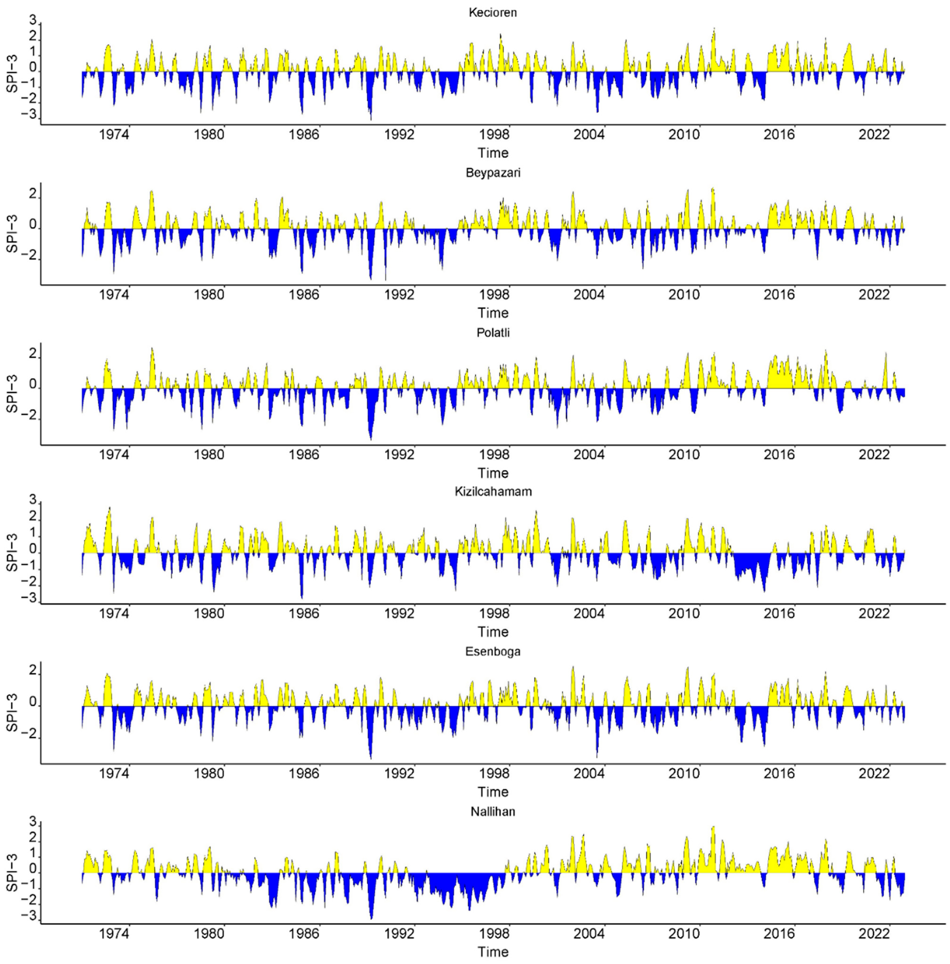
Figure 4 displays the time variation in the SPI-3 across many sites. In this figure, the climatic condition is divided into the two following categories: SPI-3 < 0 is a dry month and SPI-3 > 0 is a wet month. Figure 5 shows the temporal variation in dry months (SPI $<$ 0). It displays the overall number of droughts every year. The extreme and least drought events are observed at different stations. The total number of drought events over 52 years at each station is provided in Figure 6.

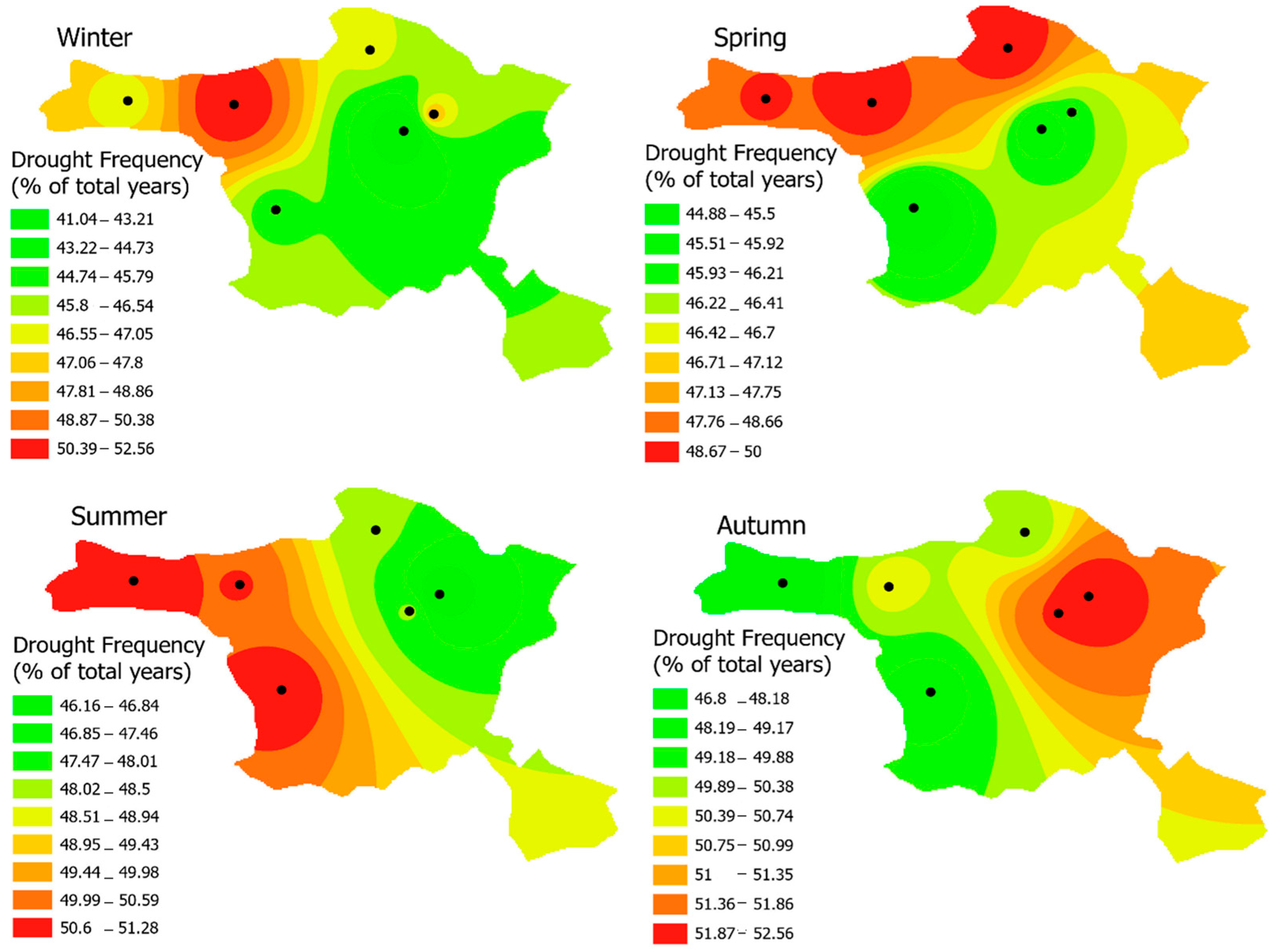
The well-known Inverse Distance Weighting approach was applied to calculate the drought counts in the non-selected area. In winter and spring, the drought counts are high in the northwest side of Ankara, while in the summer and fall season the drought counts are high in the southwest and east sides. To determine the seasonal frequency of drought events, the percentage of seasons with negative SPI-3 was calculated. Figure 7 illustrates how drought frequency varies by season. The drought frequency has a similar pattern to the drought counts. As suggested [31], the drought persistence at the seasonal scale was computed by dividing the frequency of drought events during two successive seasons by the total number of dry events (SPI-3 $\le$0) in the previous season.

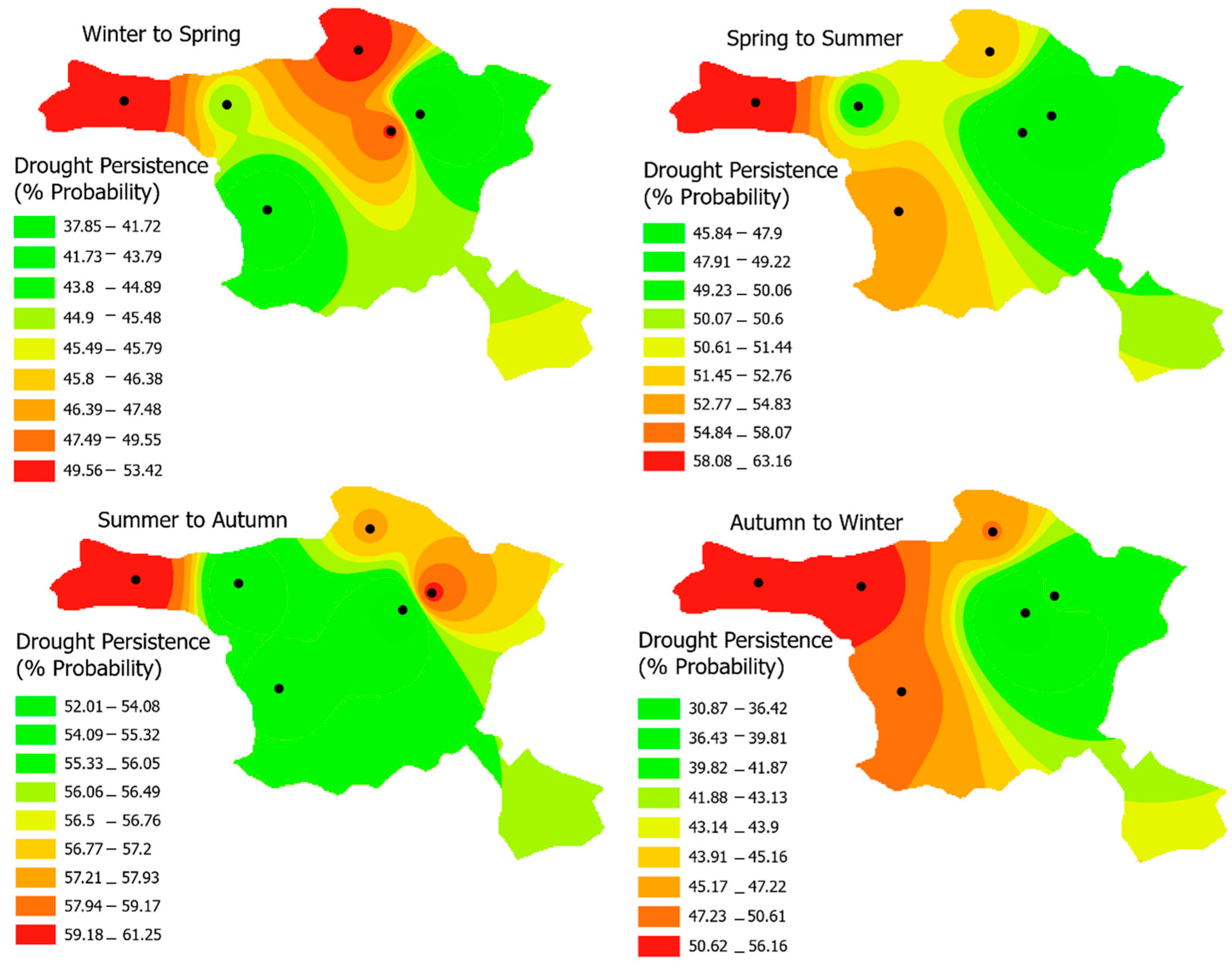
Figure 8 shows the chance of drought persistence. Droughts are more likely to persist over the summer–fall season. Moreover, BOPD models, including RELogRM and CFELogRM, are used to identify the significance of prior seasons on current seasons. The LR χ² and W χ² are applied to assess the significance of RELogRM and CFELogRM, the HT used to select the appropriate model for analyzing STIS drought persistence in the desired seasons.

Table 2. The test results for RELogRM and CFELogRM are shown, investigating fall-to-winter MD persistence. The results of the BOPD with panel data, RELogRM, and CFELogRM are presented. Both models demonstrate good fit, with the CFELogRM model (LogL = −387.1431) compared to the RELogRM model (LogL = −406.3683). The W χ² and LR χ² tests indicate significant differences between the models, with p-values of 0.0000. However, since both models are suitable, the HT will be employed to determine the most appropriate model for capturing the complex dynamics of drought persistence, considering the STIS patterns. Based on the HT results, we will recommend the most suitable model for further analysis.

RELogRM		CFELogRM
Test	Values	Test	Values
LogL	−406.3683	LogL	−387.1431
W χ2	138.6200	LR χ2	200.94
Prob > χ2	0.0000	Prob > χ2	0.0000

presents the results of various statistical tests for the RELogRM and the CFELogRM in analyzing fall-to-winter MD persistence. The tests reveal that both models have significant goodness of fit, with log likelihood (LogL) values of −406.3683 for RELogRM and −387.1431 for CFELogRM. The W χ² = 138.6200 and the LR χ² = 200.94 indicate that both models have a highly significant fit, with p-values of 0.0000 (Prob > χ²). These results suggest that both RELogRM and CFELogRM are effective in modeling fall-to-winter MD persistence, with the CFELogRM providing a slightly better fit based on the LogL and χ² values. The table exhibits the LogL values, LR χ², W χ², and p-values for both models, implying that both RELogRM and CFELogRM are statistically significant. However, the HT shows a p-value of 0.6593, underscoring that RELogRM is the more suitable model for investigating drought persistence during the fall-to-winter season. This finding focuses on the suitability of the random effects Logit regression model in capturing the intricate dynamics of drought persistence during this time.

Table 3. The results of the RELogRM provided for the fall-to-winter MD persistence. The table presents the estimated coefficients, standard errors (S.E.), and odds ratio (O.R.) for the variable.

Drought	O.R.	S.E.	Z	$\mathit{p}>\left|\mathit{Z}\right|$	95% Confidence
SPI-3	0.2416	0.0291	−11.77	0.00	0.1907	0.3061
constant	0.2044	0.0254	−12.77	0.00	0.1602	0.2608
Drought
SPI-3	−1.4204	0.1206	−11.77	0.00	−1.6568	−1.1839
constant	−1.5979	0.1243	−12.77	0.00	−1.8315	−1.3442
$\mathrm{Sigma}\_\mu$	0.7145	0.1321			0.3410	0.7937
$\rho$	0.1820	0.0130			0.1103	0.2367
$\mathrm{LR} \mathrm{test} \mathrm{of} \rho$ = 0: χ2 (01) = 61.71					Prob > χ2 = 0.0009

presents the coefficients of the RELogRM, which uncovers the relationships between the predictor variables and the likelihood of drought persistence. Notably, the coefficient of SPI (0.2416) indicates that an increase in SPI-3 values during the winter is associated with a decreased likelihood of drought in the subsequent spring season. This finding implies that SPI-3 values in winter have a substantial impact on drought persistence in spring. Furthermore, the proportion of variance elucidated by the panel-level variance factor is added by the coefficient ρ, which is calculated as ρ = δ²α/(δ²α + δ²γ), where δ²α represents the panel-level variance and δ²γ signifies the variation in γ (i.e., the error term). The error term γ is delivered with a mean of zero and a variance of π²/3. A value of ρ close to zero denotes the minimal importance of the panel-level variance component. For the winter-to-spring season, the determined value of ρ is 0.1820, indicating that the panel-level variance component accounts for approximately 18% of the total variance. In addition, the likelihood ratio test yields a value of 61.71 with a corresponding p-value of 0.009, suggesting that the effect of PD modeling is highly significant. This result validates the importance of accounting for PD formations in modeling drought persistence.

Table 4. The RELogRM and CFELogRM results attained for the winter-to-spring MD persistence.

RELogRM		CFELogRM
Test	Values	Test	Values
LogL	−360.5064	LogL	−343.2903
W χ2 (1)	166.4500	LR χ2 (1)	260.20
Prob > χ2	0.0000	Prob > χ2	0.0000

exhibits the scores of the statistical tests for RELogRM and CFELogRM, exploring the spatiotemporal persistence of drought from winter to spring. The outcomes include the log likelihood (LogL) values, and the LR χ², W χ², and p-values for both models, presenting a thorough assessment of their performance and significance. The HT yields a p-value of 0.8177, verifying the appropriateness of RELogRM for modeling the spatiotemporal dynamics of winter-to-spring drought persistence. This understanding underscores the weight of accounting for random effects in capturing the complicated relationships between the predictors and the likelihood of drought persistence during this season.

Table 5. The RELogRM results attained for the winter-to-spring MD persistence. The table presents the estimated coefficients, standard errors (S.E.), and odds ratio (O.R.) for the variable.

Drought	O.R.	S.E.	Z	$\mathit{p}>\left|\mathit{Z}\right|$	95% Confidence
SPI-3	0.2018	0.0250	−12.90	0.00	0.1583	0.2574
constant	0.2044	0.0254	−15.66	0.00	0.1347	0.2105
Drought
SPI-3	−1.6002	0.1240	−12.90	0.00	−1.8433	−1.3571
constant	−1.5979	0.1243	−15.66	0.00	−2.0043	−1.5583
$\mathrm{Sigma}\_\mu$	0.6732	0.1025			0.4137	0.7724
$\rho$	0.1253	0.0189			0.0876	0.1880
$\mathrm{LR} \mathrm{test} \mathrm{of} \rho$ = 0: χ2 (01) = 32.88					Prob > χ2 = 0.0049

provides the results of RELogRM for winter-to-spring spatiotemporal drought persistence modeling. The SPI-3 coefficient has the ratio of 0.2018 with a standard error of 0.0250, which suggests that the increase in SPI-3 values for winter declines the likelihood of a drought event in the spring season, while a decrease in SPI-3 for the winter season will increase the likelihood of a drought in the spring season. The $\rho =0.1253$, which is different from zero, and p value for $\rho$ is 0.0049, indicating that the panel level of variance is important and validating the use of PD model.

Table 6. RELOGRM and CFELOGRM results attained for the persistence of spring-to-summer MD.

RELogRM		CFELogRM
Test	Values	Test	Values
LogL	−393.0763	LogL	−374.8795
W χ2 (1)	165.0900	W χ2 (1)	262.31
Prob > χ2	0.0000	Prob > χ2	0.0000

shows the results for various tests in spring-to-summer season spatiotemporal drought persistence modeling. The LogL values, and the LR χ², W χ², and p values for the CFELogRM and RELogRM are given. The HT provides a p value of 0.6679, confirming that RELogRM is appropriate for spatiotemporal spring-to-summer drought persistence modeling.

Table 7. The results attained from the RELogRM are provided for the spring-to-summer MD persistence. The table presents the estimated coefficients, standard errors (S.E.), and odds ratio (O.R.) for the variable.

Drought	O.R.	S.E.	Z	$\mathit{p}>\left|\mathit{Z}\right|$	95% Confidence
SPI-3	0.2124	0.0256	−12.85	0.00	0.1678	0.2691
constant	0.2044	0.0254	−13.63	0.00	0.2173	0.2707
Drought	Coefficient	Std. error	Z	$\mathit{p}>\left|Z\right|$	[95% conf.	interval]
SPI-3	−1.5489	0.1205	−12.85	0.00	−1.7851	−1.3126
constant	−1.5261	0.1120	−13.63	0.00	−1.7455	−1.3066
$\mathrm{Sigma}\_\mu$	0.7808	0.1669			0.3932	0.9862
$\rho$	0.1519	0.0102			0.0756	0.1953
$\mathrm{LR} \mathrm{test} \mathrm{of} \rho$ = 0: χ2 (01) = 48.56					Prob > χ2 = 0.0051

provides the results of RELogRM for spring-to-summer spatiotemporal drought persistence modeling. The coefficient of SPI-3 has an odd ratio of 0.2124 with a standard error of 0.0256, which suggests that the increase in SPI-3 values for spring will reduce the occurrence probability of summer droughts, while a decrease in SPI-3 for spring will increase the likelihood of a drought in summer. The $\rho$ value is 0.1519, with a p value of 0.0051, which is again different from zero, suggesting that almost 15% of the variation is explained by the panel component and validating the use of PD modeling.

Table 8. The tests results of RELogRM and CFELogRM are given for the summer-to-fall MD persistence.

RELogRM		CFELogRM
Test	Values	Test	Values
LogL	−423.3450	LogLd	−407.5995
W χ2 (1)	169.4000	LR χ2 (1)	259.42
Prob > χ2	0.0000	Prob > χ2	0.0000

displays the findings obtained from several tests for summer-to-fall spatiotemporal drought persistence modeling. The LogL values, and the LR χ², W χ², and p values for the CFELogRM and RELogRM are provided. The HT returns a p value of 0.2367, supporting RELR’s suitability for spatiotemporal spring-to-summer drought persistence modeling.

Table 9. Results of the RELogRM for summer-to-fall MD persistence.

Drought	O.R.	S.E.	Z	$\mathit{p}>\left|\mathit{Z}\right|$	95% Confidence Interval
SPI-3	0.2180	0.0255	−13.02	0.00	0.1733	0.2742
constant	0.2730	0.0262	−13.49	0.00	0.2261	0.3297
SPI-3	−1.5230	0.1170	−13.02	0.00	−1.7524	−1.2937
constant	−1.5261	0.1120	−13.49	0.00	−1.4868	−1.1095
$\mathrm{Sigma}\_\mu$	0.6476	0.0688			0.4592	0.8424
$\rho$	0.1490	0.0302			0.0432	0.1798
LR test of ρ = 0: χ2 (01) = 48.12					Prob > χ2 = 0.0063

shows the results of RELogRM for summer-to-fall spatiotemporal drought persistence modeling. The coefficient of SPI-3 has an odd ratio of 0.2180 with a standard error of 0.0255, which shows that increasing the SPI-3 values for summer would lower the risk of drought occurrences in the fall season, while decreasing SPI-3 for the summer season will raise the possibility of drought in the fall season. The $\rho$ value of 0.1490, with a p-value of 0.0063, indicates that the panel component accounts for about 15% of the variance and supports the use of PD modeling.

5. Discussion

The historical precipitation data were utilized to classify drought occurrences. which were subsequently categorized into specific drought severity levels in Ankara. These classifications were determined using the SPI for a 3-month timescale that gives standardized values for precipitation at each station on a seasonal basis. Seasonal MD frequency and drought persistence are precarious factors in water resource management, agricultural productivity, energy consumption, and crop yield outcomes [38,39,40,41,42]. Despite their significance, there is a dearth of research in the literature centering on these aspects, particularly in the context of seasonal drought patterns. This gap underscores the need for dynamic and robust methodologies in drought monitoring, which are essential for delivering timely relief to drought-affected regions. The present study systematically investigated seasonal drought frequency and persistence over Ankara. In the relevant literature, several researchers applied logistic regression and random forest for monitoring drought persistence; however, these techniques do not capture the temporal aspects of the observed data. The proposed methodology is more suitable for the spatiotemporal analysis, and for the first time, the methods were applied for spatiotemporal monitoring of MD across Ankara. The outcomes of this analysis are anticipated to provide detailed insights into the SPI variation that affects the likelihood of drought in subsequent seasons. Therefore, feature early warning systems and mitigation strategies may use the findings to improve the forecasting accuracy of the evolved models. Seasonal drought monitoring has garnered significant attention from researchers, prompting numerous studies that aim to elucidate spatiotemporal drought patterns in a more robust manner. Traditional statistical approaches, such as linear regression, are limited to continuous dependent variables. Thus, categorical-based frameworks like logistic regression were suggested in this study [33,37]. Like the study conducted by Niaz et al. [37], we examined the frequency and duration of seasonal droughts utilizing SPI-3 and logistic regression modeling. Our findings agree with those of [37], in which logistic regression was found as an appropriate method to quantify the odds and probability of drought persistence across consecutive seasons. Given more attention to the models’ accuracy, our findings indicated the promising results of the advanced RELogRM and CFELogRM models used in the present study. In another study, Niaz et al. [34] have also proven the investigated the appropriateness of the RELogRM and CFELogRM techniques to identify spatiotemporal and intersessional characteristics. In the present study, the significance of RELogRM and CFELogRM was supported by the LR χ² and W χ², the novelty of which is warranted from the methodological perspectives.

To examine drought persistence in Ankara, we applied BOPD models across the dataset encompassing multiple stations. The statistical significance of these models was evaluated using LR χ² and W χ² tests. Outcomes demonstrate that both models are statistically robust for analyzing spatiotemporal drought persistence, with the HT indicating a preference for the RELogRM. For instance, in modeling winter-to-spring drought persistence, the HT produced a p-value of 0.8177, affirming the suitability of the RELogRM for capturing spatiotemporal dynamics in this context. In the winter-to-spring persistence model, the SPI-3 finding confirms that an increase in SPI-3 values during winter is associated with a reduced likelihood of drought occurrence in the subsequent spring, while a decrease in SPI-3 during winter elevates the probability of spring drought. The intraclass correlation coefficient indicates significant panel-level variance, thereby validating the application of a PD model. Similarly, the analysis of summer-to-fall drought persistence was assessed using LogL values, along with LR χ² and W χ² tests, supporting the RELogRM as the preferred model. The HT returned a p-value reinforcing the model’s appropriateness for this seasonal transition. The SPI-3 coefficient in this model indicates that higher SPI-3 values in summer are linked to a decreased risk of fall drought, whereas lower SPI-3 values increase the likelihood of drought in fall. The ρ value suggests the importance of using a PD model in this analysis.

Overall, the application of BOPD models has yielded critical insights into the spatiotemporal patterns of drought across Ankara, contributing to the advancement of scientific understanding and providing a foundation for more effective water resource management strategies. Furthermore, while this analysis focused solely on precipitation data, incorporating other climatological variables is crucial that can enhance modeling capabilities. Future research can explore Bayesian analysis and emerging machine learning approaches to detect inter-seasonal variation and model the relationships between variables and drought persistence, providing policymakers with informed decision-making tools. The scope of this study was limited to in situ observations across Ankara Province. Future studies could include remote climate data and satellite images, as suggested by Hayawi et al. [43], to consider additional geographic regions beyond Ankara, providing a more comparative analysis across different areas and addressing drought challenges on a broader spatial and temporal scales.

6. Conclusions

Water scarcity and water floods are serious problems in Turkey that need specific attention to mitigate their impacts on sustainable watershed development [44]. Effective drought management is essential for sustainable development in the country [24]. In this study, we employed BOPD models, RELogRM and CFELogRM, to investigate drought persistence across capital province of Turkey. The significance of these models was evaluated using the LR χ² and W χ², tests. Our results indicated that both models are statistically significant for monitoring spatiotemporal drought persistence, but the HT confirms that RELogRM is the more appropriate specification. For example, for winter to spring, the HT gives a p-value of 0.8177, confirming that RELogRM is appropriate for spatiotemporal winter-to-spring drought persistence modeling. The coefficient of SPI-3 has an odd ratio of 0.2018 with a standard error of 0.0250, which suggests that the increase in SPI-3 values for winter will decrease the likelihood drought occurrences in the spring season, while a decrease in SPI-3 for the winter season will increase the likelihood of drought in the spring season. The ρ = 0.1253, which is different from zero, and the p-value for ρ is 0.0049, indicating that the panel level of variance is important and validating the use of the PD model. Similarly, summer-to-fall spatiotemporal drought persistence modeling is assessed by the LogL, LR χ² and W χ², and p values for the CFELogRM and RELogRM. The HT returns a p value of 0.2367, supporting RELR’‘s suitability for spatiotemporal spring-to-summer drought persistence modeling. The coefficient of SPI-3 has an odd ratio of 0.2180 with a standard error of 0.0255, which shows that increasing SPI-3 values for summer would lower the risk of drought occurrences in the fall season, while decreasing SPI-3 for the summer season will raise the possibility of drought in the fall season. The ρ value of 0.1490, with a p-value of 0.0063, indicates that the panel component accounts for about 15% of the variance and supports the use of PD modeling.