
Ecosystem Services’ Supply–Demand Assessment and Ecological Management Zoning in Northwest China: A Perspective of the Water–Food–Ecology Nexus

Abstract
1. Introduction
2. Materials and Methods
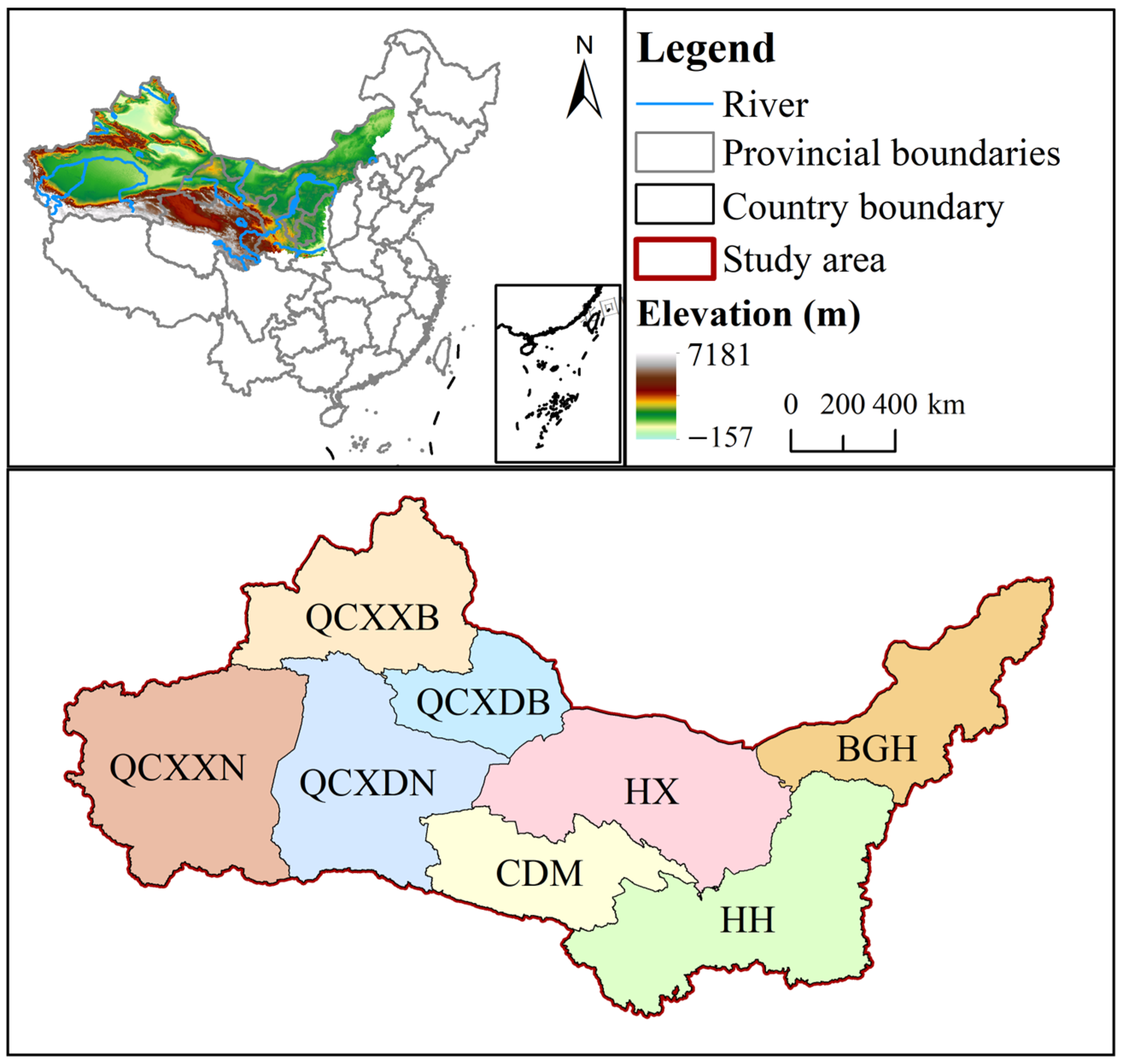
2.1. Study Area
2.2. Data Sources
2.3. Research Framework
2.4. Methods
2.4.1. Quantification of ESSD
- (1)
- FP
- (2)
- WY
- (3)
- CS
2.4.2. Trade-Offs and Synergy Analysis of ESs
- (1)
- Temporal trade-off and synergy analysis
- (2)
- Spatial trade-off and synergy analysis
2.4.3. Matching Evaluation of ESSD
- (1)
- Quantity matching
- (2)
- Spatial matching
- (3)
- Risk identification
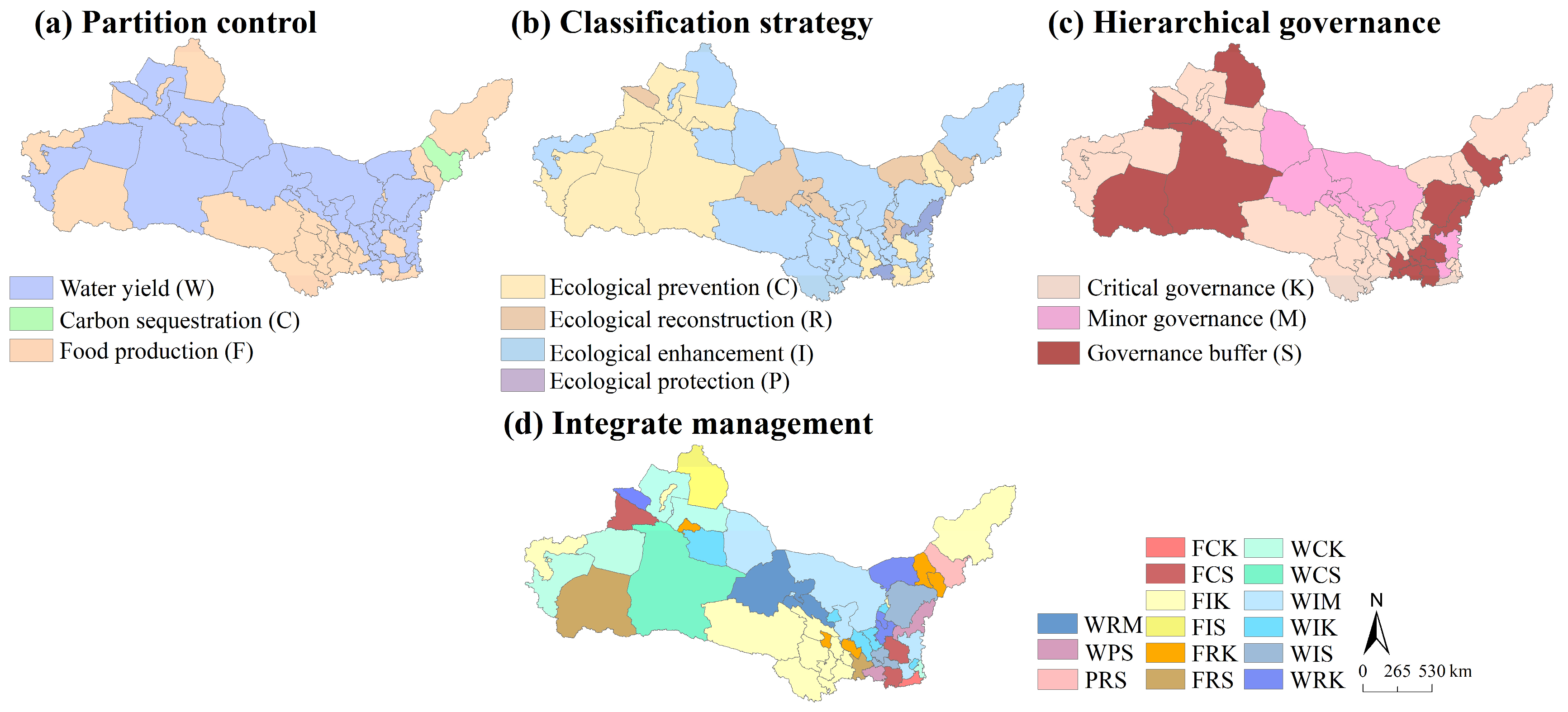
2.4.4. Ecological Management Zoning Method
3. Result
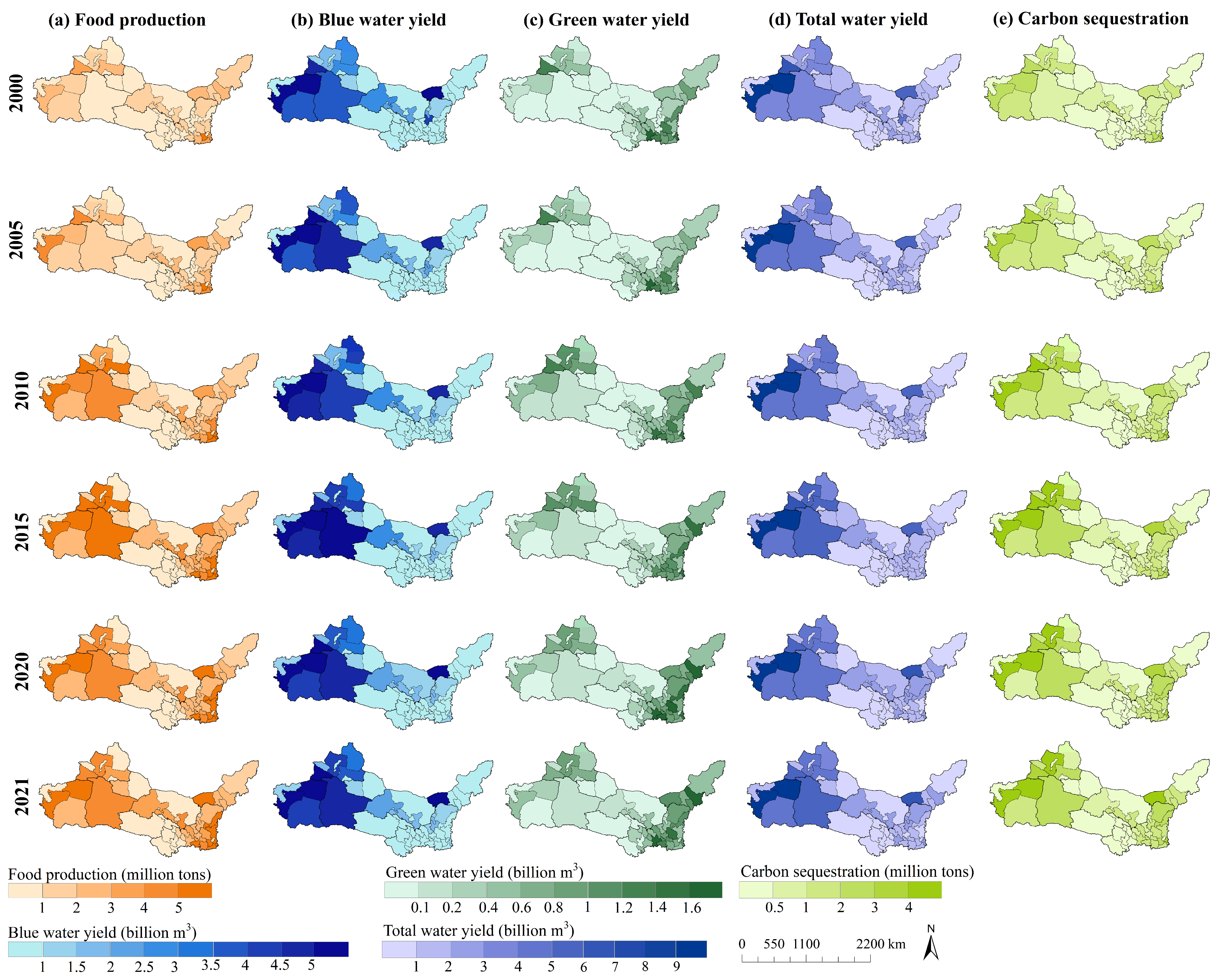
3.1. Spatiotemporal Evolution of ESSD
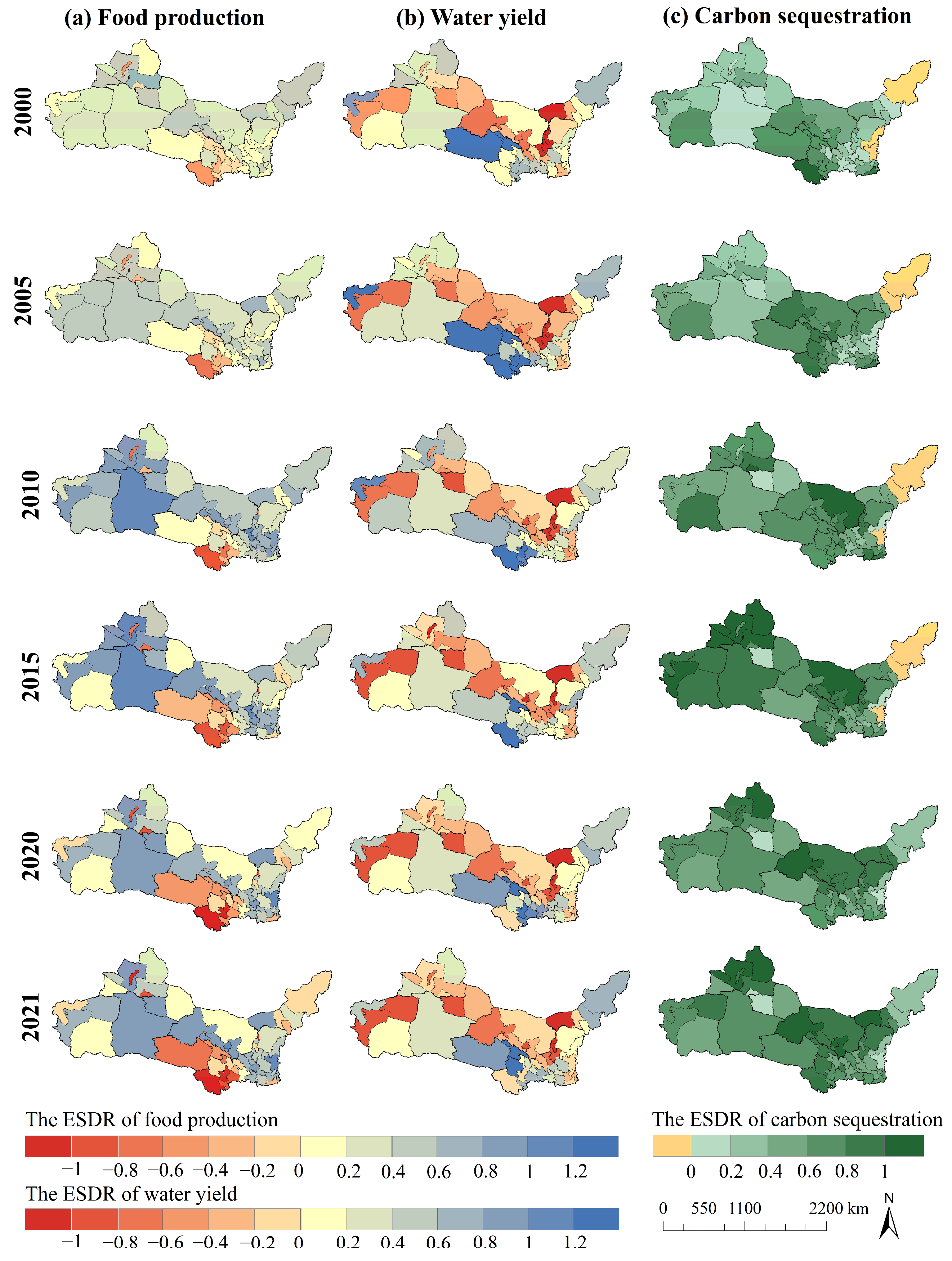
3.1.1. Ess’ Supply
- (1)
- FP
- (2)
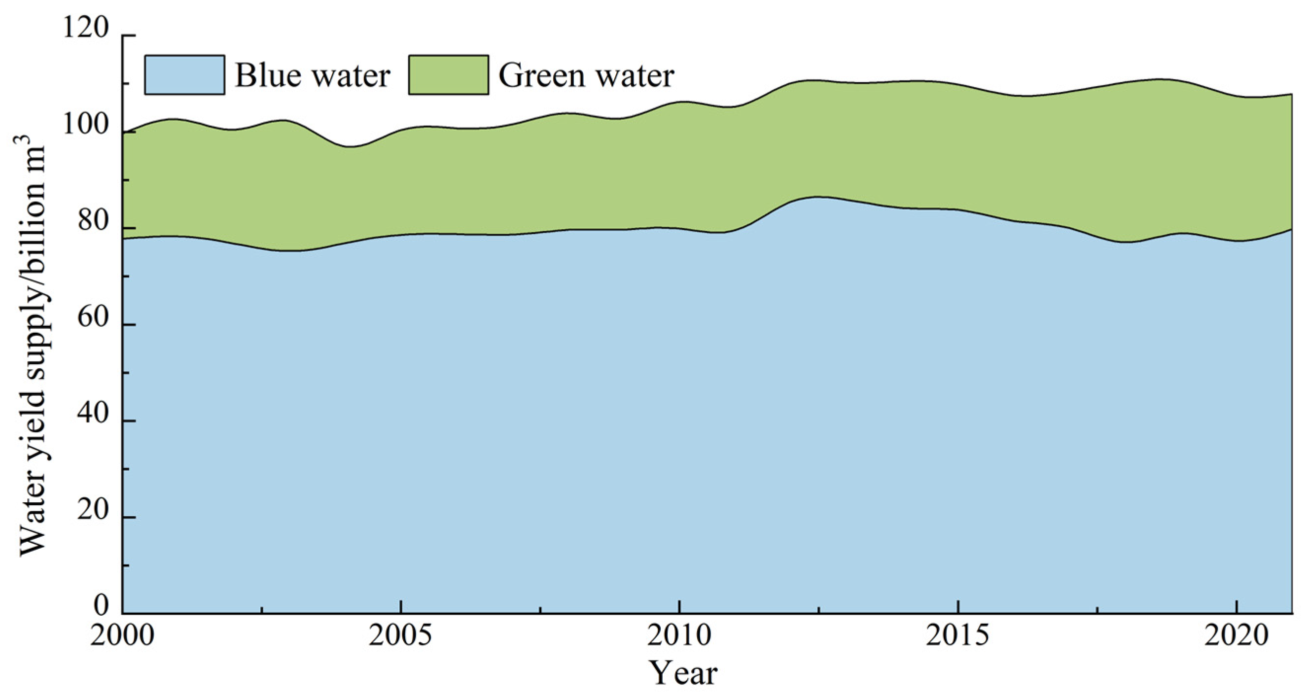
- WY
- (3)
- CS
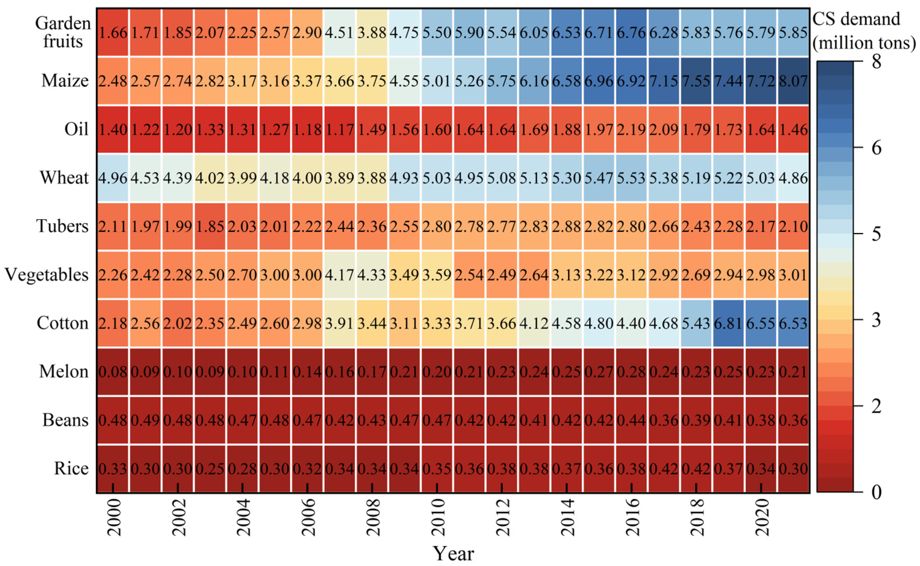
3.1.2. Ess’ Demand
- (1)
- FP
- (2)
- WY
- (3)
- CS
3.2. Trade-Offs and Synergies of ESs
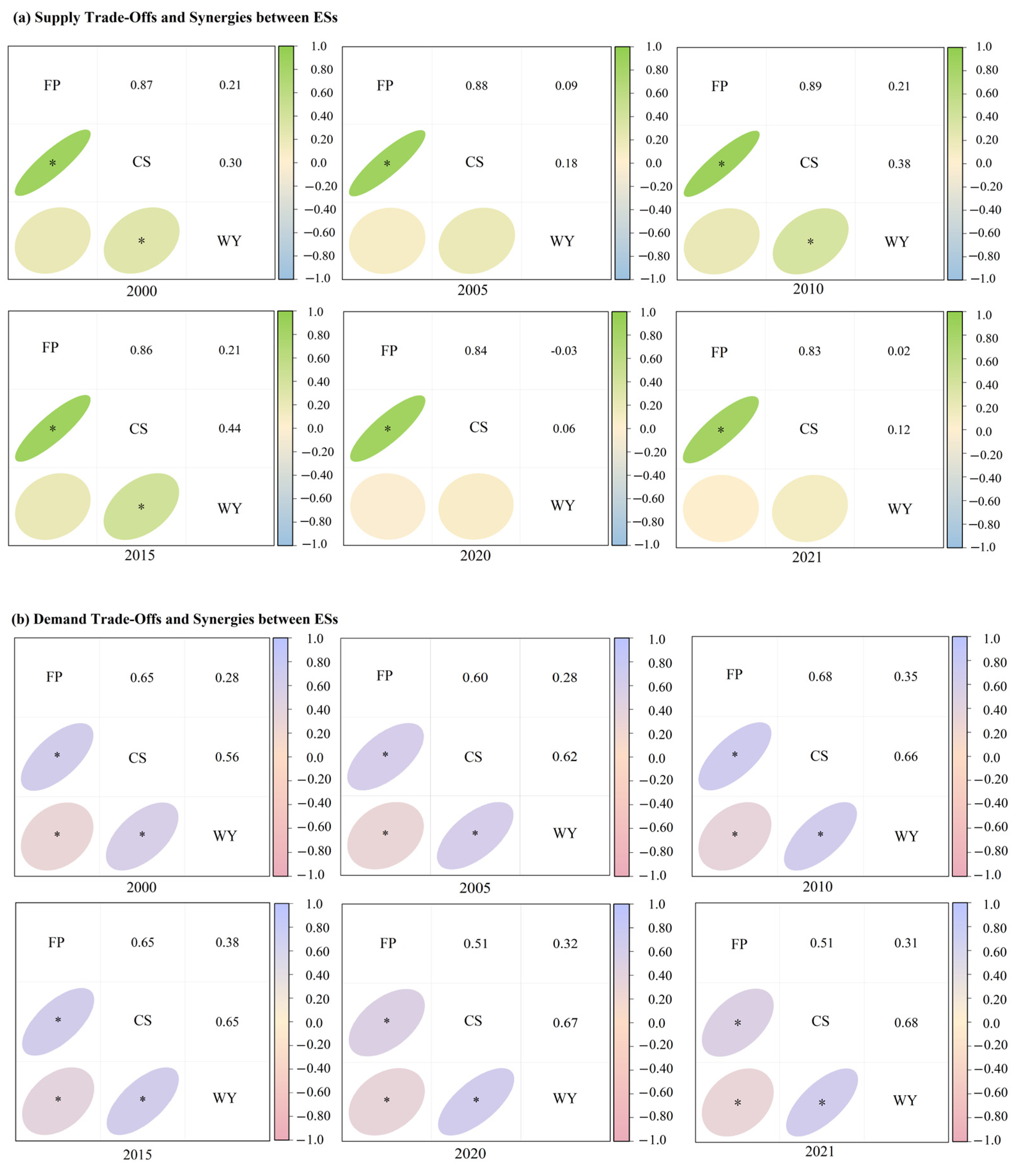
3.2.1. Supply Trade-Offs and Synergies between ESs
3.2.2. Demand Trade-Offs and Synergies between ESs
3.3. Supply–Demand Matching Characteristics of ESs
3.3.1. Quantity Matching
3.3.2. Spatial Matching
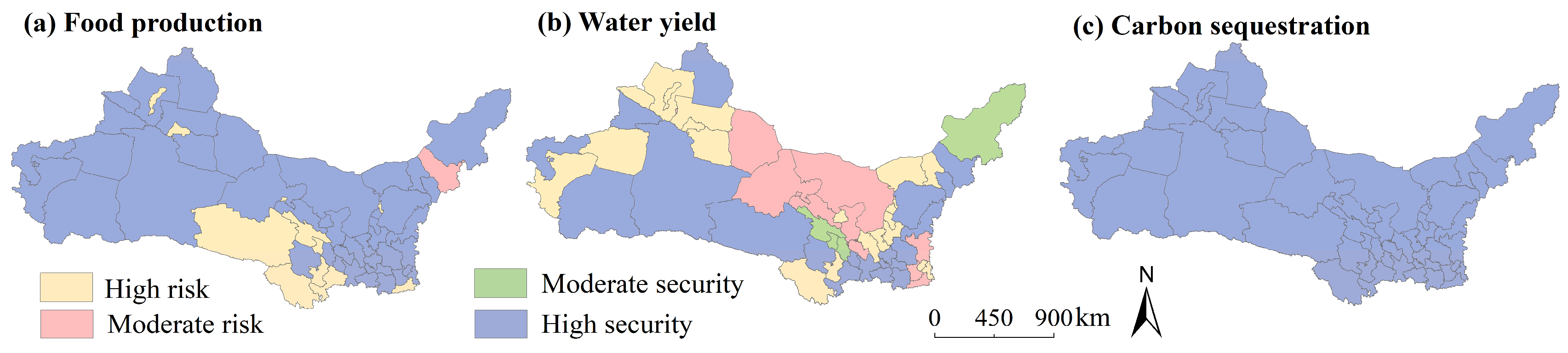
3.3.3. Risk Identification
3.4. Ecological Management Zoning
4. Discussion
4.1. Improved Approach to Assessing Ecosystem Services’ Supply and Demand
4.2. Rationality of Ecological Management Zoning
4.3. Governance Strategies for Diverse Zones
5. Conclusions
- (1)
- Throughout the research period, except for the inverted U-shaped change in demand for GWY and the supply for BWY, all other ESSDs significantly increased. Maize, wheat, cotton, vegetables, and garden fruits had a higher demand for ESs. Spatially, the supply and demand of ESs exhibited significant heterogeneity, with most showing a pattern of “high in the west and low in the middle”.
- (2)
- All three ESs exhibited a synergistic relationship. But over time, the synergistic effect weakened. Spatially, the strong synergistic relationship between FP supply and WY supply, FP supply and CS supply, and WY supply and CS supply was mainly distributed in Xinjiang, HH, and BGH. Meanwhile, the synergistic relationship between ESs’ demands all presented the spatial pattern of “high in the east and low in the west”.
- (3)
- The ESDR for FP and CS in WTL increased, while the ESDR for WY decreased, and the supply was smaller than the demand. Spatially, the distribution pattern of the ESDR for FP and WY was the opposite. CS showed a supply and demand surplus in most cities. The FP and CS were dominated by the low supply–low demand space match, whereas the WY was dominated by the high supply–high demand space match. Further, FP was the highest risk in CDM, and WY was the highest risk in HX, HH, and both sides of the “Qice line”, while CS was highly safe in all cities.
- (4)
- Based on the features and matching patterns of ESSD, a spatial management framework was constructed to delineate ecosystem management zones and provide suggestions for different zones. Meanwhile, the proposed framework and adopted indicators offer new insights into understanding ecological governance under the WFE nexus.
Author Contributions
Funding
Data Availability Statement
Conflicts of Interest
References
- Burkhard, B.; Kroll, F.; Nedkov, S.; Müller, F. Mapping ecosystem service supply, demand and budgets. Ecol. Indic. 2012, 21, 17–29. [Google Scholar] [CrossRef]
- Ding, T.H.; Chen, J.F.; Fang, L.P.; Ji, J.; Fang, Z. Urban ecosystem services supply-demand assessment from the perspective of the water-energy-food nexus. Sustain. Cities Soc. 2023, 90, 104401. [Google Scholar] [CrossRef]
- Hasan, S.S.; Zhen, L.; Miah, M.G.; Ahamed, A.; Samie, A. Impact of land use change on ecosystem services: A review. Environ. Dev. 2020, 34, 100527. [Google Scholar] [CrossRef]
- Fu, B.J.; Wei, Y.P. Editorial overview: Keeping fit in the dynamics of coupled natural and human systems. Curr. Opin. Environ. Sustain. 2018, 33, A1–A4. [Google Scholar] [CrossRef]
- Yuan, Y.; Bai, Z.K.; Zhang, J.J.; Huang, Y.H. Investigating the trade-offs between the supply and demand for ecosystem services for regional spatial management. J. Environ. Manag. 2023, 325, 116591. [Google Scholar] [CrossRef]
- Zhang, J.X.; Deng, M.J.; Han, Y.P.; Huang, H.P.; Yang, T. Spatiotemporal variation of irrigation water requirements for grain crops under climate change in Northwest China. Environ. Sci. Pollut. Res. 2023, 30, 45711–45724. [Google Scholar] [CrossRef] [PubMed]
- Deng, M.J. “Three Water Lines” strategy: Its spatial patterns and effects on water resources allocation in Northwest China. J. Geogr. Sci. 2018, 73, 1189–1203. (In Chinese) [Google Scholar] [CrossRef]
- Zhao, Y.; Huang, K.J.; Gao, X.R.; An, T.L.; He, G.H.; Jiang, S. Evaluation of grain production water footprint and influence of grain virtual water flow in the Yellow River Basin. Water Resour. Prot. 2022, 38, 39–47. [Google Scholar] [CrossRef]
- Yin, D.Y.; Yu, H.C.; Shi, Y.Y.; Zhao, M.Y.; Zhang, J.; Li, X.S. Matching supply and demand for ecosystem services in the Yellow River Basin, China: A perspective of the water-energy-food nexus. J. Clean. Prod. 2023, 384, 135469. [Google Scholar] [CrossRef]
- Liu, Y.; Bi, J.; Lv, J.S.; Wang, C. Spatial multi-scale relationships of ecosystem services: A case study using a geostatistical methodology. Sci. Rep. 2017, 7, 9486. [Google Scholar] [CrossRef]
- Teng, Y.M.; Chen, G.D.; Su, M.R.; Zhang, Y.; Li, S.T.; Xu, C. Ecological management zoning based on static and dynamic matching characteristics of ecosystem services supply and demand in the Guangdong-Hong Kong-Macao Greater Bay Area. J. Clean. Prod. 2024, 448, 141599. [Google Scholar] [CrossRef]
- You, C.; Qu, H.J.; Wang, C.B.; Feng, C.C.; Guo, L. Trade-off and synergistic of ecosystem services supply and demand based on socio-ecological system (SES) in typical hilly regions of south China. Ecol. Indicat. 2024, 160, 111749. [Google Scholar] [CrossRef]
- Talukdar, S.; Singha, P.; Shahfahad; Mahato, S.; Praveenk, B. Dynamics of ecosystem services (ESs) in response to land use land cover (LU/LC) changes in the lower Gangetic plain of India. Ecol. Indicat. 2020, 112, 106121. [Google Scholar] [CrossRef]
- Feng, Q.; Zhao, W.W.; Hu, X.P.; Liu, Y.; Daryanto, S.; Cherubini, F. Trading-off ecosystem services for better ecological restoration: A case study in the Loess Plateau of China. J. Clean. Prod. 2020, 257, 120469. [Google Scholar] [CrossRef]
- Benra, F.; Frutos, A.D.; Gaglio, M.; Garretón, C.A.; Lucia, M.F.; Bonn, A. Mapping water ecosystem services: Evaluating InVEST model predictions in data scarce regions. Environ. Model. Softw. 2021, 138, 104982. [Google Scholar] [CrossRef]
- Chen, Y.M.; Zhai, Y.P.; Gao, J.X. Spatial patterns in ecosystem services supply and demand in the Jing-Jin-Ji region, China. J. Clean. Prod. 2022, 361, 132177. [Google Scholar] [CrossRef]
- Zhang, Z.M.; Peng, J.; Xu, Z.H.; Wang, X.Y.; Meersmans, J. Ecosystem services supply and demand response to urbanization: A case study of the Pearl River Delta, China. Ecosyst. Serv. 2021, 49, 101274. [Google Scholar] [CrossRef]
- Xin, R.H.; Skov-Petersena, H.; Zeng, J.; Zhou, J.H.; Li, K.; Hu, J.Q.; Liu, X.; Kong, J.W.; Wang, Q.W. Identifying key areas of imbalanced supply and demand of ecosystem services at the urban agglomeration scale: A case study of the Fujian Delta in China. Sci. Total Environ. 2021, 791, 148173. [Google Scholar] [CrossRef]
- Wu, J.S.; Fan, X.N.; Li, K.Y.; Wu, Y.W. Assessment of ecosystem service flow and optimization of spatial pattern of supply and demand matching in Pearl River Delta, China. Ecol. Indic. 2023, 153, 110452. [Google Scholar] [CrossRef]
- Zeng, X.T.; Zhang, Z.M.; Wang, J.X.; Zhao, Y.L. Analysis and Prospect of China’s Food Consumption. Agric. Outlook. 2021, 17, 104–114. (In Chinese) [Google Scholar]
- Yuan, M.; Lo, S. Ecosystem services and sustainable development: Perspectives from the food-energy-water Nexus. Ecosyst. Serv. 2020, 46, 101217. [Google Scholar] [CrossRef]
- Zhu, Y.H.; Hou, Z.D.; Xu, C.X.; Gong, J. Ecological risk identification and management based on ecosystem service supply and demand relationship in the Bailongjiang River Watershed of Gansu Province. Sci. Geogr. Sinica. 2023, 43, 423–433. (In Chinese) [Google Scholar] [CrossRef]
- Ding, Q.; Wang, L.; Fu, M.C. Spatial characteristics and trade-offs of ecosystem services in arid central Asia. Ecol. Indic. 2024, 161, 111935. [Google Scholar] [CrossRef]
- Sun, R.; Jin, X.; Han, B.; Liang, X.; Zhang, X.; Zhou, Y. Does scale matter? Analysis and measurement of ecosystem service supply and demand status based on ecological unit. Environ. Impact Assess. Rev. 2022, 95, 106785. [Google Scholar] [CrossRef]
- Zhang, J.X.; Yang, T.; Deng, M.J.; Huang, H.P.; Han, Y.P.; Xu, H.H. Spatiotemporal variations and its driving factors of NDVI in Northwest China during 2000–2021. Environ. Sci. Pollut. Res. 2023, 30, 118782–118800. [Google Scholar] [CrossRef] [PubMed]
- Zhang, J.X.; Deng, M.J.; Li, P.; Li, Z.B.; Huang, H.P.; Shi, P.; Feng, C.H. Security Pattern and Regulation of Agricultural Water Resources in Northwest China from the Perspective of Virtual Water Flow. Engineering 2022, 24, 14. [Google Scholar] [CrossRef]
- Shangguan, C.X.; Lu, Y.; Jing, L.; Du, T.; Sun, J.J.; Zhang, X.Y. Supply-Demand Forecast and Structure Adjustment Paths of Planting and Breeding Industries Based on Changes in Food Consumption. Strateg. Study CAE 2023, 25, 128–136. [Google Scholar] [CrossRef]
- Liu, L.C.; Hu, X.T.; Zhan, Y.J.; Sun, Z.X.; Zhang, Q. China’s dietary changes would increase agricultural blue and green water footprint. Sci. Total Environ. 2023, 903, 165763. [Google Scholar] [CrossRef]
- Fridman, D.; Biran, N.; Kissinger, M. Beyond blue: An extended framework of blue water footprint accounting. Sci. Total Environ. 2021, 777, 146010. [Google Scholar] [CrossRef]
- Li, X.Y.; Zou, L.; Xia, J.; Zhang, L.P.; Wang, F.Y.; Li, M.X. Response of blue-green water to climate and vegetation changes in the water source region of China’s South-North water Diversion Project. J. Hydrol. 2024, 634, 131061. [Google Scholar] [CrossRef]
- Falkenmark, M. Land and Water Integration and River Basin Management; Food and Agriculture Organization of the United Nations: Rome, Italy, 1995. [Google Scholar]
- Hunink, J.E.; Droogers, P.; Kauffman, S.; Mwaniki, B.M.; Bouma, J. Quantitative simulation tools to analyze up and downstream interactions of soil and water conservation measures: Supporting policy making in the green water credits program of Kenya. J. Environ. Manag. 2012, 111, 187–194. [Google Scholar] [CrossRef] [PubMed]
- Rockström, J.; Falkenmark, M. Agriculture: Increase water harvesting in Africa. Nature 2015, 519, 283–285. [Google Scholar] [CrossRef]
- Wu, F.; Yang, X.L.; Cui, Z.Y.; Ren, L.L.; Jiang, S.H.; Liu, Y.; Yuan, S.S. The impact of human activities on blue-green water resources and quantification of water resource scarcity in the Yangtze River Basin. Sci. Total Environ. 2024, 909, 168550. [Google Scholar] [CrossRef]
- Yang, J.; Xie, B.; Zhang, D.; Tao, W. Climate and land use change impacts on water yield ecosystem service in the Yellow River Basin, China. Environ. Earth Sci. 2021, 80, 72. [Google Scholar] [CrossRef]
- Zhao, S.X.; Wang, W.; Liu, Y.L.; Zhang, P.; Zhang, H.M. Spatiotemporal Evolution in Agricultural Water Stress in Sichuan Province Evaluated from the Perspective of Virtual Water. J. Irrig. Drain. 2023, 42, 85–90+121. (In Chinese) [Google Scholar] [CrossRef]
- Nie, Y.; Li, X.Y.; Jiang, W.Q.; Liu, N.J. Planting structure optimization of three main grain crops in 10 northern China provinces based on water footprint method. Resour. Sci. 2022, 44, 2315–2329. [Google Scholar] [CrossRef]
- Hoekstra, A.Y.; Hung, P.Q. Virtual Water Trade: A Quantification of Virtual Water Flows between Nations in Relation to International Crop Trade; Value of Water Research Report Series No.11; UNESCO-IHE Institute for Water Education: Delft, The Netherlands, 2002. [Google Scholar]
- Hoekstra, A.Y.; Chapagain, A.K.; Mekonnen, M.M.; Aldaya, M.M. The Water Footprint Assessment Manual: Setting the Global Standard; Routledge: London, UK, 2011. [Google Scholar] [CrossRef]
- Liu, X.; Xu, Y.; Sun, S.; Zhao, X.; Wang, Y. Analysis of the Coupling Characteristics of Water Resources and Food Security: The Case of Northwest China. Agriculture 2022, 12, 1114. [Google Scholar] [CrossRef]
- Sun, S.K.; Yin, Y.L.; Wu, P.T.; Wang, Y.B.; Luan, X.B.; Li, C. Geographical Evolution of Agricultural Production in China and Its Effects on Water Stress, Economy and the Environment: The Virtual Water Perspective. Water Resour. Res. 2019, 55, 4014–4029. [Google Scholar] [CrossRef]
- Yang, X.; Bai, B.; Bai, Z. Research on Spatiotemporal Changes in Carbon Footprint and Vegetation Carbon Carrying Capacity in Shanxi Province. Forests 2023, 14, 1295. [Google Scholar] [CrossRef]
- Cui, Y. Study on the Coordination of China’s Agricultural Carbon Footprint and Economic Development—Analysis Based on the Carbon Sink Effect; Northwest A&F University: Xianyang, China, 2022. (In Chinese) [Google Scholar]
- Ning, X.S. Study on the General Situation of Planting Industry, Temporal and Spatial Evolution Characteristics of Carbon Emission and Emission Reduction Potential in Three Provinces of Northeast China; Agricultural College, Northeast Agricultural University: Harbin, China, 2023. (In Chinese) [Google Scholar]
- Nayak, A.K.; Tripathi, R.; Debnath, M.; Swain, C.K.; Dhal, B.; Vijaykumar, S.; Nayak, A.D.; Mohanty, S.; Shahid, M.; Kumar, A.; et al. Carbon and water footprints of major crop production in India. Pedosphere 2023, 33, 448–462. [Google Scholar] [CrossRef]
- Yu, J.W. Research on Water-Crop-Energy-Ecosystem Nexus in the Yarkant River Basin; Shihezi University: Shihezi, China, 2022. (In Chinese) [Google Scholar]
- Yang, L.; Han, Q.; Bauke, D.V. Urbanization effects on the food-water-energy nexus within ecosystem services: A case study of the Beijing-Tianjin-Hebei urban agglomeration in China. Ecol. Indic. 2024, 160, 111845. [Google Scholar] [CrossRef]
- Luo, Y.; Yang, D.W.; O’Connor, P.; Wu, T.H.; Ma, W.J.; Xu, L.L.; Guo, R.F.; Lin, J.Y. Dynamic characteristics and synergistic effects of ecosystem services under climate change scenarios on the Qinghai–Tibet Plateau. Sci. Rep. 2022, 12, 2540. [Google Scholar] [CrossRef]
- Li, W.; Geng, J.; Bao, J.; Lin, W.; Wu, Z.; Fan, S. Analysis of Spatial and Temporal Variations in Ecosystem Service Functions and Drivers in Anxi County Based on the InVEST Model. Sustainability 2023, 15, 10153. [Google Scholar] [CrossRef]
- Xiu, Y.; Wang, N.; Peng, F.; Wang, Q. Spatial–Temporal Variations of Water Ecosystem Services Value and Its Influencing Factors: A Case in Typical Regions of the Central Loess Plateau. Sustainability 2022, 14, 7169. [Google Scholar] [CrossRef]
- Tan, F.; Lu, Z.; Zeng, F. Study on the trade-off/synergy spatiotemporal benefits of ecosystem services and its influencing factors in hilly areas of southern China. Front. Ecol. Evol. 2024, 11, 1342766. [Google Scholar] [CrossRef]
- Cui, F.; Tang, H.; Zhang, Q.; Wang, B.; Dai, L. Integrating ecosystem services supply and demand into optimized management at different scales: A case study in Hulunbuir, China. Ecosyst. Serv. 2019, 39, 100984. [Google Scholar] [CrossRef]
- González-García, A.; Palomo, I.; González, J.A.; López, C.A.; Montes, C. Quantifying spatial supply-demand mismatches in ecosystem services provides insights for land-use planning. Land. Use Pol. 2020, 94, 104493. [Google Scholar] [CrossRef]
- Zhao, X.; Ma, P.; Li, W.; Du, Y. Spatiotemporal changes of supply and demand relationships of ecosystem services in the Loess Plateau. Acta Geograph. Sin. 2021, 76, 2780–2796. [Google Scholar] [CrossRef]
- Li, K.; Hou, Y.; Andersen, P.S.; Xin, R.; Rong, Y.; Skov-Petersen, H. An ecological perspective for understanding regional integration based on ecosystem service budgets, bundles, and flows: A case study of the Jinan metropolitan area in China. J. Environ. Manag. 2022, 305, 114371. [Google Scholar] [CrossRef]
- Cao, X.C.; Shu, R.; Guo, X.P.; Shao, G.C.; Wang, Z.C. Water stresses evaluation of agricultural production in Jiangsu Province using BWSI and GWSI. Resour. Environ. Yangtze Basin 2017, 26, 856–864. (In Chinese) [Google Scholar] [CrossRef]
- Cheng, K.; Yan, M.; Nayak, D.; Pan, G.X.; Smith, P.; Zheng, J.F.; Zheng, J.W. Carbon footprint of crop production in China: An analysis of National Statistics data. J. Agric. Sci. 2015, 153, 422–431. [Google Scholar] [CrossRef]
- Song, J.; Liu, Y.Z.; Zhuang, M.H.; Gu, W.Y. Estimating crop carbon footprint and associated uncertainty at prefecture-level city scale in China. Resour. Conserv. Recycl. 2023, 199, 107263. [Google Scholar] [CrossRef]
- Schirpke, U.; Candiago, S.; Vigl, L.E. Integrating supply, flow and demand to enhance the understanding of interactions among multiple ecosystem services. Sci. Total Environ. 2019, 651, 928–941. [Google Scholar] [CrossRef]
- Yu, H.J.; Wei, X.; Sun, L.; Wang, Y.T. Identifying the regional disparities of ecosystem services from a supply-demand perspective. Resour. Conserv. Recycl. 2021, 169, 105557. [Google Scholar] [CrossRef]
- Xiang, H.X.; Zhang, J.; Mao, D.H.; Wang, Z.M.; Qiu, Z.Q.; Yan, H.Q. Identifying spatial similarities and mismatches between supply and demand of ecosystem services for sustainable Northeast China. Ecol. Indic. 2022, 134, 108501. [Google Scholar] [CrossRef]
- Zhai, T.L.; Zhang, D.; Zhao, C.C. How to optimize ecological compensation to alleviate environmental injustice in different cities in the Yellow River Basin? A case of integrating ecosystem service supply, demand and flow. Sustain. Cities Soc. 2021, 75, 103341. [Google Scholar] [CrossRef]
- Xu, Z.H.; Peng, J.; Dong, J.Q.; Liu, Y.X.; Liu, Q.Y.; Lyu, D.; Qian, R.L.; Zhang, Z. Spatial correlation between the changes of ecosystem service supply and demand: An ecological zoning approach. Landsc. Urban Plan. 2022, 217, 104258. [Google Scholar] [CrossRef]
- Wu, J.; Huang, Y.; Jiang, W. Spatial matching and value transfer assessment of ecosystem services supply and demand in urban agglomerations: A case study of the Guangdong-Hong Kong-Macao Greater Bay Area in China. J. Clean. Prod. 2022, 375, 134081. [Google Scholar] [CrossRef]
- Tian, J.; Zeng, S.; Zeng, J.; Jiang, F. Assessment of supply and demand of regional flood regulation ecosystem services and zoning management in response to flood disasters: A case study of Fujian delta. Int. J. Environ. Res. Public Health 2023, 20, 589. [Google Scholar] [CrossRef]
- Xin, C.H.; Guo, F.Q. Quantitative simulation of ecological compensation approaches in transboundary watersheds of China: A scenario analysis based on a multi-regional CGE model. Ecol. Indic. 2023, 155, 111048. [Google Scholar] [CrossRef]
- Tang, X.Y.; Huang, Y.; Pan, X.H.; Liu, T.; Ling, Y.N.; Peng, J.B. Managing the water-agriculture-environment-energy nexus: Trade-offs and synergies in an arid area of Northwest China. Agric. Water Manag. 2024, 295, 108776. [Google Scholar] [CrossRef]


| Data Types | Type and Resolution | Period | Database Sources |
|---|---|---|---|
| Soil | Raster, 1 km | - | Resource and Environment Science and Data Center http://www.resdc.cn/ |
| Land use | Raster, 30 m | 2000, 2005, 2010, 2015, 2020 | |
| DEM | Raster, 30 m | - | |
| Effective irrigation area | Statistical data | 2000~2021 | Water resource bulletins of provinces http://slt.shaanxi.gov.cn/ https://slt.gansu.gov.cn/ https://slt.nmg.gov.cn/ http://slt.nx.gov.cn/ https://slt.xinjiang.gov.cn/ http://slt.qinghai.gov.cn/ |
| Irrigation quota | 2000~2021 | ||
| Water consumption | 2000~2021 | ||
| Precipitation | Raster, 1 km | 2000~2021 | National Tibetan Plateau Scientific Data Center https://data.tpdc.ac.cn/ |
| Potential evapotranspiration | Raster, 1 km | 2000~2021 | |
| Crop production | Statistical data | 2000~2021 | China Rural Statistical Yearbook and Statistical Yearbooks of provinces https://www.stats.gov.cn/ http://tjj.shaanxi.gov.cn/ http://tjj.gansu.gov.cn/ http://tj.nmg.gov.cn/ http://tj.nx.gov.cn/ http://tjj.xinjiang.gov.cn/ http://tjj.qinghai.gov.cn/ |
| Crop area | 2000~2021 | ||
| Population | 2000~2021 | ||
| Population density | 2000~2021 | ||
| Per capita food consumption | 2000~2021 | ||
| Carbon emission factor | Statistical data | - | China Products Carbon Footprint Database http://lca.cityghg.com/ the China Emission Accounts and Datasets |
| Crop coefficient | Statistical data | - | [6] |
| Crop | Ci | Wc | Ef |
|---|---|---|---|
| rice | 0.41 | 0.12 | 0.45 |
| wheat | 0.49 | 0.12 | 0.4 |
| maize | 0.47 | 0.13 | 0.4 |
| bean | 0.45 | 0.13 | 0.34 |
| potato | 0.42 | 0.7 | 0.7 |
| oil | 0.45 | 0.1 | 0.25 |
| cotton | 0.45 | 0.08 | 0.1 |
| vegetable | 0.45 | 0.9 | 0.6 |
| garden fruit | 0.45 | 0.9 | 0.7 |
| melon | 0.45 | 0.9 | 0.7 |
| Element | Carbon Emission Factor | Element | Carbon Emission Factor | ||
|---|---|---|---|---|---|
| Seed | wheat | 0.66 kgCO2/kg | Fertilizer | Nitrogen | 1.53 kgCO2/kg |
| maize | 0.59 kgCO2/kg | Phosphate | 1.63 kgCO2/kg | ||
| bean | 0.37 kgCO2/kg | Potash | 0.65 kgCO2/kg | ||
| potato | 0.27 kgCO2/kg | Compound | 1.77 kgCO2/kg | ||
| oil | 0.63 kgCO2/kg | Pesticides | 4.93 kgCO2/kg | ||
| melon | 0.32 kgCO2/kg | Agricultural diesel | 3.15 kgCO2/kg | ||
| vegetable | 0.18 kgCO2/kg | Agricultural machinery | 0.18 kgCO2/kwh | ||
| garden fruit | 0.24 kgCO2/kg | Electricity for agricultural irrigation | 0.97 kgCO2/kwh | ||
| rice | 1.84 kgCO2/kg | Agricultural film | 5.18 kgCO2/kg | ||
| cotton | 0.35 kgCO2/kg | Farmland tillage | 312.60 kgCO2/km2 | ||
| Year | Rice | Bean | Wheat | Tubers | Maize | Vegetables | Cotton | Oil | Melon | Garden Fruits | Total |
|---|---|---|---|---|---|---|---|---|---|---|---|
| 2000 | 0.96 | 1.05 | 12.91 | 3.77 | 11.67 | 19.69 | 1.73 | 2.18 | 3.60 | 7.76 | 65.31 |
| 2005 | 1.34 | 1.12 | 13.26 | 4.15 | 16.16 | 30.53 | 2.47 | 2.12 | 5.14 | 11.29 | 87.58 |
| 2010 | 1.49 | 1.04 | 16.74 | 4.48 | 24.06 | 52.55 | 3.03 | 2.81 | 9.92 | 22.40 | 138.52 |
| 2015 | 1.46 | 0.80 | 16.91 | 5.14 | 33.13 | 65.96 | 4.93 | 3.16 | 12.84 | 31.30 | 175.63 |
| 2020 | 1.45 | 0.77 | 13.19 | 4.96 | 30.39 | 57.22 | 5.22 | 2.95 | 11.79 | 34.20 | 162.14 |
| 2021 | 1.52 | 0.73 | 13.81 | 5.27 | 31.81 | 58.39 | 5.16 | 2.94 | 12.05 | 36.14 | 167.82 |
| Year | Rice | Bean | Wheat | Tubers | Maize | Vegetables | Cotton | Oil | Melon | Garden Fruits | Total |
|---|---|---|---|---|---|---|---|---|---|---|---|
| 2000 | 0.77 | 1.21 | 13.92 | 0.68 | 11.93 | 1.48 | 7.18 | 3.52 | 0.23 | 0.50 | 41.41 |
| 2005 | 1.08 | 1.29 | 14.30 | 0.75 | 16.52 | 2.29 | 10.22 | 3.44 | 0.33 | 0.73 | 50.93 |
| 2010 | 1.20 | 1.19 | 18.05 | 0.81 | 24.59 | 3.94 | 12.55 | 4.56 | 0.64 | 1.44 | 68.96 |
| 2015 | 1.17 | 0.92 | 18.23 | 0.93 | 33.87 | 4.95 | 20.40 | 5.12 | 0.83 | 2.01 | 88.42 |
| 2020 | 1.16 | 0.89 | 14.22 | 0.89 | 31.07 | 4.29 | 21.60 | 4.78 | 0.76 | 2.20 | 81.86 |
| 2021 | 1.22 | 0.84 | 14.88 | 0.95 | 32.51 | 4.38 | 21.36 | 4.76 | 0.77 | 2.32 | 84.01 |
| Year | Rice | Beans | Wheat | Tubers | Maize | Vegetables | Cotton | Oil | Fruits | Total |
|---|---|---|---|---|---|---|---|---|---|---|
| 2000 | 9.80 | 1.80 | 5.18 | 1.57 | 5.34 | 20.95 | 0.48 | 2.10 | 3.40 | 50.63 |
| 2005 | 10.57 | 2.14 | 5.64 | 1.70 | 7.65 | 27.26 | 0.66 | 2.30 | 3.93 | 61.85 |
| 2010 | 10.75 | 2.34 | 6.18 | 1.75 | 9.33 | 33.81 | 0.72 | 2.59 | 5.13 | 72.61 |
| 2015 | 11.13 | 2.98 | 6.56 | 1.94 | 11.24 | 42.11 | 0.94 | 3.78 | 6.40 | 87.09 |
| 2020 | 10.92 | 2.81 | 6.15 | 2.27 | 9.86 | 48.60 | 0.97 | 3.76 | 7.84 | 93.18 |
| 2021 | 11.07 | 3.02 | 6.29 | 2.25 | 10.58 | 49.95 | 0.96 | 3.87 | 8.39 | 96.37 |
| Index | Year | Rice | Bean | Wheat | Tubers | Maize | Vegetables | Cotton | Oil | Melon | Garden Fruits | Total |
|---|---|---|---|---|---|---|---|---|---|---|---|---|
| Total water | 2000 | 4.65 | 3.80 | 23.00 | 4.16 | 12.40 | 5.25 | 12.62 | 9.70 | 0.99 | 6.71 | 83.30 |
| 2005 | 4.14 | 3.91 | 19.89 | 4.48 | 16.95 | 7.01 | 15.02 | 7.86 | 1.45 | 12.82 | 93.52 | |
| 2010 | 3.67 | 2.81 | 19.07 | 4.89 | 17.97 | 8.56 | 14.57 | 8.33 | 1.91 | 17.80 | 99.59 | |
| 2015 | 3.09 | 1.85 | 18.88 | 3.81 | 21.74 | 9.95 | 18.28 | 6.93 | 2.16 | 18.26 | 104.94 | |
| 2020 | 2.73 | 1.37 | 15.71 | 3.31 | 23.30 | 8.85 | 18.43 | 6.23 | 1.52 | 14.22 | 95.66 | |
| 2021 | 2.46 | 1.43 | 16.81 | 3.23 | 25.55 | 8.19 | 18.73 | 5.65 | 1.57 | 14.02 | 97.66 | |
| Blue water | 2000 | 4.56 | 3.13 | 18.97 | 2.51 | 10.37 | 4.05 | 11.65 | 8.39 | 0.90 | 4.84 | 69.38 |
| 2005 | 4.02 | 3.20 | 16.43 | 2.85 | 14.23 | 5.37 | 13.63 | 6.68 | 1.31 | 10.29 | 78.01 | |
| 2010 | 3.53 | 2.24 | 14.65 | 2.85 | 13.64 | 6.19 | 13.06 | 6.87 | 1.70 | 13.79 | 78.52 | |
| 2015 | 2.97 | 1.44 | 14.39 | 2.12 | 16.97 | 6.95 | 15.97 | 5.49 | 1.92 | 13.79 | 82.01 | |
| 2020 | 2.60 | 0.93 | 12.76 | 1.56 | 18.26 | 6.43 | 16.74 | 4.85 | 1.26 | 10.38 | 75.76 | |
| 2021 | 2.34 | 0.95 | 13.20 | 1.37 | 20.12 | 6.55 | 17.30 | 4.24 | 1.26 | 11.04 | 78.38 | |
| Green water | 2000 | 0.09 | 0.67 | 4.03 | 1.65 | 2.03 | 1.2 | 0.97 | 1.31 | 0.09 | 1.87 | 13.92 |
| 2005 | 0.12 | 0.71 | 3.46 | 1.63 | 2.72 | 1.64 | 1.39 | 1.18 | 0.14 | 2.53 | 15.51 | |
| 2010 | 0.14 | 0.57 | 4.42 | 2.04 | 4.33 | 2.37 | 1.51 | 1.46 | 0.21 | 4.01 | 21.07 | |
| 2015 | 0.12 | 0.41 | 4.49 | 1.69 | 4.77 | 3 | 2.31 | 1.44 | 0.24 | 4.47 | 22.93 | |
| 2020 | 0.13 | 0.44 | 2.95 | 1.75 | 5.04 | 2.42 | 1.69 | 1.38 | 0.26 | 3.84 | 19.9 | |
| 2021 | 0.12 | 0.48 | 3.61 | 1.86 | 5.43 | 1.64 | 1.43 | 1.41 | 0.31 | 2.98 | 19.28 |
| Year | FP | CS | WY |
|---|---|---|---|
| 2000 | 0.11 | 0.39 | −0.03 |
| 2001 | 0.08 | 0.37 | 0.02 |
| 2002 | 0.12 | 0.44 | 0.07 |
| 2003 | 0.13 | 0.42 | 0.03 |
| 2004 | 0.18 | 0.49 | −0.25 |
| 2005 | 0.19 | 0.51 | −0.05 |
| 2006 | 0.22 | 0.54 | −0.15 |
| 2007 | 0.27 | 0.46 | −0.18 |
| 2008 | 0.35 | 0.60 | −0.26 |
| 2009 | 0.46 | 0.64 | −0.31 |
| 2010 | 0.48 | 0.68 | −0.01 |
| 2011 | 0.49 | 0.68 | −0.18 |
| 2012 | 0.51 | 0.75 | −0.21 |
| 2013 | 0.54 | 0.79 | −0.36 |
| 2014 | 0.59 | 0.90 | −0.48 |
| 2015 | 0.64 | 0.91 | −0.33 |
| 2016 | 0.65 | 0.89 | −0.09 |
| 2017 | 0.57 | 0.92 | −0.09 |
| 2018 | 0.44 | 0.77 | −0.04 |
| 2019 | 0.51 | 0.77 | −0.12 |
| 2020 | 0.50 | 0.81 | −0.16 |
| 2021 | 0.52 | 0.84 | −0.17 |
Disclaimer/Publisher’s Note: The statements, opinions and data contained in all publications are solely those of the individual author(s) and contributor(s) and not of MDPI and/or the editor(s). MDPI and/or the editor(s) disclaim responsibility for any injury to people or property resulting from any ideas, methods, instructions or products referred to in the content. |
© 2024 by the authors. Licensee MDPI, Basel, Switzerland. This article is an open access article distributed under the terms and conditions of the Creative Commons Attribution (CC BY) license (https://creativecommons.org/licenses/by/4.0/).
Share and Cite
Zhang, J.; Yang, T.; Deng, M. Ecosystem Services’ Supply–Demand Assessment and Ecological Management Zoning in Northwest China: A Perspective of the Water–Food–Ecology Nexus. Sustainability 2024, 16, 7223. https://doi.org/10.3390/su16167223
Zhang J, Yang T, Deng M. Ecosystem Services’ Supply–Demand Assessment and Ecological Management Zoning in Northwest China: A Perspective of the Water–Food–Ecology Nexus. Sustainability. 2024; 16(16):7223. https://doi.org/10.3390/su16167223
Chicago/Turabian StyleZhang, Jiaxin, Tao Yang, and Mingjiang Deng. 2024. "Ecosystem Services’ Supply–Demand Assessment and Ecological Management Zoning in Northwest China: A Perspective of the Water–Food–Ecology Nexus" Sustainability 16, no. 16: 7223. https://doi.org/10.3390/su16167223
APA StyleZhang, J., Yang, T., & Deng, M. (2024). Ecosystem Services’ Supply–Demand Assessment and Ecological Management Zoning in Northwest China: A Perspective of the Water–Food–Ecology Nexus. Sustainability, 16(16), 7223. https://doi.org/10.3390/su16167223